
Submitted:
17 November 2025
Posted:
18 November 2025
You are already at the latest version
Abstract
Wireless sensor networks (WSNs) including Software Defined Wireless Sensor are partic-ularly vulnerable to Denial-of-Service (DoS) attacks. Trust models are widely acknowl-edged as an effective strategy to mitigate the threat of a successful DoS attacks in WSNs. However, existing trust models commonly rely on threshold configurations that are based on the network administrator’s experience and leaving the challenging task of weight allocation for various trust metrics to network users. This limits the widespread application of trust models as a WSN defense mechanism. To address this issue, this study proposes and analyses theoretically an Adaptive, Threshold-Free, and Automati-cally Weighted Trust Model (ATAW-TM) for SDWSNs. The model architecture is aligned with the layered centralized management architecture of SDWSNs, which makes it flex-ible and enhances its responsiveness. The proposed model does not require manual threshold configuration and weight allocation, and allows for a rapid trust system re-covery. It has significant advantages compared to to existing trust models, and is po-tentially more feasible to implemented on a large scale.
Keywords:
denial-of-service attacks
; trust model
; software-defined wireless sensor networks
; SDWSNs
; trust value weight allocation
; automatic threshold determination
1. Introduction
A wireless sensor network (WSN) comprises spatially distributed sensor nodes which include sensing, data processing, and communication components [1]. These nodes self-organize to create a multi-hop wireless network. The sensors can be used to detect and collect environmental or physical data, such as humidity, sound, and temperature. These data is transmitted through the network to a centralized hub (a base station or a sink node) and subsequently forwarded to an Internet-based server for analysis and processing. WSNs are widely used in a large variety of applications including military, environmental monitoring, smart homes, agriculture, animal husbandry, and health monitoring.
With Internet of Things (IoT) technology continuously to evolving, WSNs have become more widely used. At the same time their various limitations have become more and more obvious, such as when applications that require the WSNs to be tailored to meet unique functional and performance requirements, and the nodes are self-configuring distributed management. These limitations create challenges in terms of dynamic network management, scalability and node recycling. Incorporating the concept of Software-Defined Networking (SDN) (which facilitates more dynamic and manageable network operations through the functional separation of the control and the forwarding planes) into WSNs has helped meet these challenges and given g rise to a new type of WSNs: Software-Defined Wireless Sensor Networks (SDWSNs) [2]. Figure 1 presents the basic structure of an SDWSN, which includes a data plane and an application plane, and a central controller [3].
SDWSNs combine the flexibility of SDNs with the specific features of WSNs , which makes SDWSNs suitable for a broad range of applications. Compared to WSNs, SDWSNs have the following advantages [3,4]:
- Flexibility and Programmability
SDWSNs provide increased flexibility and programmability through segregating control plane activities from the data plane. The decoupling supports network adjustments and optimization in response to on real-time requirements.
- 2.
- Centralized Management
SDWSNs enable centralized management including network configuration. The behavior and data flow of sensor nodes is coordinated by SDN controllers which improves network management efficiency.
- 3.
- Dynamic Optimization
The control layer enables SDWSNs to optimize dynamically the se of network resources and to adjust data routing strategies. This improves network performance and reliability.
- 4.
- Enhanced scalability
The entire set of sensor nodes across the data plane is visible to the central controller which facilitates efficient network management. This is especially beneficial in the case of large-scale network expansion.
As the IoT technology continues to advance, WSNs and SDWSNs are becoming widespread across the globe. However, they remain susceptible to denial-of-service (DoS) attacks. This is especially important in scenarios where WSNs are utilized for mission-critical applications. Despite extensive research on DoS attacks affecting the Internet and the development of various countermeasures, conventional security controls are often inadequate for WSNs and WSDWSNs. This inadequacy is due to some of their specific characteristics such as resource limitations, energy constraints, open wireless communications, and dynamic topology [1,5,6].
Trust models, which establishes a network of trust among entities by evaluating and predicting their behavior based on observed interactions [7], can provide effective defense against DoS attacks under uncertain conditions. These models consider node behavior and reputation when making decisions about trustworthiness (similar to how trust and reputation are established in the context of human behavior, through continuous interaction and observation . .
Trust models in WSNs have gained increasing recognition and have been widely studied. Numerous trust models have been proposed, with some specifically addressing the challenges of DoS attacks. However, trust models in WSNs are still new and haven’t set any standards yet [8,9]. There has been extensive research on mechanisms leveraging trust evaluation to defend against DoS threats in traditional WSN environments [7,10], especially in in addressing threshold limitations in trust evaluation [11,12], the assignment of weights to trust metrics [13,14,15,16], and the loss of trust information [12,17,18,19,20].
This study addresses the research gaps above in the context of SDWSNs. It explores the design of innovative trust mechanism applicable to SDWSNs and proposes a solution that advances WSN security and facilitates their integration of SDWSNs into IoT and other applications. This s study makes the following research contributions:
- A combined method of outlier detection and the Bayesian Beta approach to calculate direct trust values within the layered architecture of SDWSNs trust model. This approach eliminates the dependency on threshold-setting algorithms that rely on network administrators’ prior knowledge of specific SDWSNs.
- A method for integrating reciprocal weighting and entropy-based weighting to automatically assign adaptive weights to various trust metrics across the control and data planes of SDWSNs. This approach eliminates the inaccuracies in combined trust value calculations caused by fixed weights and the difficulties users face in assigning weights.
- A method for referencing the logistic function that converts the difference between historical combined trust values and current combined trust values into an aging factor. Within the centralized control framework of SDWSNs, this allows for dynamic automatic adjustment of the aging factor. Consequently, when a node exhibits malicious behavior, its trust value decreases rapidly, and when it returns to normal behavior, its trust value increases slowly.
- A trust information retrieval mechanism tailored for SDWSNs’ hierarchical structure that enables both member nodes and cluster head (CH) nodes to quickly recover lost trust information from the controller or cluster level. This feature leverages the centralized control and global visibility of SDWSNs to ensure the robustness and resilience of the trust management system after information loss.
The structure of the remainder of this paper is as follows: Section 2 provides an overview of related work. Section 3 presents the proposed trust model (ATAW-TM). Section 4 analyses ATAW-TM within the context of existing literature, highlighting its contributions. Section 5 discusses the results and concludes the paper; directions for future research are also outlines.
2. Related Work
There has been extensive research on mechanisms leveraging trust evaluation to defend against DoS threats in traditional WSN environments, including the identification of trust evidence necessary for trust models to effectively detect DoS attacks [13,17,21,22], developing methods for trust evidence extraction [23,24,25], and the trust computing techniques that facilitate the design of robust and reliable trust mechanisms to defend against DoS attacks [18,26,27]. In our extensive literature review [10] we identified existing approaches and challenges in developing adaptive trust mechanisms for detecting and defending WSNs against diverse DoS threats. However, research on using trust-driven approaches to address DoS vulnerabilities in SDWSNs remains limited, with only four studies available to date, including [12,28,29,30].
2.1. ETMRM: Trus-Based Routing and Management
In 2018, Wang et al. [12] developed a trust-based routing and management scheme (ETMRM) that was designed to enhance energy efficiency in SDWSNs, aimed at mitigating new flow attacks and selective forwarding attacks. This study leverages trust management methodologies initially designed for conventional WSNs. These techniques are combined with SDN flow tables and reporting mechanisms. The integration is carried out within the SDN-WISE model [31,32], an SDN-based framework for wireless sensor networks. Through this approach, the study establishes an initial trust model specifically designed for SDWSNs. This model has seven steps: recording trust, evaluating local trust, reporting trust, combining trust value, evaluating global trust, finding and isolating malicious nodes, and calculating routes based on trust.
To collect trust evidence, the trust record leverages an enhanced flow table to monitor successful and unsuccessful transmissions, encompassing both data and control packets, as well as new flow packets that do not align with existing rules. During the local trust evaluation phase, forwarding trust is determined using a Bayesian Beta approach, while new flow trust is assessed through a threshold-limiting technique. Nodes compile their local trust values for all neighbors into SDN-WISE messages, which are subsequently sent to an aggregation node. This node consolidates the data and relays it to the controller. The controller evaluates network-wide trust scores, identifies nodes exhibiting malicious behavior, and issues packet drop policies to neighboring nodes impacted by the threat. When a new flow packet arrives, handling of the relevant rule request is delegated to the controller. It determines the routing path by referencing trust values, Taking into account the node’s network-wide trust score and remaining energy level.
The model has undergone prototyping, with experimental results demonstrating its capability to mitigate the effects of new flow and selective forwarding attacks while ensuring more balanced energy consumption. Nevertheless, the model evaluates trust solely within a single cycle during the local calculation phase, disregarding historical trust data. Incorporating past behaviors could enhance the robustness of trust assessments. Furthermore, the model’s defense is limited to control plane DoS attacks (new flow attacks) and does not address data plane DoS attacks, as it lacks mechanisms to log and analyze non-new flow data packets.
2.2. Hierarchical Trust Managemewnrt for Secure Communication
Bin-Yahya et al. [28,29] proposed a hierarchical trust management scheme (HTM) for secure communications in SDWSNs. This model calculates and records the trustworthiness of each node at various levels (node, CH, and controller) to promptly detect malicious nodes. In this approach, distinct trust values are maintained for control traffic and data traffic, where the trust evidence is derived from metrics including successful versus unsuccessful forwarding of control and data messages, together with their associated transmission rates.
Forwarding trust is assessed using a Bayesian method, while sending trust is evaluated through a threshold-limiting technique. Each node computes trust values for its neighbors and initiates trust update messages. The cluster head aggregates these updates, forwards them to the sink node, and finally transmits them to the controller. Trust aggregation is performed at both the cluster head and controller levels, with lower weights assigned to outliers based on score reliability during the aggregation process. To enhance responsiveness to malicious activities, the scheme integrates reward and penalty factors into the Bayesian model. It also capitalizes on specific characteristics of SDWSNs, such as leveraging flow table statistics collected by the controller and using designated control messages to evaluate intermediate nodes’ behavior. This scheme demonstrates high effectiveness in detecting a range of attacks and shows superior performance compared to ETMRM [12] in detecting DoS attacks.
2.3. Trust Managemenbt Framework with an Intrusion Detections System
Isong et al. [30] introduced an innovative Trust Management Framework (TMF) tailored for SDWSNs. This scheme incorporates two levels of trust evaluation: sensor-to-sensor (S2S) and controller-to-sensor (C2S) trust. It is structured into three key components: the information tracking component, the trust evaluation component, and the control logic component. The information tracking component gathers data from two sources: packet forwarding information collected via the sink node and network statistics obtained from the controller. This information is retained by both the controller and the sink node for further analysis. The trust evaluation component calculates trust score through both observed and inferred methods. The observed trust relies on the quantity of packets individual node successfully forwards and receives, while inferred trust is derived through traffic data analyzed by an Intrusion Detection System (IDS) model. To ensure continuous monitoring, the controller periodically retrieves statistical data from all network nodes. Finally, the decision-making unit utilizes the computed trust values to determine appropriate actions, such as isolating or monitoring nodes identified as malicious. This systematic approach allows the framework to enhance security by effectively detecting and addressing potential threats.
2.4. Research Gaps
A major limitation of the models reviewed above is the lack of focus on the integrity of the trust evidence. Moreover, the impact of variations in communication channel conditions on the reliability and precision of trust assessment is overlooked by all above existing approaches. Additionally, the first two models implemented and evaluated models have three research gaps we previously identified: setting threshold in trust evaluation, assigning weights to trust metrics, and addressing the loss of trust information. In the last model, the responsibility for trust evaluation is delegated to the IDS module, but the specific evaluation methods within the IDS module are not discussed in depth. Furthermore, this model has not yet been implemented or evaluated.
3. Materials and Methods
The proposed Adaptive, Threshold-Free, and Automatically Weighted Trust Model (ATAW-TM) is a trust model specifically designed for SDWSNs to detect DoS attacks within these networks. It eliminates the reliance on human prior knowledge during application, enhancing its usability, and incorporates trust information backup and rapid recovery mechanisms to improve stability. The model is implemented using SDN-WISE as the underlying architecture, with the SDN controller embedded within the sink node to simplify network design and reduce overhead.
ATAW-TM adopts a three-tier hierarchical architecture, comprising the node level, cluster head (CH) level, and controller level. Each level contributes to a layered and cooperative trust evaluation and decision-making process. An overview of the ATAW-TM is presented in Figure 2.
At the node level, each sensor node performs its own node-level evaluation process. First, start a timer for trust evaluation to perform periodic trust assessments. Second, nodes are tasked with extracting trust evidence and performing direct trust computation locally. At the beginning of each trust evaluation, assess the link quality between the node and its neighboring nodes. If the link quality is good, continue with the evaluation process; if the communication link becomes unstable or weak, wait for the next evaluation round. During the evaluation, nodes extract trust evidence and compute the direct trust value locally. Trust evidence encompasses communication, energy, and data indicators. Communication-related trust indicators include metrics such as the transmission and reception rates of both data and control packets, as well as their respective forwarding rates. These indicators were identified in [10] as the eight types of trust evidence, including data packets sending rate (DSR), control packets sending rate (CSR), data packets receiving rate (DRR), control packets receiving rate (CRR), data packets forwarding rate (DFR), control packets forwarding rate (CFR), energy consumption rate (ECR) and data accuracy (DA).
Next, each direct trust value corresponding to these metrics is then employed to calculate the combined trust value through an automatic weighting algorithm that integrates the direct trust values derived from individual metrics. The historical and current trust metrics are weighed using an aging factor to reflect temporal relevance, resulting in the local trust value. Finally, nodes periodically send their local trust value to the CH of its respective cluster.
The CH is responsible for collecting the local trust value reported by each node and forwarding the report message to the controller. It calculates the aggregated trust value by weighted averaging of the local trust values received from each node using its s own calculated local trust value, and relays l trust values to the controller to the controller. The CH uses the aggregated trust value to recognize node maliciousness. Subsequently, it halts forwarding any messages to and from malicious nodes., thus segregating detected malicious nodes .
The controller, positioned within the sink node, gathers trust values from all nodes and computes their aggregated trust values from a global perspective. It identifies malicious nodes according to their aggregated trust scores. It then adjusts the flow rules to isolate the identified malicious nodes.
3.1. Node Level Operations: Extracting Trust Evidence
3.1.1. Assessing the Link Quality
Before each trust evaluation, it assesses the quality of connections linking the node with its neighboring nodes to avoid low link quality affecting the trustworthiness scores of legitimate nodes. Because of the openness of WSNs’ wireless communication, the links between sensor nodes are unstable and can be influenced by the environment. With low-quality link, the communication capability decreases causing reductions in the rates of packet transmission, reception, and forwarding, resulting in a lower calculated trust value.
In ATAW-TM , we use the method proposed in [14] to evaluate link quality, which relies on the Link Quality Indicator (LQI). In the widely adopted CC2420 radio, the LQI is calculated from the first eight symbols of a received packet, ranging between 0 and 255. The proposed method involves the evaluation node collecting LQI data over a specific period of time, followed by the calculation of the mean value. If the calculated mean surpasses the threshold, such as 220, the link is considered normal and the evaluation process continues. If the mean value is below the threshold, the link is considered unstable and the assessment is temporarily halted and resumed in the next cycle to re-evaluate the link quality.
3.1.2. Extracting Trust Evidence
Figure 3 below illustrates the trust evidence included in our trust model, along with the corresponding extraction methods.
The rates at which data and control packets are sent and received are extracted using the sensor node’s promiscuous receiving mode. When this mode is enabled, any packet within the node’s receiving range (whether intended for it or another node) is processed. The packet count for a given node is incremented by one whenever a data or control packet from that node is identified. Additionally, by examining each incoming packet’s destination address and type, the system determines the target node and updates its associated count.
The forwarding rates for data and control packets are determined using listening methods as follows. Promiscuous receiving mode is activated on the sensor node to allow the capture of all surrounding traffic. Once the node is ready to monitor forwarding behavior, it transmits a packet and starts a watchdog timer. During this monitoring window, the node observes the actions of the intended recipient. A successful forwarding is recorded if the target recipient relays the packet prior to the expiration of the timer; otherwise, a failed relaying is logged. Furthermore, to assess the control packet forwarding rate, the ACK-based mechanism can be employed as a supplementary technique alongside the listening method. Forwarding is considered successful if the forwarded packet or its corresponding ACK message is detected.
Using remaining energy information embedded in beacon messages, the ECR of a node is calculated. This rate is then compared to the ECR of other nodes to identify any differences.
For data trust evidence, the sensor node collects readings from all its neighboring nodes using promiscuous receiving mode. It then determines data deviation by comparing these readings with the neighborhood data references.
3.2. Node Level Operations: Calculating, Updating and Reporting Trust Values
3.2.1. The Process of Direct Trust Value Calculation
To overcome the obstacle of threshold setting in the threshold limitation approach that relies on the network administrator’s a priori knowledge of the particular network, we assign an cooperation probability to each value through the outlier detection method when calculating the direct trust values for DSR, CSR, DRR, CRR, ECR and DA, and then use the Bayesian beta method to derive the direct trust values.
By contrast, the forwarding-related metrics, DFR and CFR, represent fundamentally different types of evidence. Forwarding is not a continuous measure but a discrete binary event: a packet is either forwarded successfully, or it is not. Consequently, it is neither meaningful nor necessary to compute a probabilistic cooperation value based on distributional assumptions. Instead, forwarding trust is modeled using a binary assignment, where successful forwarding (observed through listening or ACK mechanisms) is assigned a cooperation value of 1, and unsuccessful forwarding is assigned a value of 0. These binary outcomes are then directly incorporated into the Bayesian Beta method. The processes of direct trust value calculation are shown in Figure 4.
The evaluation is conducted over a defined period of time using the following framework for each metric. At the start of an evaluation period, we initialize the Beta distribution parameters for each metric: the count of cooperative interactions () and the count of non-cooperative interactions (). These two parameters form the basis for calculating trust values. The initial state for all nodes and all metrics is set to zero ( = 0, = 0), indicating no prior history.
Next, the node collects trust metric datasets for each metric. The cooperation probability () is calculated using a Gaussian distribution model based on the collected trust metric datasets. This allows the node to determine the likelihood that its neighbours are behaving cooperatively. It is used to update the and parameters. The direct trust value () is computed from and as the expected value of the Beta distribution at the end of the period, representing the trustworthiness of a node in a specific metric.
3.2.2. The Method of Cooperation Probability Calculation
Multiple studies, through experiments or simulations, have verified that in WSNs where node behavior is independent, homogeneous, and static, the traffic of nodes and the collected sample data approximately follow a Gaussian distribution when the number of nodes is large enough [33,34,35]. Therefore, we adopt a cooperation probability calculation method based on Gaussian distribution.
Let’s assume the evaluation node is node , and the set of all neighboring nodes being evaluated is represented as . In an evaluation period, node monitors its neighbours to build datasets for calculating the cooperation probabilities. The specific data collected for each metric is outlined in the Table 1.
This method assumes that the data follows a Gaussian distribution, meaning most data points are concentrated around the mean, and the probability of data points appearing decreases as they deviate further from the mean. Assume the data sample set collected by the sensor node is . First, it is necessary to calculate the mean and standard deviation of the dataset as shown in Equation 1 and Equation 2,
which are the basic parameters required for calculating the Gaussian distribution. For each data point , the probability density value can be calculated using the Gaussian distribution probability density function as shown in Equation 3:
where is the normalization constant of the Gaussian distribution, ensuring the total probability is 1, is the probability density value for each data point, reflecting the degree of deviation of the data point from the mean. is not the actual probability but the probability density value, indicating the relative frequency of occurrence near that point. The higher the density, the closer the data point is to the center (mean), and the higher the probability of occurrence; the lower the density, the further it is from the mean, possibly indicating an outlier. The curve of a Gaussian distribution probability density function is shown in Figure 5. In this figure, the mean (μ) is 50 and the standard deviation (σ) is 10.
Then, we define the cooperation probability of a data point as the ratio between its probability density and that of the mean, as shown in Equation 4,
where represents the cooperation probability of . The function curve of our cooperation probability is shown in Figure 6. In this figure, the value of paraments μ and σ are the same as Figure 5.
From this figure, we can see the range of the cooperation probability is from 0 to 1. The closer the value is to the mean, the closer its cooperation probability is to 1; the further away from the mean, the closer its cooperation probability is to 0.
Since a single node sends multiple data packets ( packets, where varies per node), a unique method is used to compute its overall DA cooperation probability. The final for a node is the arithmetic mean of the cooperation probabilities calculated for each individual data packet it sent during the period as shown in Equation 5,
where represent the DA cooperation probability of node , represent the cooperation probability of the DA for the data transmitted by node , represents the total number of items sent by node during the evaluation period.
3.2.3. The Method of Direct Trust Value Calculation
The direct trust value is then computed using the classical Bayesian Beta approach. Ganeriwal et al. [7,36] provided a detailed investigation into how Bayesian formulations and Beta distributions can be applied to trust modelling within WSNs. They extended the cooperation metric from a binary rating to an interval rating, meaning it is no longer simply cooperative or non-cooperative but is a probability. They applied the Dirichlet process and derived that the parameter update formulas for binary ratings are similarly applicable to interval ratings. After a single transaction, if the assigned cooperation probability is , the Beta parameters are updated as shown as Equation 6.
From the viewpoint of node . The parameters and characterize the cooperative and non-cooperative behaviours observed between nodes and at the initiation of a transaction. Similarly, and characterize the cooperative and non-cooperative behaviours of nodes and as observed by node upon the completion of a single transaction. The trust score of the node computed from node ‘s perspective is the expected value of the beta distributions, which can be easily computed as shown in Equation 7.
We consider the behaviour of sending or receiving packets within an evaluation period as a single transaction. By substituting Equation 6 into Equation 7, we can derive the method for calculating the direct trust values for DSR, CSR, DRR, CRR, ECR, and DA at the end of an evaluation period, as shown in Equations 8,
for each metric , where represents six behavioural metrics (DSR, CSR, DRR, CRR, ECR, and DA) respectively. and represent the count of cooperative interactions and the count of noncooperative interactions of metric of nodes . represents the assigned cooperation probability for node with metric . This probability is calculated based on observed behaviours. It is used to update the and parameters represents the direct trust value of node in metric . This value is computed from and at the end of the period. The relationship between these parameters for all six metrics is summarized in the Table 2:
3.2.4. The Specific Case of DFR and CFR
The direct trust values for DFR and CFR are also calculated using the classical Bayesian Beta method, as shown in Equation 5. However, unlike other trust metrics, there is no need to calculate the cooperation probability of the dataset. Instead, the cooperation probability is defined as a binary number, either 1 or 0, as in Equation 4, where is 1 or 0. When it is confirmed through monitoring or ACK methods that node has successfully forwarded a packet, is assigned a value of 1; otherwise, it is assigned a value of 0. At the end of the evaluation period, the Beta parameters are updated as shown in Equation 9,
where represents the total number of data or control packets that node either successfully forwarded or failed to forward during the evaluation period. For each forwarding action, a cooperation rating is assigned: if the packet was forwarded successfully, and otherwise. These ratings form the set: = {, , , …, } ∈ {0, 1}. By substituting Equation 9 into Equation 5, the formula for the direct trust values of DFR and CFR at the end of an evaluation period is obtained, as in Equations 10,
where and represent the direct trust value of DFR, CFR for nodes respectively. The parameters , , and represent the counts of cooperative and non-cooperative forwarding actions for data and control packets, respectively at the begin of an evaluation period. For initialization, all Beta parameters are set to zero.
3.2.5. Calculating the Combined Trust Value
When calculating the combined trust value, we use a method that combines the reciprocal method and entropy-based method [37] to assign weights to the direct trust values of each trust metric.
By taking the reciprocal of the direct trust values, we assign higher weights to lower trust values, accelerating the decline of combined trust for anomalous nodes. This helps achieve the goal of quickly identifying malicious nodes. We form a dataset of all direct trust values , organized according to the trust metrics in the sequence: , , , , , , , represented as: . The weighting scheme for each trust metric, illustrated in Equation 11,
is derived by applying the reciprocal function to each trust value. Where represents the weighting factor assigned to the direct trust value from node to node for the trust metric. The values of ranges from 1 to 8. is a very small number to prevent division by zero.
Building on the reciprocal method, we further use the entropy-based method to adjust the final weights. By calculating the “volatility” (entropy) of each metric, we automatically identify which metrics are more important in the network scenario and accordingly increase the weights of these trust values. This allows the trust evaluation to automatically adapt to different network or attack scenarios. For example, in scenarios where the attack affects transmission rates, such as alarm systems, the trust value weights of communication metrics are automatically strengthened. In scenarios where the attack aims to affect DA, such as medical monitoring systems, the impact of DA metrics is automatically amplified.
Shannon’s information theory defines entropy as a fundamental metric for quantifying uncertainty in a system [37]. If a random variable has a set of possible values with a corresponding probability distribution , then the entropy is defined as shown in Equation 12:
where ) represents entropy of the random variable ; represents probability of the event ; represents the base of the logarithm, typically (for bits), (for natural entropy, in nats), or . The more uniform the probability distribution, the greater the entropy, and the higher the uncertainty of the system. The choice of the logarithmic base in entropy calculation significantly affects the sensitivity and discrimination of the resulting weights. In this study, we choose base for the entropy function, as it offers higher sensitivity to ‘probability imbalance’. To illustrate the effect of logarithm base, consider a simple probability distribution: Let . Then, entropy values computed with different bases are show in the Table 3:
It can be seen that among these three entropy values, the binary entropy value is the largest, indicating that it is more sensitive to the degree of value fluctuation. Furthermore, we calculate the information entropy with bases , , and for the probability distributions (0.8, 0.2), (0.6, 0.4), and (0.5, 0.5) respectively, and perform a comparative analysis as shown in Table 4.
From Table 4, we can see that the difference in entropy values for different probability distributions is the largest when the base is . Therefore, in our trust model, using base for the entropy function can more clearly distinguish which trust metrics are more important. For normalization, we use the factor , which ensures that the entropy values are scaled into the [0,1] interval.
First, we ‘normalize’ each trust metric to form a pseudo-probability distribution, so that it can be used as an input for information entropy to measure the fluctuation of each metric. Suppose the dataset of the trust metric collected by node from all its neighboring nodes is . Normalize this trust metric as shown in Equation 13,
where denotes the count of immediate neighbours of node . is the pseudo-probability distribution corresponding to , .
To quantify uncertainty in the trust metric, we employ Equation 12 to compute its entropy and normalize it as shown in Equation 14,
where represents the normalized entropy of the metric calculated by node within its neighborhood. The smaller , the greater the variation, and the more important the metric, which should be given a higher weight. The entropy weight factor calculation method is shown in Equation 15,
where represents the entropy weight factor for the metric calculated by node within its neighborhood.
Combining of The Reciprocal Weighting and The Entropy-based Weighting
Following the reciprocal computation, the weights are modified using the adjustment factor , and normalized to produce the final set of weights, as illustrated in Equation 16,
where represents the weight of the trust metric.
Finally, to derive the combined trust score, we compute the weighted average of all trust metrics, as specified in Equation 17,
where denotes the combined trust score assigned by node to node .
3.2.6. Updating the Local Trust Value
By weighing the historical and current combined trust values with an aging factor, we derive the local trust value. To achieve a rapid decline in trust value when a node exhibits malicious behavior and a slow recovery of trust value after the node returns to normal behavior, we use a dynamically and automatically adjusted aging factor. Based on the logistic function [38], we perform a nonlinear transformation to convert the change from the historical to the current combined trust value into an aging factor between 0 and 1, as shown in Equation 18,
where denotes the current moment, ∆t denotes the evaluation period. and denote the combined trust values from the previous and current evaluation periods, respectively. denotes the aging factor.
As indicated by the formula, a higher current combined trust value relative to the historical value results in an aging factor close to 1, while a lower value leads it closer to 0. The range of is (-1, 1), so the range of the aging factor is approximately (0.27, 0.73).
Then, the combined trust value updated through the aging factor is used as the local trust value, as shown in Equation 19,
where represents the value of local trust. When a node exhibits malicious behavior, the current combined trust value decreases, the aging factor becomes smaller, and the weight of the current combined trust value increases, causing the local trust value to decline rapidly. Conversely, when the node returns to normal behavior, the current combined trust value increases, the aging factor becomes larger, and the weight of the historical combined trust value increases, causing the local trust value to rise slowly.
3.2.7. Reporting the Local Trust Value
Each node needs to periodically send its local trust values for all its neighbors to the CH and the controller for trust aggregation. To avoid introducing additional transmission overhead, we use the method from ETMRM [12] for reporting local trust values. This method involves inserting the local trust values into the SDN-WISE report messages that nodes send to the controller. The SDN-WISE report messages from all nodes within the cluster are forwarded to the controller by the cluster head. The format of the SDN-WISE report message is shown in Figure 7.
Correspondingly, we also need to convert the local trust values calculated in the previous section from real numbers between 0 and 1 (4 bytes) to unsigned integers between 0 and 100 (1 byte) [12], as shown in Equation 20.
3.3. CH Level Operations
3.3.1. Collecting the Local Trust Values of Cluster Member Nodes
The CH node also calculates local trust values for its neighbors. After receiving the SDN-WISE report message from its cluster member nodes, the CH node reads the reported local trust values from these messages. These secondhand trust values, along with the local trust values calculated by the CH node itself, are stored in the global array of the CH in the form of a matrix, as shown in Equation 21,
where denotes the local trust value that node assigns to node , its neighbour. is the total number of nodes within the cluster, . If node is not within the neighbourhood of node , then node cannot perform a trust evaluation on node . In this case, equals 0. Node is not allowed to evaluate itself, so its self-trust value is set to 0.
3.3.2. Trust Aggregation at CH level
In the trust aggregation process, we adopt the approach proposed by Bin-Yahya et al [28], which incorporates two key metrics: score reliability and node reliability. To compute score reliability, we measure how much a local trust value deviates from the average of all local trust values assigned to the evaluated node by its neighbors. We then use this metric to calculate node reliability and to assign weights to each trust value during aggregation.
To determine node reliability, we take the arithmetic mean of the score reliability values corresponding to a node’s trust evaluations of all its neighbors. This metric enables us to identify nodes that may be engaging in trust manipulation behaviors, such as good-mouthing or bad-mouthing attacks.
To calculate the score reliability metric, we first need to compute the arithmetic mean of the local trust values of node given by all its neighbor nodes within the cluster. We take all elements greater than 0 in the column of the matrix and calculate their arithmetic mean, as shown in Equation 22,
where represents the group of neighboring nodes associated with node , represents the total count of node ’s neighbors. Then we calculate the score reliability of the local trust value assigned by node to node using Equation 23.
Then, to compute the node reliability, metric, we use the score reliability metrics as input, as shown in Equation 24,
where represents the node reliability metric of node , represents the set of neighbor nodes of node , represents the total count of node ’s neighbors. The node reliability metric is iteratively updated using the historical and current values according to the method in Equation 19.
To aggregate local trust values ion based on the score reliability metric and the node reliability metric, we set a lower threshold for the node reliability metric, and we only aggregate the local trust values given by nodes whose node reliability metric exceeds this threshold. We derive the aggregated trust value using the method outlined in Equation 25,
where C represents the group of node ’s neighbor nodes within the cluster whose node reliability metric exceeds the threshold. is the local trust value given by node of node , and is the score reliability metric of that local trust value. is the aggregated trust value of node at the CH level.
3.3.3. Forwarding the Local Trust Values
CH periodically sends its local trust values for all its neighbors to the controller through the SDN-WISE report message. Additionally, it forwards the SDN-WISE report messages from the cluster member nodes to the controller. These messages contain the local trust values computed by each node for its immediate neighbors.
3.3.4. Identifying and Isolating Malicious Nodes at CH Evel
The CH detects malicious nodes by analyzing the aggregated trust values of cluster members. It then stops forwarding any messages to the malicious nodes and stops forwarding any messages from the malicious nodes.
3.4. Controller Level Operations
3.4.1. Collecting the Local Trust Values of All Nodes in the Network
Upon receiving an SDN-WISE message from a network node, the controller extracts the local trust values of neighboring nodes embedded in the message. These values are then organized into a matrix and stored in the controller’s global array, following the method outlined in Equation 21. This trust matrix offers a comprehensive global view of the network’s trust landscape.
3.4.2. Trust Aggregation at Controller ;Evel
In conducting trust aggregation at the controller level, we apply the same approach as that used at the CH level. The computation is grounded in the trust matrix that provides a global perspective, as previously introduced.
3.4.3. Identifying and Isolating Malicious Nodes at Controller Level
The controller detects malicious nodes by evaluating the aggregated trust values within the network. It then adjusts flow rules. If the detected malicious node is the CH, a new CH needs to be selected, and the network topology needs to be re-established. When a malicious node is identified as a regular node, a control message with a drop rule is sent by the controller to the CH of the corresponding cluster. The CH then propagates the control message throughout its cluster by forwarding it to each member node. Upon receiving this control message, the member nodes modify the flow table stored locally. This modification includes inserting a drop rule <src_addr =‘j’, action =‘Drop’> into the flow table and removing the rule with <next_hop =‘j’> from the flow table to avoid forwarding packets to the malicious node. In SDN-WISE, the flow table includes three parts: Matching Rules, Actions, and Statistics. Figure 8 is an example of a flow table in SDN-WISE. For specific explanations of each field, please refer to SDN-WISE [31,32].
3.5. Retrieval of Trust Information
We assume that the controller has unlimited storage resources, allowing for full backup of trust information, and the single point of failure problem of the controller is not addressed in our work. Therefore, only ordinary sensor nodes and CH nodes need to retrieve trust information after it is lost. Since the controller acts as a global repository of trust information for the entire network and each CH manages the trust data of its respective cluster, both cluster heads and ordinary nodes have the ability to recover missing trust records by accessing the controller or the CH. Therefore, we define a pair of new messages based on the existing SDN-WISE messages to request and return trust information. These messages are only exchanged when trust information is lost and do not burden normal communication. The trust information request message does not carry any payload, while the trust reply conveys either cluster-wide trust information or the trust record of the requesting node. The message structures are shown in Figure 9.
The “No. Node” field in the trust information reply message indicates the number of nodes whose trust information is included in the message. If a node requests trust information from the CH, the value of this field in the CH’s reply message is 1. When a cluster head (CH) requests trust data from the controller, the reply message contains a field specifying the number of nodes that belong to the CH’s cluster. Within the message format, “Node1 Address” identifies the address of Node 1, while “No. Neighbor” indicates how many neighboring nodes are associated with Node 1. Following this, the reply provides the detailed addresses and trust values of each neighboring node. Node 2’s trust information is added sequentially after Node 1’s in the same structure, and this continues until the trust records of all cluster nodes are included.
4. Results and Analysis
In this section, we present the theoretical analysis of the key algorithm in ATAW-TM. We implemented these algorithms in Python and applied them to representative datasets to analyze and evaluate their performance.
4.1. Theoretical Analysis Using Cooperation Probability and Bayesian Inference
We begin by analyzing the calculation of direct trust values of eight trust metrics using cooperation probabilities and Bayesian inference. We take DSR metric as an example. Cooperation probabilities are computed using a Gaussian distribution-based formula, and trust values are subsequently calculated through Bayesian inference.
4.1.1. Arithmetic Mean and Standard Deviation Calculation
The dataset consists of data packet sending counts from 20 neighboring nodes in one evaluation period. The values are:
The mean () and standard deviation () of the dataset are calculated using equation 1 and equation 2. The result is ,.
4.1.2. Cooperation Probability Calculation
The cooperation probability for each node is computed using equation 4
.
4.1.3. Using Bayesian Inference to Calculate Direct Trust Values
The Bayesian inference process is used to calculate the trust values of each node. Initially, the parameters of the Beta distribution are set to and . We use equation 6 to update the parameters of the Beta distribution, and use equation 8 to calculate the direct trust values. The calculated direct trust values for each node are as shown in Table 5.
4.1.4. Analysis
The calculated direct trust values indicate the level of trust each node has within the network based on their observed cooperation behavior. The number of data packets sent by Node 10 is 150, much higher than the average of 103.9, which is inconsistent with the behavior of other nodes. The calculated direct trust value of Node 10’s DSR is close to 0. This effectively identifies Node 10 as a potential malicious node exhibiting flooding attack. For clarity, we have plotted the data from Table 5 in Figure 10.
To demonstrate the model’s adaptability, we applied it to a second scenario with a higher baseline data rate
In this scenario, the model similarly identified the outlier (Node 10 with a count of 1600), as shown in Figure 11.
These results demonstrate ATAW-TM’s ability to function effectively across different network conditions without manual threshold reconfiguration.
4.2. Theoretical Analysis of the Hybrid Reciprocal and Entropy-based Weighting Strategy
This subsection analyzes the hybrid weighting strategy that dynamically assigns importance to the eight trust metrics, enabling ATAW-TM to adapt to various network conditions and attack patterns.
4.2.1. Direct Trust Value Calculations
Assume we have calculated the direct trust values for eight trust metrics (DSR, CSR, DRR, CRR, ECR, DA, DFR, CFR) for a specific node from the perspective of node . The trust values are as follows:
where represents the eight trust metrics respectively. The low ECR (0.3269) and moderate DA (0.5350) trust values suggest potential malicious activity in energy consumption and data accuracy. Other metrics’ trust values are very high.
4.2.2. Reciprocal Weighting Calculation
The reciprocal weighting factors are computed using Equation 11, where to prevent division by zero. The calculated reciprocal weights are:
4.2.3. Entropy-Based Weight Calculation
To compute entropy weights, we first collect trust metric datasets from all neighboring nodes. Assume node has 5 neighbors with the following trust values for each metric, among them, the volatility of ECR and DA is relatively high, as shown in bold:
We normalize these values using Equation 13 to form pseudo-probability distributions. The normalized entropy is calculated using Equation 14. The entropy weight factors are computed using Equation 15:
4.2.4. Combined Wight Calculation
The final weights are computed by combining reciprocal and entropy weights using Equation 16:
4.2.5. Combined Trust Value Calculation
The combined trust score is calculated using Equation 17:
4.2.6. Analysis
The results demonstrate the effectiveness of the hybrid weighting strategy. The ECR metric, despite having the lowest direct trust value (0.3269), receives the highest final weight (0.784) due to the combined effect of reciprocal weighting (emphasizing low values) and entropy weighting (reflecting its importance in energy-constrained scenarios). The ECR metric and DA metric have higher entropy weighting due to their higher volatility. Although the direct trust values of most metrics are very high, the combined trust value (0.3940) calculated using our weighting method accurately reflects the node’s overall malicious behavior. This represents a 51.0% increase in detection sensitivity compared to a simple average (which would be 0.8037).
4.3. Theoretical Analysis the Dynamically Adjusted Aging Factor
Finally, we analyze the aging factor mechanism, which enables the trust model to respond rapidly to malicious behavior while allowing for slow, stable recovery.
4.3.1. Trust Value Inputs
Assume that for a given node , the historical combined trust value from the previous evaluation period is , and the current combined trust value is . These values reflect a significant decline in trust, suggesting potential malicious activity during the current period.
4.3.2. Aging Factor Calculation
The aging factor is computed using Equation 18:
4.3.3. Updating the Local Trust Value
The local trust value is then updated using Equation 19:
To further illustrate the behavior of the aging factor under different scenarios, we consider two additional scenarios:
Scenario 1: Trust Improvement
If and , then:
Scenario 2: Stable Trust
If and , then:
The results are summarized in Table 7.
We have plotted the relationship between the trust change and the aging factor in Figure 13.
4.3.4. Analysis
The results demonstrate the effectiveness of the dynamically adjusted aging factor in balancing historical and current trust values. When trust declines significantly (e.g., due to malicious behavior), the aging factor decreases, giving more weight to the current low trust value and causing a rapid decline in the local trust value. Conversely, when trust improves, the aging factor increases, emphasizing historical trust and allowing for a slower, more stable recovery. This mechanism enhances the model’s robustness in dynamic SDWSN environments.
This dynamically adjusted aging factor is a crucial defense against On-Off Attacks, where a malicious node switches between good and bad behavior to build trust and then exploit it. ATAW-TM counters this with an asymmetric response:
- During the “Off” (malicious) phase, a sharp drop in current trust leads to a small aging factor, causing the local trust value to plummet rapidly for quick detection and isolation.
- During the “On” (normal) phase, recovery is intentionally slow. A larger aging factor prioritizes the node’s poor history, preventing it from quickly regaining trust after brief good behavior.
This mechanism significantly raises the cost and reduces the effectiveness of on-off attacks, thereby mitigating the associated risk.
5. Discussion
The ATAW-TM model proposed above was designed specifically for r SDWSNs. The model addresses key limitations of existing trust models, particularly those related to threshold configurations, weight allocation, and the loss of trust information in the presence of DoS attacks. ATAW-TM enhances the detection of DoS attacks and supports dynamic, self-adjusting trust evaluations by adopting a layered architecture with components at the node, CH, and controller levels. While at the sensor nodes at the node layer evaluate their trust locally by assessing link quality, extracting trust evidence, and calculating direct trust values, at the CH layer these values are processed to calculate aggregated trust scores and to identify and isolates malicious nodes. At the controller layer, the process of global trust aggregation results in isolates malicious nodes by adjusting flow rules.
The core principle of ATAW-TM is adaptability in response to changing node network behavior ; the depictable trust evaluation mechanism removes the need for manual threshold configuration, through outlier detection and Bayesian inference. The model automatically computes trust values and assigns weights to various trust metrics using a hybrid reciprocal and entropy-based weighting strategy. This ensures that the model can dynamically adjust its focus based on the prevailing network conditions, making it highly adaptable to different attack types. Additionally, the incorporation of a logistic function-based aging factor balances the influence of historical and current trust value, allowing for more accurate evaluations of node behavior over time. The model features as well a trust information retrieval mechanism to facilitate rapid recovery when trust information is lost, ensuring the resilience and stability of the network.
5.1. Comaparisoin to Other Models s
We propose e a resilient trust model for SDWSNs, designed to effectively identify various types of DoS attacks. Compared to the previous trust models designed for SDWSNs [12,28,29,30], the proposed model has the following advantages:
First, our trust model considers and addresses the issue of wireless link qualities between sensor nodes being affected by the environment, while others didn’t consider link qualities at all. Moreover, our trust model is comprehensively designed to account for multiple types of DoS attacks, whereas other models typically consider only a subset of these attacks.
Second, our trust model does not use thresholds for evaluating packet transmission behavior, eliminating the need for network administrators to configure thresholds, making it easily applicable to various WSNs. Previous models such as the ones described in [12,28] used threshold-based algorithms, which had issues with threshold configuration. The model proposed in [30] did not use threshold-based algorithms but considered using a complex IDS module, whereas our model is more lightweight.
Furthermore, in our trust model, the weights of various trust metrics are dynamically and automatically assigned based on their values through an algorithm when calculating the combined trust value. This prevents a malicious node’s good performance in one aspect from masking its malicious behavior in another aspect. In previous trust models [28,29], researchers left the task of assigning weights to users, which was a significant obstacle to the widespread application of trust models. In [12], fixed weights were used for the metrics of data packet forwarding rate and control packet forwarding rate, resulting in poor flexibility and accuracy. The model proposed in [30] did not involve this weight assignment issue but considered using a complex IDS module.
Additionally, our trust model uses a dynamically adjusted aging factor in the iterative update process of historical and current trust values, effectively balancing historical and current trust values. The models described in [12,30] did not consider historical trust values, while the model introduced in [28] considered historical trust values but used a fixed aging factor, resulting in poor flexibility and accuracy.
Finally, we designed a trust information retrieval mechanism that allows for the quick retrieval of trust information for sensor nodes and cluster head nodes after trust information is lost, enabling rapid recovery of the trust system. Previous models did not consider the issue of trust information loss.
5.2. Limitations and Directins for Furtehr Researcxh
While the theoretical analysis of the ATAW-TM trust model provides insights into its practical application for evaluating node trustworthiness in SDWSNs, a major limitation of this work is that the ATAW-TM has not yet been implemented or evaluated experimentally. This limitation will be addressed in our future work, including the implementation and evaluate of ATAW-TM in real-world scenarios and conducting an in-depth analysis of its performance. Furthermore, we will explore the integration of the ATAW-TM trust model with SDWSN routing protocols to improve their efficiency and expedite the network’s response to DoS attacks, ensuring stable operations even during malicious disruptions.
Author Contributions
Conceptualization, L.W., M.L.Y. and K.P.; methodology, L.W., M.L.Y. and K.P.; validation, M.L.Y.; formal analysis, L.W.; investigation, L.W.; resources, M.L.Y.; data curation, L.W.; writing—original draft preparation, L.W., M.L.Y. and K.P.; writing—review and editing, L.W., M.L.Y. and K.P.; visualization, L.W.; supervision, M.L.Y. and K.P.; project administration, M.L.Y. All authors have read and agreed to the published version of the manuscript.
Funding
This research received no external funding.
Data Availability Statement
The data supporting the conclusions of this article are available in the text .
Conflicts of Interest
The authors declare no conflicts of interest.
References
- Akyildiz, I.F.; Su, W.; Sankarasubramaniam, Y.; Cayirci, E. Wireless sensor networks: a survey. Computer Networks 2002, 38, 393–422. [Google Scholar] [CrossRef]
- Miyazaki, T.; Yamaguchi, S.; Kobayashi, K.; Kitamichi, J.; Song, G.; Tsukahara, T.; Hayashi, T. A software defined wireless sensor network. In Proceedings of the 2014 International Conference on Computing, Networking and Communications (ICNC), Honolulu, HI, USA, 2014, 3-6 Feb. 2014; pp. 847–852. [Google Scholar]
- Kobo, H.I.; Abu-Mahfouz, A.M.; Hancke, G.P. A Survey on Software-Defined Wireless Sensor Networks: Challenges and Design Requirements. IEEE Access 2017, 5, 1872–1899. [Google Scholar] [CrossRef]
- Bukar, U.A.; Othman, M. Architectural Design, Improvement, and Challenges of Distributed Software-Defined Wireless Sensor Networks. Wireless Personal Communications 2022, 122, 2395–2439. [Google Scholar] [CrossRef]
- Gungor, V.C.; Hancke, G.P. Industrial Wireless Sensor Networks: Challenges, Design Principles, and Technical Approaches. IEEE Transactions on Industrial Electronics 2009, 56, 4258–4265. [Google Scholar] [CrossRef]
- Yick, J.; Mukherjee, B.; Ghosal, D. Wireless sensor network survey. Computer Networks 2008, 52, 2292–2330. [Google Scholar] [CrossRef]
- Ganeriwal, S.; Balzano, L.K.; Srivastava, M.B. Reputation-based framework for high integrity sensor networks. ACM Transactions on Sensor Networks 2008, 4, 1–37. [Google Scholar] [CrossRef]
- Alhandi, S.A.; Kamaludin, H.; Alduais, N.A.M. Trust Evaluation Model in IoT Environment: A Comprehensive Survey. IEEE Access 2023, 11, 11165–11182. [Google Scholar] [CrossRef]
- Tyagi, H.; Kumar, R.; Pandey, S.K. A detailed study on trust management techniques for security and privacy in IoT: challenges, trends, and research directions. High-Confidence Computing 2023, 3, 100127. [Google Scholar] [CrossRef]
- Wang, L.; Petrova, K.; Yang, M.L. Trust Models in Wireless Sensor Networks for Defending Against Denial-of-Service Attacks: A Literature Review. Applied Sciences 2025, 15, 3075. [Google Scholar] [CrossRef]
- Usman, M.; Asghar, M.R.; Ansari, I.S.; Granelli, F.; Qaraqe, M. Trust-Based DoS Mitigation Technique for Medical Implants in Wireless Body Area Networks. In Proceedings of the ICC 2019 - 2019 IEEE International Conference on Communications (ICC), Shanghai, China, 2019, 20-24 May 2019; pp. 1–6. [Google Scholar]
- Wang, R.; Zhang, Z.; Zhang, Z.; Jia, Z. ETMRM: An Energy-efficient Trust Management and Routing Mechanism for SDWSNs. Computer Networks 2018, 139, 119–135. [Google Scholar] [CrossRef]
- Ahmed, A.; Qureshi, K.N.; Anwar, M.; Masud, F.; Imtiaz, J.; Jeon, G. Link-based penalized trust management scheme for preemptive measures to secure the edge-based internet of things networks. Wireless Networks 2024, 30, 4237–4259. [Google Scholar] [CrossRef]
- Wu, X.; Huang, J.; Ling, J.; Shu, L. BLTM: Beta and LQI Based Trust Model for Wireless Sensor Networks. IEEE Access 2019, 7, 43679–43690. [Google Scholar] [CrossRef]
- Zhang, M.; Feng, R.; Zhang, H.; Su, Y. A recommendation management defense mechanism based on trust model in underwater acoustic sensor networks. Future Generation Computer Systems 2023, 145, 466–477. [Google Scholar] [CrossRef]
- Almutairi, A.; Carpent, X.; Furnell, S. Towards a Mobility-Aware Trust Model for the Internet of Underwater Things. In Proceedings of the ICT Systems Security and Privacy Protection, Edinburgh, United Kingdom, 26 July 2024, 2024; pp. 1–15.
- Anwar, R.W.; Zainal, A.; Outay, F.; Yasar, A.; Iqbal, S. BTEM: Belief based trust evaluation mechanism for Wireless Sensor Networks. Future Generation Computer Systems 2019, 96, 605–616. [Google Scholar] [CrossRef]
- Jinhui, X.; Yang, T.; Feiyue, Y.; Leina, P.; Juan, X.; Yao, H. Intrusion Detection System for Hybrid DoS Attacks using Energy Trust in Wireless Sensor Networks. Procedia Computer Science 2018, 131, 1188–1195. [Google Scholar] [CrossRef]
- R, I.S.; J, J. A secure routing scheme to mitigate attack in wireless adhoc sensor network. Computers & Security 2021, 103, 102197. [Google Scholar] [CrossRef]
- Rahamathullah, U.; Karthikeyan, E. A lightweight trust-based system to ensure security on the Internet of Battlefield Things (IoBT) environment. International Journal of System Assurance Engineering and Management 2021. [Google Scholar] [CrossRef]
- Anand, C.; Vasuki, N. Trust Based DoS Attack Detection in Wireless Sensor Networks for Reliable Data Transmission. Wireless Personal Communications 2021, 121, 2911–2926. [Google Scholar] [CrossRef]
- Cao, Z.; Zhou, X.; Xu, M.; Chen, Z.; Hu, J.; Tang, L. Enhancing Base Station Security Against DoS Attacks in Wireless Sensor Networks. In Proceedings of the 2006 International Conference on Wireless Communications, Networking and Mobile Computing, Wuhan, China, 2006, 22-24 Sept. 2006; pp. 1–4. [Google Scholar]
- Cho, Y.; Qu, G. Detection and Prevention of Selective Forwarding-Based Denial-of-Service Attacks in WSNs. International Journal of Distributed Sensor Networks 2013, 9, 205920. [Google Scholar] [CrossRef]
- Gautam, A.K.; Kumar, R. A Robust Trust Model for Wireless Sensor Networks. In Proceedings of the 2018 5th IEEE Uttar Pradesh Section International Conference on Electrical, Electronics and Computer Engineering (UPCON), Gorakhpur, India, 2018, 2-4 Nov. 2018; pp. 1–5. [Google Scholar]
- Han, G.; Shen, W.; Duong, T.Q.; Guizani, M.; Hara, T. A proposed security scheme against Denial of Service attacks in cluster-based wireless sensor networks. Security and Communication Networks 2014, 7, 2542–2554. [Google Scholar] [CrossRef]
- Lyu, C.; Zhang, X.; Liu, Z.; Chi, C.H. Selective Authentication Based Geographic Opportunistic Routing in Wireless Sensor Networks for Internet of Things Against DoS Attacks. IEEE Access 2019, 7, 31068–31082. [Google Scholar] [CrossRef]
- Qureshi, K.N.; Iftikhar, A.; Bhatti, S.N.; Piccialli, F.; Giampaolo, F.; Jeon, G. Trust management and evaluation for edge intelligence in the Internet of Things. Engineering Applications of Artificial Intelligence 2020, 94, 103756. [Google Scholar] [CrossRef]
- Bin-Yahya, M.; Alhussein, O.; Shen, X. Securing Software-Defined WSNs Communication via Trust Management. IEEE Internet of Things Journal 2022, 9, 22230–22245. [Google Scholar] [CrossRef]
- Bin-Yahya, M.; Shen, X. HTM: Hierarchical Trust Management for Software-Defined WSNs. In Proceedings of the 2019 IEEE Globecom Workshops (GC Wkshps), Waikoloa, HI, USA, 2019, 9-13 Dec. 2019; pp. 1–6. [Google Scholar]
- Isong, B.; Manuel, M.; Dladlu, N.; Abu-Mahfouz, A. Trust Management Framework for Securing Software-Defined Wireless Sensor Networks. In Proceedings of the 2023 International Conference on Electrical, Computer and Energy Technologies (ICECET), Cape Town, South Africa, 2023, 16-17 Nov. 2023; pp. 1–6. [Google Scholar]
- Galluccio, L.; Milardo, S.; Morabito, G.; Palazzo, S. SDN-WISE: Design, prototyping and experimentation of a stateful SDN solution for WIreless SEnsor networks. In Proceedings of the 2015 IEEE Conference on Computer Communications (INFOCOM), Hong Kong, China; 2015; pp. 513–521. [Google Scholar]
- Anadiotis, A.-C.; Galluccio, L.; Milardo, S.; Morabito, G.; Palazzo, S. SD-WISE: A Software-Defined WIreless SEnsor network. Computer Networks 2019, 159, 84–95. [Google Scholar] [CrossRef]
- Niu, R.; Varshney, P.K.; Cheng, Q. Distributed detection in a large wireless sensor network. Information Fusion 2006, 7, 380–394. [Google Scholar] [CrossRef]
- Azad, A.K.M.; Kamruzzaman, J. Energy-Balanced Transmission Policies for Wireless Sensor Networks. IEEE Transactions on Mobile Computing 2011, 10, 927–940. [Google Scholar] [CrossRef]
- Rabbat, M.; Nowak, R. Distributed optimization in sensor networks. In Proceedings of the Proceedings of the 3rd International Symposium on Information Processing in Sensor Networks, Berkeley, California, USA, 2004.
- Ganeriwal, S.; Srivastava, M.B. Reputation-based framework for high integrity sensor networks. In Proceedings of the Proceedings of the 2nd ACM workshop on Security of ad hoc and sensor networks, Washington DC, USA, 25 October 2004, 2004.
- Shannon, C.E. A mathematical theory of communication. The Bell System Technical Journal 1948, 27, 379–423. [Google Scholar] [CrossRef]
- contributors, W. Logistic function. Available online: https://en.wikipedia.org/w/index.php?title=Logistic_function&oldid=1252860648 (accessed on 8 November 2024 04:52 UTC).
Figure 1.
The basic structure of an SDWSN.
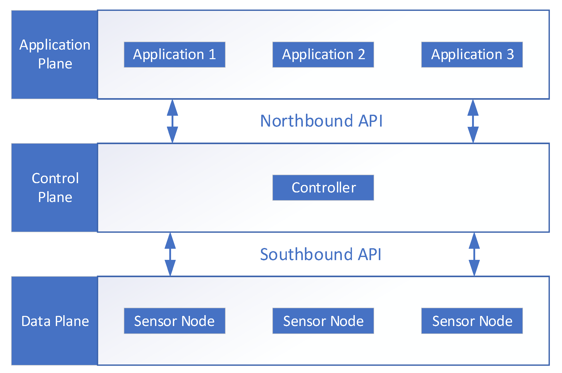
Figure 2.
Figure 2. Overview of the ATAW-TM.
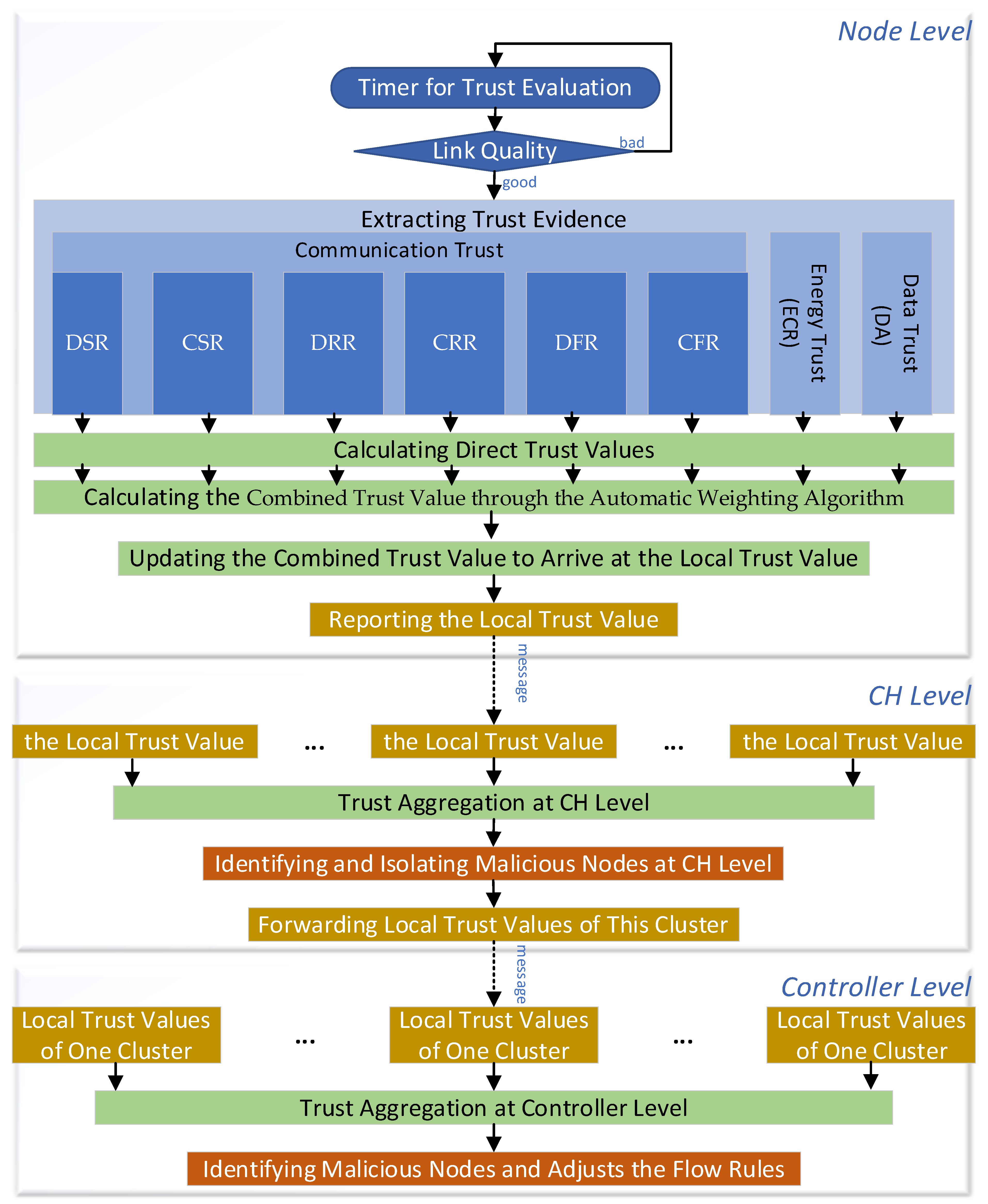
Figure 3.
Trust Evidence and the Corresponding Extraction Methods.
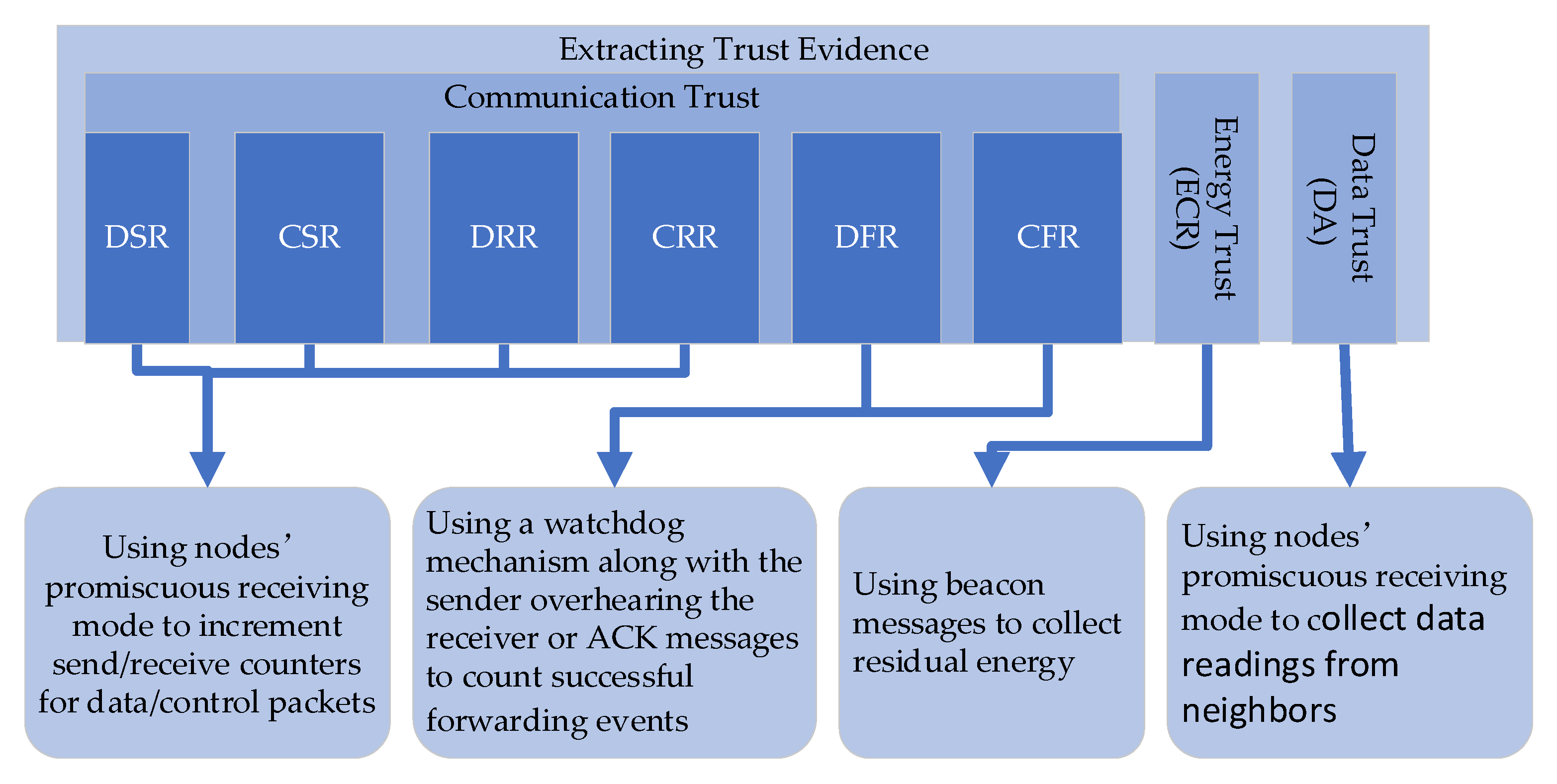
Figure 4.
The processes of direct trust value calculation.
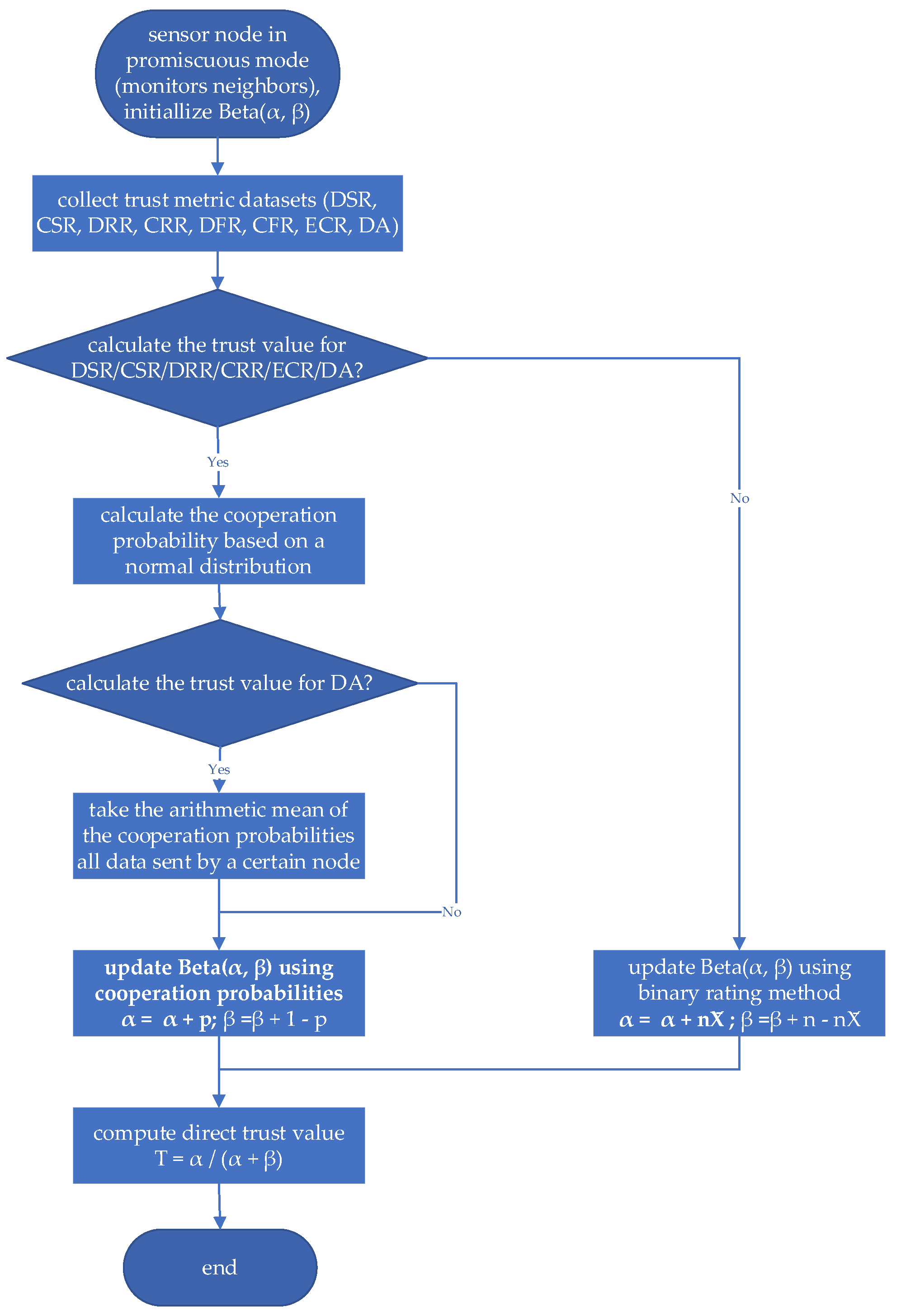
Figure 5.
Gaussian Distribution PDF Curve.
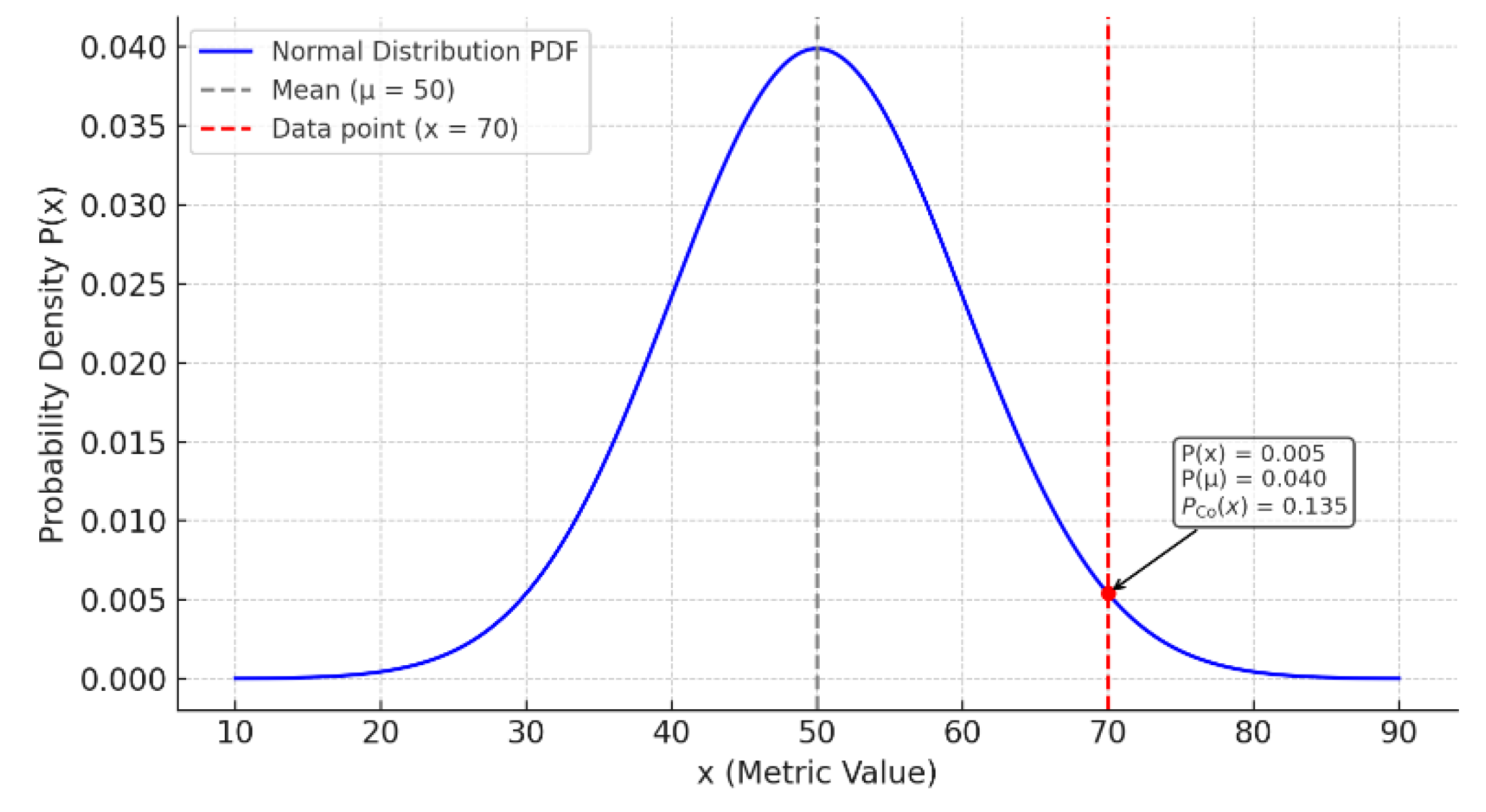
Figure 6.
Cooperation Probability Function Curve.
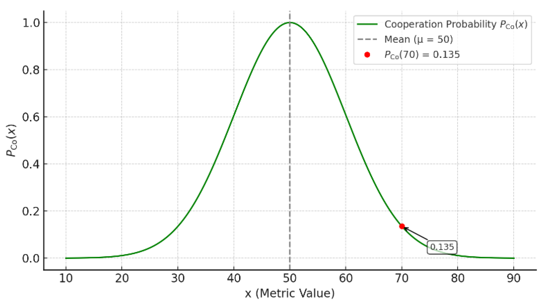
Figure 7.
The format of the SDN-WISE report message.
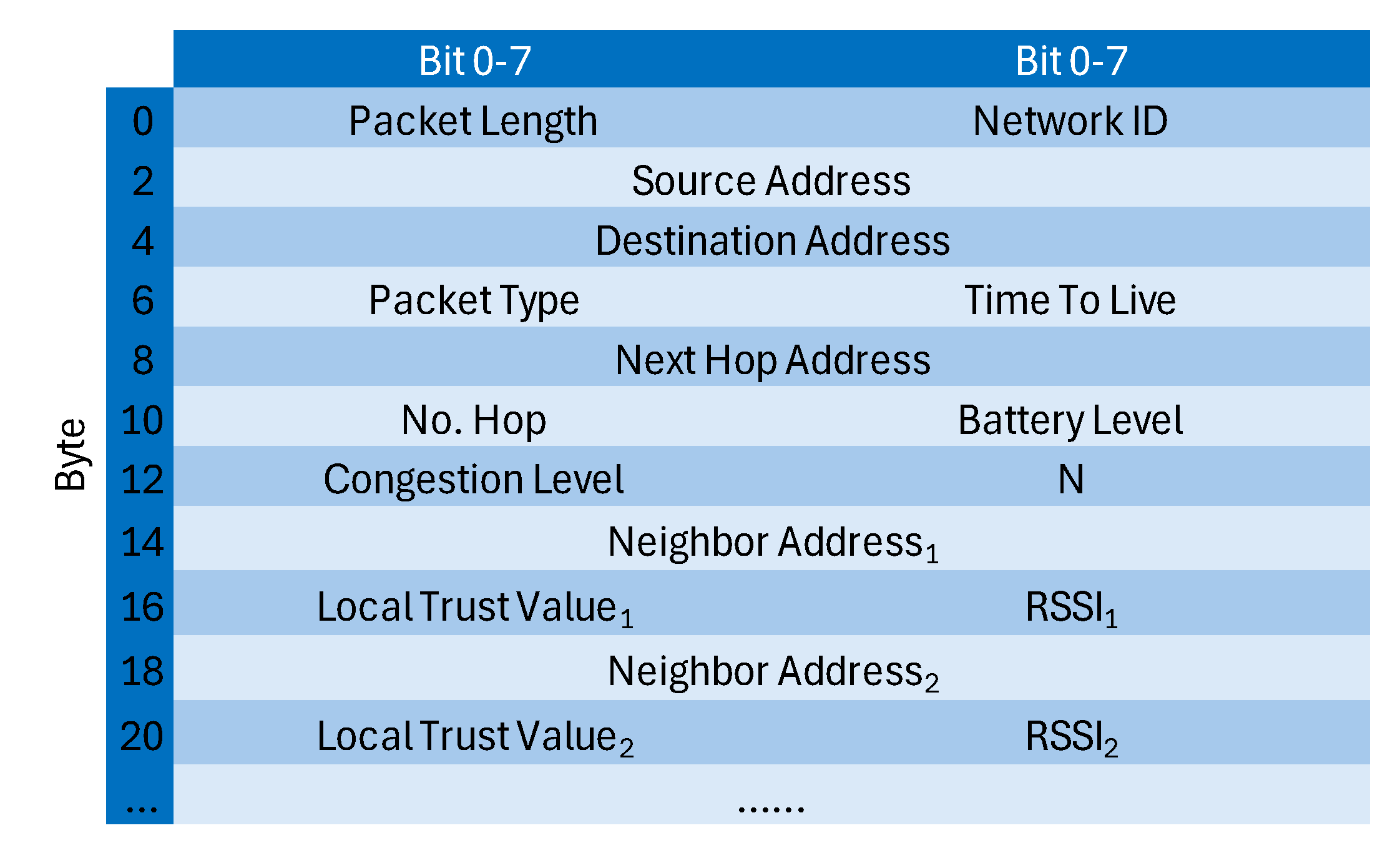
Figure 8.
An example of a flow table in SDN-WISE.
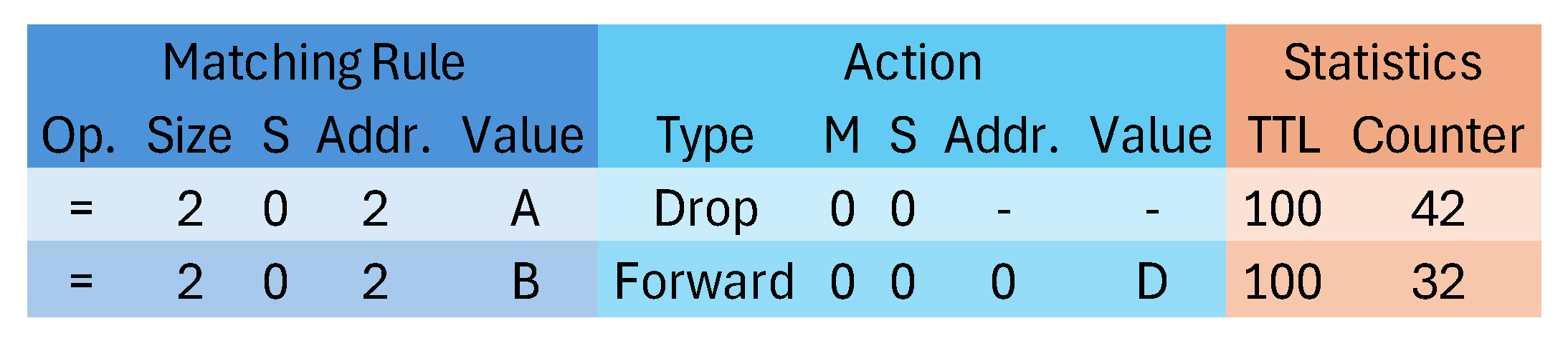
Figure 9.
The format of the trust information request/reply message.
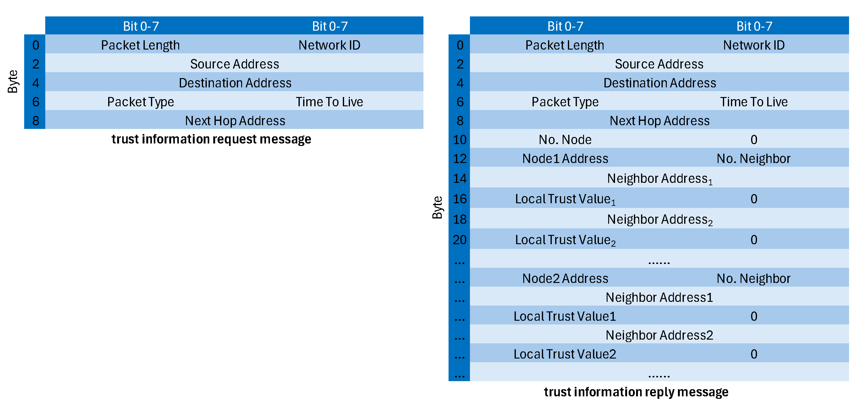
Figure 10.
Data Packet Sending Count vs Direct Trust Value in Scenario 1.
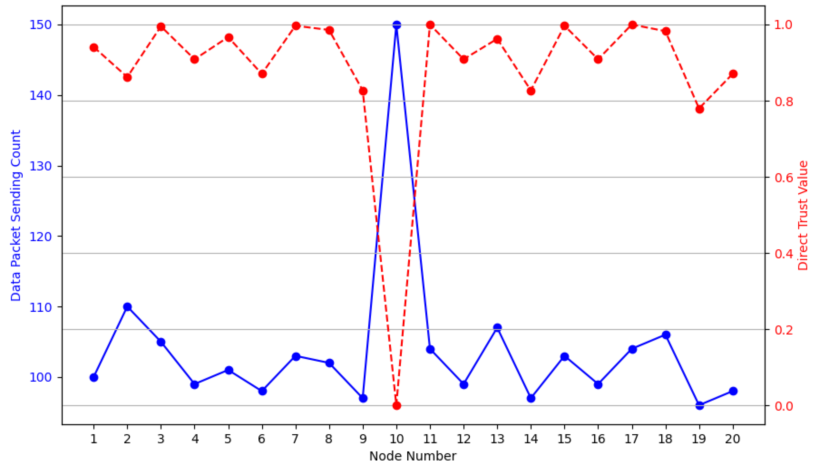
Figure 11.
Data Packet Sending Count vs Direct Trust Value in Scenario 2.
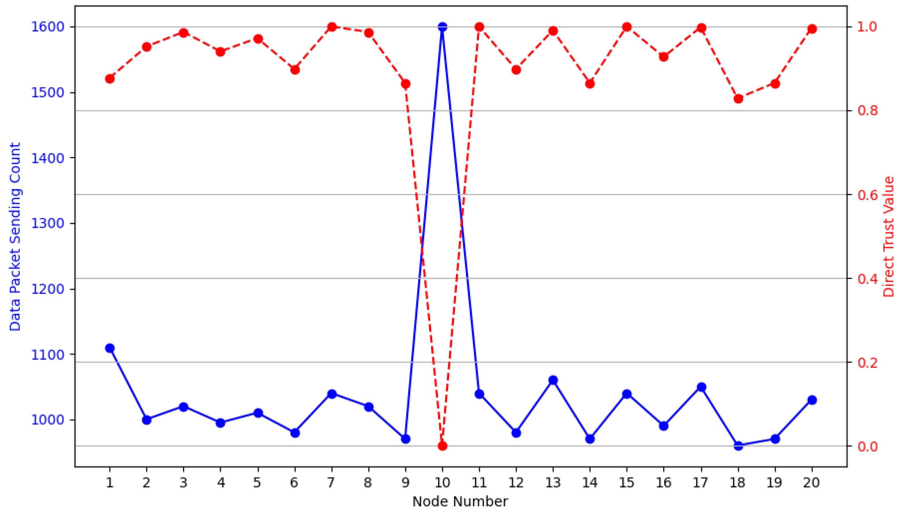
Figure 12.
Direct Trust Value and Weight Comparison.
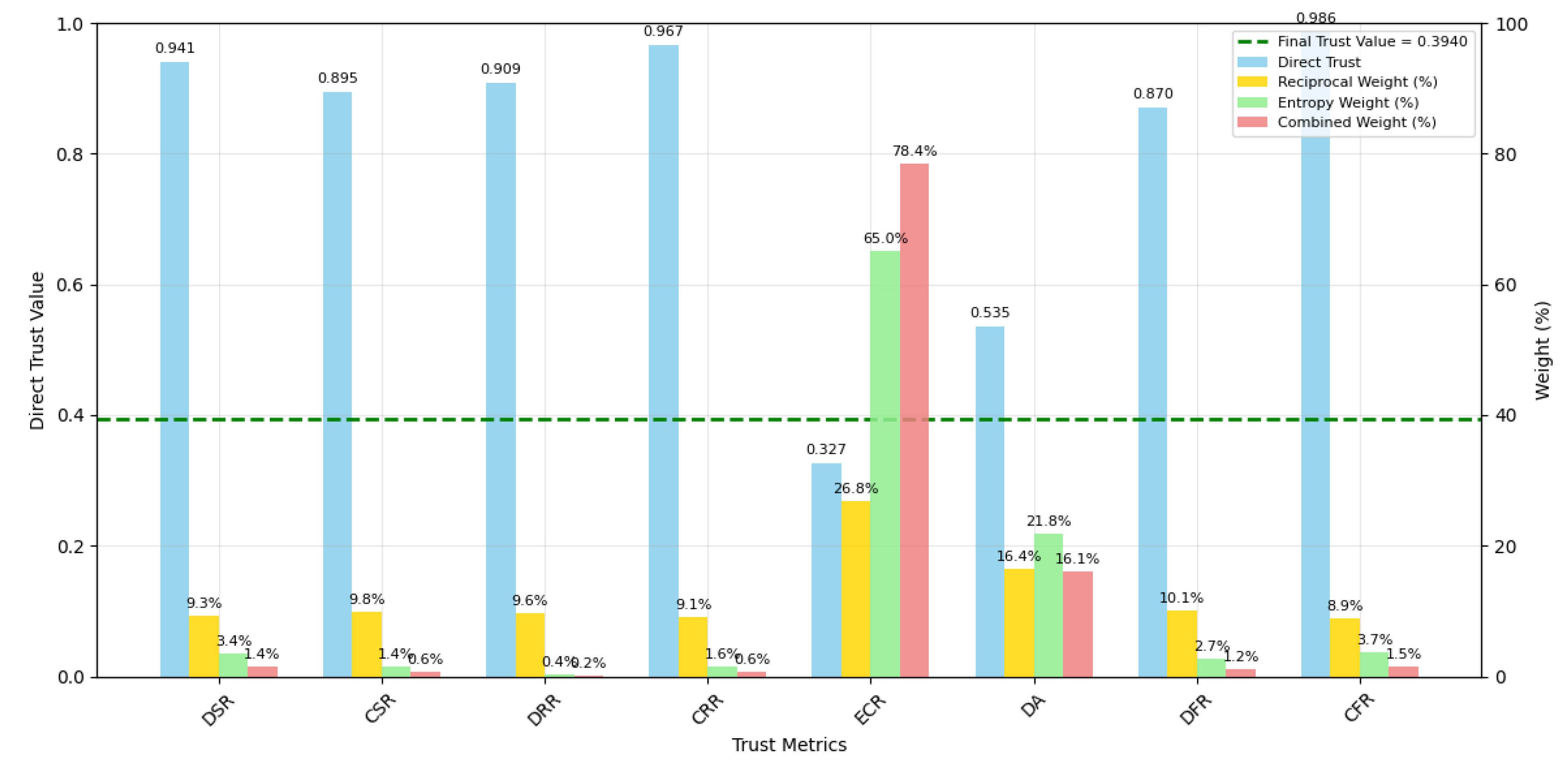
Figure 13.
the Trust Change vs the Aging Factor.
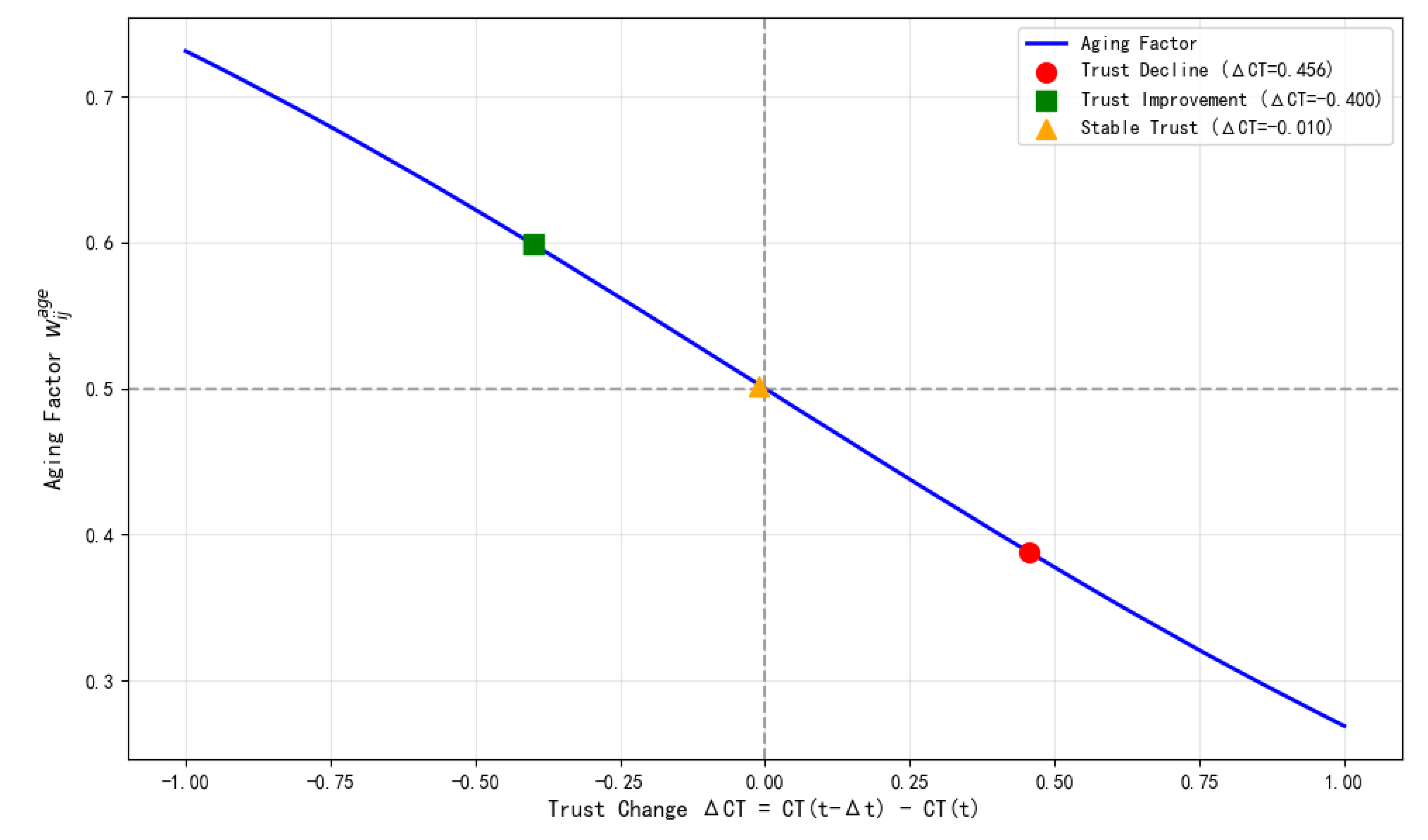

Table 1.
Dataset for each metric.
| ) | Description of Data Collection | |
|---|---|---|
| DSR | . | |
| CSR | . | |
| DRR | . | |
| CRR | . | |
| ECR | , calculated as the starting energy (from previous beacons) minus the remaining energy (from beacons at the end of the period). | |
| DA | , and may vary across different nodes. |
Table 2.
The relationship between these parameters for all six metrics.
| Metric | ) | ) | ) | ) |
|---|---|---|---|---|
| DSR | ||||
| CSR | ||||
| DRR | ||||
| CRR | ||||
| ECR | ||||
| DA |
Table 3.
Entropy values computed with different bases.
| Bases | Entropy values |
|---|---|
| 2 | |
| e | |
| 10 |
Table 4.
Entropy values of different probability distribution computed with different bases.
| Probability . | |||
|---|---|---|---|
| (0.8, 0.2) | 0.7219 | 0.5004 | 0.2173 |
| (0.6, 0.4) | 0.9710 | 0.6730 | 0.2923 |
| (0.5, 0.5) | 1.0000 | 0.6931 | 0.3010 |
Table 5.
Direct trust values for each node.
| Node | Data Packet Sending Count | Direct Trust Value |
|---|---|---|
| Node 1 | 100 | 0.941106 |
| Node 2 | 110 | 0.862004 |
| Node 3 | 105 | 0.995183 |
| Node 4 | 99 | 0.908630 |
| Node 5 | 101 | 0.966995 |
| Node 6 | 98 | 0.870300 |
| Node 7 | 103 | 0.996773 |
| Node 8 | 102 | 0.985697 |
| Node 9 | 97 | 0.826960 |
| Node 10 | 150 | 0.000207 |
| Node 11 | 104 | 0.999960 |
| Node 12 | 99 | 0.908630 |
| Node 13 | 107 | 0.962375 |
| Node 14 | 97 | 0.826960 |
| Node 15 | 103 | 0.996773 |
| Node 16 | 99 | 0.908630 |
| Node 17 | 104 | 0.999960 |
| Node 18 | 106 | 0.982555 |
| Node 19 | 96 | 0.779532 |
| Node 20 | 98 | 0.870300 |
Table 6.
Weighting Analysis Results.
| Trust Metric | Direct Trust Value | Reciprocal Weight | Entropy Weight | Combined Weight | Weighted Trust Value |
|---|---|---|---|---|---|
| DSR | 0.9411 | 1.062 | 0.034 | 0.014 | 0.0136 |
| CSR | 0.8952 | 1.117 | 0.014 | 0.006 | 0.0056 |
| DRR | 0.9086 | 1.100 | 0.004 | 0.002 | 0.0014 |
| CRR | 0.9670 | 1.034 | 0.016 | 0.006 | 0.0062 |
| ECR | 0.3269 | 3.058 | 0.650 | 0.784 | 0.2563 |
| DA | 0.5350 | 1.869 | 0.218 | 0.161 | 0.0860 |
| DFR | 0.8703 | 1.149 | 0.027 | 0.012 | 0.0105 |
| CFR | 0.9857 | 1.014 | 0.037 | 0.015 | 0.0144 |
| Combined Trust Value 0.3940 | |||||
Table 7.
Weighting Analysis Results.
| Scenario | CT(t-Δt) | CT(t) | ΔCT | Aging Factor | Local Trust |
|---|---|---|---|---|---|
| Trust Decline | 0.850 | 0.394 | 0.456 | 0.388 | 0.571 |
| (additional) Trust Improvement | 0.400 | 0.800 | -0.400 | 0.599 | 0.561 |
| (additional) Stable Trust | 0.700 | 0.710 | -0.010 | 0.502 | 0.705 |
Disclaimer/Publisher’s Note: The statements, opinions and data contained in all publications are solely those of the individual author(s) and contributor(s) and not of MDPI and/or the editor(s). MDPI and/or the editor(s) disclaim responsibility for any injury to people or property resulting from any ideas, methods, instructions or products referred to in the content. |
© 2025 by the authors. Licensee MDPI, Basel, Switzerland. This article is an open access article distributed under the terms and conditions of the Creative Commons Attribution (CC BY) license (http://creativecommons.org/licenses/by/4.0/).
Copyright: This open access article is published under a Creative Commons CC BY 4.0 license, which permit the free download, distribution, and reuse, provided that the author and preprint are cited in any reuse.


