
Submitted:
16 November 2025
Posted:
17 November 2025
You are already at the latest version
Abstract
Zonal day-ahead (DA) electricity markets followed by redispatch (RD) markets for congestion management are vulnerable to the strategic bidding behavior known as Inc-Dec gaming. Although previous literature has demonstrated the effects of Inc-Dec gaming, it has neglected the participation of flexible demand in RD markets. This paper addresses this gap by developing a novel multi-period bi-level optimization model of a strategic producer participating in DA and RD markets, accounting for the inherent time-coupling operating characteristics of demand flexibility (DF) in the RD market. This model includes an upper level problem determining the optimal bidding decisions of the strategic producer in the DA and RD markets, and two lower level problems representing the clearing process of the two markets. The impacts of DF in mitigating Inc-Dec gaming are demonstrated through a small-scale case study involving a 2-node system and a 2-period market horizon, as well as a large-scale case study involving a modified IEEE RTS 24-node system and a daily (24-hour) market horizon.
Keywords:
bi-level optimization
; demand flexibility
; electricity markets
; Inc-Dec gaming
; redispatch markets
1. Introduction
1.1. Background and Motivation
Deregulated and highly renewable energy systems are characterized by more variable and less predictable power flows within the transmission network [1]. In this context, Transmission System Operators (TSOs) carry out the critical task of managing grid congestion. In the US, this is primarily addressed through the application of nodal pricing, which accounts for transmission constraints and varying costs of delivering electricity at different nodes across the network. In contrast, the EU target model relies on a zonal day-ahead (DA) market, followed by redispatch (RD) markets as the main ex-post remedial action used by TSOs to adjust DA schedules, resolve grid congestion, and maintain grid stability [2].
In 2023, Germany, Poland, and Spain each carried out RD activations corresponding to approximately 5% of their total electricity demand - a record level - in order to resolve transmission grid congestion. According to data from the EU Agency for the Cooperation of Energy Regulators (ACER), this costed £2 billion in Germany alone [3]. While this trend is in part driven by the ongoing large-scale integration of non-dispatchable renewable energy, in recent years, the European Commission has also highlighted [4] that the RD process is vulnerable to the strategic bidding behaviour called Inc-Dec (or Incremental-Decremental) gaming - which could contribute to the observed rise in RD volume and cost.
Within the electricity markets literature, the terms strategic bidding and market power generally refer to a producer’s ability to influence market prices (through economic withholding or capacity withholding) within a single market stage [5]. In [6] the concept of locational market power is discussed, which may arise even in the absence of congestion, as strategic producers can induce binding network constraints through their bids. The Inc-Dec game represents a (still largely unexplored) extension of this concept to a market framework with sequential stages, where producers exploit the interaction between DA and RD markets rather than a single-stage price effect. Through Inc-Dec gaming, producers can exploit the DA market to induce artificial scarcity or surplus in their node, to influence the subsequent RD market, ultimately increasing their profit [7]. Inc-Dec gaming played a crucial role in the U.S. transition to nodal pricing [8] and has been empirically evidenced in the U.K. [9], Italy [10], and Germany [11]. This mechanism therefore links strategic DA behaviour to redispatch outcomes rather than to single-market price manipulation, making it a distinct, inter-temporal manifestation of market power.
To address these concerns, several scholars have examined the issue, mainly through game theoretical analysis of simplified representations of the European network and markets’ rules. The early contribution in [12] analytically derives the Nash equilibrium for a continuum of infinitesimally small producers under various market design scenarios. It demonstrates that a zonal DA market, followed by a pay-as-bid RD market, results in additional payments to producers in export-constrained nodes due to Inc-Dec gaming, thereby leading to inefficient investment signals. These results are confirmed in [13], which considers pay-as-clear pricing in the RD market, and [14], which also considers demand-driven uncertainty on network congestion. However, both analyses are limited to a 2-node system. Reference [15] introduces an Equilibrium Problem with Equilibrium Constraints (EPEC) model that is reformulated as a Mixed-Integer Linear Programming (MILP) model, enabling the study of larger networks. In [16], this approach is applied to investigate the impact of Inc-Dec gaming under two different RD pricing options: pay-as-bid and optimal zonal pricing, the latter proposed by the authors. By focusing on surplus nodes in a 6-node and a 24-node system, the analysis demonstrates that RD with pay-as-bid pricing is less efficient than optimal zonal pricing, where the geographical price granularity in RD matches that of the DA market (i.e., zonal). Rather than focusing on market equilibrium calculations, reference [17] introduces a bi-level model for the strategic bidding of a single producer. Authors consider grid congestion at both the distribution and transmission levels, carrying out analysis on a meshed 3-node transmission network linked to two branches of a radial distribution network.
Beyond the above challenges associated with managing transmission congestion, another fundamental feature of the emerging energy systems is the enhanced role of the demand side, whose flexibility (i.e., the ability of modifying its temporal patterns) is widely considered as a key enabler towards achieving cost-efficient decarbonization [18]. Currently, consumers are legally eligible to participate in RD markets in Austria, Finland, France, the Netherlands, Norway, Romania, and Sweden [19]. At the same time, TSOs can also access innovative platforms such as GOPACS [20] and NODES [21] to procure congestion management services.
Therefore, a relevant research gap emerges in this context: previous literature on Inc-Dec gaming (as summarized in Table 1) has focused on generation-only RD markets, neglecting demand-side participation. Going further, existing studies have merely focused on single-period models, thus being inherently unable to capture the time-coupled operating characteristics of demand flexibility (DF).
1.2. Scope and Contribution
As indicated in Table 1, this paper aims to fill this knowledge gap by investigating for the first time the participation of DF in RD markets, while accounting for its time-coupling operating characteristics, and analyzing the impacts of such participation on Inc-Dec gaming. Specifically, the novel contributions of this paper are as follows:
- A multi-period bi-level optimization model of a strategic producer participating in DA and RD markets is proposed, accounting for network constraints and the time-coupling operating characteristics of DF participating in the RD market. The upper level problem determines the optimal bidding decisions of the strategic producer in the DA and RD markets, while the two lower level problems represent the clearing process of the two markets. This bi-level problem is solved by converting it into a Mathematical Program with Equilibrium Constraints (MPEC) and subsequently to a MILP through strong duality and binary expansion techniques.
- The role of DF in addressing Inc–Dec gaming, as well as the generic applicability of the proposed model, are demonstrated through two case studies: a simple 2-node, 2-period example, and a large-scale case study based on a modified IEEE RTS 24-node system over a 24-hour horizon.
1.3. Paper Structure
The rest of this paper is organized as follows. Section 2 details the developed bi-level optimization model. The application of the model to an illustrative small-scale case study and a large-scale case study is presented in Section 3 and Section 4, respectively. Finally, Section 5 discusses conclusions and future extensions of this work.
2. Modeling Approach
2.1. Modeling Assumptions
The proposed bi-level optimization model expresses the perspective of a strategic conventional producer i who aims at optimizing its bidding decisions in order to maximize its total profit in the DA energy and RD markets, while anticipating the clearing outcomes of the two markets and potential DF activations in the RD market. For clarity reasons, the main assumptions behind this model are outlined below:
- The modeled DA market is a pool-based, energy-only, zonal market, cleared by the market clearing agent through the solution of a social welfare maximization problem which ignores within-zone network constraints and adopts pay-as-clear pricing.
- The modeled RD market is a pool-based, pay-as-bid (as commonly implemented in the EU) market, cleared by the TSO, who also acts as the sole buyer, in order to resolve within-zone network congestion with the minimum RD cost. The TSO employs a DC power flow model and Generation Shift Factors (GSFs) to represent network constraints. The RD market clearing follows the DA market clearing.
- Considering the focus of the paper, and for the sake of simplicity, the model considers a single bidding zone (the one where the strategic producer is located), and thus disregards market coupling.
- For clarity, and without loss of generality, the model assumes that each producer owns a single generation unit and submits a single price-quantity bid for this generation unit for each time period t and in each of the two considered markets. For the same reasons, the model assumes that each demand participant submits a single bid for each time period t, including in the RD market when the unit provides flexibility.
- Expanding the approach employed in [22], the strategic behavior of producer i is expressed through the decision variables , and . Specifically, expresses its behavior in the DA market with implying that it behaves competitively and reveals its actual marginal cost to the DA market, while and imply that it behaves strategically (overbids and underbids, respectively). In a similar fashion, and express its behavior in the RD market (upward and downward, respectively), with and implying that it behaves competitively.
- DF is incorporated in the RD market clearing problem through a generic, technology-agnostic, and inter-temporal model, which follows the approach of [23,24,25,26,27]. Specifically, the load of the demand participant j at time period t can be reduced or increased relative to its dispatch in the DA market, but a) this reduction/increase is subject to certain limits (prescribed by the relative parameter ), b) it entails a quantifiable marginal cost of discomfort [26] which also constitutes the price offered by j in the RD market (i.e., strategic behavior of flexible demand participants is neglected), and c) the total size of demand reductions is equal to the total size of demand increases within the considered daily market horizon, implying that demand shifting is energy neutral.
2.2. Bi-Level Optimization Model of Strategic Producer
The structure of the proposed bi-level optimization problem is illustrated in Figure 1 and involves three interdependent optimization problems; specifically, the upper level (UL) problem determines the optimal bidding decisions of the strategic producer i in the DA and RD markets, and is subject to two lower level problems, which represent the clearing process of the DA market (LL1) and the RD market (LL2). The detailed formulation of the bi-level problem is presented below:
(UL problem)
where:
(LL1 problem)
where:
subject to:
(LL2 problem)
where:
subject to:
The objective function of the UL problem (1) lies in maximizing the total profit of the strategic producer i in the DA and RD markets, which is determined as the difference between its revenues from the two markets and its operating cost and rearranging some terms. This objective is pursued by optimizing the strategic bidding variables (2).
The objective function of the LL1 problem (3) lies in minimizing the perceived negative social welfare of the DA market, by optimizing the market clearing decisions (4). This problem is subject to the demand-supply balance constraints for the considered (single) bidding zone (5) - whose associated dual variables constitute the DA market clearing prices - and the minimum and maximum dispatch limits of the market participants (6)-(9).
The objective function of the LL2 problem (10), lies in minimizing the perceived total RD cost incurred by the TSO - including both upward and downward adjustments - by optimizing the RD market clearing decisions (11). This cost includes RD actions on both the generation side, captured by the first two rows of (10), and the demand side, represented by the last row of the same equation. On the demand side, we consider upward and downward RD offers from participants with DF, as well as the cost of involuntary load curtailment actions, which are priced at the Value of Lost Load (VoLL). Constraints (12) ensure that the demand-supply balance for the considered bidding zone is preserved after the RD market clearing. Constraints (13) ensure that network congestion within the examined zone is resolved by the RD market i.e., the power flow on each line is lower or equal to its transmission capacity, employing a DC power flow model similar to [28], and GSFs. Constraints (14)-(19) express the minimum and maximum RD limits of the producers.
The DF of demand participant j in the RD market is expressed by constraints (20)-(22), following Assumption 6) of Section 2.1. Constraint (20) ensures that demand shifting is energy neutral within the examined daily horizon. Constraints (21) and (22) express the limits of demand reduction and increase, respectively, as a ratio of the dispatch in the DA market, reduced by any required involuntary load curtailment; implies that participant j does not exhibit any DF while implies that its whole energy consumption can be shifted in time. Finally, constraints (23) express the bounds of involuntary load curtailments.
2.3. MPEC Model of the Strategic Producer
As a first step towards solving the above bi-level optimization problem, LL1 and LL2 problems are replaced by their Karush–Kuhn–Tucker (KKT) conditions and the bi-level problem is converted to a single level MPEC, which is formulated as follows:
where:
subject to:
LL1 original equality condition: (5)
LL1 KKT optimality conditions:
LL1 compementarity constraints:
LL2 original equality conditions: (12), (20)
LL2 stationarity conditions:
LL2 complementarity constraints:
The MPEC shares the same objective function as the UL problem. The set of decision variables (25) includes the decision variables of the UL, LL1, and LL2, along with the dual variables (26) associated with the constraints of LL1 and LL2. The KKT optimality conditions are expressed by (27)-(38) and (39)-(67), for LL1 and LL2, respectively.
2.4. MILP Model of the Strategic Producer
Since the above MPEC model is non-linear, we convert it to a MILP model which can be effectively solved through commercial solvers. Specifically, the MPEC model includes three different categories of non-linearities which we address through suitable linearization techniques. The first one involves the bi-linear term in the objective function (24). This term is linearized by applying the strong duality theorem to LL1 and exploiting the KKT conditions (31) and (32), as follows (full derivation provided in Appendix A of the supplementary document [29]):
The second non-linearity involves the bi-linear terms and in the objective function (24). These terms are linearized through binary expansion [30]. This technique requires introducing the auxiliary variables:
where and are binary variables and and are linear dummy variables. Let and be two sets of B discrete values in the range and , respectively. Then, the variables and can be replaced with the following sums of binary variables:
where and . Multiplying both sides of (70) and (71) by and , respectively, summing for every t, and defining the new dummy variables and , results in:
Therefore, the bilinear terms and can be replaced by their discrete approximation, on the right side of (72) and (73), respectively. The product of variables in (74) and (75) can be transformed into the following equivalent mixed-integer linear constraints:
where G is a positive constant that is large enough for the constraints (76) and (78) to be relaxed when and , and for the constraints (77) and (79) to be relaxed when and , respectively.
The third non-linearity involves the bi-linear terms in the complementarity conditions (31)-(38) and (48)-(67), which can be expressed in the general form , with and p representing generic dual and primal terms respectively. They are linearized using the Fortuny-Amat approach [31] (i.e. big-M). By introducing an auxiliary binary variable , each of these conditions is replaced with the set of mixed-integer linear expressions , , , where and M are large positive constants.
3. Small-Scale Case Study
This section presents a simple case study to illustrate the effects of DF in mitigating Inc-Dec gaming, considering the 2-node system illustrated in Figure 2 and a simplified market involving only 2 time periods (a peak period t = 1 and an off-peak period t = 2) for both DA and RD markets. In this case study, the strategic producer i (which employs the model of Section 2 to optimize its bidding decisions) is connected to the import-constrained node 2. This producer is assumed to have a lower marginal cost than the other competing producer , connected to node 1.
The parameters of the two producers and the single demand participant j are presented in Table 2 and Table 3. For the binary expansion of the linear variables and (Section 2.4), we employ , , and . In order to comprehensively assess the role of DF in addressing Inc-Dec gaming, we implement and compare three different scenarios:
- Benchmark: All producers behave competitively in both DA and RD markets, while the demand does not exhibit any DF. This scenario is implemented by forcing in the proposed model, as well as setting
- Strategic: The producer connected to node 2 behaves strategically in the DA and RD markets by employing the proposed model with , , being decision variables. The demand does not exhibit any DF ().
- Strategic + DF: The producer connected to node 2 behaves strategically in the DA and RD markets, and the demand exhibits DF characterized by .
In this study, the three modelled scenarios represent different stages in the evolution of the European RD market. The Benchmark scenario reflects a design with cost-based, ex-post remuneration mechanisms for RD. The Strategic scenario corresponds to the current configuration of early generation-only RD markets. Finally, the Strategic + DF scenario illustrates a more advanced market in which flexible demand participates on a level-playing field with generation in RD processes. Strategic behaviour may emerge in the latter two.
3.1. Increase-Decrease (Inc-Dec) Gaming
The effects of Inc-Dec gaming are demonstrated by comparing results from the scenario Strategic against those from the scenario Benchmark, thus neglecting for now DF. These results are presented in Table 4 and Table 5. In the Benchmark scenario, where both producers act competitively, producer i supplies the entire demand in each period of the DA market due to its lower marginal cost, while producer ’s offers are not accepted (Table 4). As a result, the network is not subject to any congestion, RD actions are unnecessary, and the daily system cost (£14,000) consists only of the DA market cost (Table 4). The producer connected to node 2 is the marginal producer and does not provide any RD power, therefore achieving a net daily profit of zero (Table 5).
In the scenario Strategic, where producer i bids strategically, an instance of Inc-Dec gaming emerges at the peak period . Specifically, the strategic producer overbids in the DA market (i.e., it offers a price higher than its marginal cost, as indicated by the strategic variable , in Table 5), thereby ensuring exclusion from the DA accepted offers (i.e. economic withholding). As a consequence, the whole demand at this period is covered by the competing producer connected to node 1 (Table 4) therefore creating congestion in line l to be resolved through RD actions. The strategic producer then exploits this situation by offering upward RD at the highest possible price (as indicated by the strategic variable , in Table 5).
Consequently, it earns a profit of £7,500 at (which is entirely achieved in the RD market) while its respective profit in the scenario Benchmark was zero. Note that the strategic producer also earns a positive profit at , but this is driven by mere overbidding in the DA market and not Inc-Dec gaming and thus is not discussed further. Overall, the daily system cost in this scenario is increased to £26,000, compared with £14,000 in the Benchmark scenario, with the largest part of this negative effect attributable to the Inc-Dec gaming instance at .
3.2. Role of DF in Addressing Inc-Dec Gaming
Similar to the scenario Strategic (discussed in Section 3.1), the strategic producer still engages in Inc-Dec gaming during the peak period () in the scenario Strategic + DF. However, the demand participant now contributes to the upward RD during this period by reducing its demand by MW (Table 4), which represents its maximum possible alteration from the DA clearing, under the DF constraints ()-(). Consequently, the strategic producer’s upward RD activation decreases from 500 MW to 420 MW (Table 4), which reduces its profit during this period from £7,500 to £6,300 (Table 5).
Nevertheless, due to the energy neutrality constraint of DF (20), the demand participant needs to increase its demand by MW at the off-peak period . Therefore, considering the RD balance constraint (12), the strategic producer exploits this situation by offering upward RD of the same amount (Table 4). However, note that this offer is not made at the highest possible price but at a lower one (as indicated by the strategic variable in Table 5), as a higher offer would render the strategic producer out of the RD merit order and the required upward RD would be provided by the competing producer (in the off-peak period the two nodes are not decoupled by network congestion). As a result, its profit at this period is increased from £2,000 to £2,400.
Considering both time periods, although DF does not affect the overall consumption (the demand reduction at is equal to the demand increase at ), it yields a positive impact in terms of mitigating Inc-Dec gaming, since the overall profit of the strategic producer is reduced from £9,500 to £8,700 (Table 5) as the profit reduction during the peak period outweighs the profit increase during the off-peak period. This positive impact is also reflected on the overall system cost, which is reduced from £26,000 to £25,280 (Table 4).
4. Large-Scale Case Study
This section aims at demonstrating the applicability of the proposed model and the role of DF in addressing Inc-Dec gaming through a large-scale and more realistic case study. We consider a 24-hour market horizon and the modified IEEE RTS 24-node system illustrated in Figure 3. The various parameters of the network (including reactance and capacity of each line), conventional producers (including the marginal cost and maximum power output of each producer), wind producers (including the profile and distribution by node), and the demand units (including the maximum baseline profile and demand distribution by node), are based on [32,33,34] and provided in Appendix B.
As in the small-scale case study (Section 3), three similar scenarios (Benchmark, Strategic, Strategic + DF) are compared. In the latter two scenarios, we assume that producer connected to node 18 (highlighted in yellow in Figure 3) acts as a strategic producer. This producer has the highest marginal cost among all producers (Table A4), in contrast to the small-scale case study where the strategic producer had the lowest marginal cost. This choice is made intentionally to demonstrate that Inc-Dec gaming is relevant to producers with different positions in the merit order. In addition, to evaluate how DF affects the economics of the RD market in the presence of Inc-Dec gaming, in the scenario Strategic + DF, demand participants connected to node 10, 13, and 15 (indicated in green in Figure 3) exhibit DF characterized by . The upward and downward discomfort costs for DF range from 0 £/MW to 1 £/MW within the day, and follow the rationale of [27]. Specifically, shifting demand away from a period incurs a discomfort cost proportional to the inverse of that period’s baseline demand, whereas shifting demand toward a period incurs a cost proportional to the baseline itself. The wind producers k are assumed to have a marginal cost of zero. The lines connecting node pairs (14,16) and (15,21) constitute critical network elements, as they are congested during certain hours even under perfect competition assumptions (i.e. in the Benchmark scenario).
These lines are shown in red in Figure 3, with arrows indicating the direction of power flow during hours with grid congestion. Specifically, congestion on these lines is caused by power flows from the north-western (nodes 16-18 and 21-22) to the southern part of the system, since 74% of the system demand is located south of the critical network elements (nodes 1-15 and 24), where only 37% of the installed generation capacity is located.
Considering the most generic scenario Strategic + DF, the proposed MILP model (Section 2.4) has 11,033 continuous variables, 7,968 binary variables, and 18,569 constraints. This model has been implemented using the GUROBI Python Interface [35] and solved through the Gurobi Optimizer solver on a computer with a 28-core 2.6 GHz Intel Xeon processor and 512 GB of RAM. This scenario has been solved in 1,931 seconds with the mixed-integer programming gap set to 1%.
4.1. Increase-Decrease (Inc-Dec) Gaming
As in the small-scale case study presented in Section 3, the effects of Inc-Dec gaming are demonstrated by comparing the scenario Strategic against the scenario Benchmark. In the latter, the offers of the examined producer 9 are not accepted in either the DA or RD market throughout the day, as it exhibits the highest marginal cost. Consequently, it achieves a daily profit of zero (Table 7).
In the scenario Strategic, Inc-Dec gaming emerges during hours 07:00-23:00.
Specifically, the strategic producer underbids in the DA market (i.e., it offers a price lower than its marginal cost, as indicated by the strategic variables in Table 6) in order to ensure its offers are accepted in the DA clearing. Figure 4 shows the DA clearing by producers’ category, i.e. wind producers k, strategic producer , and all other conventional producers . As a consequence, during these hours, the DA dispatch of conventional producers at nodes 2, 7, 15, 16, and 23 is replaced by dispatch of strategic producer , and the overall extent of congestion is increased by 107% with respect to the Benchmark scenario (Table 7).
Specifically, as illustrated in Figure 5, the strategic action of producer exacerbates congestion on lines (14,16) and (15,21), while also inducing additional congestion on lines (16,17) and (13,23). The strategic producer then exploits this situation by offering downward RD at an average price of 7.69 £/MWh (as indicated by the average value of 0.29, Table 6). As a result, producer is redispatched downwards in hours 07:00-23:00, as illustrated in Table 6 and in the left chart of Figure 6. Although it incurs losses in the DA market (due to underbidding), its total daily profit increases from zero (Benchmark scenario) to £39,108. This instance of Inc-Dec gaming increases the daily RD cost from £39,284 to £81,228 (Table 7).
4.2. Role of DF in Addressing Inc-Dec Gaming
In the scenario Strategic + DF the DA market clearing does not change with respect to the scenario Strategic (Figure 4 and left side of Table 7). However, for what concerns the RD market, results in , together with Figure 6, indicate two important effects of DF.
With respect to system costs, the introduction of DF lowers RD costs by 8% (from £81,228 to £74,981, Table 7) over the 24-hour period. The right chart of Figure 6 shows that in peak hours 10:00-20:00 the flexible demand units are activated upwards (i.e. demand is reduced). This yields two economic advantages: (i) it reduces upward RD reliance on peaking producer (whose marginal cost is 20.93 £/MWh). This producer is slightly more expensive than the other producer providing upward RD in those hours (), and considerably more expensive than DF, thereby lowering the effective cost of upward RD. (ii) In most of the hours (e.g., 13:00), it also reduces the total volume of RD required. The latter is due to the higher congestion-relief effectiveness of DF, as part of it is located at node 15, which is directly connected to a congested line and thus associated with a high GSF.
In off-peak and shoulder hours 00:00-06:00 and 21:00-23:00, owing to the energy-neutrality constraint (20), DF is activated downwards (i.e., demand increases). This additional consumption is supplied primarily by low-cost conventional producers (, with marginal costs between 0.50 £/MWh and 13.32 £/MWh) and wind producers () that bid at zero, allowing DF to absorb low-priced energy. Notably, the upward RD of wind producers in hours 04:00–05:00 illustrates DF’s ability to reduce day-ahead wind curtailment (Figure 6).
Therefore, as in the small-scale case study, the RD cost reduction driven by DF during peak hours outweighs the RD cost increase during off-peak hours, resulting in an overall positive effect of DF in terms of system costs.
With respect to the profit of the strategic producer, a counter intuitive result emerges: although DF reduces the total RD cost of the system, the profit of the strategic producer in the RD market increases. This is because, thanks to the two system-level economic benefits explained above, the cost per MW of congestion relief decreases in the Strategic + DF scenario. This enables the strategic producer to slightly adjust its offers in a more convenient way while still remaining selected in the TSO’s optimal RD bundle solution. For example, in hours 15:00 and 19:00, the downward strategic variable is reduced from 0.32 to 0.25 (Table 7). By lowering , producer captures a higher profit , under pay-as-bid downward RD. In particular, its profit increases by approximately 4%, from £39,108 to £40,834, when DF participates in the RD market in this case study (Table 6).
5. Conclusion and Future Work
Despite increasing attention on the rising costs of redispatch in the European electricity markets and the impact of Inc-Dec gaming, existing literature solely focuses on market models with single time period analyses and is therefore unable to consider demand-side redispatch. As a result, those models fail to fully capture the redispatch markets economics, particularly the role of demand-side integration and the costs associated with Inc-Dec strategies.
This paper introduces a novel optimization model that extends existing Inc-Dec gaming models across multiple time periods and integrates technology-agnostic demand flexibility characteristics into a bi-level market modeling structure. The model features two lower-level problems representing the day-ahead and redispatch markets clearing and employs binary expansion techniques to linearize equations relating to pay-as-bid redispatch decisions. The resulting MILP formulation is tractable using commercial solvers and the proposed approach is demonstrated through two case studies.
These case studies show that Inc-Dec gaming emerges as the optimal strategy for producers located in import-constrained nodes of a small network (Section 3), as well as producers in a larger network with critical network elements (Section 4). In both situations, the activity of the strategic producer worsens grid congestion; a situation that the producer exploits to increase its profit, thereby distorting market outcomes. The large-scale case study also demonstrates that possessing market power in the day-ahead market is not a prerequisite for engaging in Inc–Dec gaming, as profit opportunities can arise purely from the locational and temporal structure of redispatch price signals.
From the system perspective, the introduction of demand flexibility in the redispatch stage, decreases total redispatch costs (around 8% in the case study of Section 4). This goes hand in hand with a reduction of Inc–Dec gaming in the case study of Section 3. Conversely, in the large-scale case (Section 4), a small exploitable bidding slack persists, enabling a marginal increase in strategic profit despite an unchanged congestion pattern.
These model-based findings depend on the specific market design assumptions and parameter settings adopted. Future research should aim to extend the model by incorporating demand flexibility also in the day-ahead timeframe, examining interactions among multiple strategic producers, and exploring the effects of uncertainty in demand and renewable generation.
Author Contributions
Conceptualization, formal analysis, investigation, data curation, writing—original draft preparation, L.P.; methodology, validation, L.P. and D.P.; software, L.P. and D.Q.; writing—review and editing, L.P., D.P., V.T.; supervision, D.P. and G.S.; project administration, G.S. All authors have read and agreed to the published version of the manuscript.
Funding
This research received no external funding.
Conflicts of Interest
The authors declare no conflicts of interest.
Nomenclature
| Indices and Sets | |
| Index and set of time periods | |
| i | Index of strategic conventional producer |
| Index and set of conventional producers other than i | |
| Index and set of renewable producers | |
| Index and set of demands | |
| Index and set of network nodes | |
| Index and set of network lines | |
| Subset of conventional producers i connected to n | |
| Subset of conventional producers other than i connected to n | |
| Subset of renewable producers k connected to n | |
| Subset of demands j connected to n | |
| Parameters | |
| Marginal benefit of demand j [£/MWh] | |
| Discomfort cost of demand j for shifting demand away from t [£/MWh] | |
| Discomfort cost of demand j for shifting demand towards t [£/MWh] | |
| VoLL | Value of lost load [£/MWh] |
| Maximum power of conventional producer i [MW] | |
| Maximum power of renewable producer k at t [MW] | |
| Maximum baseline power of demand j at t [MW] | |
| Generation Shift Factor between node n and line l | |
| Transmission capacity of network line l [MW] | |
| Load shifting limit of demand j [%] | |
| Variables | |
| Day-ahead market dispatch of producer i at t [MW] | |
| Day-ahead market dispatch of demand j at t [MW] | |
| Day-ahead market clearing price at t [£/MWh] | |
| Day-ahead strategic bidding variable of producer i at t | |
| Upward redispatch strategic bidding variable of producer i at t | |
| Downward redispatch strategic bidding variable of producer i at t | |
| Upward redispatch provided by producer i at t [MW] | |
| Downward redispatch provided by producer i at t [MW] | |
| Power of demand j shifted away from t [MW] | |
| Power of demand j shifted towards t [MW] | |
| Unserved power of demand j at t [MW] |
Abbreviations
The following abbreviations are used in this manuscript:
| ACER | EU Agency for the Cooperation of Energy Regulators |
| DA | Day-ahead |
| DF | Demand flexibility |
| EPEC | Equilibrium Problem with Equilibrium Constraints |
| GSF | Generation Shift Factor |
| KKT | Karush–Kuhn–Tucker |
| LL | Lower Level |
| MILP | Mixed-Integer Linear Programming |
| MPEC | Mathematical Program with Equilibrium Constraints |
| TSO | Transmission System Operator |
| RD | Redispatch |
| UL | Upper Level |
Appendix A. Strong Duality Applied to Day-Ahead Revenues
The bi-linear term in (24) representing revenues from the day-ahead market is . This term can be linearised by adopting linearization techniques exploiting the strong duality theorem [36] of LL1. As a first step, by multiplying both sides of (27) by , summing all terms over t, and applying the constraints in (31) and (32) the following expression is obtained:
Applying the strong duality theorem to LL1 we have that:
and therefore can be expressed in the exact linear form:
Appendix B. Data Input IEEE 24-Nodes Case Study
The IEEE 24-bus RTS system (Figure 3), widely recognized for evaluating power system reliability and market performance, has been modified to reflect contemporary market conditions and regulatory policies in [33]. The input data includes detailed information on generation units, wind production profile, demand grid distribution and profile, network configurations, and system constraints. This documentation aims to enhance the transparency and reproducibility of the main study, providing a comprehensive resource for researchers analyzing similar market dynamics.

Table A1.
Distribution of Installed Wind Capacity by Node.
| Node | % of Wind Capacity |
|---|---|
| 3 | 16.7 |
| 5 | 16.7 |
| 7 | 16.7 |
| 16 | 16.7 |
| 21 | 16.7 |
| 23 | 16.7 |
Table A2.
System wind production profile.
| Hour | Wind (MW) | Hour | Wind (MW) |
|---|---|---|---|
| 1 | 907 | 13 | 250 |
| 2 | 925 | 14 | 250 |
| 3 | 986 | 15 | 263 |
| 4 | 1,010 | 16 | 275 |
| 5 | 1,037 | 17 | 275 |
| 6 | 1,200 | 18 | 288 |
| 7 | 1,190 | 19 | 313 |
| 8 | 1,084 | 20 | 326 |
| 9 | 1,055 | 21 | 344 |
| 10 | 876 | 22 | 376 |
| 11 | 376 | 23 | 382 |
| 12 | 282 | 24 | 284 |
Table A3.
Network Parameters.
| From node | To node | Reactance (p.u.) | Capacity (MW) |
|---|---|---|---|
| 1 | 2 | 0.0146 | 175 |
| 1 | 3 | 0.2253 | 175 |
| 1 | 5 | 0.0907 | 350 |
| 2 | 4 | 0.1356 | 175 |
| 2 | 6 | 0.2050 | 175 |
| 3 | 9 | 0.1271 | 175 |
| 3 | 24 | 0.0840 | 400 |
| 4 | 9 | 0.1110 | 175 |
| 5 | 10 | 0.0940 | 350 |
| 6 | 10 | 0.0642 | 175 |
| 7 | 8 | 0.0652 | 350 |
| 8 | 9 | 0.1762 | 175 |
| 8 | 10 | 0.1762 | 175 |
| 9 | 11 | 0.0840 | 400 |
| 9 | 12 | 0.0840 | 400 |
| 10 | 11 | 0.0840 | 400 |
| 10 | 12 | 0.0840 | 400 |
| 11 | 13 | 0.0488 | 500 |
| 11 | 14 | 0.0426 | 500 |
| 12 | 13 | 0.0488 | 500 |
| 12 | 23 | 0.0985 | 500 |
| 13 | 23 | 0.0884 | 500 |
| 14 | 16 | 0.0594 | 500 |
| 15 | 16 | 0.0172 | 500 |
| 15 | 21 | 0.0249 | 1,000 |
| 15 | 24 | 0.0529 | 500 |
| 16 | 17 | 0.0263 | 500 |
| 16 | 19 | 0.0234 | 500 |
| 17 | 18 | 0.0143 | 500 |
| 17 | 22 | 0.1069 | 500 |
| 18 | 21 | 0.0132 | 1,000 |
| 19 | 20 | 0.0203 | 1,000 |
| 20 | 23 | 0.0112 | 1,000 |
| 21 | 22 | 0.0692 | 500 |
Table A4.
Conventional Producers’ Parameters.
| Producer i | Node | Marginal Cost (£/MWh) | Maximum Output (MW) |
|---|---|---|---|
| 1 | 1 | 13.32 | 152 |
| 2 | 2 | 11.32 | 152 |
| 3 | 7 | 20.70 | 350 |
| 4 | 13 | 20.93 | 591 |
| 5 | 15 | 26.11 | 60 |
| 6 | 15 | 12.52 | 155 |
| 7 | 16 | 18.52 | 155 |
| 8 | 18 | 6.02 | 400 |
| 9 | 18 | 26.50 | 281 |
| 10 | 21 | 5.47 | 400 |
| 11 | 22 | 0.50 | 300 |
| 12 | 23 | 10.52 | 300 |
Table A5.
Distribution of System Demand by Node.
| Demand j | Node | % of System Demand |
|---|---|---|
| 1 | 1 | 3.8 |
| 2 | 2 | 3.4 |
| 3 | 3 | 6.3 |
| 4 | 4 | 2.6 |
| 5 | 5 | 2.5 |
| 6 | 6 | 4.8 |
| 7 | 7 | 4.4 |
| 8 | 8 | 6.0 |
| 9 | 9 | 6.1 |
| 10 | 10 | 6.8 |
| 11 | 13 | 9.3 |
| 12 | 14 | 6.8 |
| 13 | 15 | 11.1 |
| 14 | 16 | 3.5 |
| 15 | 18 | 11.7 |
| 16 | 19 | 6.4 |
| 17 | 20 | 4.5 |
Table A6.
Profile of Maximum Baseline Demand.
| Hour | Demand (MW) | Hour | Demand (MW) |
|---|---|---|---|
| 1 | 1,272 | 13 | 2,518 |
| 2 | 1,166 | 14 | 2,465 |
| 3 | 1,087 | 15 | 2,465 |
| 4 | 1,069 | 16 | 2,518 |
| 5 | 1,087 | 17 | 2,624 |
| 6 | 1,272 | 18 | 2,651 |
| 7 | 1,961 | 19 | 2,651 |
| 8 | 2,279 | 20 | 2,544 |
| 9 | 2,518 | 21 | 2,412 |
| 10 | 2,651 | 22 | 2,067 |
| 11 | 2,624 | 23 | 1,723 |
| 12 | 2,597 | 24 | 1,193 |
References
- Kirschen, D.; Strbac, G. Fundamentals of Power System Economics, 2nd ed.; John Wiley & Sons Ltd: United Kingdom, 2018. [Google Scholar]
- Regulation (EU) 2024/1747 of the European Parliament and of the Council. OJ L, 2024/1747, 26.6.2024.
- ACER. Transmission capacities for cross-zonal trade of electricity and congestion management in the EU: 2024 Market Monitoring Report. Market Monitoring Report 2024, Agency for the Cooperation of Energy Regulators (ACER), Ljubljana, Slovenia, 2024.
- Thomassen, G.; Fuhrmanek, A.; Cadenovic, R.; Pozo Camara, D.; Vitiello, S. “Redispatch and Congestion Management. Future-Proofing the European Power Market”. Tech. Rep. EUR 31924 EN, European Commission, JRC, Luxembourg: Publications Office of the EU, 2024. [CrossRef]
- Joskow, P.L.; Tirole, J. Transmission Rights and Market Power on Electric Power Networks. RAND Journal of Economics 2000, 31, 450–487. [Google Scholar] [CrossRef]
- Biggar, D.R.; Hesamzadeh, M.R. The Economics of Electricity Markets; John Wiley & Sons: Chichester, UK, 2014. [Google Scholar]
- Holmberg, P. The Inc–Dec Game and How to Mitigate It. Report 2024:1035, Energiforsk / The Research Institute of Industrial Economics (IFN), Stockholm, Sweden, 2024.
- Alaywan, Z.; Wu, T.; Papalexopoulos, A. “Transitioning the California market from a zonal to a nodal framework: an operational perspective”. In Proceedings of the IEEE PES Power Syst. Conf. and Exp., 2004., 2004, pp. 862–867 vol.2. [CrossRef]
- Konstantinidis, C.; Strbac, G. “Empirics of Intraday and Real-time Markets in Europe: Great Britain”. EconStor Research Reports 111266, ZBW - Leibniz Inf. Centre for Econ., 2015.
- Graf, C.; Quaglia, F.; Wolak, F.A. “Simplified Electricity Market Models with Significant Intermittent Renewable Capacity: Evidence from Italy”. Work. Paper 2 7262, Nat. Bur. of Econ. Res. (NBER), 2020. [Google Scholar] [CrossRef]
- Schnaars, P.; Perino, G. Arbitrage in Cost-Based Redispatch: Evidence from Germany. Technical report, SSRN Electronic Journal, 2021. Available online; accessed on 26 October 2025. [CrossRef]
- Holmberg, P.; Lazarczyk, E. “Comparison of congestion management techniques: nodal, zonal and discriminatory pricing”. The Energy J. 2015, 36. [Google Scholar] [CrossRef]
- Hirth, L.; Ingmar, S. “Market-Based Redispatch in Zonal Electricity Markets: The Preconditions for and Consequence of Inc-Dec Gaming”. ZBW – Leibniz Inf. Centre for Econ., 2020.
- et al., K.E. “Congestion Management Games in Electricity Markets”. Disc. Paper 22-060, ZEW - Centre for Eur. Econ. Res., 2022.
- Sarfati, M.; Hesamzadeh, M.; Holmberg, P. “Increase-Decrease Game under Imperfect Competition in Two-stage Zonal Power Markets – Part I: Concept Analysis”. Work. Paper EPRG 1837, Energy Pol. Res. Group, Cambridge Judge Business Sc., Univ. of Cambridge, 2018.
- Sarfati, M.; Holmberg, P. “Simulation and Evaluation of Zonal Electricity Market Designs. Elect. Power Syst. Res. 2020, 185, 116500. [Google Scholar] [CrossRef]
- Beckstedde, E.; Meeus, L.; Delarue, E. “A Bilevel Model to Study Inc-Dec Games at the TSO-DSO Interface. IEEE Trans. on Energy Markets, Policy and Reg. 2023, 1, 430–440. [Google Scholar] [CrossRef]
- et al., G.S. “Cost-effective decarbonization in a decentralized market: the benefits of using flexible technologies and resources”. IEEE Power and Energy Magazine 2019, 17, 25–36. [CrossRef]
- ACER. “Demand response and other distributed energy resources: what barriers are holding them back?”. Market Monitoring Report, 2023.
- GOPACS. GOPACS – Platform for Congestion Management. https://www.gopacs.eu/en/, 2025. Accessed: 29 June 2025.
- NODES. NODES Platform - NODES market. https://nodesmarket.com, 2025. Accessed: 29 June 2025.
- Ye, Y.; Papadaskalopoulos, D.; Kazempour, J.; Strbac, G. “Incorporating Non-Convex Operating Characteristics Into Bi-Level Optimization Electricity Market Models”. IEEE Trans. Power Syst. 2020, 35, 163–176. [Google Scholar] [CrossRef]
- Ye, Y.; Papadaskalopoulos, D.; Strbac, G. “Investigating the Ability of Demand Shifting to Mitigate Electricity Producers’ Market Power”. IEEE Trans. Power Syst. 2018, 33, 3800–3811. [Google Scholar] [CrossRef]
- Fatouros, P.; Konstantelos, I.; Papadaskalopoulos, D.; Strbac, G. “Stochastic Dual Dynamic Programming for Operation of DER Aggregators Under Multi-Dimensional Uncertainty”. IEEE Trans. Sust. Energy 2019, 10, 459–469. [Google Scholar] [CrossRef]
- Oderinwale, T.; Papadaskalopoulos, D.; Ye, Y.; Strbac, G. “Investigating the impact of flexible demand on market-based generation investment planning”. Int. J. of Elect. Power & Energy Syst. 2020, 119. [Google Scholar]
- Qiu, D.; Papadaskalopoulos, D.; Ye, Y.; Strbac, G. “Investigating the effects of demand flexibility on electricity retailers’ business through a tri-level optimisation model”. IET Gen., Trans. & Dist. 2020. [CrossRef]
- Pediaditis, P.; Papadaskalopoulos, D.; Papavasiliou, A.; Hatziargyriou, N. “Bilevel Optimization Model for the Design of Distribution Use-of-System Tariffs. IEEE Access 2021, 9, 132928–132939. [Google Scholar] [CrossRef]
- K. Van den Bergh and E. Delarue and W. D’haeseleer. “DC power flow in unit commitment models”. TME Work. Paper - Energy and Environment, KU Leuven Energy Institute.
- Pozzi, L. Supplementary document to the paper “The Role of Demand Flexibility in Addressing Inc-Dec Gaming in Redispatch Markets”. https://doi.org/10.5281/zenodo.16641474, 2024. Accessed on 26 October 2025, https://doi.org/10.5281/zenodo.16641474.
- Pereira, M.; Granville, S.; Fampa, M.; Dix, R.; Barroso, L. “Strategic bidding under uncertainty: a binary expansion approach”. IEEE Trans. Power Syst. 2005, 20, 180–188. [Google Scholar] [CrossRef]
- Fortuny-Amat, J.; McCarl, B. “A Representation and Economic Interpretation of a Two-Level Programming Problem”. J. Oper. Res. Soc. 1981, 32, 783–792. [Google Scholar] [CrossRef]
- et al., C.G. “The IEEE Reliability Test System-1996. A report prepared by the Reliability Test System Task Force of the Application of Probability Methods Subcommittee”. IEEE Trans. Power Syst. 1999, 14, 1010–1020. [CrossRef]
- Ordoudis, C.; Pinson, P.; González, J.M.M.; Zugno, M. “An Updated Version of the IEEE RTS 24-Bus System for Electricity Market and Power System Operation Studies”. Technical University of Denmark, 2016.
- Zugno, M.; Conejo, A. “A robust optimization approach to energy and reserve dispatch in electricity markets”. European J. Oper. Res. 2015, 247, 659–671. [Google Scholar] [CrossRef]
- Gurobi Python Interface [online]. https://www.gurobi.com/events/modeling-with-the-gurobi-python-interface/. Accessed: 2023-04-03.
- Ruiz, C.; Conejo, A.J. Pool Strategy of a Producer With Endogenous Formation of Locational Marginal Prices. IEEE Transactions on Power Systems 2009, 24, 1855–1866. [Google Scholar] [CrossRef]
Figure 1.
Illustration of the proposed bi-level optimization problem.
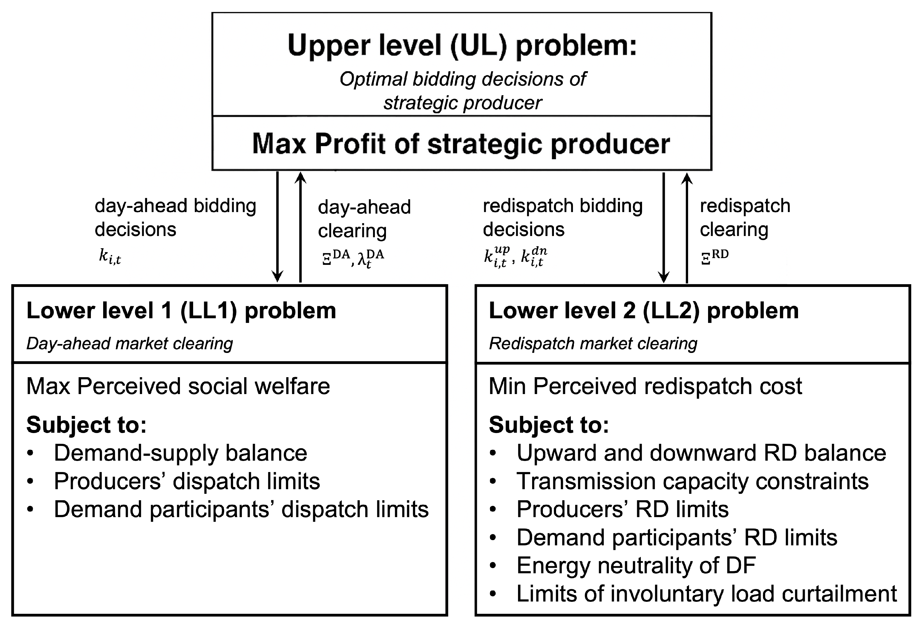
Figure 2.
Illustration of the 2-node system.
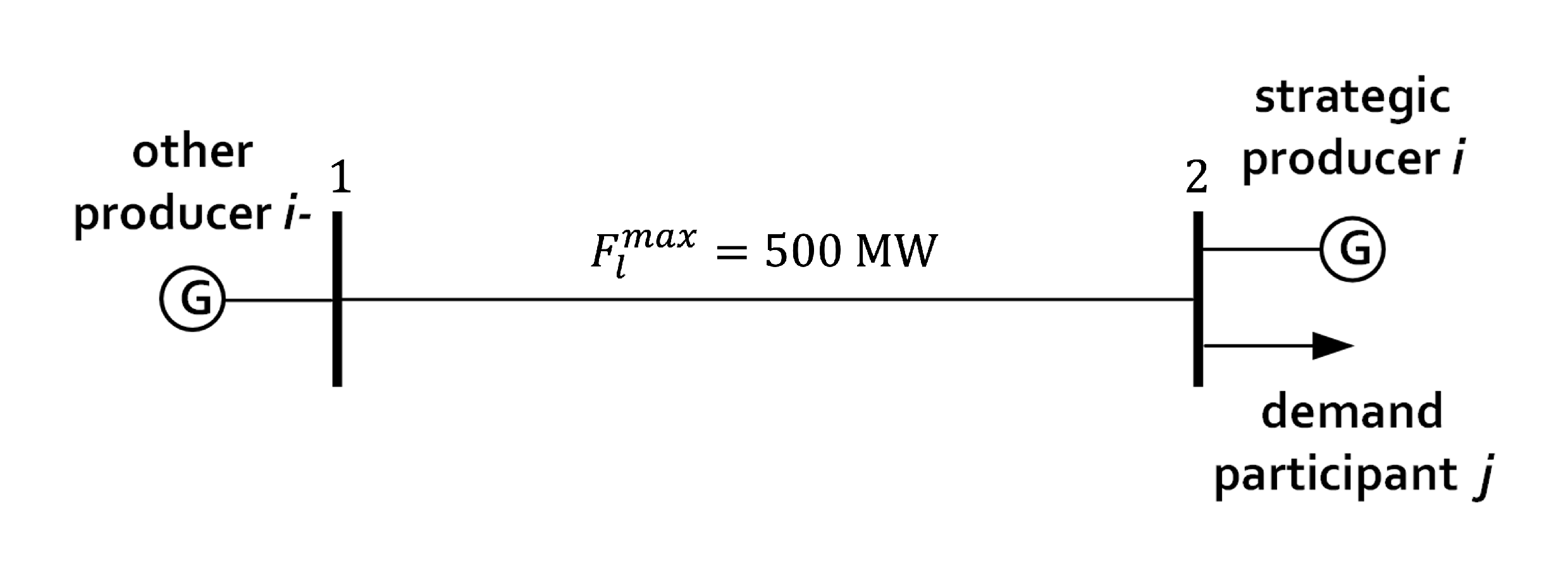
Figure 3.
Illustration of the modified IEEE RTS 24-node system.
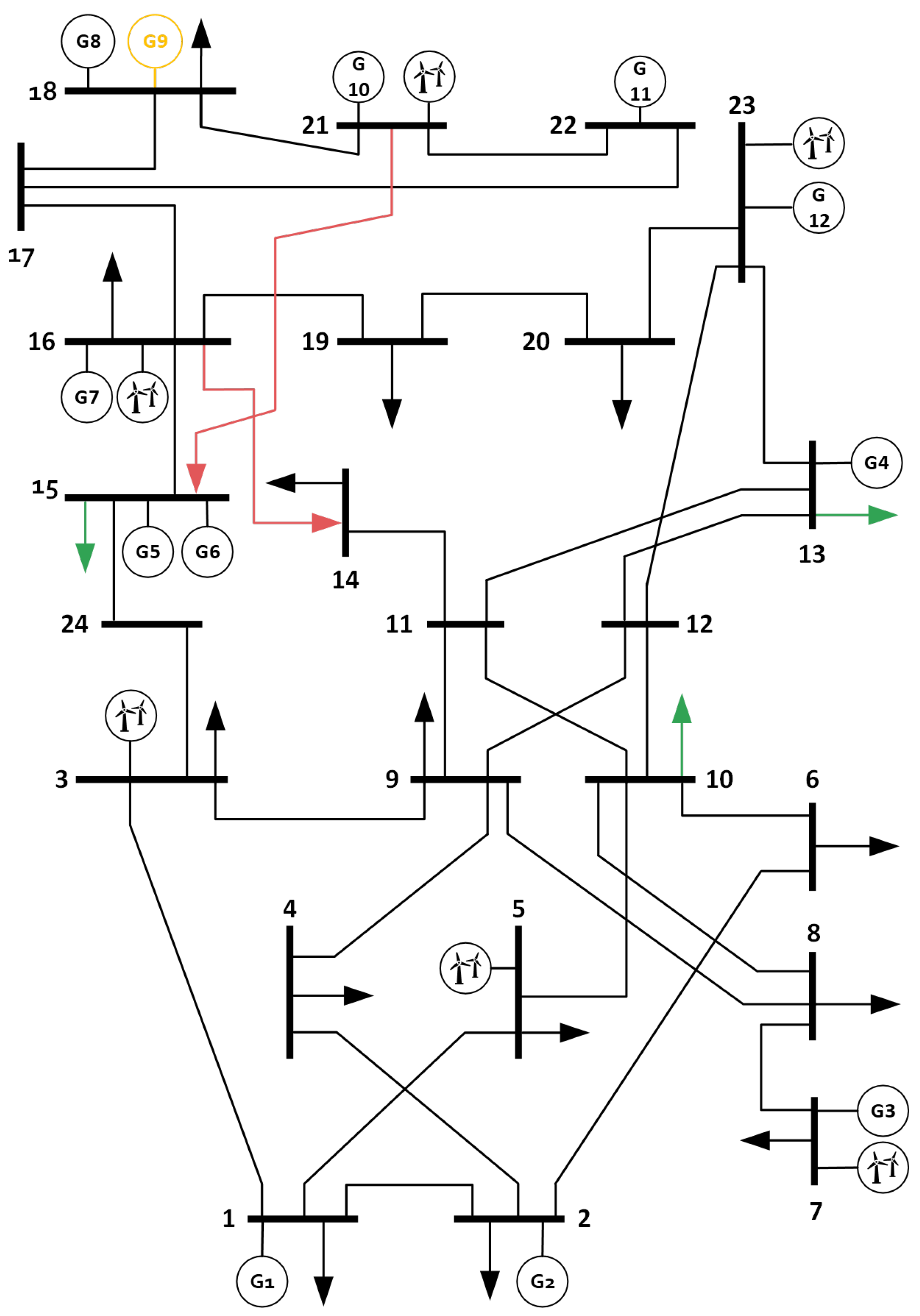
Figure 4.
Day-ahead market clearing under the scenario Strategic (same in the scenario Strategic + DF).
Figure 4.
Day-ahead market clearing under the scenario Strategic (same in the scenario Strategic + DF).
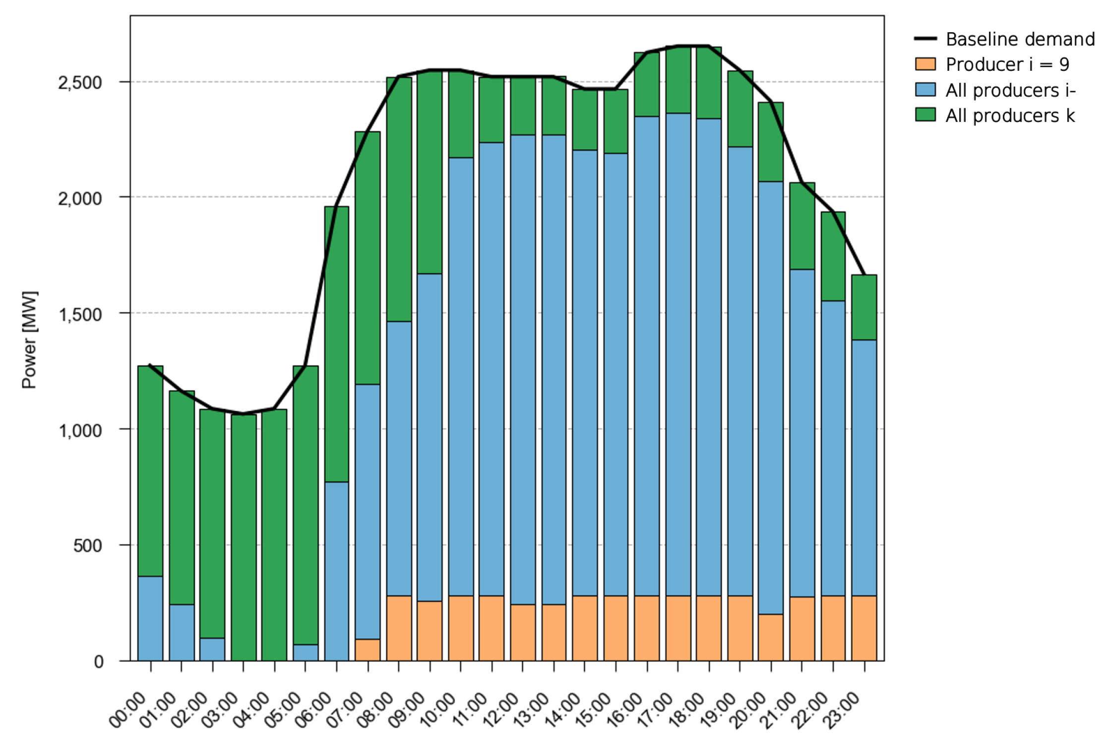
Figure 5.
Hourly congestion extent for different lines under the scenarios Benchmark and Strategic.
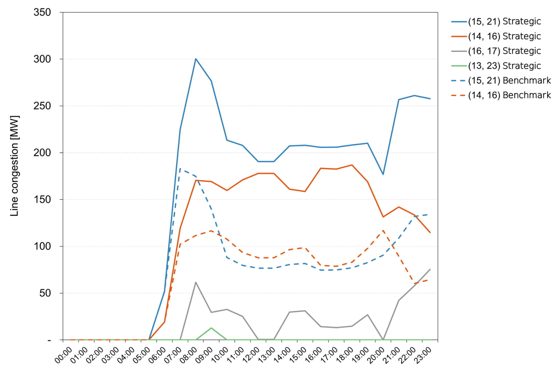
Figure 6.
Redispatch market activations under the scenarios Strategic (left) and Strategic + DF (right).
Figure 6.
Redispatch market activations under the scenarios Strategic (left) and Strategic + DF (right).
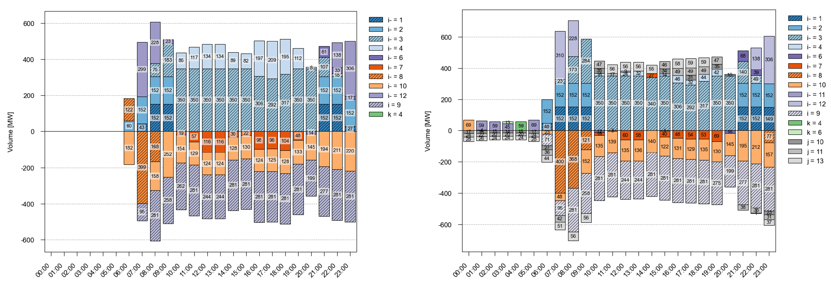
Table 1.
Summary of Existing Literature on Inc-Dec Gaming.
| Paper | Model | Examined Network | RD Participants | Time Frame | Time-Coupling |
|---|---|---|---|---|---|
| [12] | Analytical | No specific network | Producers | Single-period | No |
| [13,14] | Analytical | 2-node | Producers | Single-period | No |
| [15] | EPEC | No specific network | Producers | Single-period | No |
| [16] | EPEC | 24-node | Producers | Single-period | No |
| [17] | MPEC | 3-node | Producers | Single-period | No |
| This paper | MPEC | 24-node | Prod. and Demand-Side | Multi-period | Yes |
Table 2.
Producers’ parameters in the 2-node system.
| Producer i | Producer | |
|---|---|---|
| Marginal cost [£/MWh] | 10 | 15 |
| Maximum power [MW] | 1,200 | 1,200 |
Table 3.
Demand parameters in the 2-node system.
| t = 1 | t = 2 | |
|---|---|---|
| Marginal benefit [£/MWh] | 10,000 | |
| Upward discomfort cost [£/MWh] | 0.5 | 1 |
| Downward discomfort cost [£/MWh] | 1 | 0.5 |
| Maximum baseline power [MW] | 1,000 | 400 |
| VoLL [£/MWh] | 16,050 | |
Table 4.
System Outcome in 2-Node Case Study.
| Scenario | Benchmark | Strategic | Strategic + DF | |||
|---|---|---|---|---|---|---|
| Period | ||||||
| [MW] | 1,000 | 400 | 0 | 400 | 0 | 400 |
| [MW] | 0 | 0 | 500 | 0 | 420 | 80 |
| [MW] | 0 | 0 | 0 | 0 | 0 | 0 |
| [MW] | 0 | 0 | 1,000 | 0 | 1,000 | 0 |
| [MW] | 0 | 0 | 0 | 0 | 0 | 0 |
| [MW] | 0 | 0 | 500 | 0 | 500 | 0 |
| [MW] | 1,000 | 400 | 1,000 | 400 | 1,000 | 400 |
| [MW] | – | – | – | – | 80 | 0 |
| [MW] | – | – | – | – | 0 | 80 |
| [£/MW] | 10 | 10 | 15 | 15 | 15 | 15 |
| System costs [£] | ||||||
| DA | 10,000 | 4,000 | 15,000 | 6,000 | 15,000 | 6,000 |
| RD | 0 | 0 | 5,000 | 0 | 3,040 | 1,240 |
| Total | 10,000 | 4,000 | 20,000 | 6,000 | 18,040 | 7,240 |
| Daily total | 14,000 | 26,000 | 25,280 | |||
Table 5.
Strategic Producer’s Outcome in 2-Node Case Study.
| Scenario | Benchmark | Strategic | Strategic + DF | |||
|---|---|---|---|---|---|---|
| Period | ||||||
| 1.00 | 1.00 | 1.50 | 1.50 | 1.50 | 1.50 | |
| – | – | 2.50 | – | 2.50 | 1.50 | |
| – | – | – | – | – | – | |
| Revenues and costs [£] | ||||||
| Revenue DA | 10,000 | 4,000 | 0 | 6,000 | 0 | 6,000 |
| Cost DA | 10,000 | 4,000 | 0 | 4,000 | 0 | 4,000 |
| Revenue RD | 0 | 0 | 12,500 | 0 | 10,500 | 1,200 |
| Cost RD | 0 | 0 | 5,000 | 0 | 4,200 | 800 |
| Profit | 0 | 0 | 7,500 | 2,000 | 6,300 | 2,400 |
| Daily profit | 0 | 9,500 | 8,700 | |||
Table 6.
Hourly results in the large-scale case study. Left: day-ahead (DA) outcomes (, , ), which are identical in Strategic (S) and Strategic + DF (S+DF). Right: redispatch (RD) outcomes (, , ) shown separately for S and S+DF. and denote DA and RD profits, respectively.
Table 6.
Hourly results in the large-scale case study. Left: day-ahead (DA) outcomes (, , ), which are identical in Strategic (S) and Strategic + DF (S+DF). Right: redispatch (RD) outcomes (, , ) shown separately for S and S+DF. and denote DA and RD profits, respectively.
| t | [MW] | [£] | ||||||||
|---|---|---|---|---|---|---|---|---|---|---|
| [MW] | [£/MW] | [£] | S | S+DF | S | S+DF | S | S+DF | ||
| 00:00 | – | 0 | 5.47 | 0 | – | – | 0 | 0 | 0 | 0 |
| 01:00 | – | 0 | 0.50 | 0 | – | – | 0 | 0 | 0 | 0 |
| 02:00 | – | 0 | 0.50 | 0 | – | – | 0 | 0 | 0 | 0 |
| 03:00 | – | 0 | 0.00 | 0 | – | – | 0 | 0 | 0 | 0 |
| 04:00 | – | 0 | 0.00 | 0 | – | – | 0 | 0 | 0 | 0 |
| 05:00 | – | 0 | 0.50 | 0 | – | – | 0 | 0 | 0 | 0 |
| 06:00 | – | 0 | 6.02 | 0 | – | – | 0 | 0 | 0 | 0 |
| 07:00 | 0.40 | 95 | 10.52 | -1,518 | 0.23 | 0.21 | 95 | 95 | 1,940 | 2,001 |
| 08:00 | 0.40 | 281 | 10.52 | -4,490 | 0.23 | 0.23 | 281 | 281 | 5,738 | 5,738 |
| 09:00 | 0.43 | 258 | 11.32 | -3,916 | 0.25 | 0.23 | 258 | 258 | 5,134 | 5,268 |
| 10:00 | 0.70 | 281 | 18.52 | -2,242 | 0.25 | 0.25 | 262 | 281 | 5,214 | 5,592 |
| 11:00 | 0.70 | 281 | 18.52 | -2,242 | 0.32 | 0.32 | 281 | 281 | 5,047 | 5,047 |
| 12:00 | 0.78 | 244 | 20.70 | -1,415 | 0.32 | 0.32 | 244 | 244 | 4,382 | 4,382 |
| 13:00 | 0.78 | 244 | 20.70 | -1,415 | 0.32 | 0.32 | 244 | 244 | 4,382 | 4,382 |
| 14:00 | 0.70 | 281 | 18.52 | -2,242 | 0.32 | 0.32 | 281 | 281 | 5,047 | 5,047 |
| 15:00 | 0.70 | 281 | 18.52 | -2,242 | 0.32 | 0.25 | 281 | 281 | 5,047 | 5,592 |
| 16:00 | 0.78 | 281 | 20.70 | -1,630 | 0.32 | 0.32 | 281 | 281 | 5,047 | 5,047 |
| 17:00 | 0.78 | 281 | 20.70 | -1,630 | 0.32 | 0.32 | 281 | 281 | 5,047 | 5,047 |
| 18:00 | 0.78 | 281 | 20.70 | -1,630 | 0.32 | 0.32 | 281 | 281 | 5,047 | 5,047 |
| 19:00 | 0.70 | 281 | 18.52 | -2,242 | 0.32 | 0.25 | 281 | 275 | 5,047 | 5,473 |
| 20:00 | 0.70 | 199 | 18.52 | -1,588 | 0.25 | 0.25 | 199 | 199 | 3,960 | 3,960 |
| 21:00 | 0.43 | 277 | 11.32 | -4,205 | 0.25 | 0.25 | 277 | 277 | 5,513 | 5,513 |
| 22:00 | 0.40 | 281 | 10.52 | -4,490 | 0.25 | 0.25 | 281 | 281 | 5,592 | 5,592 |
| 23:00 | 0.40 | 281 | 10.52 | -4,490 | 0.25 | 0.23 | 281 | 281 | 5,556 | 5,738 |
Table 7.
Results of IEEE 24-Node Case Study
| Scenario | Benchmark | Strategic | Strategic + DF |
|---|---|---|---|
| Producer 9 results | |||
| DA Profit [£] | 0 | -43,630 | -43,630 |
| RD Profit [£] | 0 | 82,738 | 84,465 |
| Total Profit [£] | 0 | 39,108 | 40,834 |
| System results | |||
| Congestion [MW] | 3,399 | 7,049 | 7,049 |
| DA cost [£] | 748,058 | 706,372 | 706,372 |
| RD cost [£] | 39,284 | 81,228 | 74,981 |
| Total cost [£] | 787,342 | 787,599 | 781,353 |
Disclaimer/Publisher’s Note: The statements, opinions and data contained in all publications are solely those of the individual author(s) and contributor(s) and not of MDPI and/or the editor(s). MDPI and/or the editor(s) disclaim responsibility for any injury to people or property resulting from any ideas, methods, instructions or products referred to in the content. |
© 2025 by the authors. Licensee MDPI, Basel, Switzerland. This article is an open access article distributed under the terms and conditions of the Creative Commons Attribution (CC BY) license (http://creativecommons.org/licenses/by/4.0/).
Copyright: This open access article is published under a Creative Commons CC BY 4.0 license, which permit the free download, distribution, and reuse, provided that the author and preprint are cited in any reuse.


