Submitted:
12 November 2025
Posted:
14 November 2025
You are already at the latest version
Abstract
This study estimated peanut (Arachis hypogaea L.) leaf area index (LAI), a critical vegetation parameter, using spectral bands and vegetation indices (VIs) derived from PlanetScope (~3m) imagery by comparing Random Forest (RF), eXtreme Gradient Boosting (XGBoost), and Partial Least Squares Regression (PLSR) algorithms. Most VIs exhibited strong relationships with LAI but showed saturation when LAI reached 3 m²/m². Thirteen VIs were individually evaluated for estimating LAI using the aforementioned machine learning and statistical algorithms, and the results showed that the best single predictors of LAI are: SR and RTVIcore (RF, R2 = 0.84, RMSE = 0.62 m2/m2); RTVIcore (XGBoost, R2 = 0.88, RMSE = 0.52 m2/m2); and RTVIcore and MSAVI (PLSR, R2 = 0.61, RMSE = 0.96 m2/m2). The top six ranked VIs were selected to calibrate the RF, XGBoost, and PLSR algorithms. The validation of the algorithms showed that the RF achieved the highest prediction accuracy (R2 = 0.844, RMSE = 0.858 m²/m², RRMSE = 25.17%), followed by XGBoost (R2 = 0.808, RMSE = 0.92 m²/m², RRMSE = 26.99%), while the PLSR showed relatively lower model accuracy (R2 = 0.76, RMSE = 0.983 m²/m², RRMSE = 28.85%). Further results demonstrate that VIs derived from spectral bands provide superior model accuracy in estimating peanut LAI compared to the use of spectral bands alone. Overall, the presented results are significant for future crop monitoring using RF to reduce overreliance on multiple models for peanut LAI.
Keywords:
LAI
; PlanetScope
; spectral bands
; vegetation indices
; machine learning algorithms
1. Introduction
Projected global population growth necessitates optimized crop yields to ensure food security amidst increasing climate-driven extreme weather. Monitoring crop development with high-resolution satellite Earth Observation data supports informed, timely agricultural decisions such as precise timing of fertilizer applications (Radočaj et al., 2022; Yang et al., 2022; Zhai et al., 2025), irrigation scheduling (Ben Asher et al., 2013; Belaqziz et al., 2021), tracking diseases and pests (Zhang et al., 2019; Abd El-Ghany et al., 2020; Ennouri et al., 2020), weed control (Huang et al., 2018; Roslim et al., 2021), and crop yield prediction (Wang et al., 2018a; Ali et al., 2022). Leaf Area Index (LAI), defined as one half the total green leaf area per unit ground surface area (Chen & Black, 1992), serves as a key indicator of vegetation photosynthetic potential, canopy structure, and energy exchange processes. In addition, it is an important indicator of monitoring overall plant health and estimating yield (Xiao et al., 2011). LAI can also be used indirectly as an input parameter in ecosystem productivity and crop growth simulation models (Myneni et al., 2002; Casa et al., 2012).
Traditionally, LAI can be estimated using ground-based methods, including direct and indirect approaches. Direct methods involve a destructive sampling approach, typically requiring harvesting of leaves or the collection of leaf litter (Fang et al., 2019). Although the direct measurements of LAI are considered to be the most accurate, there are tedious and labor intensive, and nearly impossible in large-scale agricultural fields. Therefore, direct methods are suitable only for small-scale applications and a limited number of measurements throughout the plant growth cycle (Behera et al., 2010). On the contrary, indirect approaches estimate LAI using allometric models by establishing relationships with other measurable plant attributes such as plant height and canopy area (Jonckheere et al., 2005). Other indirect methods of measuring LAI include using optical proximal sensors such as LAI-2000 Plant Canopy Analyzer (LI-COR, Inc., Nebraska, USA) (Liang et al., 2015), Digital Hemispherical Photos (Kross et al., 2015), licensed PocketLAI Smart-App (Cassandra Tech S.r.l) (Confalonieri et al., 2013; Campos-Taberner et al., 2016; Caballero et al., 2022), and VitiCanopy mobile App (University of Adelaide, Australia) (Ilniyaz et al., 2022; Ekwe et al., 2024). Both direct and indirect approaches are complementary, as indirect methods still require calibration using direct measurements (Behera et al., 2010). The application of these proximal sensors for accurate LAI monitoring has been documented in the literature. For example, Stroppiana et al. (2006) compared paddy rice LAI estimates from LAI-2000 with destructive LAI measurements and showed there were strongly correlated (R2>0.8), however, relationship reduces when LAI values are below one (R2<0.6). Among the indirect methods, Digital Hemispherical Photography (DHP) has been extensively employed to estimate LAI due to its non-destructive nature, relatively low cost, and accuracy (Jonckheere et al., 2004; Kross et al., 2015). However, the processing of captured crop canopy images to estimate LAI can be tedious, and requires high expert knowledge, particularly when using the CanEye software.
The increasing availability of high-tech sensors and computational capability of smartphone devices have paved the way for the development of low-cost Apps for indirect LAI monitoring. For example, Francone et al. (2014) compared PocketLAI and AccuPAR and showed overall good performances for the apps, with root mean square error of 0.41, 0.49 and 0.96 m2 m−2 for grassland, maize and giant reed respectively. The availability of a low-cost smartapp capable of providing absolute LAI estimates in real time, without the need for time-consuming post-processing or parameter calibration, represents a practical and user-friendly tool for operational applications in viticulture, benefiting various agricultural stakeholders (Orlando et al., 2016). Recently, VitiCanopy App was developed to accurately estimate the canopy vigor and porosity in vine canopies (De Bei et al., 2016). Similar to DHP technique, the VitiCanopy app acquires images from below the canopy and automatically processes them to estimate LAI, following a similar approach by PocketLAI smartapp. However, the VitiCanopy user is required to define the gap fraction threshold representing the proportion of image pixels corresponding to sky prior to taking measurements (Orlando et al., 2016). Previous studies have shown that LAI estimates from VitiCanopy App demonstrated good agreement with estimates measured by LAI-2000 Plant Canopy Analyzer (De Bei et al., 2016). However, the application of this low-cost approach for LAI monitoring has received limited attention in crop monitoring studies (e.g., Ekwe et al., 2024).
Satellite Earth Observation data has been mostly used in past LAI estimation studies due to its time, cost, and labor savings for large crop areas. Predominantly, vegetation indices (VIs) derived from optical remote sensing data have been widely used to estimate crop LAI (Nguy-Robertson et al., 2012; Kross et al., 2015). VIs describe mathematical combinations, ratios (or normalization) of optical spectral reflectance data, and can help in mitigating the influence of atmospheric, bidirectional reflectance and soil background effects (Marshall & Thenkabail, 2015; Kamal et al., 2016). Overall, distinct VIs exhibit varying sensitivity to LAI estimates. For example, the traditional Normalized Difference Vegetation Index (NDVI) has shown a strong relationship with LAI, however, it saturates at medium to high LAI values (Nguy-Robertson et al., 2012; Kross et al., 2015). Nguy-Robertson et al. (2012) reported that NDVI is sensitive to low LAI values (LAI < 2-3 m2/m2) and saturates at LAI greater than 3 m2/m2. Similarly, Kross et al. (2015) demonstrated that NDVI saturates when LAI is approximately at 6 m2/m2. Simple ratio (SR), modified triangular vegetation index 2 (MTVI2) and cumulative MTVI2 have shown improved sensitivity at medium to high LAI values (Haboudane, 2004; Nguy-Robertson et al., 2012). Similarly, VIs that incorporate red-edge reflectance bands such as the Red-Edge Triangular Vegetation Index (RTVI) and the Modified Chlorophyll Absorption Ratio Index (MCARI2), have shown enhanced potential for accurate estimation of LAI at medium to high values (Kross et al., 2015). Additionally, several studies have examined various spectral vegetation indices that have demonstrated strong correlations with LAI estimation (Li et al., 2019; Du et al., 2022; Hussain et al., 2025). Du et al. (2022) showed that RGB-based VIs generated from UAV images were strongly correlated to maize LAI. A study by Li et al. (2019) established that the visible atmospherically resistant index (VARI) was the best for rice LAI estimation.
Accurate crop monitoring in precision agriculture relies on Earth observation data with sufficiently high spatial and temporal resolutions. The PlanetScope constellation, comprising Dove and SuperDove satellites, meets this demand by providing daily imagery at 3 m spatial resolution, including a red-edge band, with near-daily global land coverage. Spectral VIs derived from PlanetScope imagery have been successfully applied to estimate soybean yield (Amankulova et al., 2023), rice LAI (Serrano Reyes et al., 2023), peanut maturity (Souza et al., 2022; Barboza et al., 2025), and peanut and corn grain yield (Kpienbaareh et al., 2022; Li et al., 2022). However, despite its high spatial-temporal resolutions, PlanetScope imagery is limited by relatively low spectral resolution and higher sensitivity to cloud cover, which can impact its reliability for accurate LAI estimation under variable field conditions. Furthermore, its potential for estimating peanut LAI has not been thoroughly investigated, indicating a notable gap in current research. This study addresses this gap by evaluating the capability of PlanetScope data for monitoring peanut LAI. These limitations highlight the need to integrate advanced nonparametric machine learning and statistical methods to fully utilize PlanetScope data for accurate peanut LAI monitoring, which is the focus of the present study.
Machine learning (ML) and statistical algorithms are increasingly utilized in remote sensing literature to retrieve crop and vegetation growth indicators such as LAI. In nonparametric regression methods, ML algorithms are trained and validated using in situ data, enabling the establishment of relationships between spectral data and vegetation biophysical parameters of interest. Linear nonparametric algorithms such as the Partial Least Squares Regression (PLSR) algorithm have proven successful in previous studies for the estimation of LAI and biomass in winter wheat (Fu et al., 2013; Tao et al., 2020). However, linear nonparametric algorithms may not be the best candidates to handle complex data with nonlinear relationships (Verrelst et al., 2015). ML algorithms are best suited for limited sample sizes and noisy variables (Kganyago et al., 2021), and have demonstrated superiority in estimating crop parameters when compared to parametric regression algorithms (Fu et al., 2021; Bahrami et al., 2022). For example, Kganyago et al. (2021) compared random forest (RF), sparse Partial Least Squares (sPLS), and Gradient Boosting Machine (GBM) for the estimation of LAI, leaf chlorophyll content (LCab), and canopy chlorophyll content (CCC) in maize, beans, and peanut crops, finding that RF outperformed both sPLS and GBM across all the three parameters. Reisi Gahrouei et al. (2020) applied Artificial Neural Network (ANN) and Support Vector Regression (SVR) models to estimate biomass and LAI in canola, corn, and soybeans, and found that SVR produced more accurate LAI and biomass estimates than ANN. Zhang et al. (2021) compared three modeling ML methods including partial least squares regression (PLSR), SVR, and extreme gradient boosting (XGBoost) for the estimation of winter wheat LAI using UAV hyperspectral images, and found that the XGBoost model using nine spectral bands yielded the best performance (R2 = 0.89, RMSE = 0.55, and relative percent deviation (RPD) = 2.29). Ghosh et al. (2022) used the Gaussian Process Regression (GPR) algorithm to retrieve plant area index, wet biomass, and vegetation water content of wheat, canola, and soybean crops using C-band RADARSAT-2 data, and found that GPR achieved superior accuracy compared to other ML algorithms, particularly SVR and RF. ML methods offer the potential to incorporate expert prior knowledge and can integrate multiple predictor variables (e.g., spectral bands, VIs) to develop robust nonlinear-complex relationships; therefore, they are widely used for interpreting Earth Observation data for estimating crop yield indicators such as LAI.
This study examined two nonlinear ML (RF and XGBoost) and one linear nonparametric (PLSR) models to estimate peanut LAI using PlanetScope data over a rainfed agricultural field characterized by moderately scaled commercial farming practices. RF, an ensemble ML algorithm based on decision trees, is particularly effective for handling high-dimensional and nonlinear relationships between spectral variables and crop biophysical parameters, while being relatively insensitive to noise and overfitting (Belgiu & Drăguţ, 2016). XGBoost, a gradient boosting algorithm, is known for minimizing prediction errors by building decision trees to ensure higher model accuracy (Chen & Guestrin, 2016). The inclusion of PLSR in this study provides a statistical baseline for comparison; it effectively reduces multicollinearity among highly correlated predictor variables by projecting them into a reduced set of orthogonal latent variables (Wold et al., 2001). By exploring these models, this study aims to comprehensively evaluate the capabilities of both linear and nonlinear nonparametric models for estimating peanut LAI using PlanetScope spectral features. Additionally, evaluating these three algorithms in the context of peanut LAI estimation is important to reveal their relative performance under consistent tropical climatic conditions.
The specific objectives of this study are to: (1) investigate the relationships between LAI and PlanetScope-derived VIs, (2) identify the important spectral features (bands or VIs) with the highest predictive power for estimating peanut LAI, and (3) evaluate and compare the predictive performance of RF, XGBoost, and PLSR algorithms in estimating peanut LAI using PlanetScope data. These regression models have been explored in previous studies for estimating crop biophysical parameters from PlanetScope data for crop monitoring.
2. Data and Methods
2.1. Study Area Description
The smallholder farmer’s experimental study site is located in the tropical north-central region of the Federal Capital Territory (FCT), Abuja, Nigeria. The site covers an area of approximately 3,712.45m2 and is situated at the coordinates: latitude (8°56’58.92”N~8°57’0.054”N) and longitude (7°5’30.804”E~7°5’32.172E”) (Figure 1). The study area is largely covered by fertile alluvial soils that are clayey, loamy, and silty, providing ideal conditions for peanut crop cultivation. According to the Köppen climate classification system, the region experiences a tropical wet and dry climate (Aw). The weather in the region is primarily influenced by orographic features and the dynamic interaction between two dominant air masses: the tropical continental (cT) air mass and the tropical maritime (mT) air mass (Orisakwe et al., 2017). The region witnesses the rainy season between mid-March and October, which is important for peanut production. During the dry season around March, daytime temperatures in the region can reach up to 39 °C, whereas during the Harmattan period (December-January), nighttime temperatures can drop to as low as 17 °C (Ekwe et al., 2024). The optimal soil temperature for effective germination and vegetative growth of peanut ranges between 27 °C and 30 °C, while the ideal temperature for the reproductive growth phase lies between 24 °C and 27 °C; additionally, annual rainfall between 450mm and 1250mm is required for optimum growth and yield (Ajeigbe et al., 2015). The experimental site is well-known for its crop rotational cultivation of peanut, corn (Zea mays), and Bambara groundnuts (Vigna subterranea).
2.2. Experimental Design and In Situ Data Measurement
In the experimental field, peanut was manually cultivated under rainfed conditions using the medium-maturing variety Samnut-22, immediately after the onset of the rainy season on April 19, 2022 (Figure 2). Seeding was conducted along clearly defined ridges within the field, which covered a total area of 3,712.45 m². A total of 83 sampling points were randomly selected for in situ LAI measurements. LAI measurement was conducted using the Viticanopy Smart-App installed on Tecno Spark 5 Pro with Android operating system. In addition to LAI, the Viticanopy app also measures canopy porosity, and canopy growth, and it operates by capturing images from below the canopy, similar to Digital Hemispherical Photography (DHP) (Orlando et al., 2016). Further details regarding the description and configuration settings of the app can be found in De Bei et al. (2016). The Viticanopy Smart-app has been successfully tested and validated in previous studies for monitoring LAI and phenology in different crop and vegetation types, including vineyards (Pichon et al., 2020; Ilniyaz et al., 2022; Pagliai et al., 2022), orchards (Rouault et al., 2024), and groundnut (Ekwe et al., 2024).
Figure 1.
Geographical location and spatial layout of the peanut experimental site. Sampling points for LAI measurements, collected on 22 May 2022, are indicated by red dots (Source: Ekwe et al., 2024).
Figure 1.
Geographical location and spatial layout of the peanut experimental site. Sampling points for LAI measurements, collected on 22 May 2022, are indicated by red dots (Source: Ekwe et al., 2024).
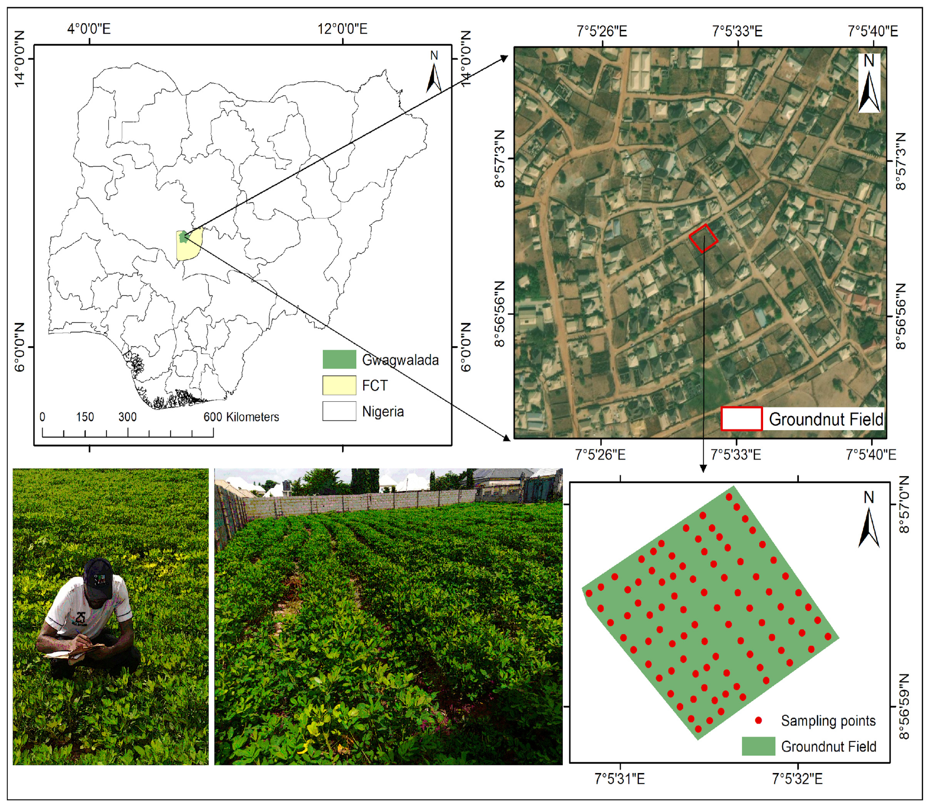
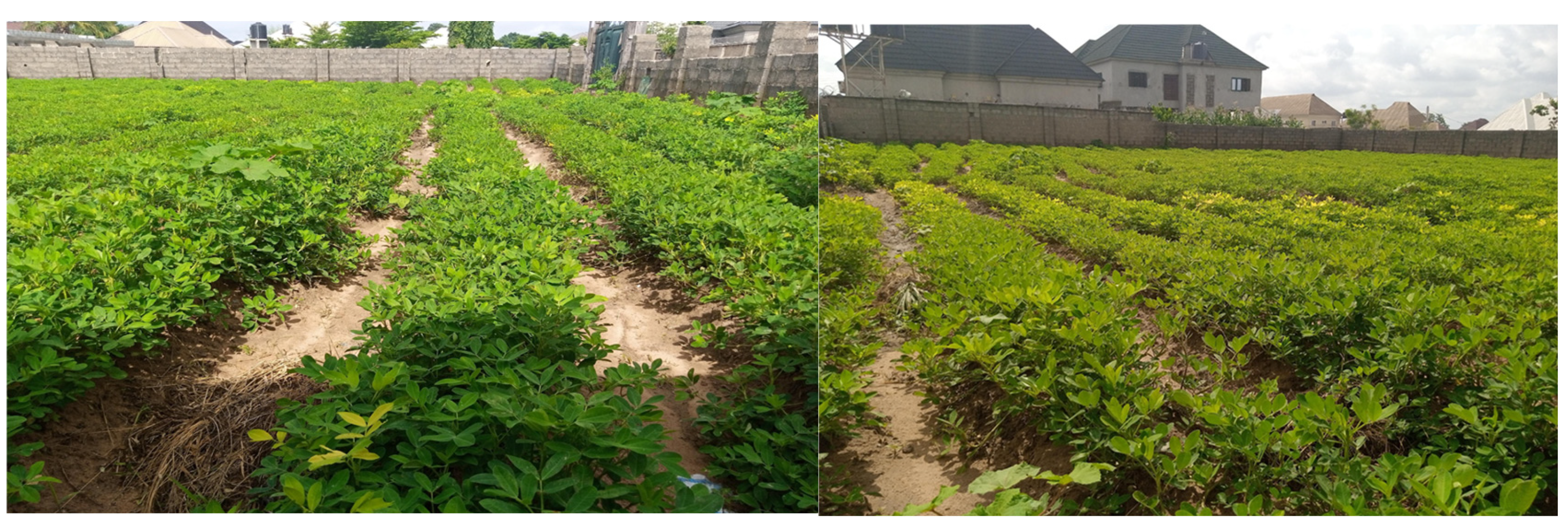
Figure 2.
Photos of the peanut experimental field captured on May 22, 2022.
2.3. Satellite Data
PlanetScope Imagery and Preprocessing
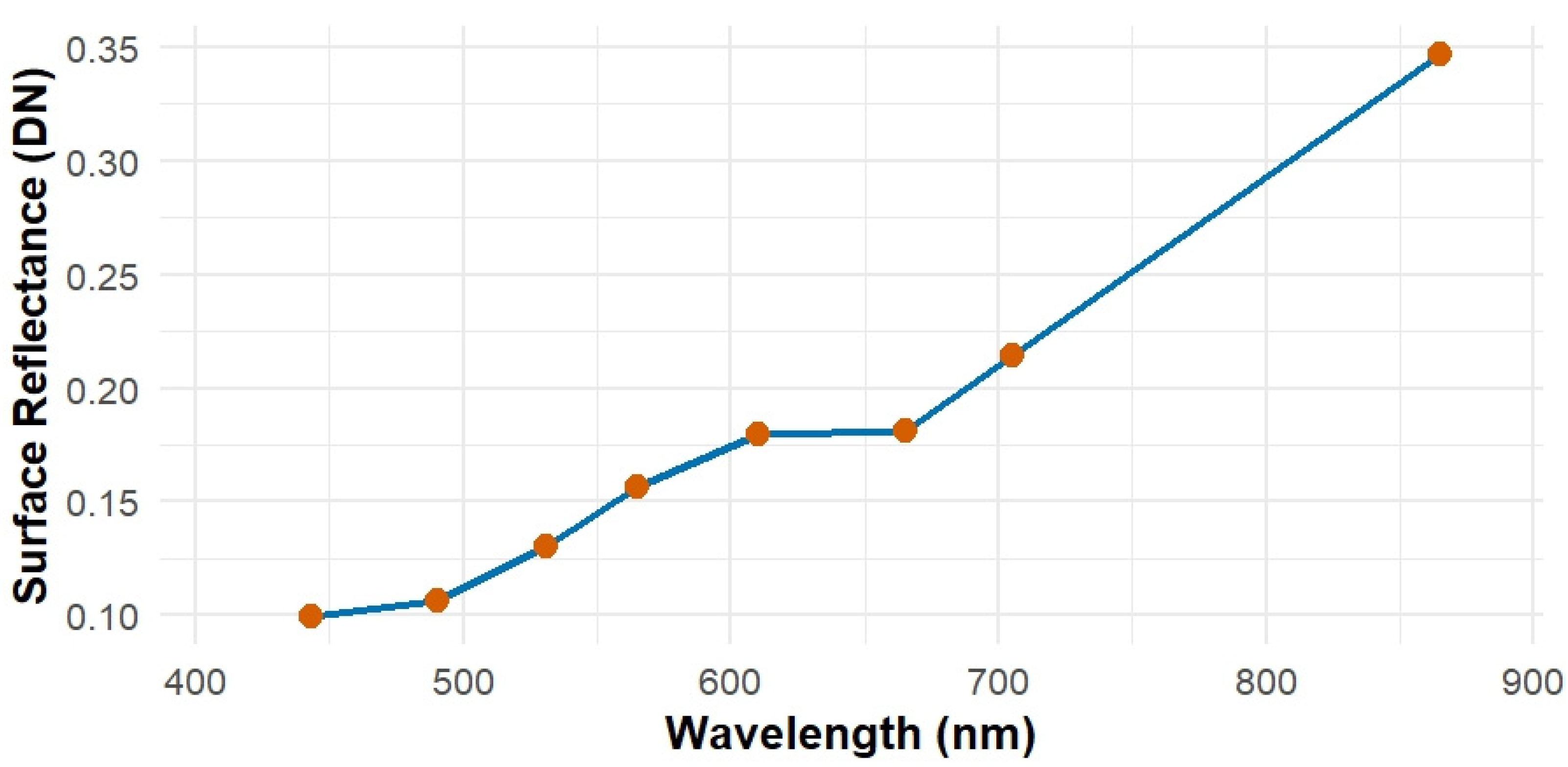
Cloud-free PlanetScope level-3 surface reflectance imagery collected on 22 May, 2022 was downloaded from the Planet Explorer website (https://www.planet.com/explorer/; accessed on October 25, 2024). In this study, the PSB.SD sensor, Dove CubeSat from the PS SuperDove series, was utilized. The PSB.SD instrument offers eight spectral bands, namely red-edge, red, green, green I, yellow, blue, coastal blue, and near infrared (NIR), with a spatial resolution of 3 m and a near-daily global revisit frequency. The PlanetScope orthorectified product was processed for geometric and radiometric corrections to account for Bottom-Of-Atmosphere (BOA) surface reflectance and projected into the UTM/WGS84 coordinate reference system (Planet Team, 2025). The spectral response of the peanut canopy captured by the PSB.SD sensor is presented in Figure 3, which revealed that peanut canopy exhibited higher reflectance in the near-infrared region (centered at 865 nm) and greater absorption in the blue band (centered at 490 nm).
Figure 3.
Spectral response of peanut canopy captured by PlanetScope across Coastal Blue, Blue, Green I, Green, Yellow, Red, Red-Edge, and Near-Infrared surface reflectances for the experimental site on May 22, 2022.
Figure 3.
Spectral response of peanut canopy captured by PlanetScope across Coastal Blue, Blue, Green I, Green, Yellow, Red, Red-Edge, and Near-Infrared surface reflectances for the experimental site on May 22, 2022.
2.4. Remote Sensing Variables
We used a total of thirteen VIs and five PlanetScope surface reflectance bands to estimate peanut LAI (Table 1). All the VIs were generated using the ‘Indices’ tool available within the ArcGIS Pro software environment (ESRI, Redlands Inc., CA, USA). We used the coordinates of each sampling location and retrieved all the matching VIs and bands using the ‘Extract Multi Values to Points’ function within the Spatial Analyst tools in ArcGIS Pro software.
2.5. Modeling Methods
Two ML (RF and XGBoost) and one linear nonparametric (PLSR) algorithms were chosen to guarantee robust and accurate LAI estimations using different algorithms. These models were selected based on their advantages and relevance for estimating LAI using PlanetScope-derived spectral reflectance bands and VIs. The selection of these algorithms enables a comprehensive evaluation of model performance and the identification of the most effective approach for predicting peanut LAI.
RF is a non-parametric ensemble learning method derived from the principles of CART (classification and regression trees), and it encompasses various trees that are trained using bagging and random variable selection approach (Breiman, 2001). The RF algorithm is robust to outliers and noise (Gleason & Im, 2012), making it well-suited for handling overfitting and complex datasets. Previous studies have demonstrated its accuracy in estimating vegetation biophysical parameters such as LAI (Beckschäfer et al., 2014; Li et al., 2017; Srinet et al., 2019; Shao et al., 2021; De Magalhães & Rossi, 2024). In this study, the Variable Selection Using Random Forests (VSURF) was used to determine the most important predictor variables for predicting the peanut LAI. RF modeling was performed using the “randomForest” package in base R. In the RF model, default hyperparameters were applied, with the number of trees (ntree) set to 500 and the number of features considered at each split (mtry) set to 3. Several studies have identified 500 trees as an optimal number for the RF model, as increasing the number of trees beyond this threshold does not lead to significant improvements in prediction accuracy (Belgiu & Drăguţ, 2016). We deployed the built-in importance() function in the ‘randomForest’ package to provide important predictor variables using the Percent Increase in Mean Squared Error (%IncMSE) metric (Breiman, 2001; Varela et al., 2021). The higher a variable’s %IncMSE value is, the more important the predictor variable is (Kaveh et al., 2023).
XGBoost is a powerful ensemble learning model that integrates gradient boosting with advanced regularization approaches to improve predictive performance (Anees et al., 2024). It employs an iterative learning process in which errors from previous iterations are incorporated to enhance the performance of subsequent iterations, thereby improving overall model accuracy. Through regularization, XGBoost algorithm reduces overfitting, handles missing data, and requires less training and prediction time, making it highly robust for large-scale data (Chen & Guestrin, 2016). XGBoost model was chosen for its exceptional performance in crop LAI mapping, as evidenced by prior research (Geng et al., 2021; Liu et al., 2021; Zhang et al., 2022). In this study, the model was fine-tuned using different hyperparameters, including the number of boosting rounds (nrounds = 500), learning rate (eta = 0.1), maximum depth of each decision tree (max_depth = 6), and the evaluation metric (eval_metric) was set to root mean square error. XGBoost modeling was performed using the “xgboost” package in base R. We used the built-in xgb.importance() function in the xgboost package to provide important predictor variables using the Gain% feature importance metric.
PLSR is a widely applied multivariate statistical technique commonly employed for developing predictive models, particularly in scenarios where the explanatory variables are numerous, highly correlated, and exhibit multicollinearity (Maimaitijiang et al., 2020). It reduces dimensionality and noise by transforming collinear input features into a smaller set of uncorrelated latent variables through component projection; however, interpreting the coefficients can be challenging (Geladi & Kowalski, 1986). Prior research has shown PLSR to be one of the effective nonparametric linear methods for estimating LAI (Li et al., 2014; Kiala et al., 2016; Panigrahi & Das, 2021). In this study, the PLSR modeling was performed using the “pls” package in base R with five PLS components, and the model was fitted with the kernel algorithm. For the PLSR modeling, the Variable importance in projection (VIP) function (Hastie et al., 2005) was used to select the important features.
These RF, XGBoost, and PLSR algorithms provide robust and reliable estimation of crop biophysical parameters such as LAI, with their respective advantages and limitations summarized in Table 2.
2.6. Statistical Evaluation
Data partitioning was conducted using the “createdatapartition()” function from the caret package in base R, allocating 70% of the data for training and 30% for validation. We assessed the relationship between LAI and spectral features using the cor() function in R, quantified as Pearsons’s correlation coefficient (R). The assessment of model performance was performed by adopting the root mean square error (RMSE), relative RMSE (RRMSE%), and coefficient of determination (R2). The equations of these evaluation metrics were expressed as follows:
where is the measured LAI, is the estimated LAI, and are the average measured and estimated LAI, respectively; and n is the number of observations used for model validation.
2.7. Generation of LAI Prediction Maps
To create the peanut LAI prediction maps, raster layers of the most important VIs were needed. The raster layers of the VIs were generated using the “indices” tools in ArcGIS Pro software (ESRI, Redlands Inc., CA, USA). The top six VIs, identified based on their feature importance for the RF, XGBoost, and PLSR algorithms respectively, were selected to generate the final LAI prediction maps. In the base R, the “library(raster)”, “library(rgdal)”, and “library(rasterVis)” were utilized to create the final LAI prediction maps. The input raster layers (i.e., the VIs) were stacked using the “stack ()” function, and the “raster::predict ()” tool was deployed to predict LAI using the stacked layers and each algorithm. The outputs were exported as .Geotiff files into the ArcGIS Pro software to create the final LAI prediction maps.
3. Results and Discussion
3.1. The Descriptive Statistics of Peanut LAI Measurements
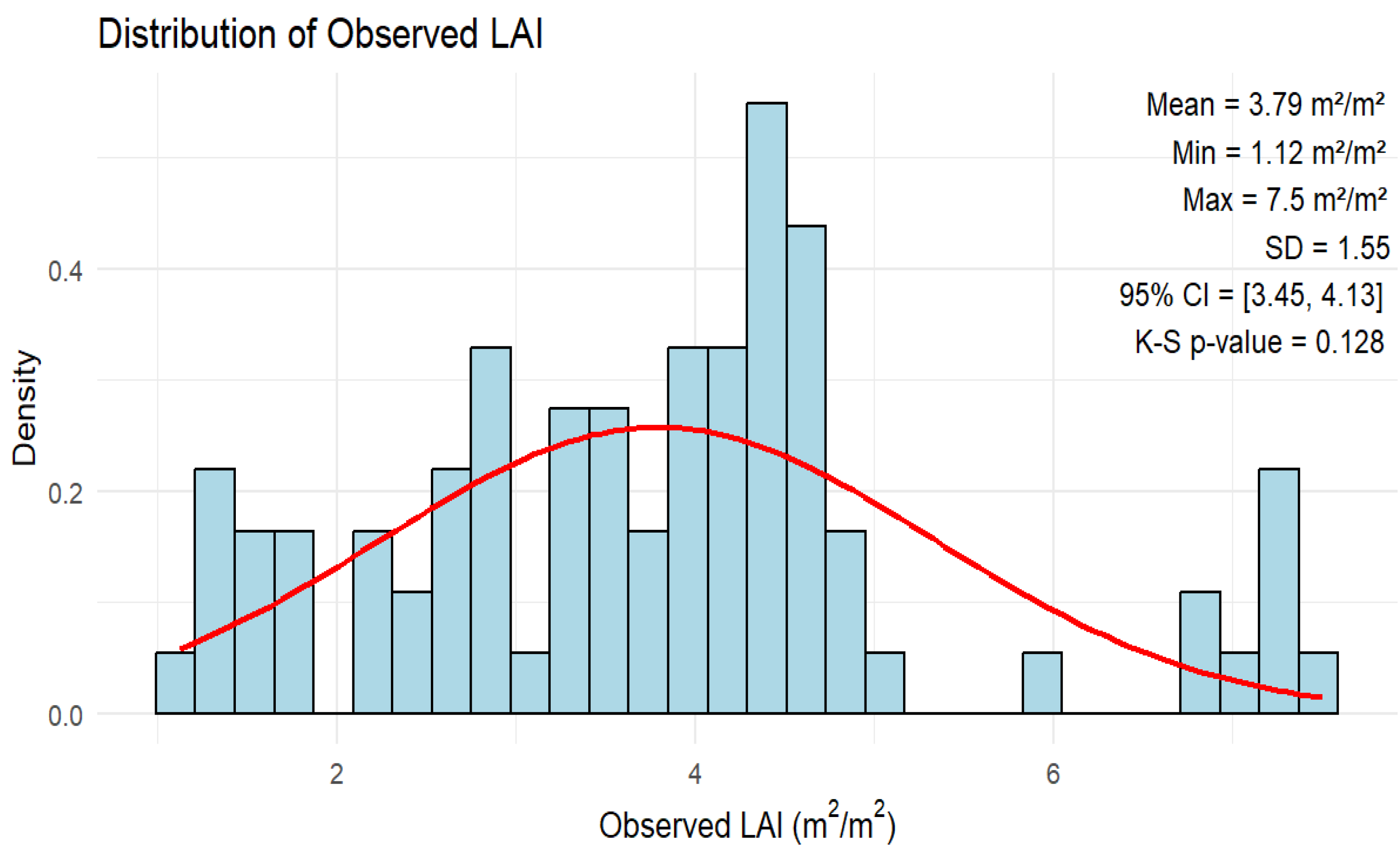
The normality of the LAI data was assessed using the Kolmogorov–Smirnov (K–S) test with a p-value of 0.128 (Figure 4). The distribution curve showed that LAI did not significantly deviate from a normal distribution. Although it follows normal distribution, it is not a critical factor to consider when assessing the performance of nonparametric algorithms. The observed peanut LAI ranged from a minimum of 1.12 m2/m2 to a maximum of 7.5 m2/m2, with an average value of 3.79 m2/m2, indicating moderate to dense canopy (Figure 4). A study by Sarkar et al. (2021) reported that the measured average peanut LAI in 2017 ranged from 0.8 to 2.6, and the values in 2019 varied from 1.5 to 5.8 with mean LAI values of 1.6 and 3.7 in 2017 and 2019, respectively. These values are consistent with the range of in situ mean peanut LAI values observed in the present study.
3.2. Assessment of Vegetation Indices for the Estimation of Peanut LAI
All the PlanetScope-derived VIs showed sensitivity across the full range of peanut LAI values, from 1.12 m²/m² to 7.5 m²/m², with different data samples clustered around the best fit line and r2 ranging between 0.25 and 0.61 (Figure 5). Among the thirteen VIs, MSAVI and RTVIcore captured the LAI, with the highest coefficient of determination (r2 = 0.61), followed by NDVI and SAVI (r2 = 0.59). The findings demonstrate that NDVI and SAVI exhibit saturation at LAI values exceeding 3 m²/m², limiting their effectiveness for estimating higher LAI values. Previous studies have demonstrated strong correlations between measured LAI and NDVI derived from MODIS data (Nguy-Robertson et al., 2012) and RapidEye imagery (Kross et al., 2015); however, Nguy-Robertson et al. (2012) found NDVI to be more sensitive to low LAI values (particularly < 2–3 m²/m²) with saturation occurring at medium to high LAI (> 3 m²/m²), while Kross et al. (2015) similarly observed NDVI saturation at LAI levels around 6 m²/m², which are consistent with the findings from this study. The MTVI2 showed a weak relationship with LAI, with the lowest coefficient of determination (r2 = 0.25). Sun et al. (2021) found that MTVI2 derived from Medium Resolution Imaging Spectrometer (MERIS) satellite data was strongly correlated with crop LAI; however, in this study, MTVI2 proved less effective for estimating peanut LAI, as many of its data points clearly deviated from the 1:1 fit line. We applied Pearson’s correlation analysis between LAI and all thirteen VIs, and results showed that gNDVI, NDVI, NDVIre, SAVI, and TSAVI exhibit strong relationships with LAI (r > 0.75) (Figure 6), but these indices showed some saturation when LAI reached 3 m²/m² (Figure 5c,f,g,I,l). These observed sensitivities align with the findings of Nguy-Robertson et al. (2012), who also reported saturation for LAI values at 3 m²/m². The MSAVI and RTVIcore exhibited strong relationships with LAI and showed no saturation across the full range of LAI values (Figure 4d,h). These results support the findings of Kross et al. (2015), who reported that RTVIcore did not exhibit saturation across the full range of LAI values. For MSAVI, this is consistent with the results of Din et al. (2017), who demonstrated that MSAVI showed no saturation when rice LAI exceeded 3 m²/m². The findings of this study indicate that MSAVI and RTVIcore are suitable for monitoring peanut with dense canopies.
Figure 4.
Descriptive statistics of observed peanut LAI.
3.3. Relationships Between Observed and Predicted Peanut LAI
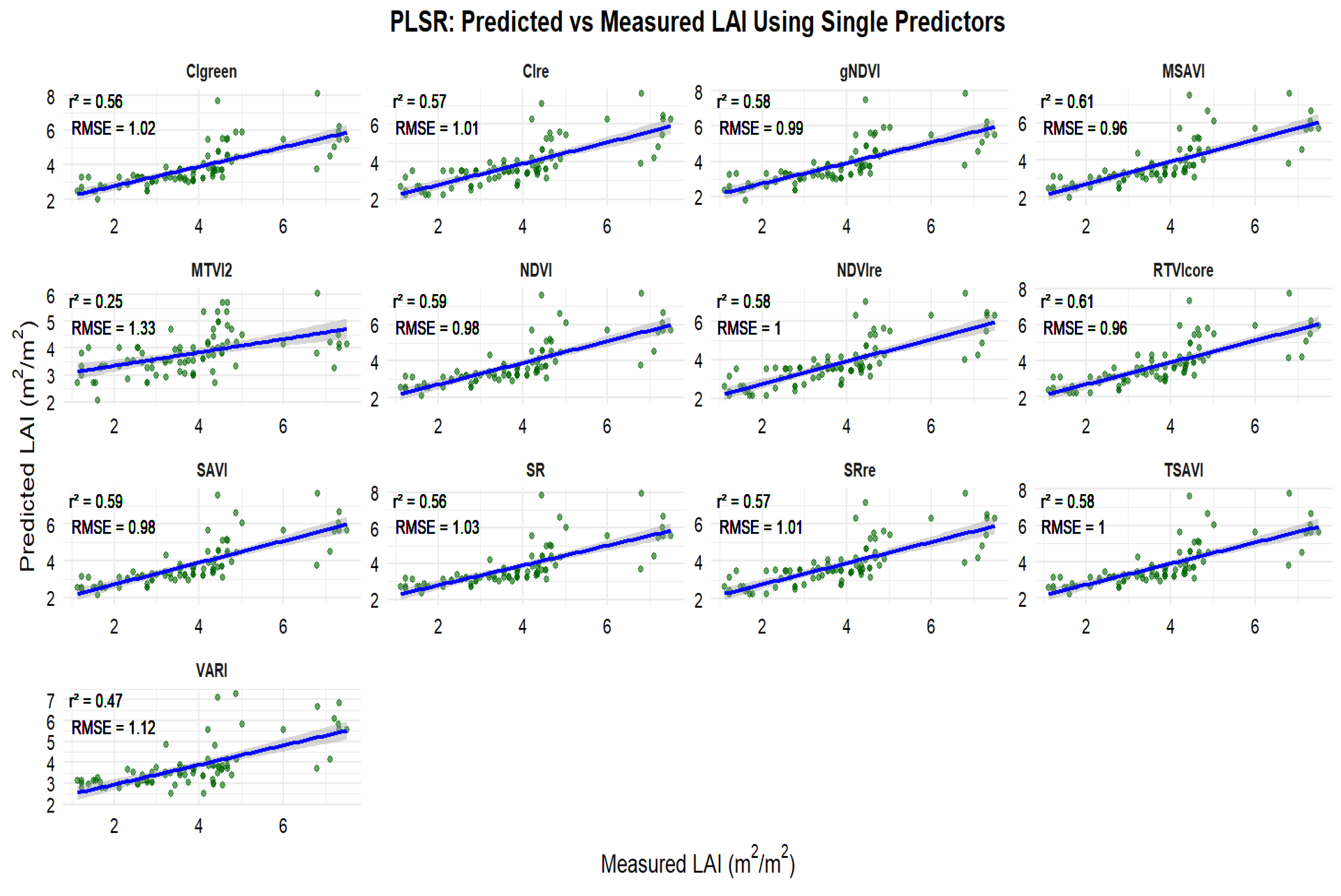
Figure 7, Figure 8 and Figure 9 show the relationship between the measured and the predicted LAI for each of the thirteen VIs based on RF, XGBoost, and PLSR modeling, respectively. The RMSE values that were generated by comparing the predicted with the measured LAI ranged from 0.62 m2/m2 (RTVIcore and SR) to 1.1 m2/m2 (MTVI2) for RF; 0.52 m2/m2 (RTVIcore) to 1.09 m2/m2 (MTVI2) for XGBoost; and 0.96 m2/m2 (RTVIcore and MSAVI) to 1.33 m2/m2 (MTVI2) for PLSR. The results showed poor agreement between measured and estimated LAI using the MTVI2, especially when measured LAI was greater than 3 m2/m2. This result contrasts with the study of Haboudane et al. (2004), who reported that MTVI2 exhibited strong sensitivity to high LAI values greater than 4. However, the result from our study was consistent with the findings by Xie et al. (2014), which demonstrated the poor performance of MTVI2 in estimating winter wheat LAI beyond 3 m2/m2.
Figure 5.
Relationship between peanut Leaf area index and VIs: (a) CIgreen, (b) CIre, (c) gNDVI, (d) MSAVI, (e) MTVI2, (f) NDVI, (g) NDVIre, (h) RTVIcore, (i) SAVI, (j) SR, (k) SRre, (l) TSAVI, and (m) VARI.
Figure 5.
Relationship between peanut Leaf area index and VIs: (a) CIgreen, (b) CIre, (c) gNDVI, (d) MSAVI, (e) MTVI2, (f) NDVI, (g) NDVIre, (h) RTVIcore, (i) SAVI, (j) SR, (k) SRre, (l) TSAVI, and (m) VARI.
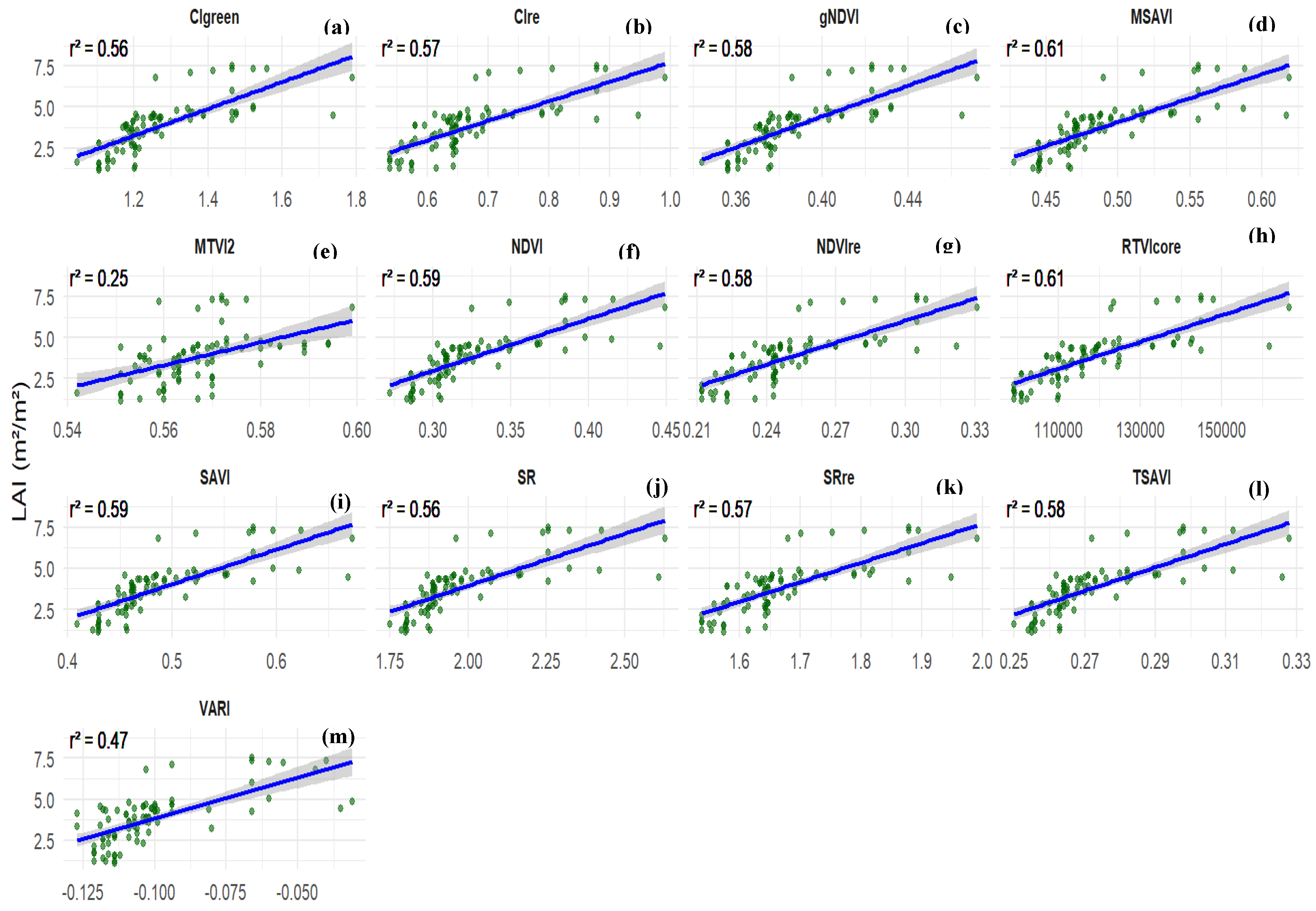
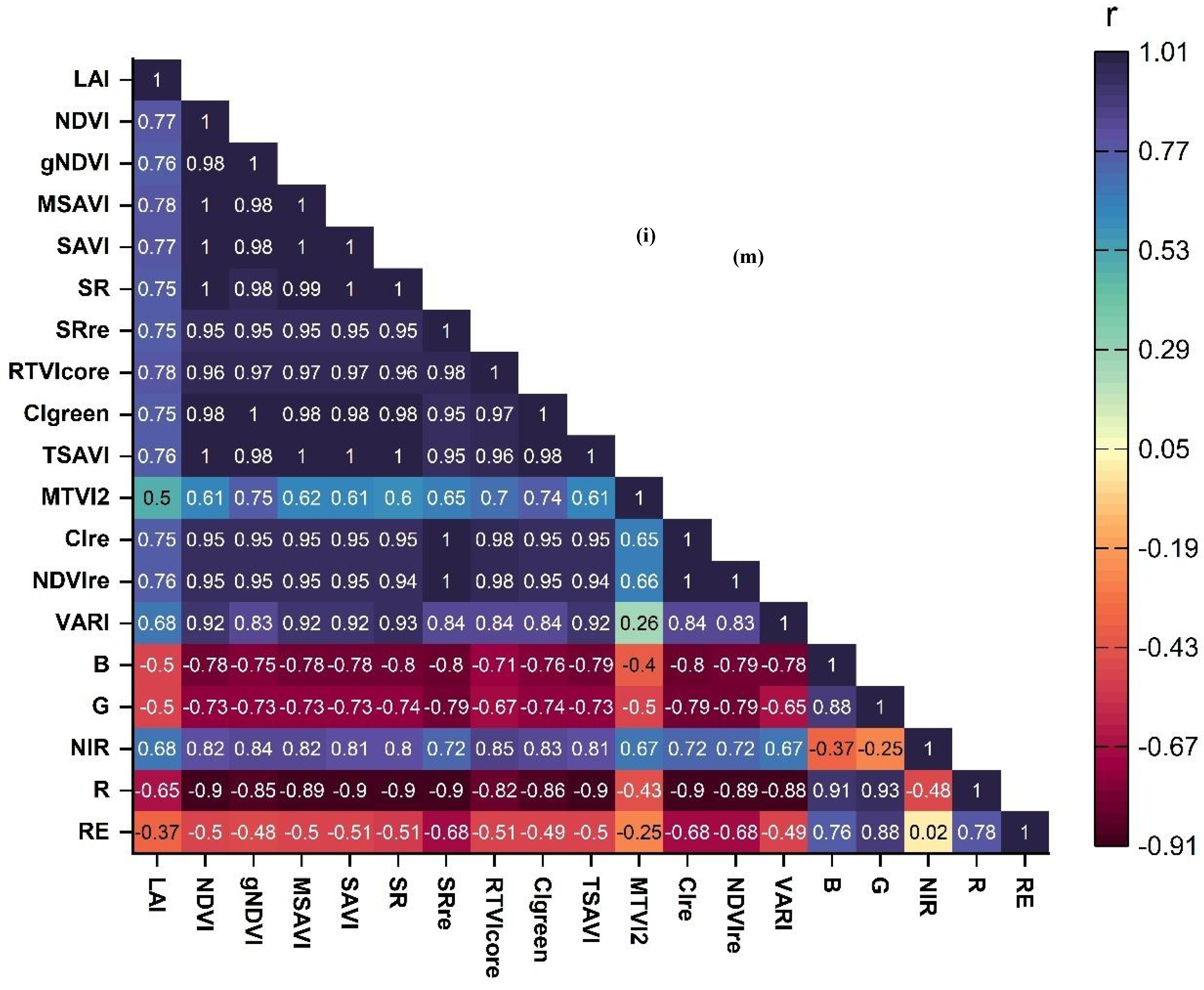
Figure 6.
Pearson’s correlation analysis between LAI, spectral bands, and VIs. All the VIs showed positive relationships with LAI, while all the spectral bands (except NIR) were negatively correlated with LAI.
Figure 6.
Pearson’s correlation analysis between LAI, spectral bands, and VIs. All the VIs showed positive relationships with LAI, while all the spectral bands (except NIR) were negatively correlated with LAI.
Since minimum RMSE values imply the best prediction accuracy, the results showed that the SR and RTVIcore are the best single predictors using the RF algorithm (r2 = 0.84, RMSE = 0.62 m2/m2). Further results demonstrated that the RTVIcore is the best single VI for predicting peanut LAI using the XGBoost (r2 = 0.88, RMSE = 0.52 m2/m2); and the RTVIcore and MSAVI are the top predictors using the PLSR (r2 = 0.61, RMSE = 0.96 m2/m2). Our results suggest that the RTVIcore (using the XGBoost model) plays a significant role in the estimation of peanut LAI. These findings are consistent with those reported by Kross et al. (2015), who identified RTVIcore as the most effective index for estimating LAI and total biomass. Overall, the results indicate that all the VIs derived from high-resolution PlanetScope imagery can estimate peanut LAI with reasonable accuracy, as shown by statistically significant correlations at the 0.05 confidence level. Among the evaluated algorithms, XGBoost demonstrated superior performance compared to RF and PLSR in predicting LAI using single predictor variables (see Figure 7, Figure 8 and Figure 9).
Figure 7.
Relationships between measured and estimated peanut LAI based on vegetation indices and random forest model.
Figure 7.
Relationships between measured and estimated peanut LAI based on vegetation indices and random forest model.
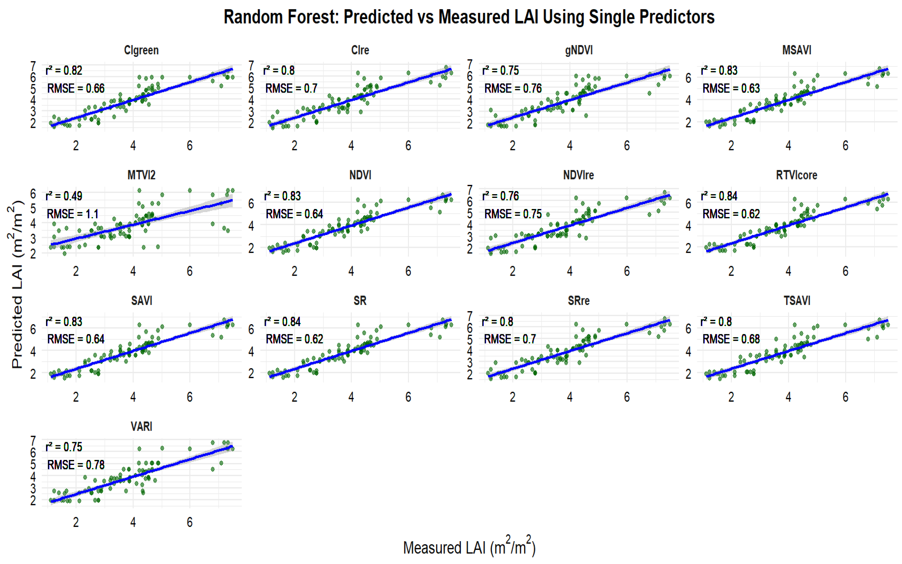
Figure 8.
Relationships between measured and estimated peanut LAI based on vegetation indices and XGBoost model.
Figure 8.
Relationships between measured and estimated peanut LAI based on vegetation indices and XGBoost model.
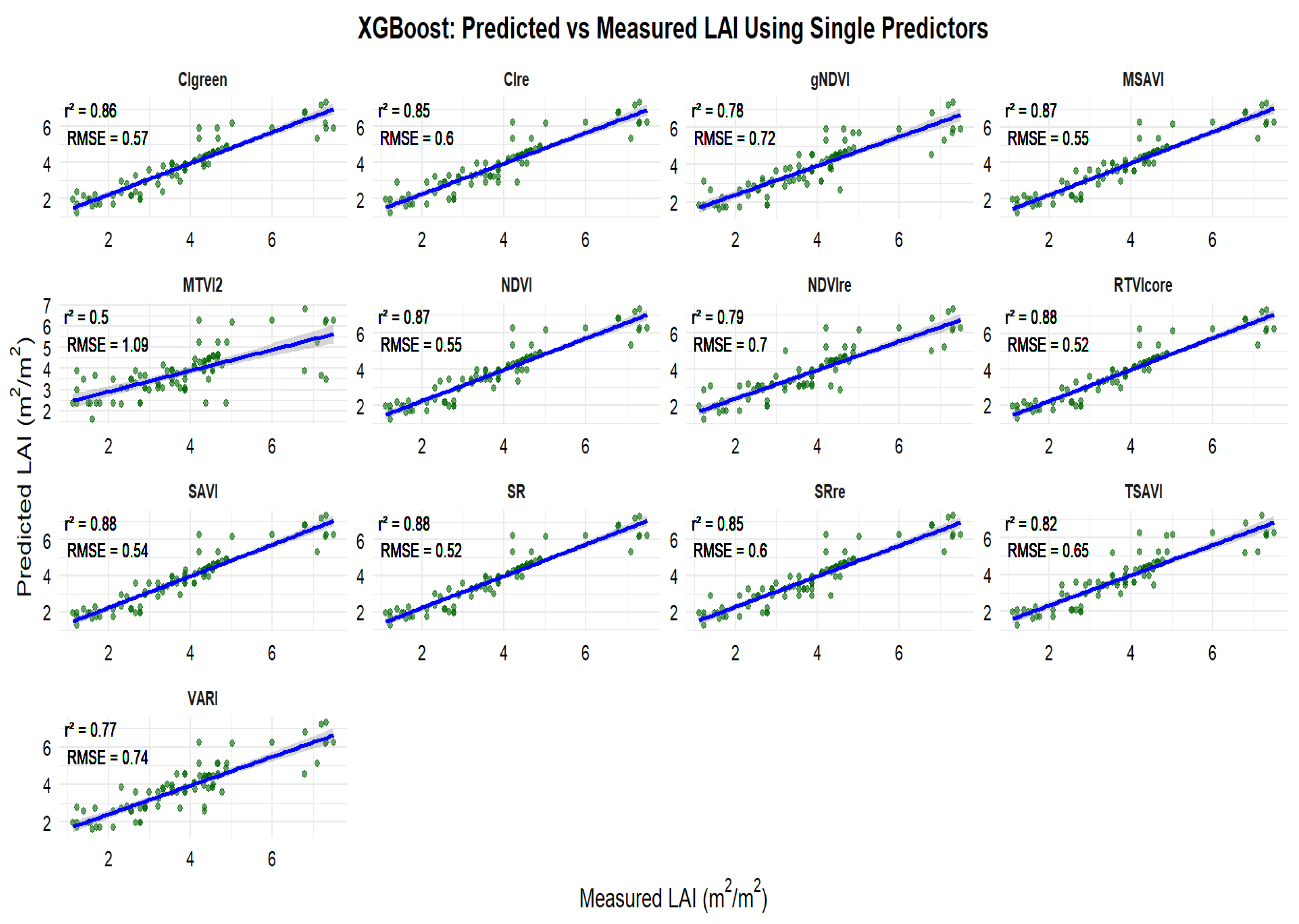
Figure 9.
Relationships between measured and estimated peanut LAI based on vegetation indices and PLSR model.
Figure 9.
Relationships between measured and estimated peanut LAI based on vegetation indices and PLSR model.
3.4. Selection of Important Variables for Peanut LAI Estimation
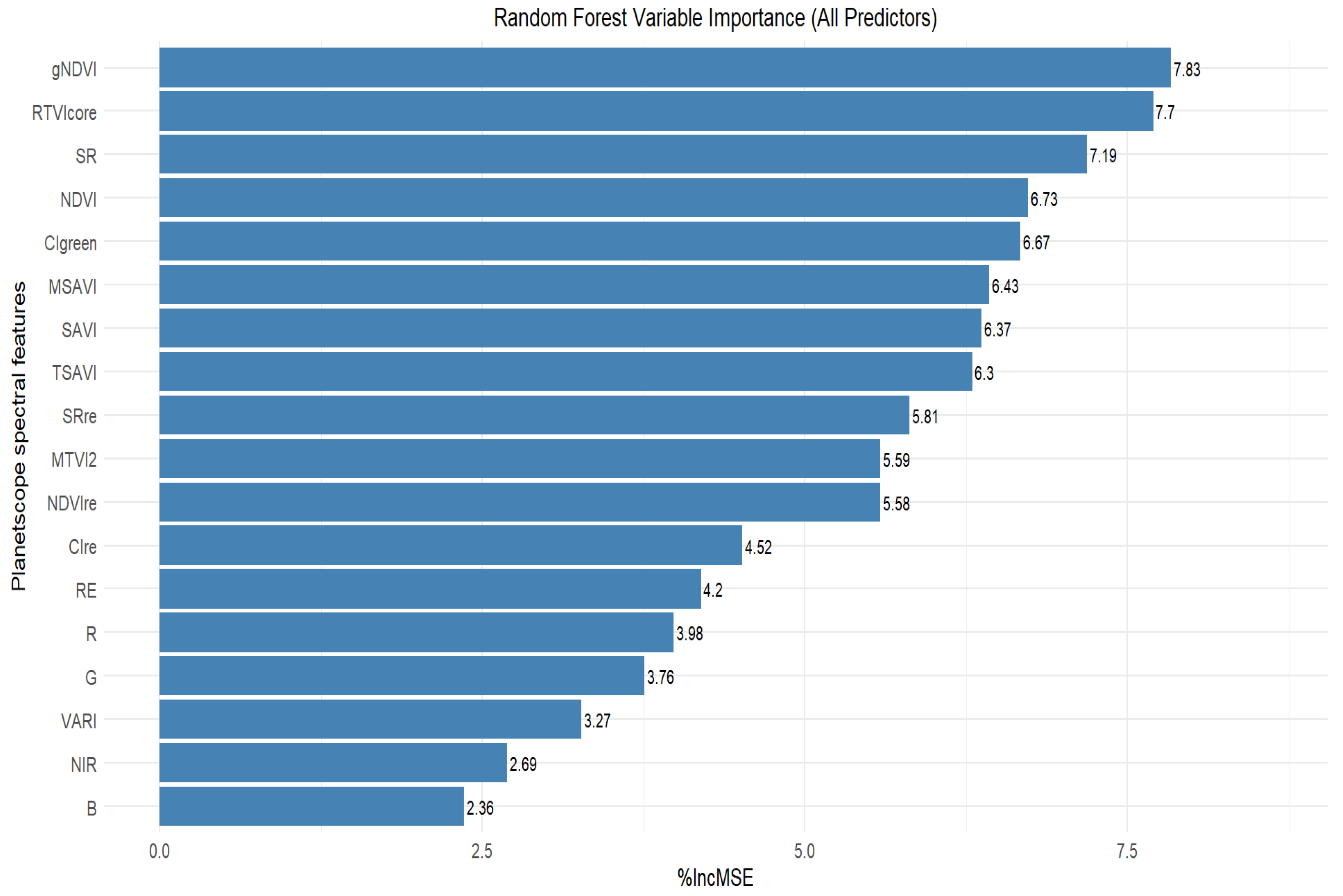
Variable screening plays a critical role in identifying the most influential input variables, thereby enhancing model predictive accuracy. This step is important, as evidenced in the literature, which underscores that input variables differ in their relevance and contribution to model performance, making the assessment of individual variable importance a fundamental aspect of the modeling process (Dube et al., 2017). In this study, eighteen predictor variables (Table 1) were evaluated for their relevant importance for LAI estimation. The results, as shown in Figure 10, revealed that for the PlanetScope spectral reflectances, the red-edge band was the most important predictor, followed by the red band, with %IncMSE values of 4.2 and 3.98, respectively, while the blue band was relatively the worst predictor with a %IncMSE of 2.36. Consistent with the findings of this study, Farmonov et al. (2023) reported that the red-edge band 7 (from PlanetScope data) was the most influential spectral band for estimating wheat yield using the RF algorithm. Similarly, Kganyago et al. (2021) demonstrated that the red-edge bands of Sentinel-2, particularly band 5 (705 nm), contributed most significantly to the performance of the RF algorithm for estimating LAI of multiple crops (i.e., maize, beans, and peanuts), which is similar to our results. Reflectance in the red-edge spectral region is highly sensitive to vegetation conditions and has been recognized as a valuable source of information for agricultural monitoring (Sun et al., 2020).
To enhance the interpretability of our results, the spectral features with relative importance values using the RF algorithm, < 6.4 and > 6.4 are considered as exhibiting low and high predictive power, respectively. For RF modeling, we chose spectral features with high predictive power (i.e., %IncMSE values > 6.4). Primarily, the results (Figure 10) showed the varied impact of VIs on the algorithm accuracy for the RF. Among the VIs, gNDVI was by far the most critical explanatory variable, followed by RTVIcore, with %IncMSE values of 7.83 and 7.7, respectively, while the VARI was the least important index (%IncMSE = 3.27). Zhu et al. (2017) demonstrated that VIs derived from the red-edge band—specifically SRre and NDVIre – using WorldView-2 imagery provided superior model accuracy for LAI estimation when employing the RF algorithm. However, in the present study, the red-edge-based index (RTVIcore) derived from PlanetScope imagery was ranked as the second most important variable (after non-red-edge gNDVI) for estimating peanut LAI using the RF.
Figure 10.
Feature Importance plot generated by the RF algorithm from PlanetScope spectral data using the function importance() in the randomForest package. Higher %IncMSE values imply more impact on LAI estimation. The full names of spectral features (spectral bands and VIs) are presented in Table 1. RE, Red-edge; SR, Simple ratio; NDVI, Normalized Difference Vegetation Index; etc.
The results shown in Figure 11 revealed that for the spectral bands, the green band has the highest contribution to XGBoost model performance, followed by the blue band, with Gain% values of 3.9% and 1.8%, respectively, while the red band has relatively low importance with Gain% of 0.1%. Liu et al. (2021) reported that the NIR band (derived from multispectral unmanned aerial vehicle (UAV) data) yielded the highest accuracy in simulating rice LAI using both RF (R² = 0.73, RMSE = 0.98) and XGBoost (R² = 0.77, RMSE = 0.88) algorithms. In contrast, our findings indicate that the green band using the XGBoost demonstrated greater performance for peanut LAI estimation. For ease of interpretation of results in this study, the spectral features with feature importance values using the XGBoost, < 4% and > 4% are regarded as having low and high predictive power, respectively. For XGBoost modeling in this study, we chose spectral features with high predictive power (i.e., Gain% values > 4%). Generally, the results (Figure 11) showed that, using the XGBoost model, the RTVIcore has the greatest influence on the model accuracy (i.e., Gain% = 40.4%), followed by CIgreen and MSAVI, with Gain% values of 19% and 12.7%, respectively, while SR showed poor influence on XGBoost performance (i.e., Gain% = 0.1%).
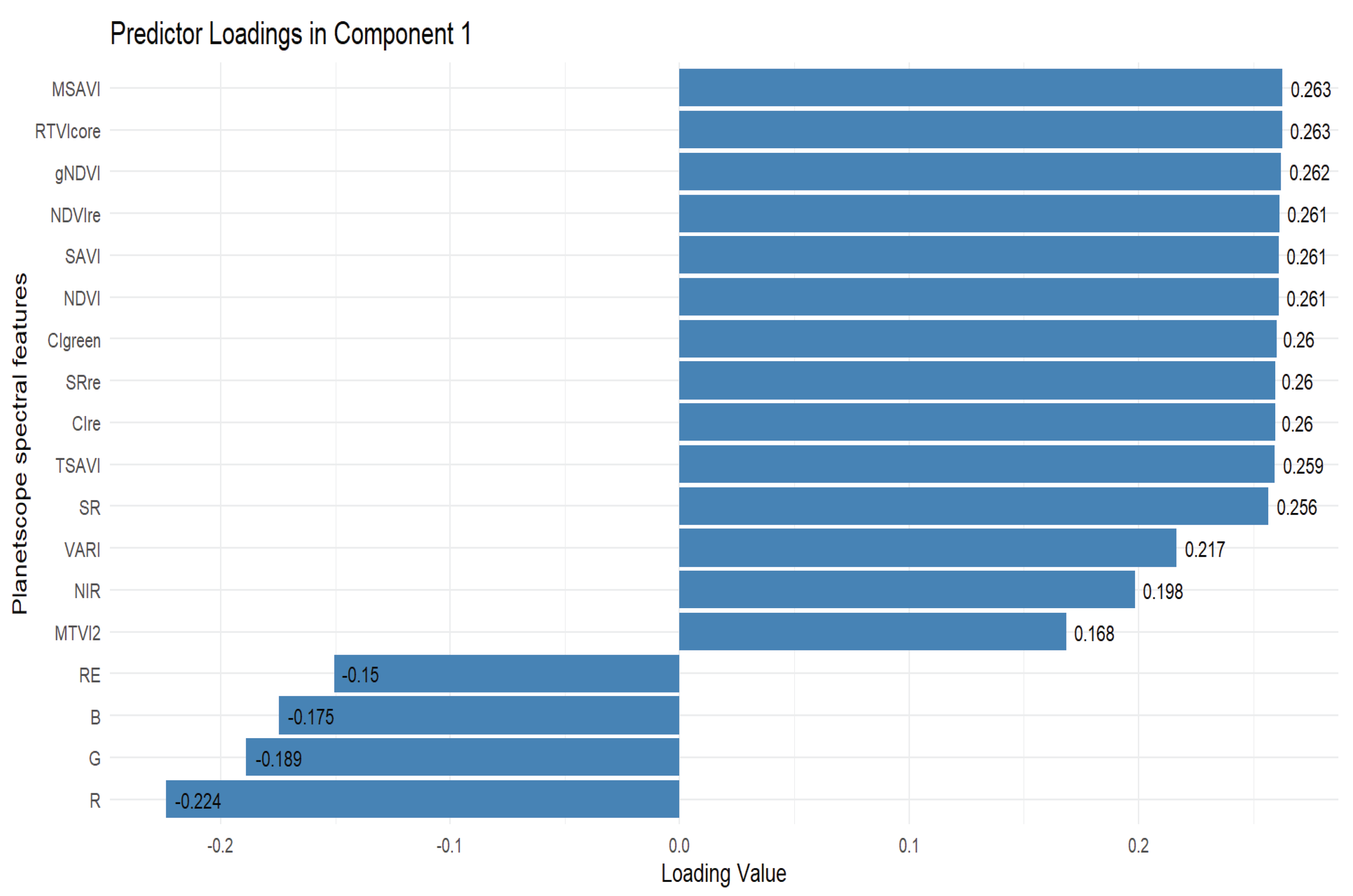
For the PLSR, various PLS components were evaluated, and Component 1, identified as the most influential based on its VIP score of 0.58 (Figure 12) was selected for estimating LAI using the PLSR algorithm. The important spectral features that contributed to Comp 1’s influence on model performance indicate that the most important VIs were MSAVI and RTVIcore (loading values = 0.263), followed by gNDVI (loading value = 0.262), while the worst contributor was MTVI2 with the lowest loading value of 0.168 (Figure 13). All the spectral bands (red-edge, blue, green, and red), except the NIR band (loading value = 0.198) showed negative influence on model performance. This suggests that the inclusion of red-edge, blue, green, and red bands could reduce the accuracy of the PLSR algorithm for estimating peanut LAI.
Figure 11.
Feature Importance plot generated by the XGBoost algorithm from PlanetScope spectral data, using the xgb.importance() function in xgboost package. Higher Gain (%) values represent more impact on model performance accuracy. Spectral features with 0% predictive power were excluded from the plot. The full names of spectral features (spectral bands and vegetation indices) are presented in Table 1. RE, Red-edge; SR, Simple ratio; etc.
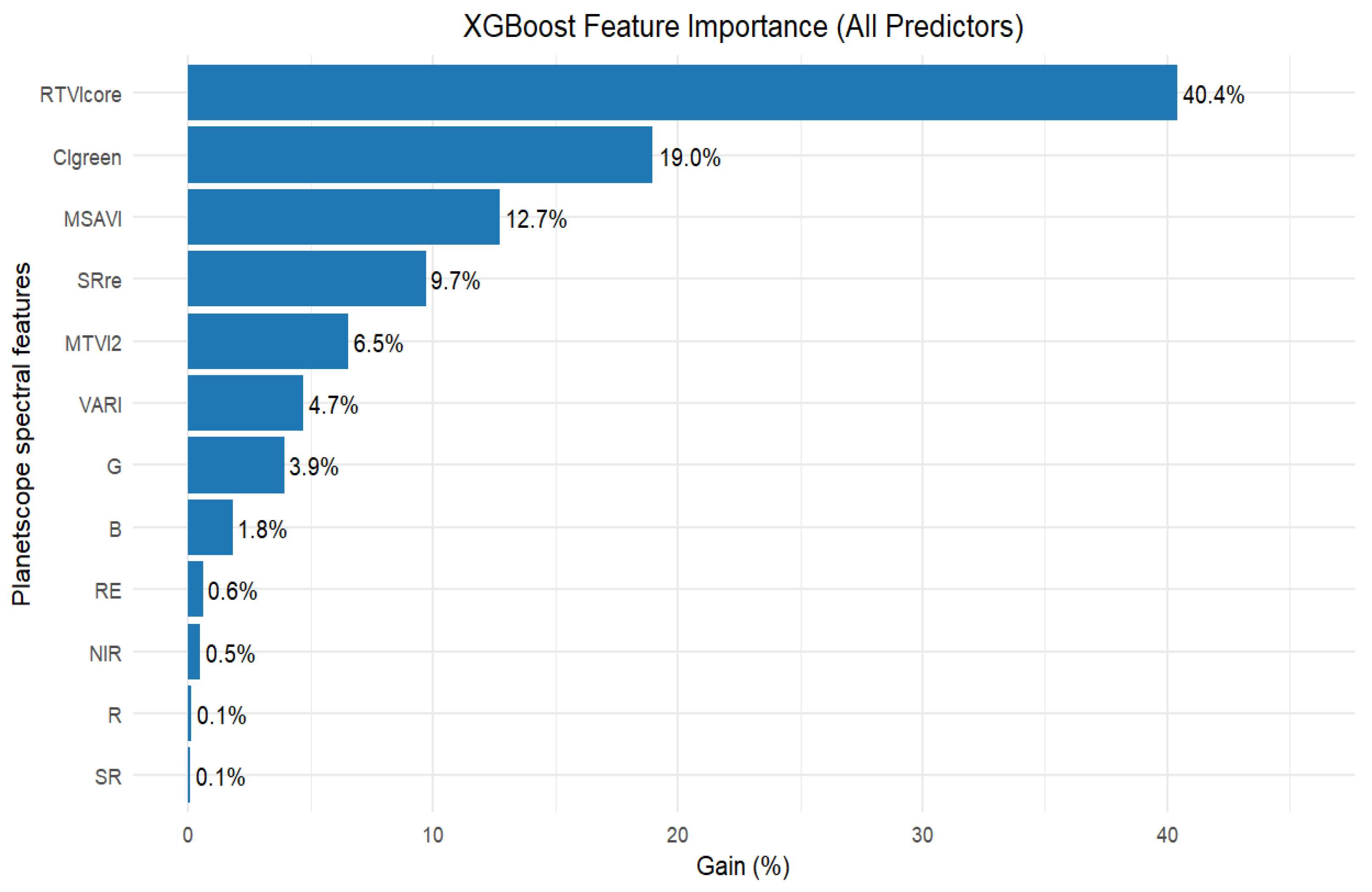
Figure 12.
VIP scores of different components for estimating peanut LAI using the PLSR Variable importance in projection (VIP) function. Higher VIP score values are better indicators of how much each predictor influences LAI estimation. In this study, we selected predictors in PLS Comp 1.
Figure 12.
VIP scores of different components for estimating peanut LAI using the PLSR Variable importance in projection (VIP) function. Higher VIP score values are better indicators of how much each predictor influences LAI estimation. In this study, we selected predictors in PLS Comp 1.
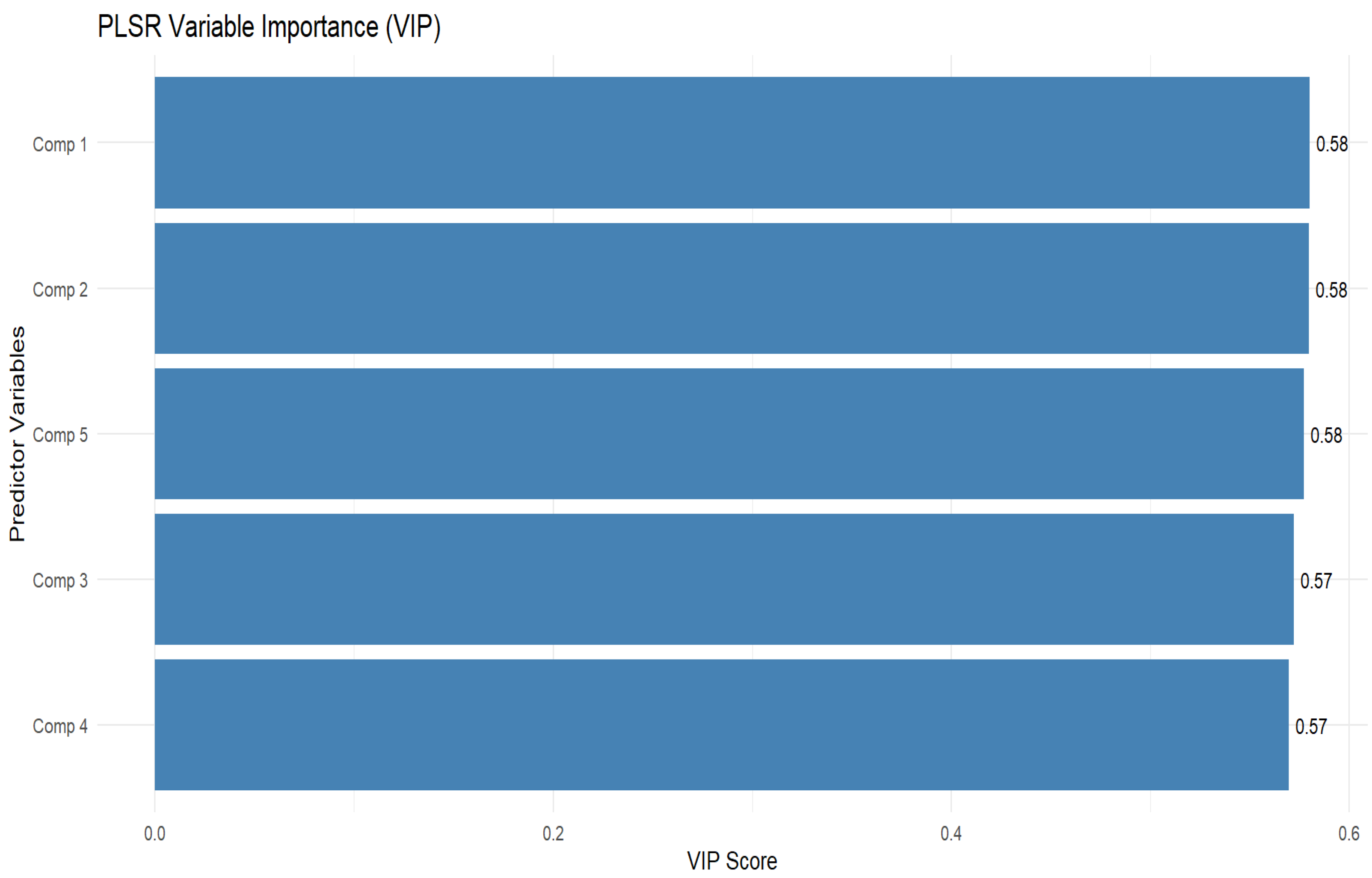
Figure 13.
PLSR Variable importance in projection (VIP) function. Higher loading values indicate a stronger contribution of a variable to PLS Comp 1. In this study, six VIs with the highest loading values greater than 0.26 in Comp 1 were selected for PLSR modeling.
Figure 13.
PLSR Variable importance in projection (VIP) function. Higher loading values indicate a stronger contribution of a variable to PLS Comp 1. In this study, six VIs with the highest loading values greater than 0.26 in Comp 1 were selected for PLSR modeling.
3.5. Estimation of Peanut LAI Based on Machine Learning and Statistical Algorithms Using Important Predictor Variables
From the feature importance plots (Figure 10, Figure 11 and Figure 13), different data combinations of variables were used to train the RF, XGBoost, and PLSR algorithms, including the top three spectral bands, all spectral bands, the top six VIs, and all spectral features combined (i.e., spectral bands and VIs) (see Table 3).
We analyzed the spectral bands (top 3 bands based on variable importance and all five spectral bands) as input variables in the three algorithms. The top three spectral bands based on feature importance for each algorithm (Figure 10, 11 and 13) are as follows: (red-edge, red, green), (green, blue, red-edge), and (red-edge, NIR, blue) for the RF, XGBoost, and PLSR, respectively. The five spectral bands used as predictors in all the algorithms include: red-edge, red, green, NIR, and blue. The results showed that incorporating all the spectral bands in the three algorithms as predictor variables led to improved LAI estimation accuracy compared to using only the top three bands based on feature importance (see Table 3).
Meanwhile, assessing based on the values of %IncMSE > 6.4, Gain% > 4%, and loading value ≥ 0.261 as shown in Figure 10, 11 and 13, respectively, we selected the top six VIs (gNDVI, RTVIcore, SR, NDVI, CIgreen, MSAVI), (RTVIcore, CIgreen, MSAVI, SRre, MTVI2, VARI), and (MSAVI, RTVIcore, gNDVI, NDVIre, SAVI, NDVI) as the best predictors for the estimation of peanut LAI using the RF, XGBoost, and PLSR, respectively. Our results demonstrate that VIs derived from spectral bands provide superior model accuracy in estimating LAI compared to the use of spectral bands alone (see Table 3). These findings are consistent with the results of Tunca et al. (2024), who reported that using VIs computed from multiple spectral bands as input features were more effective for estimating sorghum LAI than using individual spectral bands alone. Similar findings were reported by Dube et al. (2017), who demonstrated that integrating VIs with traditional RGBNIR bands from RapidEye imagery improved LAI estimation accuracy by approximately 20% compared to using red, green, blue, and near-infrared (RGBNIR) bands or RGBNIR indices as independent predictor variables. In contrast to our findings, Chatterjee et al. (2025) found that reflectance-based models outperformed vegetation index-based models, particularly during the mid to late vegetative stage of corn growth (by 5–15%) and at the silking stage (by 25%). According to Chatterjee et al. (2025), the superior performance of reflectance-based models was primarily attributed to the red-edge and NIR bands, due to their increased sensitivity to higher LAI values.
We also tested the influence of using all the spectral features (spectral bands and VIs) on model performance accuracy. The findings underscore the critical role of feature selection in model calibration, as the results showed that incorporating all the spectral bands and VIs did not enhance the performance of the RF, XGBoost, and PLSR algorithms in estimating peanut LAI (see Table 3). For instance, in the case of the RF, incorporating all spectral features led to a reduction in model accuracy, with an RRMSE increase of 2.05% compared to using only the top six VIs. Similarly, for the XGBoost, the use of all spectral features resulted in a slight RRMSE increase of 0.15%. The most significant reduction in accuracy was observed in the PLSR algorithm, where including all spectral features increased the RRMSE by 3.51% compared to using the top six VIs alone. These results are consistent with the results of Shen et al. (2024), who demonstrated that using all the features in an algorithm does not necessarily improve predictive accuracy, and may, in fact, result in reduced accuracy.
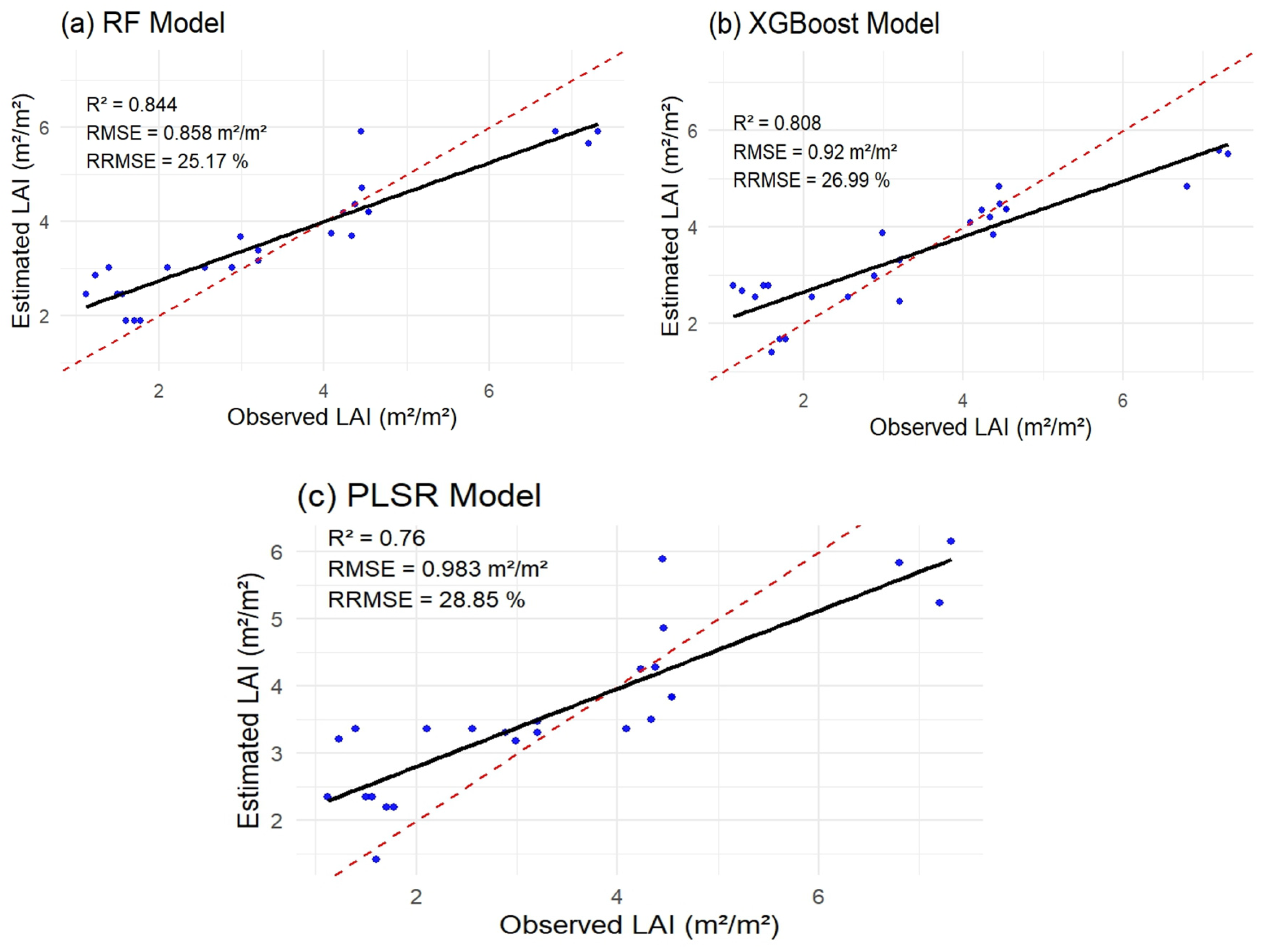
The LAI estimation results (Figure 14a–c) indicate that the RF achieved the highest predictive performance, with an RRMSE of 25.17%, RMSE of 0.858 m²/m², and explaining 84.4% of LAI variability (Figure 14a). This was followed by the XGBoost algorithm, which yielded an RRMSE of 26.99%, an RMSE of 0.92 m²/m², and an R² of 0.808 (Figure 14b). The relatively similar RRMSE values of the RF and XGBoost suggest that both algorithms exhibited comparable predictive capabilities in estimating peanut LAI. This is expected, as both methods are ensemble models based on decision trees (Li et al., 2023), sharing fundamental characteristics such as the ability to reduce overfitting through ensemble strategies—bagging and boosting for RF and XGBoost, respectively. Moreover, ensemble tree-based models are inherently better suited to capturing non-linear relationships between VIs and LAI (Intarat et al., 2025). In contrast, further results showed that the PLSR algorithm exhibited the least predictive accuracy, with an RRMSE of 28.85%, and an RMSE of 0.983 m²/m², and explained 76% of variability in LAI (Figure 14c). The findings of Intarat et al., (2025) demonstrated that PLSR performed statistically worse in estimating rice LAI, which is consistent with our results. The relatively lower performance of the PLSR model in estimating LAI can be attributed to its limitation of dealing with non-linear relationships between VIs and LAI (Rivera-Caicedo et al., 2017; Intarat et al., 2025).
Previous studies have shown the difficulty in using the traditional VIs to estimate crop LAI due to saturation of the VIs and their low sensitivity when medium to high LAI values are present (Nguy-Robertson et al., 2012; Kross et al., 2015). In this study, however, we found the feasibility of estimating peanut LAI using multiple VIs derived from high-resolution PlanetScope data and nonparametric ML and statistical algorithms. Meanwhile, compared to using VI-based parametric regression models (using fitting functions, e.g., linear, power, exponential, etc.), nonparametric ML models are well-known for their ability to minimize multicollinearity issues (Martínez-Muñoz & Suárez, 2010; Garg & Tai, 2013). While RF and XGBoost algorithms both exhibited strong results compared to the PLSR in estimating peanut LAI, the RF algorithm demonstrated a slightly higher predictive accuracy, consistent with the findings reported in previous studies (Kganyago et al., 2021). The superior performance of the RF algorithm in predicting LAI in this study may be attributed to its robustness to noise and potential to capture nonlinear interactions among input features. Kganyago et al. (2021) employed RF, sparse Partial Least Squares (sPLS), and Gradient Boosting Machine (GBM) to estimate LAI, leaf chlorophyll content (LCab), and canopy chlorophyll content (CCC) for maize, beans, and peanuts. Their results indicated that RF outperformed both sPLS and GBM across all three crops’ parameters, which is similar to our results. Recent studies have also demonstrated the superiority of RF methods in estimating LAI in various crops, such as in winter wheat crops (Tang et al., 2022), paddy rice (Wang et al., 2018b), maize (Gao et al., 2024), winter rapeseed (Zhang et al., 2023), and potato (Yu et al., 2023). Therefore, integrating important VIs into the ML models, such as RF, can help mitigate the saturation effects commonly observed by using only single VIs.
Figure 14.
Scatterplots for Leaf Area Index (LAI, m2/m2) showing the performance of: (a) random forest (RF), (b) eXtreme gradient boosting (XGBoost), and (c) partial least squares regression (PLSR) with Planetscope data. The red dashed line represents the 1:1 line, indicating perfect agreement between observed and estimated LAI values. The solid black line is the regression (trend) line fitted to the data points.
3.6. Generation of Peanut LAI Prediction Maps Based Different Models
The top six VIs, identified based on their relative feature importance in Figure 10, Figure 11 and Figure 13 for the RF, XGBoost, and PLSR algorithms respectively, were selected to generate the final LAI prediction maps. This decision was based on validation results (presented in Table 3), which demonstrated that the top six VIs yielded superior predictive performance for estimating peanut LAI compared to algorithms incorporating the top three spectral bands (or all spectral bands) and the combination of spectral features (bands and VIs). In the final LAI prediction maps as shown in Figure 15. The low and high LAI regions are depicted in red and dark blue hues, respectively, which showed distinct variations of LAI in the field.
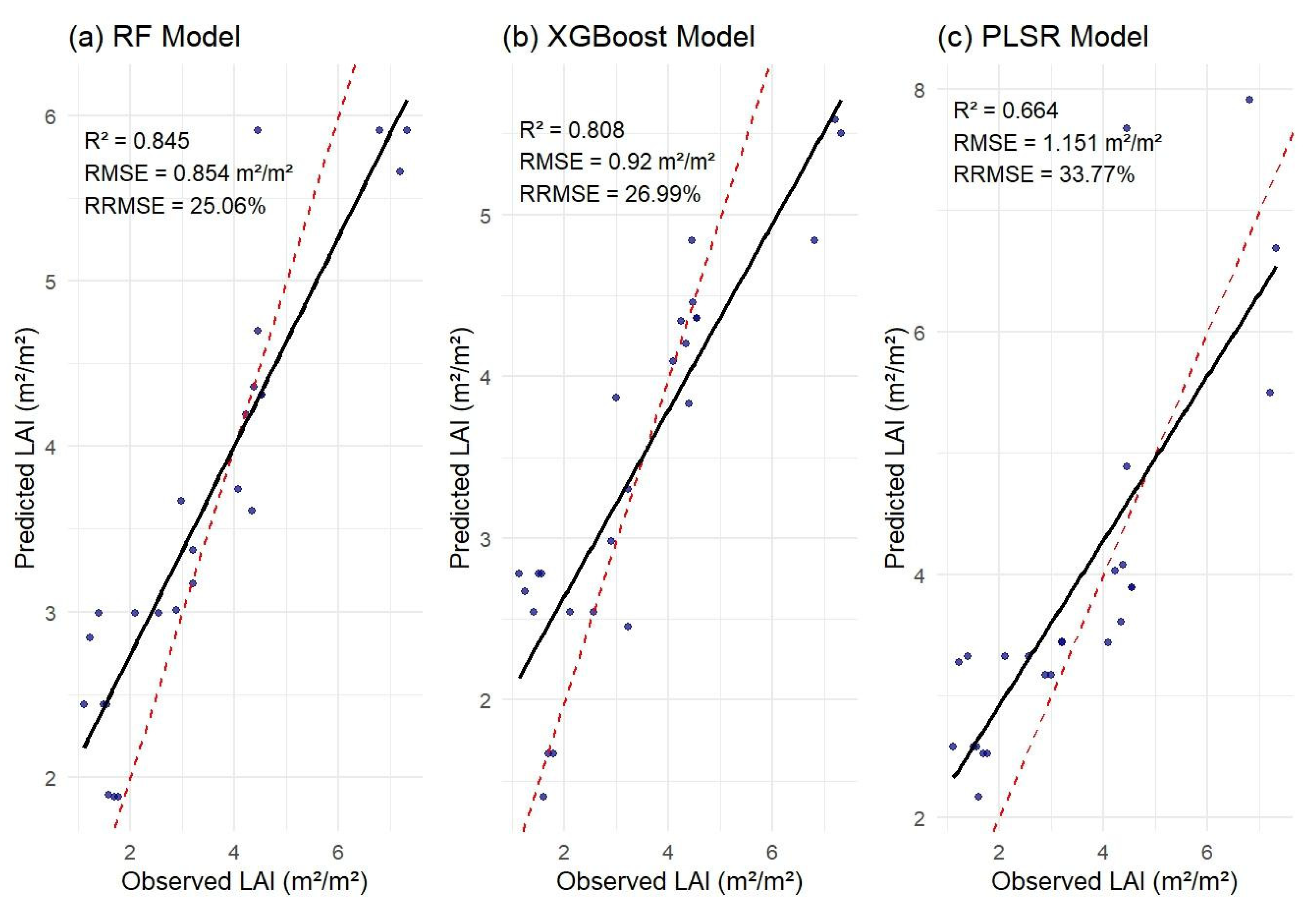
The RF, XGBoost, and PLSR algorithms were applied to PlanetScope images to characterize the spatial variability of LAI within the peanut field. The RF-based prediction map recorded a mean LAI value of 5.18 m²/m² (Figure 15a). Inspection of the RF map demonstrated that higher LAI values were predominantly clustered in the south-western and north-central regions of the field, while lower LAI values were predicted over the northern areas. The RF algorithm demonstrated robust performance, effectively capturing finer-scale variability of LAI in the field (Figure 15a). The XGBoost-based prediction map showed a similar spatial pattern as the RF, with a mean LAI value of 5.02 m²/m² (Figure 15b). In contrast, the PLSR-based map recorded the lowest average LAI value of 3.53 m²/m² (Figure 15c). In addition, we observed that the PLSR-based prediction map shows increased spatial heterogeneity, suggesting that the algorithm struggled to accurately capture the spatial variability of LAI using the PlanetScope data. However, the algorithm exhibited a consistent bias, tending to underestimate LAI in regions with higher observed LAI values (Figure 15c). Again, the comparable and superior performance of RF and XGBoost algorithms in mapping peanut LAI in this study could be linked to the capability of these ensemble-based models to capture nonlinear relationships between LAI and PlanetScope spectral features, compared to PLSR, which is inherently limited in its ability to capture nonlinear interactions, thereby reducing its predictive performance. Inspection of the PLSR prediction map (Figure 15c) showed a broad spatial distribution of lower LAI values (i.e., < 3 m²/m²), particularly concentrated in the northern, north-central, and south-eastern regions of the field, while the lowest LAI values predicted by the RF (Figure 15a) and XGBoost (Figure 15b) algorithms in the same regions are generally above 3 m²/m². The findings of Rivera-Caicedo et al. (2017) demonstrated that the PLSR algorithm tends to perform better in predicting lower values compared to other models, which is consistent with our results. From the prediction rasters, we extracted the predicted LAI estimates at each validation sampling point and compared the estimates with the measured LAI values. The performance evaluation indicated that the RF algorithm achieved the highest accuracy (R² = 0.845, RMSE = 0.854 m²/m², RRMSE = 25.06%), followed by the XGBoost (R² = 0.808, RMSE = 0.92 m²/m², RRMSE = 26.99%), while the PLSR exhibited the lowest performance (R² = 0.664, RMSE = 1.151 m²/m², RRMSE = 33.77%) (Figure 16).
Figure 15.
Peanut LAI prediction maps based on the three algorithms: (a) RF, (b) XGBoost, and (c) PLSR. LAI prediction maps were generated using the top six VIs: (gNDVI, RTVIcore, SR, NDVI, CIgreen, MSAVI), (RTVIcore, CIgreen, MSAVI, SRre, MTVI2, VARI), and (MSAVI, RTVIcore, gNDVI, NDVIre, SAVI, NDVI) for RF, XGBoost, and PLSR, respectively.
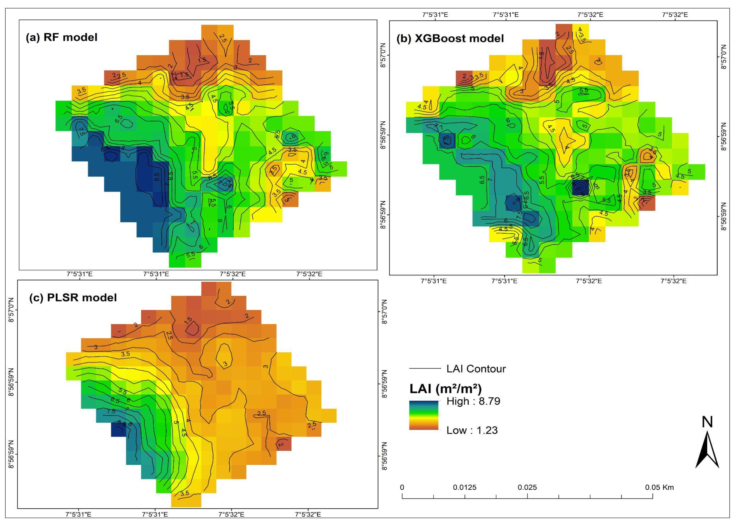
Figure 16.
Relationships between observed LAI (validation data) and LAI extracted from the prediction maps based on the three tested algorithms: (a) RF, (b) XGBoost, and (c) PLSR. The red dashed line represents the 1:1 line, indicating perfect agreement between observed and predicted LAI values. The solid black line is the regression (trend) line fitted to the data points.
4. Conclusions and Recommendations
This study evaluated the performance of Random Forest (RF), eXtreme Gradient Boosting (XGBoost), and Partial Least Squares Regression (PLSR) algorithms in estimating peanut LAI using spectral features derived from high spatial-temporal resolution PlanetScope data. Thirteen VIs were assessed for the estimation of peanut LAI. Overall, most VIs exhibited strong positive linear relationships with LAI (r > 0.75), but showed some saturation when LAI reached 3 m²/m². The thirteen VIs assessed individually revealed that their performance varied in predicting peanut LAI using RF, XGBoost and PLSR models. The results indicated that the SR and RTVIcore had the highest LAI estimation accuracy in the RF model, RTVIcore was the best index in the XGBoost model, and RTVIcore and MSAVI performed superior to other VIs in the PLSR model.
Moreover, the spectral features (bands and VIs) that had the highest influence on the model accuracy were identified using the RF, XGBoost, and PLSR feature importance metrics. The gNDVI was identified as the most important predictor of peanut LAI using RF model. The RTVIcore had the highest influence on XGBoost model performance accuracy. For the PLSR algorithm, the MSAVI and RTVIcore were the important predictors of LAI estimates. Further, our results demonstrated that spectral indices derived from PlanetScope bands exhibited greater predictive accuracy compared to accuracy using spectral bands in the estimation of peanut LAI. Meanwhile, the integration of spectral bands and VIs identified through variable importance analysis, was evaluated for LAI estimation, and the results showed that combining bands and VIs led to a reduction in prediction accuracy for LAI estimates, highlighting the significance of selecting important predictor variables to guarantee the best accuracy. Overall, our results demonstrated that the RF model provides the most robust predictive performance for peanut LAI using PlanetScope data, therefore making it a strong candidate for operational applications.
However, certain limitations should be admitted in this study. First, the in situ LAI dataset was relatively small, which may limit the robustness of model calibration and validation. Additionally, field measurements were conducted only at the maturity stage of the peanut crop, limiting the evaluation of model performance across different growth stages. Future research will aim to collect a larger number of in situ samples to enhance the representativeness and reliability of model training. Moreover, field experiments will be extended to multiple phenological stages throughout the growing season to better assess the models’ ability to estimate peanut LAI across various developmental phases. Finally, future studies will focus on evaluating the transferability of peanut LAI prediction models to assess their performance across diverse geographic regions, crop types, and environmental conditions.
CRediT authorship contribution statement
M. Ekwe: Field data collection, conceptualization, methodology, software, validation, formal analysis, resources, Writing - original draft, editing. H. Fernando: Formal analysis, methodology, Writing - review & editing. G. James: Writing - review & editing. O. Adeluyi: Methodology, Formal analysis, Writing - review & editing. J. Verrelst: Methodology, software, Writing - review & editing. A. Kross: Supervision, Writing - review & editing.
Funding
This research received no external funding to report.
Data Availability Statement
The original contributions of this study are presented within the article. For additional information, researchers are encouraged to contact the corresponding author. The in situ peanut LAI data and raw R scripts used in the analysis are available upon request.
Acknowledgments
The authors acknowledge the School of Agriculture, Food and Wine, the University of Adelaide, for the design and development of the VitiCanopy App deployed freely in this project. The authors also gratefully acknowledge Planet Labs, Inc. for providing us with the PlanetScope data used in this study under the Education and Research Program.
Ethical statement
We hereby declare that:. -This work is not under consideration for publication elsewhere and will not be submitted to another journal before a final decision is made. -The content of this manuscript is entirely original, and all sources of information or previously published work have been appropriately cited or quoted.
Declaration of competing interest
The authors declare no conflict of interest.
References
- Abd El-Ghany, N. M., Abd El-Aziz, S. E., & Marei, S. S. (2020). A review: Application of remote sensing as a promising strategy for insect pests and diseases management. Environmental Science and Pollution Research, 27(27), 33503–33515. [CrossRef]
- Ajeigbe H.A., Waliyar F., Echekwu C.A, Ayuba K., Motagi B.N., Eniayeju D. and Inuwa A. (2015). A Farmer’s Guide to Groundnut Production in Nigeria. Patancheru 502 324, Telangana, India: International Crops Research Institute for the Semi-Arid Tropics. 36 pp.
- Ali, A. M., Abouelghar, M., Belal, A. A., Saleh, N., Yones, M., Selim, A. I., Amin, M. E. S., Elwesemy, A., Kucher, D. E., Maginan, S., & Savin, I. (2022). Crop Yield Prediction Using Multi Sensors Remote Sensing (Review Article). The Egyptian Journal of Remote Sensing and Space Science, 25(3), 711–716. [CrossRef]
- Amankulova, K., Farmonov, N., Akramova, P., Tursunov, I., & Mucsi, L. (2023). Comparison of PlanetScope, Sentinel-2, and landsat 8 data in soybean yield estimation within-field variability with random forest regression. Heliyon, 9(6), e17432. [CrossRef]
- Anees, S. A., Mehmood, K., Khan, W. R., Sajjad, M., Alahmadi, T. A., Alharbi, S. A., & Luo, M. (2024). Integration of machine learning and remote sensing for above ground biomass estimation through Landsat-9 and field data in temperate forests of the Himalayan region. Ecological Informatics, 82, 102732. [CrossRef]
- Bahrami, H., Homayouni, S., McNairn, H., Hosseini, M., & Mahdianpari, M. (2022). Regional Crop Characterization Using Multi-Temporal Optical and Synthetic Aperture Radar Earth Observations Data. Canadian Journal of Remote Sensing, 48(2), 258–277. [CrossRef]
- Barboza, T. O. C., Souza, J. B. C., Ferraz, M. A. J., De Almeida, S. L. H., Pilon, C., Vellidis, G., Da Silva, R. P., & Dos Santos, A. F. (2025). Application of artificial intelligence for identification of peanut maturity using climatic variables and vegetation indices. Precision Agriculture, 26(3), 43. [CrossRef]
- Baret, F., Guyot, G., & Major, D. J. (1989). TSAVI: A Vegetation Index Which Minimizes Soil Brightness Effects On LAI And APAR Estimation. 12th Canadian Symposium on Remote Sensing Geoscience and Remote Sensing Symposium, 3, 1355–1358. [CrossRef]
- Beckschäfer, P., Fehrmann, L., Harrison, R., Xu, J., & Kleinn, C. (2014). Mapping Leaf Area Index in subtropical upland ecosystems using RapidEye imagery and the randomForest algorithm. iForest - Biogeosciences and Forestry, 7(1), 1–11. [CrossRef]
- Behera, S. K., Srivastava, P., Pathre, U. V., & Tuli, R. (2010). An indirect method of estimating leaf area index in Jatropha curcas L. using LAI-2000 Plant Canopy Analyzer. Agricultural and Forest Meteorology, 150(2), 307–311. [CrossRef]
- Belaqziz, S., Khabba, S., Kharrou, M. H., Bouras, E. H., Er-Raki, S., & Chehbouni, A. (2021). Optimizing the Sowing Date to Improve Water Management and Wheat Yield in a Large Irrigation Scheme, through a Remote Sensing and an Evolution Strategy-Based Approach. Remote Sensing, 13(18), 3789. [CrossRef]
- Belgiu, M., & Drăguţ, L. (2016). Random forest in remote sensing: A review of applications and future directions. ISPRS Journal of Photogrammetry and Remote Sensing, 114, 24–31. [CrossRef]
- Ben Asher, J., Bar Yosef, B., & Volinsky, R. (2013). Ground-based remote sensing system for irrigation scheduling. Biosystems Engineering, 114(4), 444–453. [CrossRef]
- Beven, K. J., & Kirkby, M. J. (1979). A physically based, variable contributing area model of basin hydrology / Un modèle à base physique de zone d’appel variable de l’hydrologie du bassin versant. Hydrological Sciences Bulletin, 24(1), 43–69. [CrossRef]
- Breiman, L. (2001). Random forests. Machine Learning, 45(1), 5–32. [CrossRef]
- Caballero, G., Pezzola, A., Winschel, C., Casella, A., Sanchez Angonova, P., Orden, L., Berger, K., Verrelst, J., & Delegido, J. (2022). Quantifying Irrigated Winter Wheat LAI in Argentina Using Multiple Sentinel-1 Incidence Angles. Remote Sensing, 14(22), 5867. [CrossRef]
- Caicedo, J. P. R., Verrelst, J., Munoz-Mari, J., Moreno, J., & Camps-Valls, G. (2014). Toward a Semiautomatic Machine Learning Retrieval of Biophysical Parameters. IEEE Journal of Selected Topics in Applied Earth Observations and Remote Sensing, 7(4), 1249–1259. [CrossRef]
- Campos-Taberner, M., García-Haro, F., Confalonieri, R., Martínez, B., Moreno, Á., Sánchez-Ruiz, S., Gilabert, M., Camacho, F., Boschetti, M., & Busetto, L. (2016). Multitemporal Monitoring of Plant Area Index in the Valencia Rice District with PocketLAI. Remote Sensing, 8(3), 202. [CrossRef]
- Casa, R., Varella, H., Buis, S., Guérif, M., De Solan, B., & Baret, F. (2012). Forcing a wheat crop model with LAI data to access agronomic variables: Evaluation of the impact of model and LAI uncertainties and comparison with an empirical approach. European Journal of Agronomy, 37(1), 1–10. [CrossRef]
- Chatterjee, S., Baath, G. S., Sapkota, B. R., Flynn, K. C., & Smith, D. R. (2025). Enhancing LAI estimation using multispectral imagery and machine learning: A comparison between reflectance-based and vegetation indices-based approaches. Computers and Electronics in Agriculture, 230, 109790. [CrossRef]
- Chen, J. M., & Black, T. A. (1992). Defining leaf area index for non--flat leaves. Plant, Cell & Environment, 15(4), 421–429. [CrossRef]
- Chen, T., & Guestrin, C. (2016). XGBoost: A Scalable Tree Boosting System. Proceedings of the 22nd ACM SIGKDD International Conference on Knowledge Discovery and Data Mining, 785–794. [CrossRef]
- Chen, P., Tremblay, N., Wang, J., Vigneaulta, P., (2010). New index for crop canopy fresh biomass estimation. Spectrosc. Spectr. Anal. 30, 512–517 (in Chinese).
- Confalonieri, R., Foi, M., Casa, R., Aquaro, S., Tona, E., Peterle, M., Boldini, A., De Carli, G., Ferrari, A., Finotto, G., Guarneri, T., Manzoni, V., Movedi, E., Nisoli, A., Paleari, L., Radici, I., Suardi, M., Veronesi, D., Bregaglio, S., … Acutis, M. (2013). Development of an app for estimating leaf area index using a smartphone. Trueness and precision determination and comparison with other indirect methods. Computers and Electronics in Agriculture, 96, 67–74. [CrossRef]
- De Bei, R., Fuentes, S., Gilliham, M., Tyerman, S., Edwards, E., Bianchini, N., Smith, J., & Collins, C. (2016). VitiCanopy: A Free Computer App to Estimate Canopy Vigor and Porosity for Grapevine. Sensors, 16(4), 585. [CrossRef]
- De Magalhães, L. P., & Rossi, F. (2024). Use of Indices in RGB and Random Forest Regression to Measure the Leaf Area Index in Maize. Agronomy, 14(4), 750. [CrossRef]
- Din, M., Zheng, W., Rashid, M., Wang, S., & Shi, Z. (2017). Evaluating Hyperspectral Vegetation Indices for Leaf Area Index Estimation of Oryza sativa L. at Diverse Phenological Stages. Frontiers in Plant Science, 8, 820. [CrossRef]
- Du, L., Yang, H., Song, X., Wei, N., Yu, C., Wang, W., & Zhao, Y. (2022). Estimating leaf area index of maize using UAV-based digital imagery and machine learning methods. Scientific Reports, 12(1), 15937. [CrossRef]
- Dube, T., Mutanga, O., Sibanda, M., Shoko, C., & Chemura, A. (2017). Evaluating the influence of the Red Edge band from RapidEye sensor in quantifying leaf area index for hydrological applications specifically focussing on plant canopy interception. Physics and Chemistry of the Earth, Parts A/B/C, 100, 73–80. [CrossRef]
- Ekwe, M. C., Adeluyi, O., Verrelst, J., Kross, A., & Odiji, C. A. (2024). Estimating rainfed groundnut’s leaf area index using Sentinel-2 based on Machine Learning Regression Algorithms and Empirical Models. Precision Agriculture. [CrossRef]
- Ennouri, K., Triki, M. A., & Kallel, A. (2020). Applications of Remote Sensing in Pest Monitoring and Crop Management. In C. Keswani (Ed.), Bioeconomy for Sustainable Development (pp. 65–77). Springer Singapore. [CrossRef]
- Fang, H., Baret, F., Plummer, S., & Schaepman--Strub, G. (2019). An Overview of Global Leaf Area Index (LAI): Methods, Products, Validation, and Applications. Reviews of Geophysics, 57(3), 739–799. [CrossRef]
- Farmonov, N., Amankulova, K., Szatmári, J., Urinov, J., Narmanov, Z., Nosirov, J., & Mucsi, L. (2023). Combining PlanetScope and Sentinel-2 images with environmental data for improved wheat yield estimation. International Journal of Digital Earth, 16(1), 847–867. [CrossRef]
- Fatima, S., Hussain, A., Amir, S. B., Ahmed, S. H., & Aslam, S. M. H. (2023). XGBoost and Random Forest Algorithms: An in Depth Analysis. Pakistan Journal of Scientific Research, 3(1), 26–31. [CrossRef]
- Fu, Y., Yang, G., Feng, H., Song, X., Xu, X., & Wang, J. (2013). Comparative analysis of three regression methods for the winter wheat biomass estimation using hyperspectral measurements. Proceedings of the 2nd International Conference on Computer Science and Electronics Engineering (ICCSEE 2013), China. [CrossRef]
- Francone, C., Pagani, V., Foi, M., Cappelli, G., & Confalonieri, R. (2014). Comparison of leaf area index estimates by ceptometer and PocketLAI smart app in canopies with different structures. Field Crops Research, 155, 38–41. [CrossRef]
- Fu, Y., Yang, G., Song, X., Li, Z., Xu, X., Feng, H., & Zhao, C. (2021). Improved Estimation of Winter Wheat Aboveground Biomass Using Multiscale Textures Extracted from UAV-Based Digital Images and Hyperspectral Feature Analysis. Remote Sensing, 13(4), 581. [CrossRef]
- Gao, X., Yao, Y., Chen, S., Li, Q., Zhang, X., Liu, Z., Zeng, Y., Ma, Y., Zhao, Y., & Li, S. (2024). Improved maize leaf area index inversion combining plant height corrected resampling size and random forest model using UAV images at fine scale. European Journal of Agronomy, 161, 127360. [CrossRef]
- Garg, A., & Tai, K. (2013). Comparison of statistical and machine learning methods in modelling of data with multicollinearity. International Journal of Modelling, Identification and Control, 18(4), 295. [CrossRef]
- Geladi, P., & Kowalski, B. R. (1986). Partial least-squares regression: A tutorial. Analytica Chimica Acta, 185, 1–17. [CrossRef]
- Geng, L., Che, T., Ma, M., Tan, J., & Wang, H. (2021). Corn Biomass Estimation by Integrating Remote Sensing and Long-Term Observation Data Based on Machine Learning Techniques. Remote Sensing, 13(12), 2352. [CrossRef]
- Ghosh, S. S., Dey, S., Bhogapurapu, N., Homayouni, S., Bhattacharya, A., & McNairn, H. (2022). Gaussian Process Regression Model for Crop Biophysical Parameter Retrieval from Multi-Polarized C-Band SAR Data. Remote Sensing, 14(4), 934. [CrossRef]
- Gitelson, A. A., Kaufman, Y. J., & Merzlyak, M. N. (1996). Use of a green channel in remote sensing of global vegetation from EOS-MODIS. Remote Sensing of Environment, 58(3), 289–298. [CrossRef]
- Gitelson, A., & Merzlyak, M. N. (1994). Spectral Reflectance Changes Associated with Autumn Senescence of Aesculus hippocastanum L. and Acer platanoides L. Leaves. Spectral Features and Relation to Chlorophyll Estimation. Journal of Plant Physiology, 143(3), 286–292. [CrossRef]
- Gitelson, A. A., Kaufman, Y. J., Stark, R., & Rundquist, D. (2002). Novel algorithms for remote estimation of vegetation fraction. Remote Sensing of Environment, 80(1), 76–87. [CrossRef]
- Gitelson, A. A., Gritz †, Y., & Merzlyak, M. N. (2003). Relationships between leaf chlorophyll content and spectral reflectance and algorithms for non-destructive chlorophyll assessment in higher plant leaves. Journal of Plant Physiology, 160(3), 271–282. [CrossRef]
- Gitelson, A. A., Viña, A., Ciganda, V., Rundquist, D. C., & Arkebauer, T. J. (2005). Remote estimation of canopy chlorophyll content in crops. Geophysical Research Letters, 32(8), 2005GL022688. [CrossRef]
- Gleason, C. J., & Im, J. (2012). Forest biomass estimation from airborne LiDAR data using machine learning approaches. Remote Sensing of Environment, 125, 80–91. [CrossRef]
- Haboudane, D. (2004). Hyperspectral vegetation indices and novel algorithms for predicting green LAI of crop canopies: Modeling and validation in the context of precision agriculture. Remote Sensing of Environment, 90(3), 337–352. [CrossRef]
- Haboudane, D., Miller, J., Pattey, E., Zarco-Tejada, P., & Strachan, I. (2004). Hyperspectral vegetation indices and novel algorithms for predicting green LAI of crop canopies: Modeling and validation in the context of precision agriculture. REMOTE SENSING OF ENVIRONMENT, 90(3), 337–352. [CrossRef]
- Hastie, T.; Tibshirani, R.; Friedman, J. (2005). The Elements of Statistical Learning: Data Mining, Inference and Prediction. Math. Intell., 27, 83–85.
- Huang, Y., Reddy, K. N., Fletcher, R. S., & Pennington, D. (2018). UAV Low-Altitude Remote Sensing for Precision Weed Management. Weed Technology, 32(1), 2–6. [CrossRef]
- Huete, A. R. (1988). A soil-adjusted vegetation index (SAVI). Remote Sensing of Environment, 25(3), 295–309. [CrossRef]
- Hussain, S., Teshome, F. T., Tulu, B. B., Awoke, G. W., Hailegnaw, N. S., & Bayabil, H. K. (2025). Leaf area index (LAI) prediction using machine learning and UAV based vegetation indices. European Journal of Agronomy, 168, 127557. [CrossRef]
- Ilniyaz, O., Kurban, A., & Du, Q. (2022). Leaf Area Index Estimation of Pergola-Trained Vineyards in Arid Regions Based on UAV RGB and Multispectral Data Using Machine Learning Methods. Remote Sensing, 14(2), 415. [CrossRef]
- Intarat, K., Netsawang, P., Narawatthana, S., Promaoh, C., & Chuenkamol, S. (2025). Integrating spectral and texture indices with machine learning for rice leaf area index (lai) estimation in Suphan Buri, Thailand. Geographia Technica, 20(1/2025), 207–227. [CrossRef]
- Jonckheere, I., Fleck, S., Nackaerts, K., Muys, B., Coppin, P., Weiss, M., & Baret, F. (2004). Review of methods for in situ leaf area index determination. Agricultural and Forest Meteorology, 121(1–2), 19–35. [CrossRef]
- Jonckheere, I., Muys, B., & Coppin, P. (2005). Allometry and evaluation of in situ optical LAI determination in Scots pine: A case study in Belgium. Tree Physiology, 25(6), 723–732. [CrossRef]
- Jordan, C. F. (1969). Derivation of Leaf-Area Index from Quality of Light on the Forest Floor. Ecology, 50(4), 663–666. [CrossRef]
- Kamal, M., Phinn, S., & Johansen, K. (2016). Assessment of multi-resolution image data for mangrove leaf area index mapping. Remote Sensing of Environment, 176, 242–254. [CrossRef]
- Kaveh, N., Ebrahimi, A., & Asadi, E. (2023). Comparative analysis of random forest, exploratory regression, and structural equation modeling for screening key environmental variables in evaluating rangeland above-ground biomass. Ecological Informatics, 77, 102251. [CrossRef]
- Kganyago, M., Mhangara, P., & Adjorlolo, C. (2021). Estimating Crop Biophysical Parameters Using Machine Learning Algorithms and Sentinel-2 Imagery. Remote Sensing, 13(21), 4314. [CrossRef]
- Kiala, Z., Odindi, J., Mutanga, O., & Peerbhay, K. (2016). Comparison of partial least squares and support vector regressions for predicting leaf area index on a tropical grassland using hyperspectral data. Journal of Applied Remote Sensing, 10(3), 036015. [CrossRef]
- Kpienbaareh, D., Mohammed, K., Luginaah, I., Wang, J., Bezner Kerr, R., Lupafya, E., & Dakishoni, L. (2022). Estimating Groundnut Yield in Smallholder Agriculture Systems Using PlanetScope Data. Land, 11(10), 1752. [CrossRef]
- Kross, A., McNairn, H., Lapen, D., Sunohara, M., & Champagne, C. (2015). Assessment of RapidEye vegetation indices for estimation of leaf area index and biomass in corn and soybean crops. International Journal of Applied Earth Observation and Geoinformation, 34, 235–248. [CrossRef]
- Li, X., Zhang, Y., Bao, Y., Luo, J., Jin, X., Xu, X., Song, X., & Yang, G. (2014). Exploring the Best Hyperspectral Features for LAI Estimation Using Partial Least Squares Regression. Remote Sensing, 6(7), 6221–6241. [CrossRef]
- Li, Z., Xin, X., Tang, H., Yang, F., Chen, B., & Zhang, B. (2017). Estimating grassland LAI using the Random Forests approach and Landsat imagery in the meadow steppe of Hulunber, China. Journal of Integrative Agriculture, 16(2), 286–297. [CrossRef]
- Li, F., Miao, Y., Chen, X., Sun, Z., Stueve, K., & Yuan, F. (2022). In-Season Prediction of Corn Grain Yield through PlanetScope and Sentinel-2 Images. Agronomy, 12(12), 3176. [CrossRef]
- Li, Y., Zeng, H., Zhang, M., Wu, B., Zhao, Y., Yao, X., Cheng, T., Qin, X., & Wu, F. (2023). A county-level soybean yield prediction framework coupled with XGBoost and multidimensional feature engineering. International Journal of Applied Earth Observation and Geoinformation, 118, 103269. [CrossRef]
- Li, S., Yuan, F., Ata-UI-Karim, S. T., Zheng, H., Cheng, T., Liu, X., Tian, Y., Zhu, Y., Cao, W., & Cao, Q. (2019). Combining Color Indices and Textures of UAV-Based Digital Imagery for Rice LAI Estimation. Remote Sensing, 11(15), 1763. [CrossRef]
- Liang, L., Di, L., Zhang, L., Deng, M., Qin, Z., Zhao, S., & Lin, H. (2015). Estimation of crop LAI using hyperspectral vegetation indices and a hybrid inversion method. Remote Sensing of Environment, 165, 123–134. [CrossRef]
- Liu, S., Zeng, W., Wu, L., Lei, G., Chen, H., Gaiser, T., & Srivastava, A. K. (2021). Simulating the Leaf Area Index of Rice from Multispectral Images. Remote Sensing, 13(18), 3663. [CrossRef]
- Ma, M., Zhao, G., He, B., Li, Q., Dong, H., Wang, S., & Wang, Z. (2021). XGBoost-based method for flash flood risk assessment. Journal of Hydrology, 598, 126382. [CrossRef]
- Maimaitijiang, M., Sagan, V., Sidike, P., Daloye, A. M., Erkbol, H., & Fritschi, F. B. (2020). Crop Monitoring Using Satellite/UAV Data Fusion and Machine Learning. Remote Sensing, 12(9), 1357. [CrossRef]
- Marshall, M., & Thenkabail, P. (2015). Advantage of hyperspectral EO-1 Hyperion over multispectral IKONOS, GeoEye-1, WorldView-2, Landsat ETM+, and MODIS vegetation indices in crop biomass estimation. ISPRS Journal of Photogrammetry and Remote Sensing, 108, 205–218. [CrossRef]
- Martínez-Muñoz, G., & Suárez, A. (2010). Out-of-bag estimation of the optimal sample size in bagging. Pattern Recognition, 43(1), 143–152. [CrossRef]
- Myneni, R. B., Hoffman, S., Knyazikhin, Y., Privette, J. L., Glassy, J., Tian, Y., Wang, Y., Song, X., Zhang, Y., Smith, G. R., Lotsch, A., Friedl, M., Morisette, J. T., Votava, P., Nemani, R. R., & Running, S. W. (2002). Global products of vegetation leaf area and fraction absorbed PAR from year one of MODIS data. Remote Sensing of Environment, 83(1–2), 214–231. [CrossRef]
- Nguy-Robertson, A., Gitelson, A., Peng, Y., Viña, A., Arkebauer, T., & Rundquist, D. (2012). Green Leaf Area Index Estimation in Maize and Soybean: Combining Vegetation Indices to Achieve Maximal Sensitivity. Agronomy Journal, 104(5), 1336–1347. [CrossRef]
- Haboudane, D. (2004). Hyperspectral vegetation indices and novel algorithms for predicting green LAI of crop canopies: Modeling and validation in the context of precision agriculture. Remote Sensing of Environment, 90(3), 337–352. [CrossRef]
- Orlando, F., Movedi, E., Coduto, D., Parisi, S., Brancadoro, L., Pagani, V., Guarneri, T., & Confalonieri, R. (2016). Estimating Leaf Area Index (LAI) in Vineyards Using the PocketLAI Smart-App. Sensors, 16(12), 2004. [CrossRef]
- Orlando, F., Movedi, E., Coduto, D., Parisi, S., Brancadoro, L., Pagani, V., Guarneri, T., & Confalonieri, R. (2016). Estimating Leaf Area Index (LAI) in Vineyards Using the PocketLAI Smart-App. Sensors, 16(12), 2004. [CrossRef]
- Orisakwe, I. C., Nwofor, O. K., Njoku, C. C., & Ezedigboh, U. O. (2017). On the analysis of the changes in the temperatures over Abuja, Nigeria. Journal of Physical Sciences and Environmental Studies, 3(1), 8–17.
- Pagliai, A., Ammoniaci, M., Sarri, D., Lisci, R., Perria, R., Vieri, M., D’Arcangelo, M. E. M., Storchi, P., & Kartsiotis, S.-P. (2022). Comparison of Aerial and Ground 3D Point Clouds for Canopy Size Assessment in Precision Viticulture. Remote Sensing, 14(5), 1145. [CrossRef]
- Panigrahi, N., & Das, B. S. (2021). Evaluation of regression algorithms for estimating leaf area index and canopy water content from water stressed rice canopy reflectance. Information Processing in Agriculture, 8(2), 284–298. [CrossRef]
- Pichon, L., Taylor, J., & Tisseyre, B. (2020). Using smartphone leaf area index data acquired in a collaborative context within vineyards in southern France. OENO One, 54(1), 123–130. [CrossRef]
- Planet Team (2025). “Planet Surface Reflectance Product v2.” Planet Labs, Inc, Accessed 18.04.2025. https://assets.planet.com/marketing/PDF/Planet_Surface_Reflectance_Technical_White_Paper.pdf.
- Qi, J., Chehbouni, A., Huete, A. R., Kerr, Y. H., & Sorooshian, S. (1994). A modified soil adjusted vegetation index. Remote Sensing of Environment, 48(2), 119–126. [CrossRef]
- Radočaj, D., Jurišić, M., & Gašparović, M. (2022). The Role of Remote Sensing Data and Methods in a Modern Approach to Fertilization in Precision Agriculture. Remote Sensing, 14(3), 778. [CrossRef]
- Reisi Gahrouei, O., McNairn, H., Hosseini, M., & Homayouni, S. (2020). Estimation of Crop Biomass and Leaf Area Index from Multitemporal and Multispectral Imagery Using Machine Learning Approaches. Canadian Journal of Remote Sensing, 46(1), 84–99. [CrossRef]
- Rivera-Caicedo, J. P., Verrelst, J., Muñoz-Marí, J., Camps-Valls, G., & Moreno, J. (2017). Hyperspectral dimensionality reduction for biophysical variable statistical retrieval. ISPRS Journal of Photogrammetry and Remote Sensing, 132, 88–101. [CrossRef]
- Roslim, M. H. M., Juraimi, A. S., Che’Ya, N. N., Sulaiman, N., Manaf, M. N. H. A., Ramli, Z., & Motmainna, Mst. (2021). Using Remote Sensing and an Unmanned Aerial System for Weed Management in Agricultural Crops: A Review. Agronomy, 11(9), 1809. [CrossRef]
- Rouault, P., Courault, D., Pouget, G., Flamain, F., Diop, P.-K., Desfonds, V., Doussan, C., Chanzy, A., Debolini, M., McCabe, M., & Lopez-Lozano, R. (2024). Phenological and Biophysical Mediterranean Orchard Assessment Using Ground-Based Methods and Sentinel 2 Data. Remote Sensing, 16(18), 3393. [CrossRef]
- Rouse, J. W., Haas, R. H., Schell, J. A., & Deering, D. W. (1973). Monitoring vegetation systems in the great plains with ERTS.
- Serrano Reyes, J., Jiménez, J. U., Quirós-McIntire, E. I., Sanchez-Galan, J. E., & Fábrega, J. R. (2023). Comparing Two Methods of Leaf Area Index Estimation for Rice (Oryza sativa L.) Using In-Field Spectroradiometric Measurements and Multispectral Satellite Images. AgriEngineering, 5(2), 965–981. [CrossRef]
- Shao, G., Han, W., Zhang, H., Liu, S., Wang, Y., Zhang, L., & Cui, X. (2021). Mapping maize crop coefficient Kc using random forest algorithm based on leaf area index and UAV-based multispectral vegetation indices. Agricultural Water Management, 252, 106906. [CrossRef]
- Sarkar, S., Cazenave, A.B., Oakes, J., McCall, D., Thomason, W., Abbott, L., & Balota, M. (2021). Aerial high-throughput phenotyping of peanut leaf area index and lateral growth. Scientific Reports, 11(1), 21661. [CrossRef]
- Shen, Y., Yan, Z., Yang, Y., Tang, W., Sun, J., & Zhang, Y. (2024). Application of UAV-Borne Visible-Infared Pushbroom Imaging Hyperspectral for Rice Yield Estimation Using Feature Selection Regression Methods. Sustainability, 16(2), 632. [CrossRef]
- Souza, J. B. C., De Almeida, S. L. H., Freire De Oliveira, M., Santos, A. F. D., Filho, A. L. D. B., Meneses, M. D., & Silva, R. P. D. (2022). Integrating Satellite and UAV Data to Predict Peanut Maturity upon Artificial Neural Networks. Agronomy, 12(7), 1512. [CrossRef]
- Srinet, R., Nandy, S., & Patel, N. R. (2019). Estimating leaf area index and light extinction coefficient using Random Forest regression algorithm in a tropical moist deciduous forest, India. Ecological Informatics, 52, 94–102. [CrossRef]
- Stroppiana, D., Boschetti, M., Confalonieri, R., Bocchi, S., & Brivio, P. A. (2006). Evaluation of LAI-2000 for leaf area index monitoring in paddy rice. Field Crops Research, 99(2–3), 167–170. [CrossRef]
- Sun, Q., Jiao, Q., Qian, X., Liu, L., Liu, X., & Dai, H. (2021). Improving the Retrieval of Crop Canopy Chlorophyll Content Using Vegetation Index Combinations. Remote Sensing, 13(3), 470. [CrossRef]
- Sun, Y., Qin, Q., Ren, H., Zhang, T., & Chen, S. (2020). Red-Edge Band Vegetation Indices for Leaf Area Index Estimation From Sentinel-2/MSI Imagery. IEEE Transactions on Geoscience and Remote Sensing, 58(2), 826–840. [CrossRef]
- Tang, Z., Guo, J., Xiang, Y., Lu, X., Wang, Q., Wang, H., Cheng, M., Wang, H., Wang, X., An, J., Abdelghany, A., Li, Z., & Zhang, F. (2022). Estimation of Leaf Area Index and Above-Ground Biomass of Winter Wheat Based on Optimal Spectral Index. Agronomy, 12(7), 1729. [CrossRef]
- Tao, H., Feng, H., Xu, L., Miao, M., Long, H., Yue, J., Li, Z., Yang, G., Yang, X., & Fan, L. (2020). Estimation of Crop Growth Parameters Using UAV-Based Hyperspectral Remote Sensing Data. Sensors, 20(5), 1296. [CrossRef]
- Torlay, L., Perrone-Bertolotti, M., Thomas, E., & Baciu, M. (2017). Machine learning–XGBoost analysis of language networks to classify patients with epilepsy. Brain Informatics, 4(3), 159–169. [CrossRef]
- Tunca, E., Köksal, E. S., Öztürk, E., Akay, H., & Taner, S. Ç. (2024). Accurate leaf area index estimation in sorghum using high-resolution UAV data and machine learning models. Physics and Chemistry of the Earth, Parts A/B/C, 133, 103537. [CrossRef]
- Varela, S., Pederson, T., Bernacchi, C. J., & Leakey, A. D. B. (2021). Understanding Growth Dynamics and Yield Prediction of Sorghum Using High Temporal Resolution UAV Imagery Time Series and Machine Learning. Remote Sensing, 13(9), 1763. [CrossRef]
- Verrelst, J., Camps-Valls, G., Muñoz-Marí, J., Rivera, J. P., Veroustraete, F., Clevers, J. G. P. W., & Moreno, J. (2015). Optical remote sensing and the retrieval of terrestrial vegetation biogeophysical properties – A review. ISPRS Journal of Photogrammetry and Remote Sensing, 108, 273–290. [CrossRef]
- Wang, A. X., Tran, C., Desai, N., Lobell, D., & Ermon, S. (2018a). Deep Transfer Learning for Crop Yield Prediction with Remote Sensing Data. Proceedings of the 1st ACM SIGCAS Conference on Computing and Sustainable Societies, 1–5. [CrossRef]
- Wang, L., Chang, Q., Yang, J., Zhang, X., & Li, F. (2018b). Estimation of paddy rice leaf area index using machine learning methods based on hyperspectral data from multi-year experiments. PLOS ONE, 13(12), e0207624. [CrossRef]
- Wold, S., Sjöström, M., & Eriksson, L. (2001). PLS-regression: A basic tool of chemometrics. Chemometrics and Intelligent Laboratory Systems, 58(2), 109–130. [CrossRef]
- Xiao, Z., Liang, S., Wang, J., Jiang, B., & Li, X. (2011). Real-time retrieval of Leaf Area Index from MODIS time series data. Remote Sensing of Environment, 115(1), 97–106. [CrossRef]
- Xie, Q., Huang, W., Liang, D., Chen, P., Wu, C., Yang, G., Zhang, J., Huang, L., & Zhang, D. (2014). Leaf Area Index Estimation Using Vegetation Indices Derived From Airborne Hyperspectral Images in Winter Wheat. IEEE Journal of Selected Topics in Applied Earth Observations and Remote Sensing, 7(8), 3586–3594. [CrossRef]
- Yang, M., Xu, X., Li, Z., Meng, Y., Yang, X., Song, X., Yang, G., Xu, S., Zhu, Q., & Xue, H. (2022). Remote Sensing Prescription for Rice Nitrogen Fertilizer Recommendation Based on Improved NFOA Model. Agronomy, 12(8), 1804. [CrossRef]
- Yu, T., Zhou, J., Fan, J., Wang, Y., & Zhang, Z. (2023). Potato Leaf Area Index Estimation Using Multi-Sensor Unmanned Aerial Vehicle (UAV) Imagery and Machine Learning. Remote Sensing, 15(16), 4108. [CrossRef]
- Zhai, W., Cheng, Q., Duan, F., Huang, X., & Chen, Z. (2025). Remote sensing-based analysis of yield and water-fertilizer use efficiency in winter wheat management. Agricultural Water Management, 311, 109390. [CrossRef]
- Zhang, J., Huang, Y., Pu, R., Gonzalez-Moreno, P., Yuan, L., Wu, K., & Huang, W. (2019). Monitoring plant diseases and pests through remote sensing technology: A review. Computers and Electronics in Agriculture, 165, 104943. [CrossRef]
- Zhang, J., Cheng, T., Guo, W., Xu, X., Qiao, H., Xie, Y., & Ma, X. (2021). Leaf area index estimation model for UAV image hyperspectral data based on wavelength variable selection and machine learning methods. Plant Methods, 17(1), 49. [CrossRef]
- Zhang, Y., Yang, Y., Zhang, Q., Duan, R., Liu, J., Qin, Y., & Wang, X. (2022). Toward Multi-Stage Phenotyping of Soybean with Multimodal UAV Sensor Data: A Comparison of Machine Learning Approaches for Leaf Area Index Estimation. Remote Sensing, 15(1), 7. [CrossRef]
- Zhang, W., Li, Z., Pu, Y., Zhang, Y., Tang, Z., Fu, J., Xu, W., Xiang, Y., & Zhang, F. (2023). Estimation of the Leaf Area Index of Winter Rapeseed Based on Hyperspectral and Machine Learning. Sustainability, 15(17), 12930. [CrossRef]
- Zhu, Y., Liu, K., Liu, L., Myint, S., Wang, S., Liu, H., & He, Z. (2017). Exploring the Potential of WorldView-2 Red-Edge Band-Based Vegetation Indices for Estimation of Mangrove Leaf Area Index with Machine Learning Algorithms. Remote Sensing, 9(10), 1060. [CrossRef]
- Zhu, T. (2020). Analysis on the Applicability of the Random Forest. Journal of Physics: Conference Series, 1607(1), 012123. [CrossRef]

Table 1.
PlanetScope spectral features used in this study.
| Data | Predictor variables | Description | Equation | References |
| PlanetScope multispectral surface reflectance | B | Blue (465 – 515 nm) | / | |
| G | Green (547 – 583 nm) | / | ||
| R | Red (650 – 680 nm) | / | ||
| RE | RedEdge (697 – 713 nm) | / | ||
| NIR | Near-infrared (845 – 885 nm) | / | ||
| PlanetScope vegetation indices | NDVI | Normalized difference vegetation index | Rouse et al. (1974) | |
| gNDVI | Green normalized difference vegetation index | Gitelson et al., (1996) | ||
| MSAVI | Modified Soil-adjusted vegetation index | (2 * RNIR + 1 – sqrt ((2 * RNIR + 1)2 –8 * (RNIR – RRED))) / 2 | Qi et al., (1994) | |
| SAVI | Soil-adjusted vegetation index | (RNIR – RRed)(1 + L)/(RNIR + RRed + L), where L = 0.5 represents soil adjustment factor. | Huete (1988) | |
| SR | Simple ratio | Jordan (1969) | ||
| SRRedEdge | Red edge simple ratio | Gitelson & Merzlyak (1994) | ||
| RTVIcore | Red edge triangular vegetation index (core only) | Chen et al., (2010) | ||
| CIGreen | Chlorophyll index-green | Gitelson et al., (2003) | ||
| TSAVI | Transformed soil-adjusted vegetation index | a(RNIR – aRRED – b)/(RRED+aRNIR – a*b), where a = 0.33 and b = 0.5 are slope and intercept of a solid line, respectively, with an adjustment factor of 1.5 | Baret et al., (1989) |
|
| MTVI2 | Modified triangular vegetation index | Haboudane et al., (2004) | ||
| CIRedEdge | Red edge chlorophyll index | Gitelson et al., (2005) | ||
| NDVIRedEdge | Red edge normalized difference vegetation index | Gitelson & Merzlyak (1994) | ||
| VARI | Visible atmospherically resistant index |
|
Gitelson et al., (2002) |
Table 2.
Advantages and limitations of RF, XGBoost, and PLSR algorithms used in the study.
| Algorithm | Advantages | Limitations | References |
| Random Forest (RF) | Can provide interpretability and findings by analyzing both the main and alternative features within the decision trees. | It can be computationally demanding and slower in terms of processing speed, and offers lower interpretability compared to simpler regression models | Caicedo et al. (2014); Belgiu & Drăguţ (2016); (Zhu, 2020). |
| Suitable for processing high-dimensional data and data with missing variables. | |||
| Extreme Gradient Boosting (XGBoost) | Unaffected by highly correlated features, reduces the feature multicollinearity issues, and mitigates overfitting problems. | When data samples are large enough, the greedy method adopted by XGBoost can be time-consuming, and multi-threaded optimization is not required in all cases. | Chen & Guestrin, (2016); Torlay et al. (2017); Ma et al. (2021); Li et al. (2023); Fatima et al. (2023) |
| Capability to handle sparse data, and nonlinearity integrating decision trees with boosting approaches. | |||
| Can overcome the limitations of computational speed and accuracy, requiring less training and prediction time. | |||
| Partial Least Squares Regression (PLSR) | Efficiency in reducing dimensionality and ability to handle correlated features | Limited interpretability of model coefficients | Geladi & Kowalski (1986) |
Table 3.
Validation statistics of PlanetScope spectral features for estimation of peanut LAI.
| Input Variables | Algorithm | Number of Predictors | R2 | RRMSE (%) | RMSE (m2/m2) |
| RF | 3 | 0.706 | 34.42 | 1.173 | |
| Top 3 spectral bands based on feature importance | XGBoost | 3 | 0.733 | 28.40 | 0.968 |
| PLSR | 3 | 0.657 | 33.71 | 1.149 | |
| RF | 5 | 0.793 | 30.27 | 1.032 | |
| All spectral bands | XGBoost | 5 | 0.771 | 27.59 | 0.941 |
| PLSR | 5 | 0.664 | 33.43 | 1.139 | |
| RF | 6 | 0.844 | 25.17 | 0.858 | |
| Top 6 VIs based on feature importance | XGBoost | 6 | 0.808 | 26.99 | 0.92 |
| PLSR | 6 | 0.76 | 28.85 | 0.983 | |
| RF | 13 | 0.791 | 27.22 | 0.928 | |
| All Spectral Features (Bands + VIs) | XGBoost | 13 | 0.786 | 27.14 | 0.925 |
| PLSR | 13 | 0.686 | 32.36 | 1.103 |
Disclaimer/Publisher’s Note: The statements, opinions and data contained in all publications are solely those of the individual author(s) and contributor(s) and not of MDPI and/or the editor(s). MDPI and/or the editor(s) disclaim responsibility for any injury to people or property resulting from any ideas, methods, instructions or products referred to in the content. |
© 2025 by the authors. Licensee MDPI, Basel, Switzerland. This article is an open access article distributed under the terms and conditions of the Creative Commons Attribution (CC BY) license (http://creativecommons.org/licenses/by/4.0/).
Copyright: This open access article is published under a Creative Commons CC BY 4.0 license, which permit the free download, distribution, and reuse, provided that the author and preprint are cited in any reuse.


