Submitted:
12 November 2025
Posted:
13 November 2025
You are already at the latest version
Abstract
As an effective artificial field source electromagnetic detection technology in the frequency domain, the controlled-source audio-frequency magnetotelluric (CSAMT) method is widely used in resource exploration and environmental monitoring. However, traditional CSAMT systems primarily employ single electric dipole sources or non-adaptive array sources, which suffer from low radiation efficiency, uncontrollable directional patterns, and an insufficient signal-to-noise ratio (SNR) in complex electromagnetic environments. Additionally, the existence of electromagnetic weak zones and strict restrictions on transceiver distances limit the range of exploration and data accuracy. To address these issues, this study proposes an adaptive beamforming method for CSAMT based on linear array artificial field sources, replacing the single dipole source with parallel vibrator and coaxial vibrator linear array. The low-sidelobe pattern synthesis was achieved using the Taylor synthesis method, and the adaptive asymmetry beamforming was designed based on the maximum signal-to-noise ratio criterion. A GPS-based time synchronization system with a local high-precision clock backup was developed to ensure the synchronization of transmitters and receivers. At the same time, two phase control strategies (DPST and SPDT) were implemented for sine and square wave outputs, respectively. Numerical simulations and field experiments were conducted to verify the performance of the proposed system. The results demonstrate that, compared with traditional single dipole sources, the linear array artificial field sources significantly reduce the sidelobe level, enhance the energy density of the main lobe, and effectively suppress multipath interference. The adaptive beam scanning capability expands the exploration range from the traditional 60° to approximately 90°, eliminating the "zero zone" limitation. Meanwhile, the SNR is remarkably improved, and the exploration resolution and accuracy are enhanced. This study provides a reliable technical solution for CSAMT exploration in complex environments, promoting the application of array antenna technology in electromagnetic detection.
Keywords:
linear array antenna
; asymmetry adaptive beamforming
; time synchronization
; GPR
; SNR
1. Introduction
Controlled Source Audio-Frequency Magnetotellurics (CSAMT) is a frequency-domain artificial field source electromagnetic detection technique derived from Audio-Frequency Magnetotellurics (AMT) and Magnetotellurics (MT) [1,2,3]. In the 1950s, based on Cagniard 's published work, the magnetotelluric sounding method was developed. This technique calculates apparent resistivity by observing the orthogonal components of the natural earth's electric and magnetic fields [4]. Within the audio frequency range (10⁻¹ to 10³ Hz), the natural magnetotelluric field is relatively weak and subject to significant anthropogenic interference. In the 1970s, Professor D.W. Strangway and his student M.A. Goldstein addressed these issues by proposing the observation of audio-frequency electromagnetic fields generated by artificial sources using AMT measurement techniques. As the frequency, field strength, and direction of the electromagnetic field can be artificially controlled, and the observation method is identical to AMT, this technique is termed Controlled-Source Audio-Frequency Magnetotelluric Sounding [5,6,7].
CSAMT is primarily categorized into scalar, vector, and tensor types based on measurement methodology [8,9]. Equatorial dipole arrays are currently predominant for scalar measurements. However, during CSAMT operations, most existing transmission sources employ single electric dipole elements. In comparison, electric dipole sources function as omnidirectional antennas with low radiation efficiency and uncontrolled patterns. Coupled with energy dissipation along long-distance paths, only a fraction of the radiated energy within the far-field region is utilized during observation, rendering the majority of energy inaccessible. Consequently, during exploration in noisy or complex terrain, the signal-to-noise ratio of raw data often fails to meet exploration requirements. Furthermore, regardless of whether scalar, vector, or tensor measurements are employed, theoretical calculations and simulations reveal that within the 360° azimuth range, all components of the electromagnetic field exhibit certain weak zones in the radiation lobe patterns [10,11,12]. Consequently, to ensure data quality, measurement areas are subject to strict limitations beyond which surveys become impracticable. Furthermore, constraints imposed by far-field conditions typically necessitate a transmit-receive distance of 10–15 km. Where geological complexity prevents meeting these conditions, surveys may be impossible to conduct; even if feasible, data accuracy cannot be guaranteed [13,14,15].
An antenna system is a device that converts guided waves within a circuit transmission path into electromagnetic waves, or vice versa. For routine tasks, an antenna with basic functionality suffices, requiring neither high radiation concentration nor specialized beam shapes [16,17,18,19]. However, modern radio systems demand superior antenna performance to fulfil diverse requirements, such as employing low-side-lobe beams for interference mitigation [20], utilizing specific beams to cover designated areas [21], or deploying scanning beams to cover extensive airspace [22]. These capabilities are challenging for a single antenna to achieve. Therefore, utilizing the principle of spatial interference of electromagnetic waves, multiple identical antenna elements are arranged in a regular array, with each component receiving an appropriate excitation distribution [23,24,25,26]. If the elements lie along a straight line or within a single plane, the array is termed a linear or planar array [27]. The primary purpose of this approach is to enhance antenna directivity or achieve a desired radiation pattern shape [28]. The development of array antenna theory commenced in the mid-20th century, subsequently finding application in fields such as radar, satellite communications, resource exploration, and environmental monitoring [29,30].
Artificial field source antennas function as spatial filters during exploration [31], serving as the primary defense against interference for CSAMT [32]. Antenna anti-interference technologies primarily encompass low and ultra-low side lobes, side lobe masking, adaptive side lobe cancellation, adaptive array systems, beam control, antenna coverage, and scan control [33]. Traditional single-dipole artificial field source antennas and non-adaptive array artificial field source antennas feature fixed beam directions. They cannot automatically track the receiver location while suppressing interference, rendering them unsuitable for future electromagnetic operations in complex electromagnetic environments [34].
Adaptive beamforming differs from non-adaptive beamforming (i.e., pattern synthesis). The former determines element weights based on received signals rather than predetermined target patterns. Adaptive beamforming patterns can evolve in response to variations in interference signals and noise, offering superior resolution and enhanced interference suppression capabilities [35]. Adaptive array antenna technology represents an emerging concept that employs algorithms to adaptively control antenna beamforming [36]. The primary objective of interference mitigation in adaptive array antennas is to adaptively align the main beam with the direction of the receiving unit while maintaining a low-side lobe main beam pattern. This enables the receiving unit to capture the electric field signal at maximum amplitude, thereby suppressing interference or reducing the intensity of interfering signals.
Based on the fixed nature of the weight vector in beamformers, they can be categorized into two types: adaptive and conventional beamformers [37]. Conventional beamformers employ a fixed weight vector for processing transmit array signals, which not only simplifies computation but also facilitates implementation. However, the uncertainty inherent in the received signal significantly constrains the effectiveness of its estimation [38]. Consequently, adaptive beamforming techniques have been developed. This approach involves adaptively adjusting the weight vector based on received data and specific design criteria, thereby enhancing interference suppression capabilities and improving resolution [39]. Moreover, the selection of design criteria can be tailored to different prior information. Commonly employed criteria include the minimum mean square error criterion, minimum variance criterion, constant modulus criterion, and maximum signal-to-interference-plus-noise ratio criterion [40]. This paper employs the principles of electromagnetic field interference superposition and the directional pattern multiplication theorem, replacing a single grounded horizontal dipole antenna field source with an array antenna artificial field source. The focus is on adaptive beamforming methods based on the maximum signal-to-interference-plus-noise ratio criterion. During CSAMT exploration, this approach reduces side lobe levels and minimizes multipath interference at the receiver point, achieving adaptive directional radiation for specific regions. Consequently, it enhances the signal-to-noise ratio in these areas, effectively improving exploration resolution and accuracy.
2. Theoretical Foundations of Finite-Length Dipole Antennas
Suppose a finite electric dipole antenna of length is positioned along the y-axis in spherical coordinates, as depicted in Figure 1 and Figure 2. If the current distribution along the conductor is sinusoidal, it may be expressed as:
Where () denotes the position of the current source, representing the distance from the current source to the observation point, and represents the unit vector along the y-axis. Thus, a finite-length dipole antenna can be divided into multiple small dipole antennas of equal length . The radiation from these small dipole antennas of length in the far-field region can be expressed as follows:
where denotes the distance between the current element and the observation point; represents the radial component of the electric field; denotes the component tangential to the longitude; signifies the component perpendicular to the meridian plane; denotes the radial component of the magnetic field; signifies the component tangential to the longitude; denotes the component perpendicular to the meridian plane.
Since we are concerned with the radiation characteristics of dipole antennas in the far-field region, we assume that ,, as shown in Figure 1. The electric field can be expressed as:
After integration, we obtain:
Through calculation, we can derive:
Therefore, the Poynting vector can be written as:
The radiation intensity is:
The power density should be integrated along the radial direction. Therefore, the radiated power along the radial direction is:
When , we get:
The directional coefficient is:
3. Theoretical Foundations of Array Antennas
3.1. Fundamentals of Linear Arrays and the Product Theorem for Radiation Patterns
A linear array consists of N isotropic antenna elements arranged along the x-axis, with the n-th element positioned at a distance from the coordinate origin, as shown in Figure 3.
and represent the amplitude ratio and phase difference between the n-th element and the first element, respectively. The complex current for the n-th element can be expressed as:
Based on the principle of electromagnetic wave interference and superposition, assuming point P is located infinitely far from the array, the radiated field at point P is:
where the distance from the n-th element to point P is denoted as ; ,represents the wavelength of the radiated wave. The elements in the array are identical, i.e.:
Under far-field conditions:
Ultimately, we obtain:
where represents the directional pattern function of the antenna array.
According to the principle of pattern multiplication, the directional pattern function of the antenna array, the array factor, and the element pattern function are represented by, and , respectively:
According to Equation (16), it can be deduced that the directional pattern function of the antenna array is jointly determined by the element directional pattern function and the array factor. When mutual coupling is not considered within the array, the directional pattern of the array antenna is essentially the element pattern multiplied by the array factor, which is the directional pattern product theorem. However, after analyzing the effects of mutual coupling, this theorem is only applicable to antenna arrays composed of identical elements. The array factor depends on the arrangement of the elements, the spacing within the antenna array, and the amplitude and phase distribution of the element excitations. The array factor serves as a mathematical tool for describing the radiation characteristics of the array antenna. It is derived by converting the relative excitation amplitudes and phases of the actual elements into an omnidirectional point source to obtain the array directional function. Unlike the element pattern function, the array factor influences the spatial distribution characteristics of the antenna array, rather than the radiation characteristics of a single antenna. Therefore, in array antenna design, optimizing the adjustment of the array factor can achieve better array directional performance while keeping the relative excitation amplitudes and phases of the elements unchanged.
Define as the phase difference of the field generated by adjacent elements at the observation point. The array factor is:
For an array with equal amplitude excitation, according to the transformation in Equation (17):
This transforms to:
Assuming the coordinate origin is the phase center of the linear array, the phase difference between two points is 0. When , reaches its maximum value , and the normalized array factor is:
The maximum value occurs at , thus we obtain:
corresponds to the main lobe, while the others correspond to the side lobes. The angle at which the main lobe occurs is:
4. Research on Adaptive Pattern Synthesis Method for Linear Array Field Sources
4.1. Optimal Weight Vector Design Criterion
During the CSAMT process, the receiving end typically incorporates multiple reception channels. This serves two purposes: firstly, to enhance measurement efficiency by enabling simultaneous assessment of multiple pathways; secondly, to facilitate diversity reception at specific measurement points, thereby strengthening interference resistance. The receiving unit employs multiple unpolarized antennas to collect electric field signals. During the diversity reception within the receiving unit, signals are acquired from N independent signal branch paths. Maximum Ratio Combining (MRC) technology can then be applied to achieve diversity gain.
Maximum Ratio Combining is an algorithm that selects weighting coefficients based on the principle of maximizing the combined signal-to-noise ratio. In this approach, the weighting coefficient is positively correlated with the amplitude of the electric field signal and negatively correlated with the noise power. Consequently, the algorithm assigns larger weighting coefficients to branches with better channel conditions and smaller coefficients to those with poorer conditions. Maximum ratio combining enhances the useful signal while attenuating noise and interference, thereby improving the quality of the received signal. Assuming the noise components are mutually independent, the sum of the signal-to-noise ratios across all combining branches constitutes the combined signal-to-noise ratio for maximum ratio combining.
During maximum ratio combining (MRC), there are N diversity branches at the receiver. Phase adjustment is performed, and in-phase addition is implemented according to the selected gain coefficient. The signals are then input to subsequent combining and averaged. The schematic diagram of Maximum Ratio Combining is shown in Figure 4.
According to the Chebyshev inequality, the maximum combined signal-to-noise ratio (SNR) after diversity combining is achieved when the variable gain weighting coefficient is set as , where represents the signal amplitude of the i-th diversity branch, and denotes the noise power of each branch, with . When N non-polarized probes measure the same point or are in close proximity, the received noise power can be considered equal, ultimately reducing the process to maximum ratio combining of signal amplitudes.
The combined output is given by:, This expression indicates that a higher SNR leads to a greater contribution to the combined signal. The average output SNR after maximum ratio combining is , where represents the average SNR of each branch before combining, and denotes the average output SNR after maximum ratio combining.
4.2. Model Development of a Parallel Oscillator Field Source
Assume there are N identical oscillator unit antennas in the array, each of length 2L, arranged in parallel along the y-axis at positions ,,,…,, as shown in Figure 5.
A numerical model of an artificial field source utilizing a linear array of parallel oscillators was developed within the COMSOL software environment. As illustrated in Figure 6, the 3×1 parallel oscillator linear array CSAMT model consists of a sphere with a radius of 10 km. The upper half-space is air (,,), while the lower half-space is soil (,,). In the model, a 3×1 antenna array with an arm length of 1 km and a spacing of 2 km between elements is positioned along the y-axis on the ground surface, with an arm radius of 0.05 m.
4.3. Model Development of a Coaxial Oscillator Field Source
Similar to the structure of a linear horizontal oscillator array, a coaxial oscillator linear array is also arranged in a straight line. However, the elements are aligned coaxially with equal spacing. Assume the array consists of N identical oscillator unit antennas, each of length 2L, co-axially positioned along the y-axis at locations ,,,…,, as illustrated in Figure 7.
A numerical model of an artificial field source based on a linear array of coaxial oscillators was established in the COMSOL Multiphysics software environment. As shown in Figure 8, the 3×1 coaxial oscillator linear array CSAMT model consists of a sphere with a radius of 10 km. The upper half-space is air (,,), while the lower half-space is soil (, , ). In the model, a 3×1 antenna array with an arm length of 1 km and an inter-element spacing of 1 km is positioned along the y-axis on the ground surface, with an arm radius of 0.05 m.
During operation, the centers of the three array elements are excited with different amplitudes. If the number of array elements is increased, simulations based on the synthesis method discussed earlier indicate that the sidelobes can be further suppressed.
4.4. Adaptive Beam Control Simulation for a Parallel Oscillator Field Source
Based on the model illustrated in Figure 6, a CSAMT model incorporating a uniform half-space and a 3×1 parallel dipole antenna array was established. The three element antennas, each with an arm length of 1 km, were excited with different phases and Taylor-synthesized amplitudes (502 V, 1055 V, and 502 V, respectively). The port phase of element antenna 1 was set to 0 rad, while that of element antenna 2 was varied from -1.5708 rad to 1.5708 rad in increments of 0.5236 rad. The port phase of element antenna 3 was set to twice the variation value of element antenna 2. The configuration of the 3×1 parallel dipole antenna array with lumped ports is depicted in Figure 9.
The phase difference between each lumped port is governed by a specific rule known as the arithmetic phase value, which is utilized to control the main lobe direction. By performing a parameter sweep of the ph variable as specified in Table 1, the beam scanning capability of the 3×1 parallel dipole antenna array can be effectively achieved.
Figure 10 and Figure 11 illustrate the scenario where the three antenna elements are excited with identical phases. Under this in-phase excitation, the beam is concentrated toward the center, with the maximum energy focused along the central axis of the parallel dipole linear array. Consequently, CSAMT surveys conducted along this central line achieve the highest SNR. This beamforming process is implemented based on Taylor synthesis.
Figure 11 shows the beam focused centrally without deflection. The direction of the Poynting vector indicates the flow of energy. Figure 12, Figure 13, Figure 14, Figure 15, Figure 16 and Figure 17 illustrate a 3×1 parallel dipole antenna array aligned along the y-axis, excited with different phases and Taylor syntheses (502 V, 1000 V, and 502 V). When the port phase of antenna element 1 is 0 rad, while the port phases of antenna elements 2 and 3 are -1.5708 rad and -3.1416 rad respectively, the beam deflects toward antenna element 3 because the phase of antenna element 3 lags sequentially behind those of antenna elements 2 and 1.
Conversely, when the port phase of antenna element 1 is 0 rad, while the port phases of antenna elements 2 and 3 are 1.5708 rad and 3.1416 rad respectively, the phase of antenna element 3 leads that of antenna elements 2 and 1 in sequence, and the beam deflects toward antenna element 1.
Figure 14 shows a side view of the electric field amplitude, direction, and Poynting vector arrows when a phase difference of -0.5236 rad is applied to a parallel-element linear array; Conversely, Figure 15 shows the side view of the electric field amplitude, direction, and Poynting vector arrow for a parallel-element linear array with a phase difference of +0.5236 rad. It can be observed that after applying positive and negative phase differences to the parallel-element linear array, the beam points toward the positive and negative directions of the y-axis, respectively. Based on digital processing technology, the transmitter system can rapidly and flexibly adjust phase differences, with all adjustments completed instantaneously. Therefore, during CSAMT surveys, beam directional adjustments are also performed instantaneously. When employing distributed reception, this enables extensive maneuverable scanning and exploration of the survey area.
Figure 16.
In the side view of the electric field amplitude, direction and Poynting vector arrow, the three antenna elements are excited by the Taylor synthesis and 1.0472 rad phase difference.
Figure 16.
In the side view of the electric field amplitude, direction and Poynting vector arrow, the three antenna elements are excited by the Taylor synthesis and 1.0472 rad phase difference.
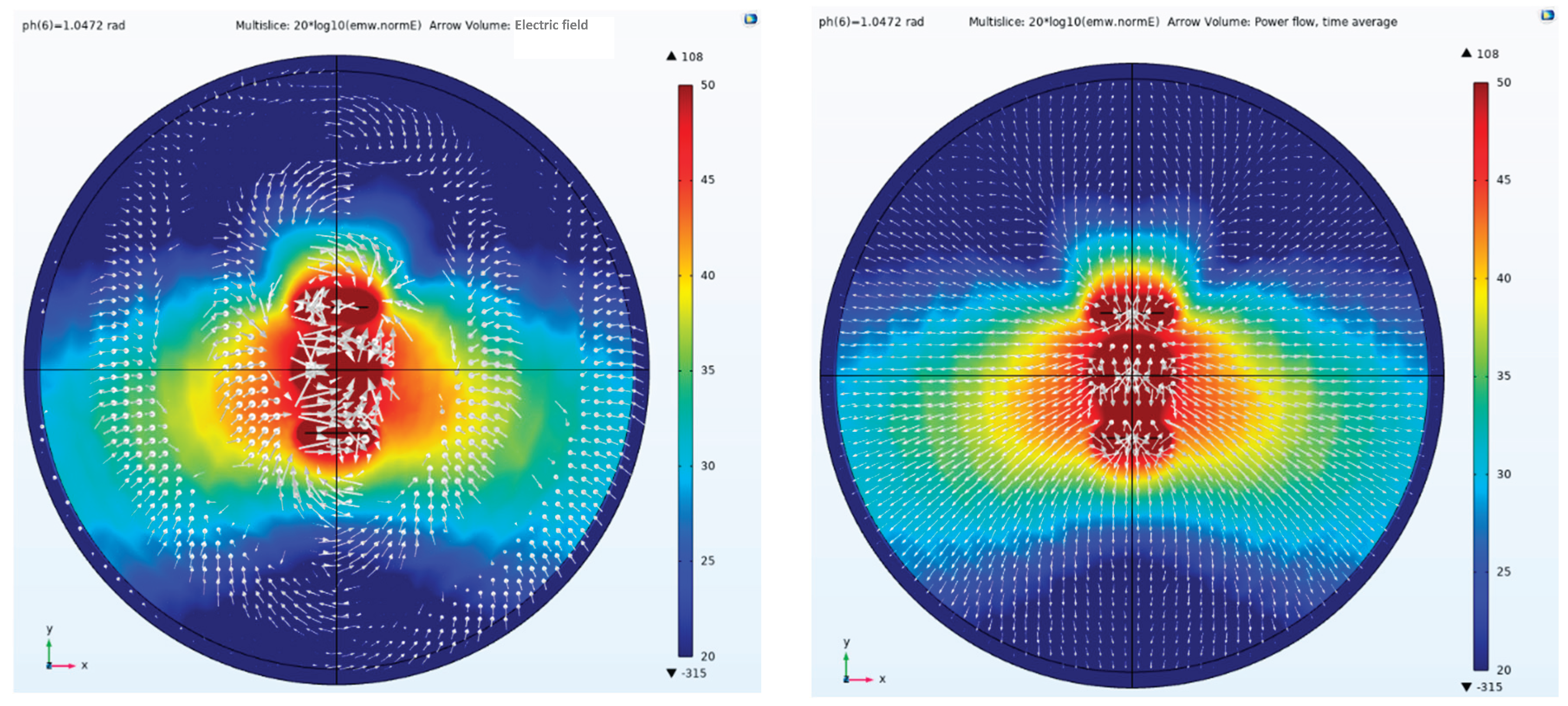
Figure 17.
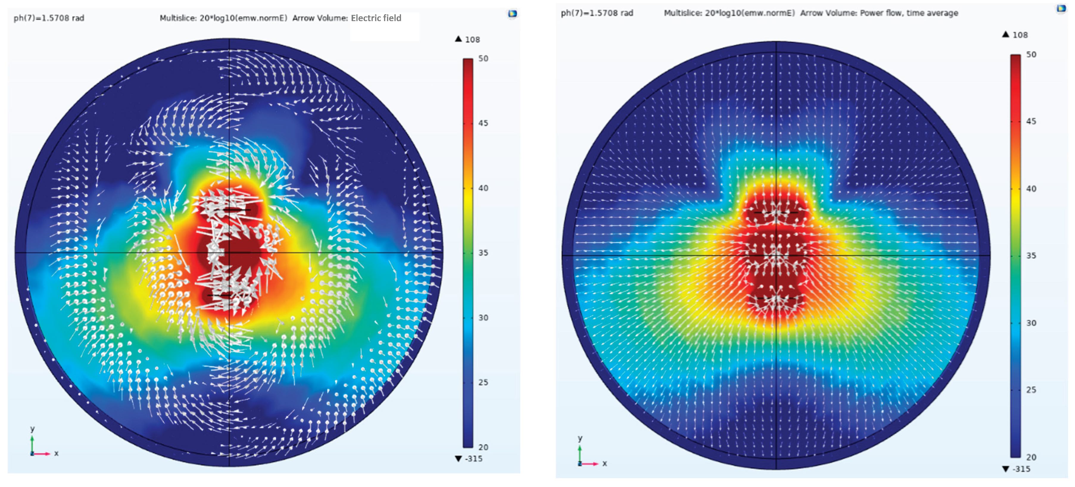
In the side view of the electric field amplitude, direction and Poynting vector arrow, the three antenna elements are excited by the Taylor synthesis and 1.5708 rad phase difference.
Figure 17.
In the side view of the electric field amplitude, direction and Poynting vector arrow, the three antenna elements are excited by the Taylor synthesis and 1.5708 rad phase difference.
The front-to-back ratio (F/B) of a directional antenna represents the ratio of the power flux density in the maximum radiation direction (defined as 0°) to the maximum power flux density in the opposite direction (defined as 180° ± 20°), as shown in Equation (24). This metric reflects the antenna's effectiveness in suppressing the rear lobe; a higher F/B value indicates less radiation (or reception) toward the rear.
where is the maximum power flux density in the radiation direction, and is the maximum flux density in the backward direction.
Table 2 shows the electric field values and F/B ratios generated by a 3×1 parallel dipole antenna array with different phase differences at various receiving points. When the phase difference is 0 rad, electromagnetic waves radiate uniformly in both directions. When the excitation phases on the three antenna elements are inconsistent, the electromagnetic waves will be deflected. Based on the F/B data in Table 2, the F/B increases almost proportionally as the phase difference increases.
As shown in Figure 18 and Figure 19, the E/H plane beam pattern exhibits different deflections at multiple phase differences. The greater the phase difference, the larger the deflection angle within a certain range. By adjusting the phase difference, the main beam direction can be aligned to point toward the region of interest. When phase excitation is applied via lumped ports using Taylor synthesis, the main lobe is symmetrically distributed along the antenna axis (light blue), and beam steering can be achieved by advancing the arithmetic phase (other colors).
The E-plane pattern reveals that the main beam completes the scanning process under excitation with varying phase differences. This process holds significant physical importance during CSAMT operations, enabling extensive scanning across the exploration area. Compared to traditional fixed-position exploration methods, it concentrates energy while achieving broad coverage. By moving only the receiver unit while keeping the transmitter stationary, large-area exploration with a high signal-to-noise ratio is accomplished—suitable for both general surveys and detailed exploration.
A well-designed antenna array should exhibit low side lobe levels, which are not readily apparent when plotted linearly. The V/m scale displayed in the 3D far-field patterns makes the main lobe and side lobes more visible, as shown in Figure 20 and Figure 21.
All of this demonstrates the feasibility of phase-difference weighted beamforming. During CSAMT surveys using parallel-element linear arrays, differential phase excitation enables the main radiation lobe to be directed toward regions of interest. Compared to the omnidirectional radiation of individual elements, this approach effectively enhances both the received field strength amplitude and SNR at receivers within the target area.
Table 3 presents numerical simulations of CSAMT adaptive beamforming based on an artificial field source using a parallel-element linear array under different phase differences. It can be observed that at the point (8000, 0, 0), as the phase difference changes from -1.5708 rad to 1.5708 rad in increments of 0.5236 rad, the numerical values exhibit a peak at the center and gradually decrease toward both sides. This fully demonstrates the beam scanning process: the electric field amplitude is highest when the main beam passes through the point (8000, 0, 0), and weakens at this point as the beam scans to either side. The points (8000, 4000, 0) and (8000, -4000, 0) also validate the beam scanning physics. At a phase difference of -1.5708 rad, the point (8000, 4000, 0) is highest, while the amplitude at point (8000, -4000, 0) is lowest. Conversely, when the phase difference is 1.5708 rad, the electric field amplitude at point (8000, -4000, 0) is highest, while the amplitude at point (8000, 4000, 0) is lowest.
Consistent with Table 3, Figure 22 also presents numerical simulations of CSAMT adaptive beamforming based on a parallel-element linear array artificial field source under varying phase differences. As the phase difference transitions from -1.5708 rad to 1.5708 rad, the main beam progressively scans from point (8000, 0, 0) through point (8000, 0, 0) to point (8000, -4000, 0). (8000, 4000, 0), through point (8000, 0, 0), and gradually scans to point (8000, -4000, 0).
4.5. Adaptive Beam Control Simulation for a Coaxial Dipole Field Source
Based on the model shown in Figure 8, a uniform half-space and 3×1 coaxial antenna array CSAMT model was established. Different phase and Taylor synthesis (502 V, 1055 V, and 502 V) excitations were applied to the three array elements with a 1 km arm length. Element 1's port phase was set to 0 rad. Element 2's port phase varied from -1.5708 rad to 1.5708 rad, changing every 0.5236 rad. Element 3's port phase variation was twice that of Element 2. Figure 23 depicts the 3×1 coaxial dipole antenna array with lumped ports. The phase difference between each lumped port is governed by a specific rule known as the arithmetic phase value, which controls the direction of the main lobe.
By performing the pH parameter scan shown in Table 4, the beam scanning capability of the 3×1 coaxial dipole antenna array can be obtained.
Figure 24 illustrates the case where three array elements are excited with identical phase. It can be seen that with identical phase excitation, the beam converges toward the center, with maximum energy concentrated along the centerline of the coaxial linear array. Conducting CSAMT surveys at this centerline position yields the highest signal-to-noise ratio.
Figure 25 shows a side view of the electric field amplitude, direction, and Poynting vector arrows. The array antenna is excited with a Taylor synthesis and a phase difference of -1.5708 rad. It can be observed that after applying the maximum phase difference excitation, the beam direction undergoes the greatest angular deviation. That is, the beam is effectively deflected according to the set parameters. The arrow direction indicates the direction of the Poynting vector, representing the propagation direction of energy. It is undeniable that after phase control through the array elements, the propagation direction of the electromagnetic wave has been altered.
Therefore, in actual exploration, even with a fixed artificial field source, the beam coverage can be significantly expanded. This breaks through the traditional 60° exploration range limitation of single-element dipole artificial field sources, extending the range to approximately 90°. Figure 26, Figure 27, Figure 28, Figure 29 and Figure 30 illustrate beam angle deflections under other phase differences.
As shown in Figure 31, the E-plane pattern exhibits different deflections at multiple phase differences. The greater the phase difference, the larger the deflection angle within a given range. By adjusting the phase difference, the main beam direction can be steered toward specific regions. When phase excitation is applied via lumped ports using Taylor synthesis, the main lobe exhibits symmetrical distribution along the antenna axis (light blue), and beam steering can be achieved by advancing the arithmetic phase (other colors).
Table 5 presents numerical simulations of CSAMT adaptive beamforming based on a coaxial linear array artificial field source at different phase differences. Similar to the parallel-element artificial field source, at the point (8000, 0, 0), as the phase difference varies from -1.5708 rad to 1.5708 rad in 0.5236 rad increments, the values exhibit a peak at the center and gradually decrease toward the edges. The electric field amplitude reaches its maximum when the main beam passes through the point (8000, 0, 0), and weakens at this point as the beam sweeps to either side. The behavior at points (8000, 4000, 0) and (8000, -4000, 0) also aligns with parallel dipoles. When the phase difference is -1.5708 rad, the electric field amplitude peaks at point (8000, 4000, 0) and reaches its minimum at point (8000, -4000, 0). Conversely, when the phase difference is 1.5708 rad, the electric field amplitude peaks at point (8000, -4000, 0) and reaches its minimum at point (8 0) is highest, while the amplitude at point (8000, -4000, 0) is lowest. Conversely, when the phase difference is 1.5708, the electric field amplitude at point (8000, -4000, 0) is highest, while the amplitude at point (8000, 4000, 0) is lowest.
Consistent with the parallel dipole artificial source, Figure 32 also presents numerical simulations of CSAMT adaptive beamforming based on a coaxial dipole linear array artificial source under varying phase differences. As the phase difference transitions from -1.5708 rad to 1.5708 rad, the main beam progressively scans from point (8000, 0, 0) through point (8000, 0, 0) to point (8000, -4000, 0). (8000, 4000, 0), through point (8000, 0, 0), and gradually scans to point (8000, -4000, 0).
5. Prototype Implementation
5.1. Principle of GPS Time Synchronization
Remote time synchronization between transmitter units and receiver units is achieved using the Global Positioning System (GPS). This method is not only simple to operate but also highly accurate, enabling independent operation of transmitter units and receiver units, making it suitable for field construction. Figure 33 illustrates the schematic diagram of GPS time synchronization between transmitter units and receiver units.
The GPS continuously provides highly accurate time parameters to users worldwide, enabling users in all regions to receive uniformly standardized Coordinated Universal Time (UTC). When ground equipment receives sufficient satellite signals and successfully locks onto satellite positions, it can reliably obtain precise time code data provided by GPS. Transmitter units and receiver units located in different geographical positions can both successfully acquire satellite signals. By decoding and calibrating the reference time provided by GPS, strict time synchronization among multiple devices can be achieved.
5.2. Time Synchronization System Design
In environments with severe obstructions, such as deep mountains and dense forests, transmitter clusters and receiver units face the risk of “satellite loss.” Should satellite loss occur, it will introduce significant errors into the system's time synchronization and may even disrupt normal system operation. To address this issue, the time synchronization system in this study employs GPS time as the basis for “satellite acquisition.” During satellite loss, transmitter clusters and receiver units can synchronize using the high-precision time reference signal generated by the local time synchronization system. Upon GPS signal restoration, the local system automatically reverts to GPS timing mode. This approach effectively mitigates GPS signal instability, ensuring accurate and stable time synchronization.
The components of the time synchronization system in this study primarily include: a local clock module, an FPGA second pulse generation and processing module, a GPS module, a DSP data processing module, and a human-machine interface module. Figure 34 presents the block diagram of the transmitter GPS time synchronization device.
After the GPS receiver unit successfully locks onto satellites, it transmits the generated second pulse signal to the FPGA module. The second pulse processing module, which performs logic analysis and filtering, enables reliable and stable 1PPS signal output. Simultaneously, serial data is transmitted to the DSP module for decoding, yielding UTC data. Upon detecting the rising edge of the filtered second pulse signal, precise UTC information is uploaded via the serial port to the host computer for display. Moreover, the voltage-controlled oven-controlled crystal oscillator (VC-OCXO) generates a local clock signal. This signal requires calibration via the precise second pulse signal and is processed through a frequency multiplier module to generate a high-precision second pulse signal. During satellite loss events, this signal can replace the GPS second pulse signal, ensuring time synchronization for the array antenna system.
5.3. Phase Control System Implementation
When synthesizing and scanning beam patterns using array antennas, precise management of the excitation amplitude and phase of each antenna element within the array is essential, particularly phase control. This system primarily employs two phase control methods based on the type of output waveform. The Different Phases-Same Time (DPST) system is employed for phase control of sine wave outputs, while the Same Phases-Different Time (SPDT) system is used for phase modulation of square wave outputs.
5.3.1. DPST System
During phase control, the transmission timing of all transmitters is synchronized and unified, while the initial phase of each transmitter is managed asynchronously. By adjusting the phase, the objective of phase control is achieved. The DPST control system primarily employs Direct Digital Synthesis (DDS) technology to perform phase modulation on the output SPWM.
Sine-Pulse Width Modulation (SPWM) refers to pulse widths varying according to a sine function. Its principle is based on the impulse equivalence principle: on inertial links, narrow pulses with equal impulse but different shapes produce essentially identical effects. Impulse is the integral area of a narrow pulse, and “essentially identical effects” means the link's output waveforms are fundamentally similar. When analyzing each input waveform via Fourier transform, the low-frequency segments are highly similar, with only slight differences appearing in the high-frequency portions.
Direct Digital Synthesis (DDS) is a digital synthesis technique that converts a series of digital signals into analog signals via a digital-to-analog converter (DAC). DDS employs two fundamental synthesis methods: lookup table and computational. This paper adopts the DDS lookup table method, with Figure 35 illustrating its principle.
In SPWM, an isosceles triangular wave is used as the carrier wave. This waveform is characterized by a linear relationship between the horizontal width and height at any point, along with bilateral symmetry. When the isosceles triangular wave intersects with any gradually varying modulation signal wave, switching devices in the control circuit can be activated to open or close at the intersection point, thereby generating pulses whose width is proportional to the amplitude of the signal wave. When the modulating signal wave is a sine wave, the resulting waveform is the SPWM waveform. Here, we set the sine wave period to ten times that of the triangle wave. By comparing the amplitudes of the triangle wave and sine wave, the SPWM signal is 0 when the triangle wave is greater than the sine wave, and 1 otherwise. This generates an SPWM waveform with irregular duty cycles. Figure 36 shows the comparison curves of the triangle carrier and the sine wave.
Mapping a sine wave onto a circle using a 32-bit phase accumulator can be understood as dividing the circumference into 232 equal segments, ranging from 0 to 232-1. When starting with an initial value of 0 added to the phase accumulator, the sine wave begins outputting from a phase of 0. Therefore, by adding any initial value to the phase accumulator at the start, the waveform can begin outputting from any desired phase. The initial value loaded into the phase accumulator at startup is the initial phase control word. Suppose we want the sine wave to output from a phase of . On the circle, this corresponds to the 180° position, which is the midpoint of the circle's phase. This is because the number of bits in the phase accumulator determines how many equal divisions the circle has. If the circle is divided into 232 equal segments, 180° corresponds to the midpoint between 0 and 232-1. Therefore, set the initial phase control word to 232/2 = 231. To start waveform output from a phase of 90°, this corresponds to the quarter position on the circle, i.e., one-quarter of the range from 0 to 232-1. The initial phase accumulator value can be set to 232/4 = 230. Other positions are calculated similarly. Figure 37 shows the FPGA implementation of the DDS lookup table method.
The current lookup table method achieves access to waveform data by pre-storing the output waveform data (sine function table) in ROM cells. The address input of the ROM cells is connected to a counter, enabling the counter to generate the addresses required for accessing the sine wave data. Subsequently, data is read from the ROM cells in a specific sequence at a clock frequency that has been divided down.
Through modular system design, the FPGA module circuit (EP2C8Q208) and DSP module circuit (TMS320F28335) were designed independently. Subsequently, these module circuits were integrated within the power conditioning module circuit. Figure 38 shows the physical diagram of the phase control board.
5.3.2. SPDT System
The implementation of the SPDT control system is simpler than that of the DPST system, as it does not require management of the initial phase of the transmitter array and receiving units, all of which are set to 0° phase. Instead, the transmission timing of the transmitter array is managed asynchronously. After the VC-OCXO crystal oscillator generates the local clock signal, it must be calibrated using an accurate pulse-per-second (PPS) signal. A frequency multiplication module is then employed to generate a high-precision PPS signal. In this system, the frequency multiplication module multiplies the 1PPS signal by 1000 ms. These 1000 ms () correspond to a 360° phase shift. To achieve a 90° phase difference between two adjacent transmitters, a transmission time difference of between the two transmitters is sufficient. Similarly, to achieve a 60° phase difference, a transmission time offset of can be applied.
6. Adaptive Beamforming Experiment for a Linear Array Field Source
6.1. Adaptive Beamforming Test with Parallel Dipole Field Source
Figure 39 illustrates the adaptive beamforming layout for a parallel-dipole linear array artificial field source. The transmitter configuration remains consistent with the preceding description. After synthesizing the directional patterns of the parallel-dipole linear array and applying different phases, the main beam will scan with a phase. As illustrated, the green region represents the conventional “zero zone.” As discussed in the previous section, measurements within the zero zone—whether using a single dipole artificial field source, a parallel dipole linear array artificial field source, or a coaxial dipole linear array artificial field source—fall outside the exploration range both before and after pattern synthesis. Consequently, data acquired in this zone is unusable. This section applies adaptive beam control technology to adjust the beam direction. During actual exploration, the beam direction can be modified based on phase difference changes. This allows the beam to include the “zero zone” during scanning, thereby expanding the exploration range.
Figure 40 illustrates the phase difference scan of three elements in a parallel-element linear array artificial field source, with each element excited sequentially according to the parameterization. Each phase difference is held for 1 minute. After the receiving unit completes data acquisition, it moves to the next phase difference. The electric field values at the coaxial adaptive measurement point are then recorded. The transmitter operates at frequencies of 16 Hz and 2560 Hz. The trend is consistent: when the beam is directed toward the coaxial adaptive measurement point, the electric field amplitude reaches its maximum value. When directed elsewhere, the amplitude decays relative to the maximum value.
Figure 41 shows the electric field amplitude at the zero-zone adaptive measurement point during main beam movement. It can be observed that when the main beam moves within the exploration range of the single-dipole antenna artificial field source (yellow area in the figure), the electric field values at the zero-zone adaptive measurement point exhibit significant errors, rendering the recorded data unreliable. This aligns with the previously mentioned zero-zone measurement values. When the beam scans the zero zone, the electric field data recorded by the zero-zone adaptive measurement point stabilizes, with the amplitude matching the values from numerical simulations. The practical significance of this process is that beam scanning significantly expands the exploration range of CSAMT, effectively eliminating the zero zone across the entire area.
6.2. Adaptive Beamforming Test for Coaxial Dipole Field Source
Figure 42 shows the adaptive beamforming layout for a coaxial vibrator linear array artificial source.
As shown, the transmitter layout is consistent with the previous configuration. After synthesizing the radiation patterns of the coaxial vibrator linear array and applying distinct phase differences to each of the three array elements, the main beam will scan with the phase difference.
Similar to the parallel-element linear array artificial field source, Figure 43 illustrates the phase difference between three sequentially excited elements in a coaxial-element linear array artificial field source, scanned according to parameterization. Each phase difference is held for 1 minute. After the receiving unit completes data acquisition, it moves to the next phase difference. The electric field values at the centerline adaptive measurement point are then recorded. The transmitter operates at frequencies of 16 Hz and 2560 Hz. The trends are consistent: when the beam is directed toward the centerline adaptive measurement point, the electric field amplitude reaches its maximum value. When directed elsewhere, the amplitude decays relative to the maximum value.
Figure 44 shows the electric field amplitude at the zero-zone adaptive measurement point during the main beam's movement. It can be observed that when the main beam is within the zero-zone range, the electric field value data recorded by the zero-zone adaptive measurement point remains stable, and the amplitude of the electric field values aligns with the values from the numerical simulation. When the main beam moves into the exploration range of the single dipole antenna artificial field source (blue area in the figure), the error in the electric field values recorded by the zero-zone adaptive measurement point gradually increases, rendering the recorded data meaningless. This also aligns with the zero-zone measurement values discussed earlier. The practical significance of this process is that through beam scanning, the exploration range of CSAMT can be significantly expanded, meaning there is no zero zone across the entire area.
7. Conclusions
Based on the analysis of array antenna principles and utilizing a linear array model, the CSAMT's coaxial dipole array antenna and parallel dipole array antenna artificial field sources were designed. Dolph-Chebyshev synthesis and Taylor synthesis methods were applied to perform low-side lobe synthesis on the CSAMT's radiation pattern, minimizing side lobe levels while maintaining a specified main lobe width. Simulation results, numerical modeling, and field tests demonstrate that the application of linear array artificial field sources combined with synthesis methods can significantly reduce side lobe levels, markedly enhance main lobe energy density, and decrease interference from side lobes at the receiving point.
Through an analysis of the principles behind beam scanning and adaptive beamforming methods, we designed an adaptive beamforming approach for CSAMT based on a linear array artificial ground source. By processing the electric field data at the receiver end and applying the maximum amplitude principle, the parameters of the array transmitter antenna can be adaptively locked to achieve the maximum signal-to-noise ratio for data reception. A model was established to perform numerical simulations of the adaptive beamforming method. Simulation results, numerical simulations, and field test results have validated the feasibility of this method.
Author Contributions
Conceptualization, H.F.; methodology, H.F.; visualization, X.S.; project administration, Q.T.; validation, X.S.; Q.S. All authors have read and agreed to the published version of the manuscript.
Funding
This work was supported by the Tianjin Technology Innovation Guidance Special Project (Fund) - Enterprise Science and Technology Commissioner Project. (No. 25YDTPJC00870)
Institutional Review Board Statement
Not applicable.
Informed Consent Statement
Not applicable.
Data Availability Statement
Not applicable.
Acknowledgments
All of the authors thank the referees, editors, and officers of Symmetry for their valuable suggestions and help.
Conflicts of Interest
The authors declare no conflicts of interest.
Abbreviations
| CSAMT | Controlled-source audio-frequency magnetotelluric |
| AMT | Audio-Frequency Magnetotellurics |
| MT | Magnetotellurics |
| MRC | Maximum Ratio Combining |
| GPR | Ground-penetrating radar |
| SNR | Signal to Noise Ratio |
| DPST | Different Phases-Same Time |
| SPDT | Same Phases-Different Time |
| DDS | Direct Digital Synthesis |
| SPWM | Sine-Pulse Width Modulation |
References
- Wang X X, Di Q Y, Xu C. Characteristics of multi-dipole sources and tensor measurements of CSAMT[J]. Chinese Journal of Geophysics 2014, 57, 651–661. [Google Scholar]
- Unsworth, M.J.; Lu, X.; Watts, M.D. CSAMT exploration at Sellafield: Characterization of a potential radioactive waste disposal site. Geophysics 2000, 65, 1070–1079. [Google Scholar] [CrossRef]
- Fu, C.; Di, Q.; An, Z. Application of the CSAMT method to groundwater exploration in a metropolitan environment. Geophysics 2013, 78, B201–B209. [Google Scholar] [CrossRef]
- Guo, Z.; Hu, L.; Liu, C.; Cao, C.; Liu, J.; Liu, R. Application of the CSAMT Method to Pb–Zn Mineral Deposits: A Case Study in Jianshui, China. Minerals 2019, 9, 726. [Google Scholar] [CrossRef]
- Boerner, D.E.; Kurtz, R.D.; Jones, A.G. Orthogonality in CSAMT and MT measurements. Geophysics 1993, 58, 924–934. [Google Scholar] [CrossRef]
- Wu, G.; Hu, X.; Huo, G.; Zhou, X. Geophysical exploration for geothermal resources: An application of MT and CSAMT in Jiangxia, Wuhan, China. J. Earth Sci. 2012, 23, 757–767. [Google Scholar] [CrossRef]
- Spichak, V.; Fukuoka, K.; Kobayashi, T.; Mogi, T.; Popova, I.; Shima, H. ANN reconstruction of geoelectrical parameters of the Minou fault zone by scalar CSAMT data. J. Appl. Geophys. 2002, 49, 75–90. [Google Scholar] [CrossRef]
- An, Z.; Di, Q. Investigation of geological structures with a view to HLRW disposal, as revealed through 3D inversion of aeromagnetic and gravity data and the results of CSAMT exploration. J. Appl. Geophys. 2016, 135, 204–211. [Google Scholar] [CrossRef]
- Wannamaker, P.E. Tensor CSAMT survey over the Sulphur Springs thermal area, Valles Caldera, New Mexico, United States of America, Part I: Implications for structure of the western caldera. Geophysics 1997, 62, 451–465. [Google Scholar] [CrossRef]
- Guan Z W, Li T L, Zhu C, et al. CSAMT simulation study of 3D geological models[J]. Progress in Geophysics 2016, 31, 1073–1079. [Google Scholar]
- Chen, J.; Li, Z.; Tian, B.; Chen, X.; Zheng, J.; Zhang, C.; Zhao, W.; Zhang, F. Using the CSAMT method to predict deep mineralisation of copper and molybdenum: a case study of the Zhongxingtun area in Inner Mongolia, China. Explor. Geophys. 2019, 51, 203–213. [Google Scholar] [CrossRef]
- Michael, M.W.; Michael, V.; Rutter, H.; Cull, J.P. An All-Frequency Resistivity-Depth and Static-Correction Technique for CSAMT Data, with Applications to Mineralised Targets under Glacial Cover (Western Tasmania) and Basalt Cover (Victorian Goldfields). Explor. Geophys. 2005, 36, 287–293. [Google Scholar] [CrossRef]
- Park M K, Seol S J, Kim H J. Sensitivities of generalized RRI method for CSAMT survey[J]. Geosciences Journal 2006, 10, 75–84. [Google Scholar] [CrossRef]
- Yu C, M. Application of the CSAMT method in prospecting for concealed gold deposits[J]. Chinese Journal of Geophysics 1998, 41, 133–138. [Google Scholar]
- Li D Q, Hu Y F. Comparison of detection effects between wide-area electromagnetic method and CSAMT in high-interference mining areas[J]. Geophysical and Geochemical Exploration 2015, 39, 967–972. [Google Scholar]
- Farhat N H, Bai B. Phased-array antenna pattern synthesis by simulated annealing[J]. Proceedings of the IEEE 1987, 75, 842–844. [Google Scholar] [CrossRef]
- Guo J L, Li J Y. Pattern synthesis of conformal array antenna in the presence of platform using differential evolution algorithm[J]. IEEE Transactions on Antennas and Propagation 2009, 57, 2615–2621. [Google Scholar] [CrossRef]
- Lebret, H.; Boyd, S. Antenna array pattern synthesis via convex optimization. IEEE Trans. Signal Process. 1997, 45, 526–532. [Google Scholar] [CrossRef]
- Mautz, J.; Harrington, R. Computational methods for antenna pattern synthesis. IEEE Trans. Antennas Propag. 1975, 23, 507–512. [Google Scholar] [CrossRef]
- Ferreira J A, Ares F. Pattern synthesis of conformal arrays by the simulated annealing technique[J]. Electronics Letters 1997, 33, 1187–1189. [Google Scholar] [CrossRef]
- Perini, J.; Idselis, M. Note on antenna pattern synthesis using numerical iterative methods. IEEE Trans. Antennas Propag. 1971, 19, 284–286. [Google Scholar] [CrossRef]
- Steyskal, H. Synthesis of antenna patterns with prescribed nulls. IEEE Trans. Antennas Propag. 1982, 30, 273–279. [Google Scholar] [CrossRef]
- Ismail, T.H.; Abu-Al-Nadi, D.I.; Mismar, M.J. Phase-Only Control for Antenna Pattern Synthesis of Linear Arrays Using the Levenberg-Marquardt Algorithm. Electromagnetics 2004, 24, 555–564. [Google Scholar] [CrossRef]
- Li W T, Shi X W, Hei Y Q, et al. A hybrid optimization algorithm and its application for conformal array pattern synthesis[J]. IEEE Transactions on Antennas and Propagation 2010, 58, 3401–3406. [Google Scholar] [CrossRef]
- Lu, C.; Sheng, W.; Han, Y.; Ma, X. Phase-only pattern synthesis based on gradient-descent optimization. J. Syst. Eng. Electron. 2016, 27, 297–307. [Google Scholar] [CrossRef]
- Lei, S.; Hu, H.; Chen, B.; Tian, J.; Tang, P.; Qiu, X. Power Gain Pattern Synthesis for Wide-Beam Array Antenna via Linear Programming. IEEE Antennas Wirel. Propag. Lett. 2020, 19, 2300–2304. [Google Scholar] [CrossRef]
- Liang, J.; Fan, X.; Fan, W.; Zhou, D.; Li, J. Phase-Only Pattern Synthesis for Linear Antenna Arrays. IEEE Antennas Wirel. Propag. Lett. 2017, 16, 3232–3235. [Google Scholar] [CrossRef]
- Shi, Z.; Feng, Z. A new array pattern synthesis algorithm using the two-step least-squares method. IEEE Signal Process. Lett. 2005, 12, 250–253. [Google Scholar] [CrossRef]
- Ma, Y.; Yang, S.; Chen, Y.; Qu, S.-W.; Hu, J. Pattern Synthesis of 4-D Irregular Antenna Arrays Based on Maximum-Entropy Model. IEEE Trans. Antennas Propag. 2019, 67, 3048–3057. [Google Scholar] [CrossRef]
- Alizadeh, M.M.; Hosseini, S.E. Pattern synthesize of a cylindrical conformal array antenna by PSO algorithm. Int. J. RF Microw. Comput. Eng. 2020, 30. [Google Scholar] [CrossRef]
- Nilsen, C.-I.; Hafizovic, I. Beamspace adaptive beamforming for ultrasound imaging. IEEE Trans. Ultrason. Ferroelectr. Freq. Control. 2009, 56, 2187–2197. [Google Scholar] [CrossRef]
- Elnashar, A.; Elnoubi, S.M.; El-Mikati, H.A. Further Study on Robust Adaptive Beamforming With Optimum Diagonal Loading. IEEE Trans. Antennas Propag. 2006, 54, 3647–3658. [Google Scholar] [CrossRef]
- Chen, S.; Sun, S.; Gao, Q.; Su, X. Adaptive Beamforming in TDD-Based Mobile Communication Systems: State of the Art and 5G Research Directions. IEEE Wirel. Commun. 2016, 23, 81–87. [Google Scholar] [CrossRef]
- Zhou, C.; Gu, Y.; He, S.; Shi, Z. A Robust and Efficient Algorithm for Coprime Array Adaptive Beamforming. IEEE Trans. Veh. Technol. 2017, 67, 1099–1112. [Google Scholar] [CrossRef]
- Khabbazibasmenj, A.; Vorobyov, S.A.; Hassanien, A. Robust Adaptive Beamforming Based on Steering Vector Estimation With as Little as Possible Prior Information. IEEE Trans. Signal Process. 2012, 60, 2974–2987. [Google Scholar] [CrossRef]
- Blomberg, A.E.A.; Austeng, A.; Hansen, R.E.; Synnes, S.A.V. Improving Sonar Performance in Shallow Water Using Adaptive Beamforming. IEEE J. Ocean. Eng. 2013, 38, 297–307. [Google Scholar] [CrossRef]
- Liao, B.; Guo, C.; Huang, L.; Li, Q.; So, H.C. Robust Adaptive Beamforming With Precise Main Beam Control. IEEE Trans. Aerosp. Electron. Syst. 2017, 53, 345–356. [Google Scholar] [CrossRef]
- Gu, Y.; Leshem, A. Robust Adaptive Beamforming Based on Interference Covariance Matrix Reconstruction and Steering Vector Estimation. IEEE Trans. Signal Process. 2012, 60, 3881–3885. [Google Scholar] [CrossRef]
- Zhang, M.; Zhang, A.; Yang, Q. Robust Adaptive Beamforming Based on Conjugate Gradient Algorithms. IEEE Trans. Signal Process. 2016, 64, 6046–6057. [Google Scholar] [CrossRef]
- Pei, X.; Yin, H.; Tan, L.; Cao, L.; Li, Z.; Wang, K.; Zhang, K.; Bjornson, E. RIS-Aided Wireless Communications: Prototyping, Adaptive Beamforming, and Indoor/Outdoor Field Trials. IEEE Trans. Commun. 2021, 69, 8627–8640. [Google Scholar] [CrossRef]
Figure 1.
Finite length dipole antenna, where .
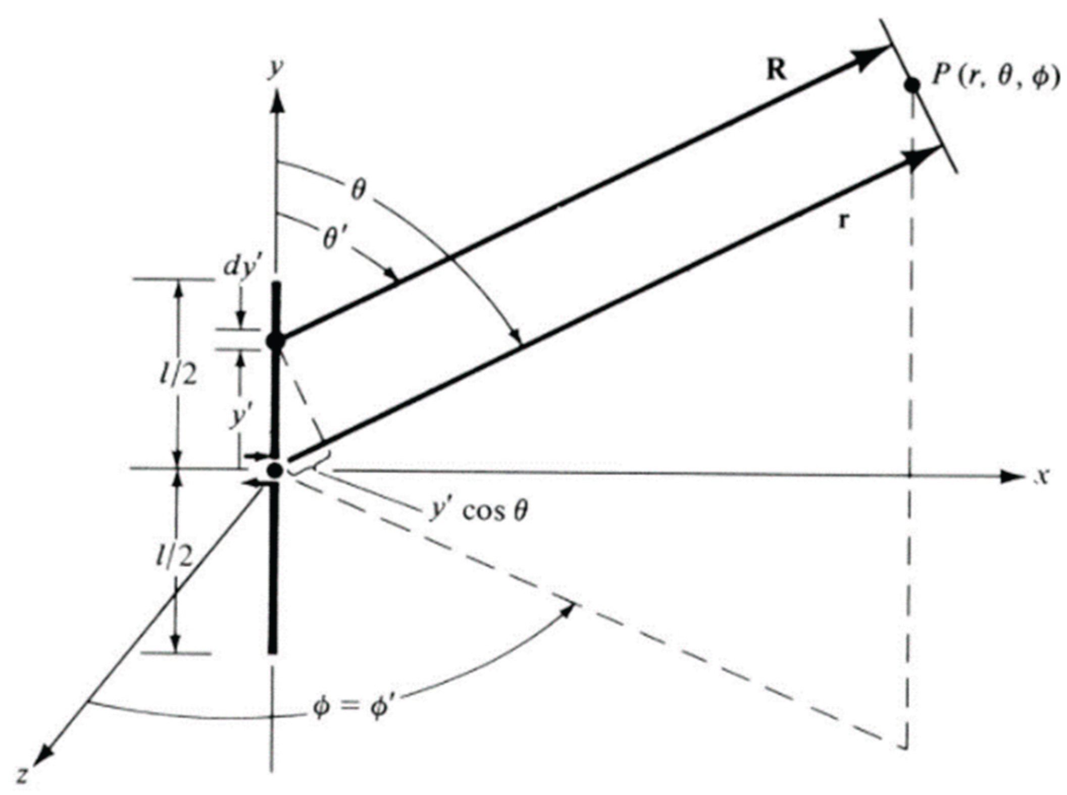
Figure 2.
Finite length dipole antenna, where .
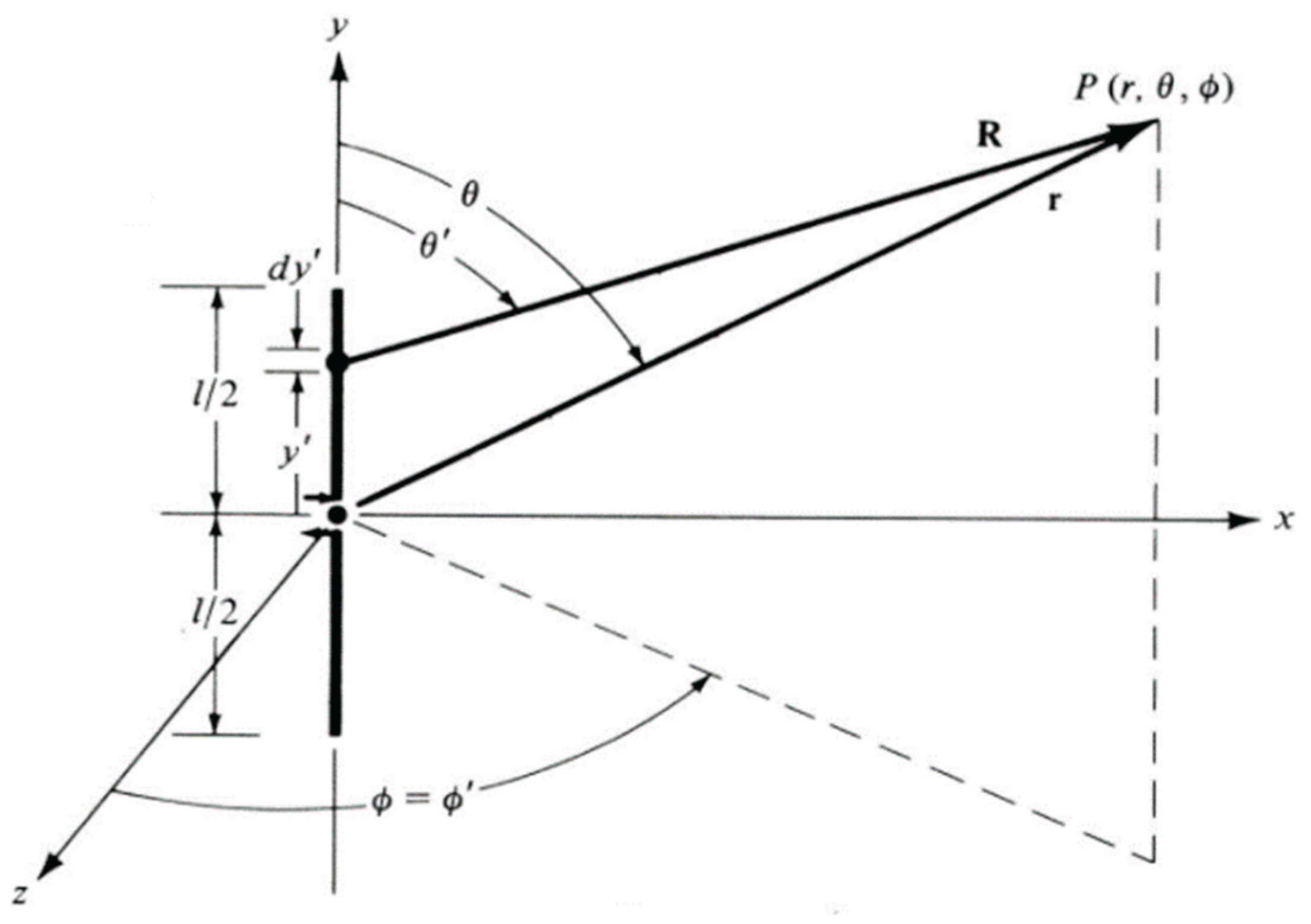
Figure 3.
Uniform linear array.
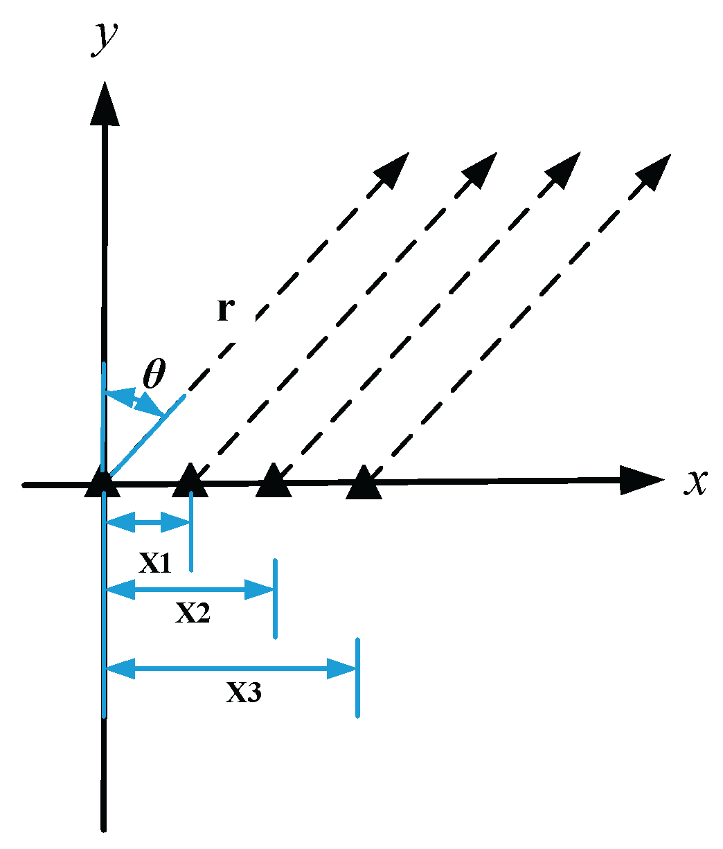
Figure 4.
Maximum ratio combination principle.
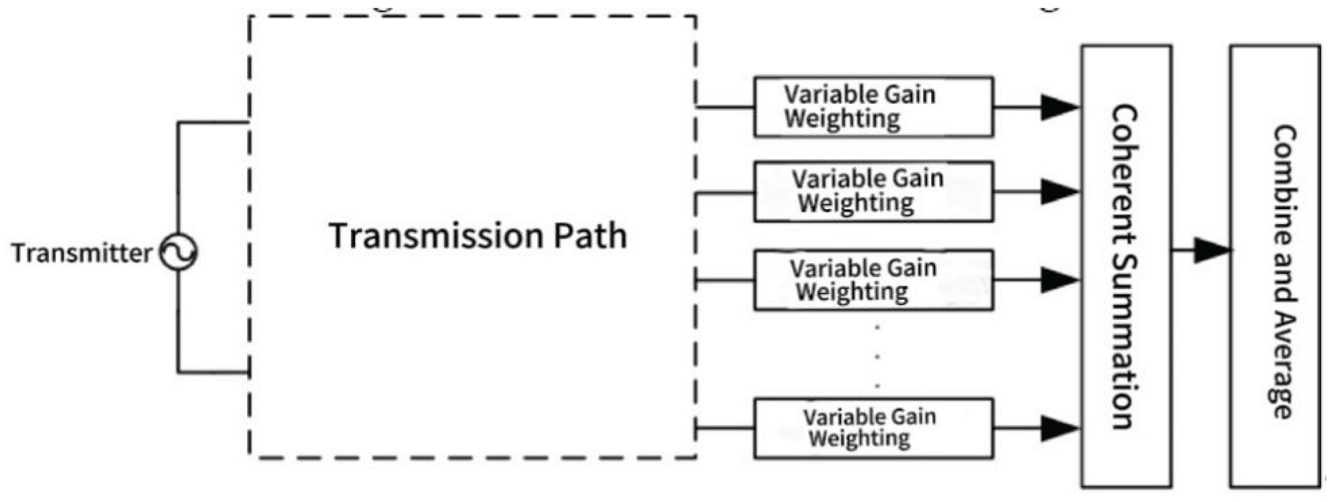
Figure 5.
Parallel vibrator linear array.

Figure 6.
CSAMT model of 3×1 parallel vibrator linear array.
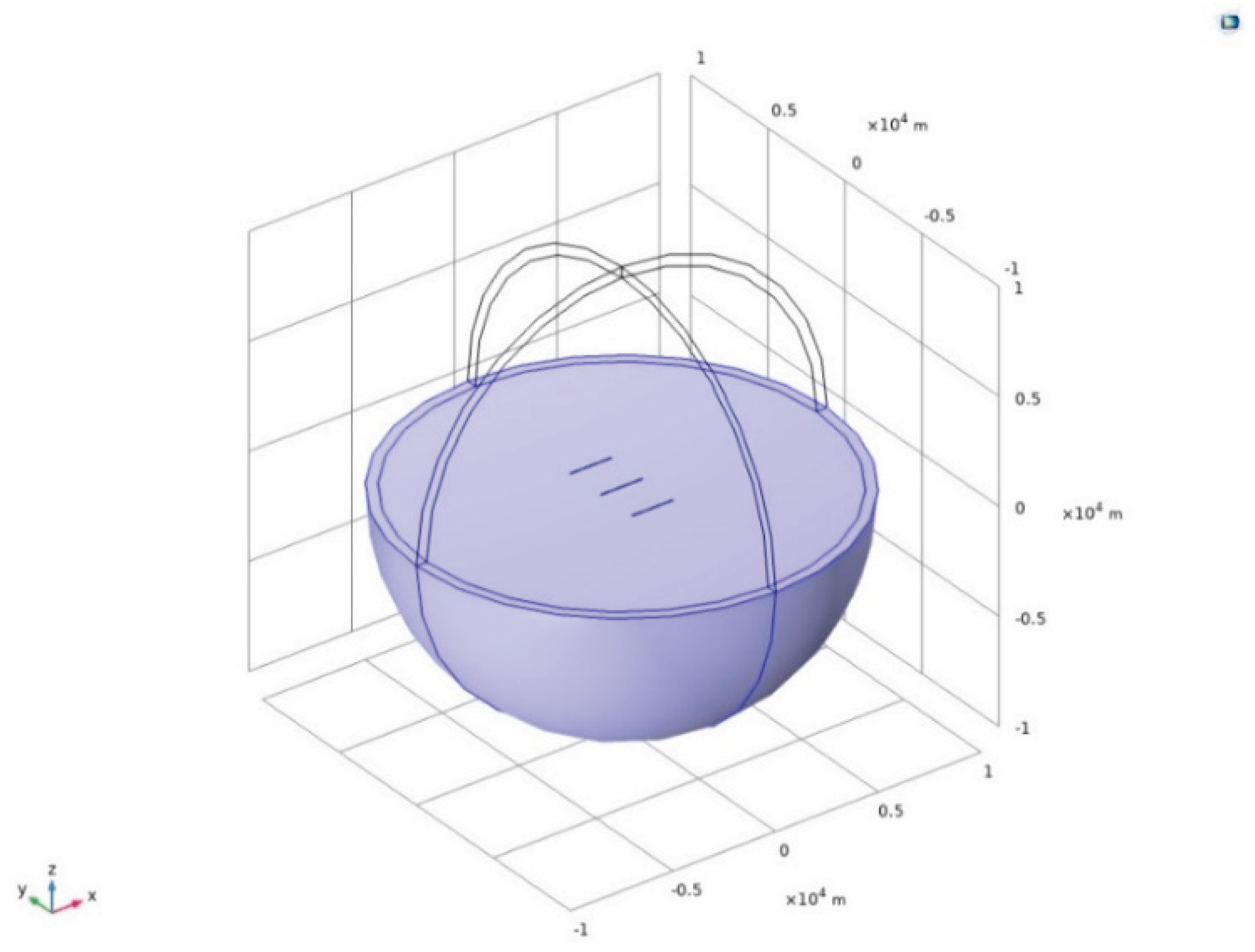
Figure 7.
Coaxial vibrator linear array.
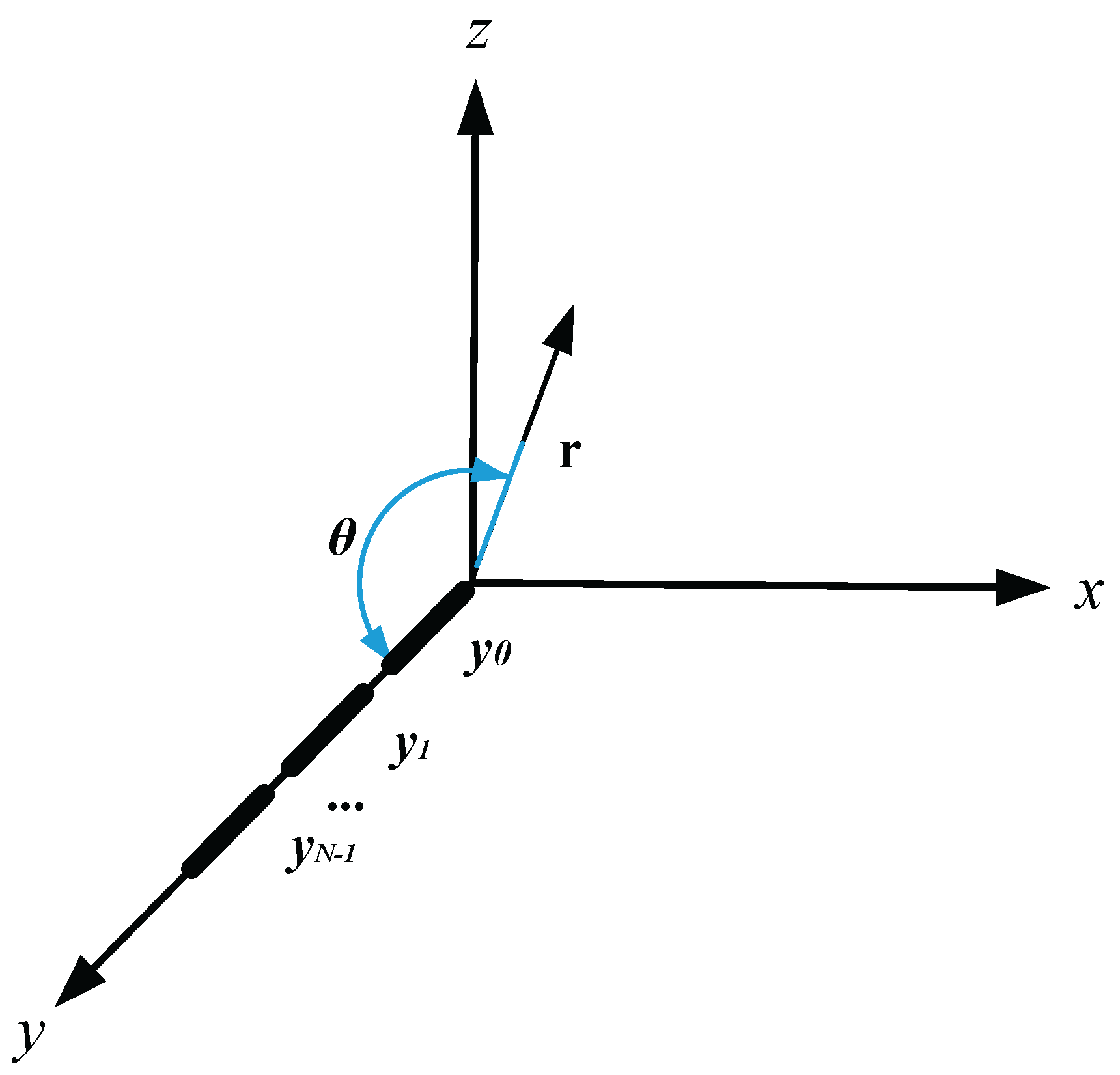
Figure 8.
3×1 CSAMT model of coaxial vibrator linear array.
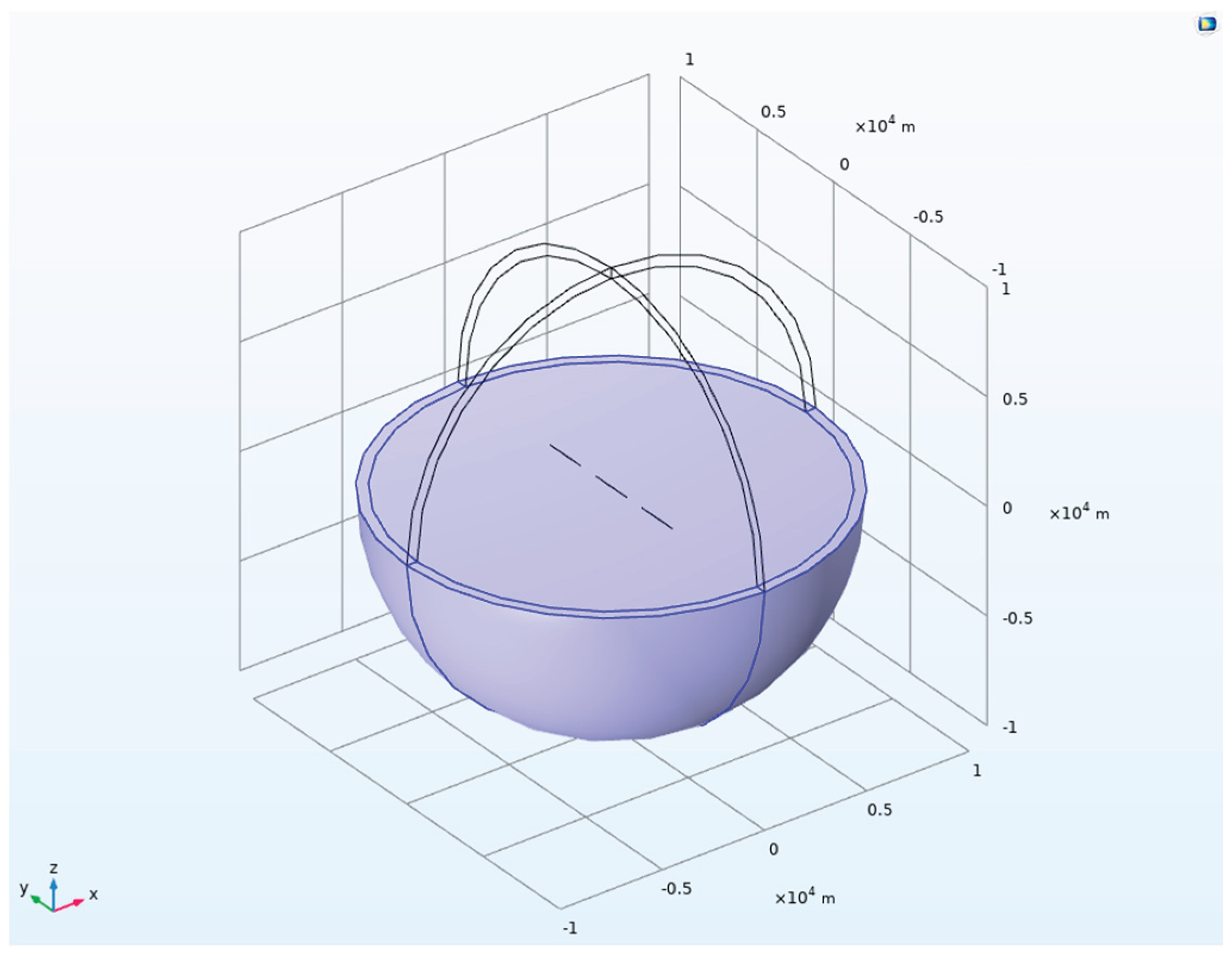
Figure 9.
Parallel dipole 3×1antenna array lumped port.
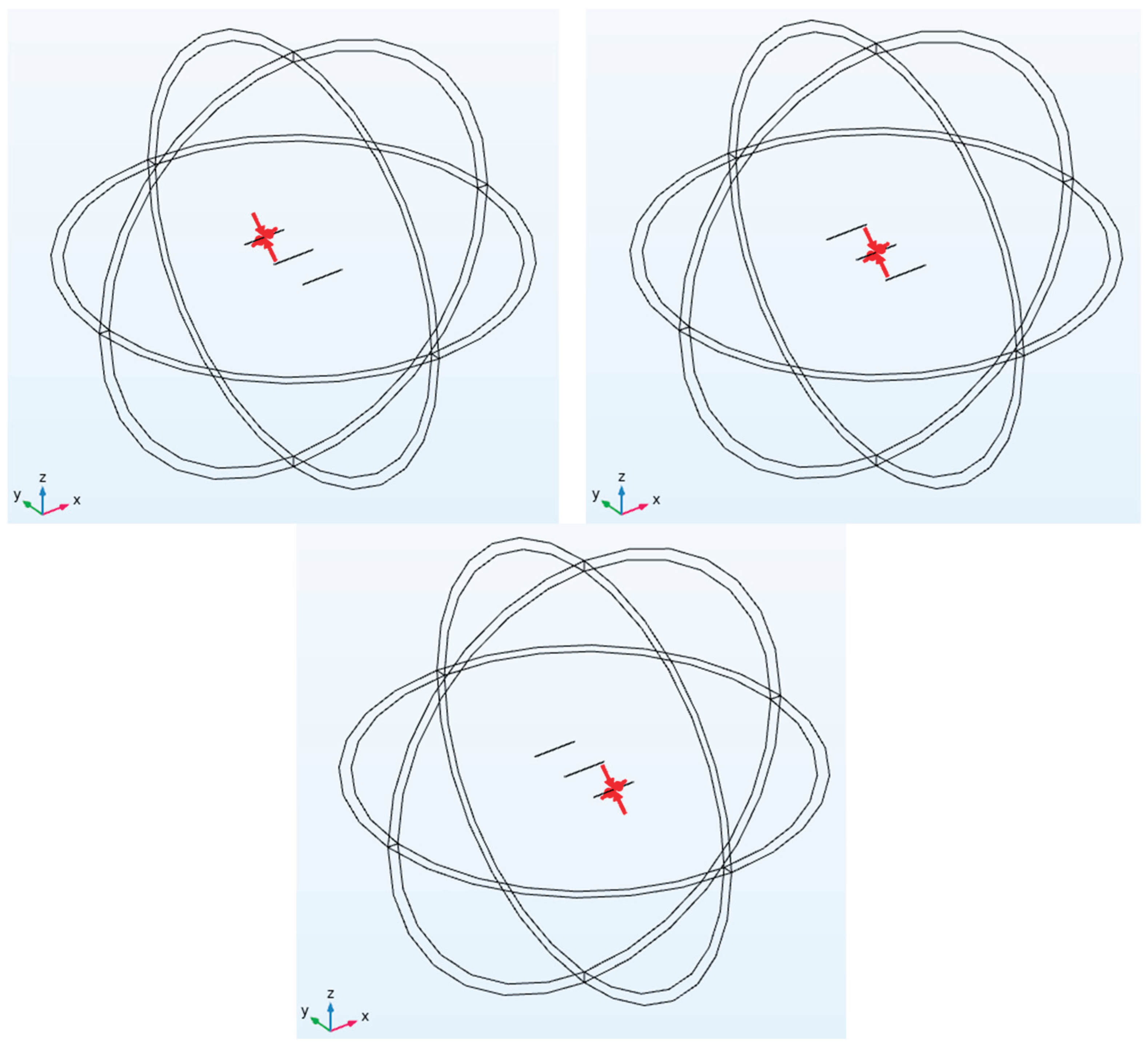
Figure 10.
In the side view of electric field amplitude, direction, three array element antennas are excited by the same phase (0 rad).
Figure 10.
In the side view of electric field amplitude, direction, three array element antennas are excited by the same phase (0 rad).
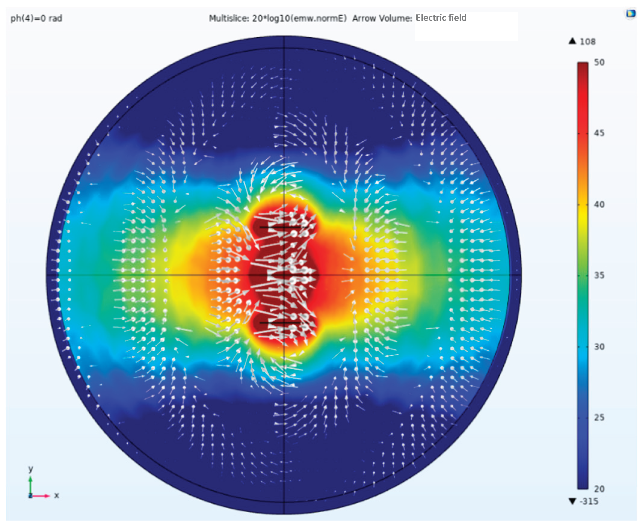
Figure 11.
In the side view of Poynting vector arrow, three array element antennas are excited by the same phase (0 rad).
Figure 11.
In the side view of Poynting vector arrow, three array element antennas are excited by the same phase (0 rad).

Figure 12.
In the side view of the electric field amplitude, direction and Poynting vector arrow, the three antenna elements are excited by the Taylor synthesis and -1.5708 rad phase difference.
Figure 12.
In the side view of the electric field amplitude, direction and Poynting vector arrow, the three antenna elements are excited by the Taylor synthesis and -1.5708 rad phase difference.
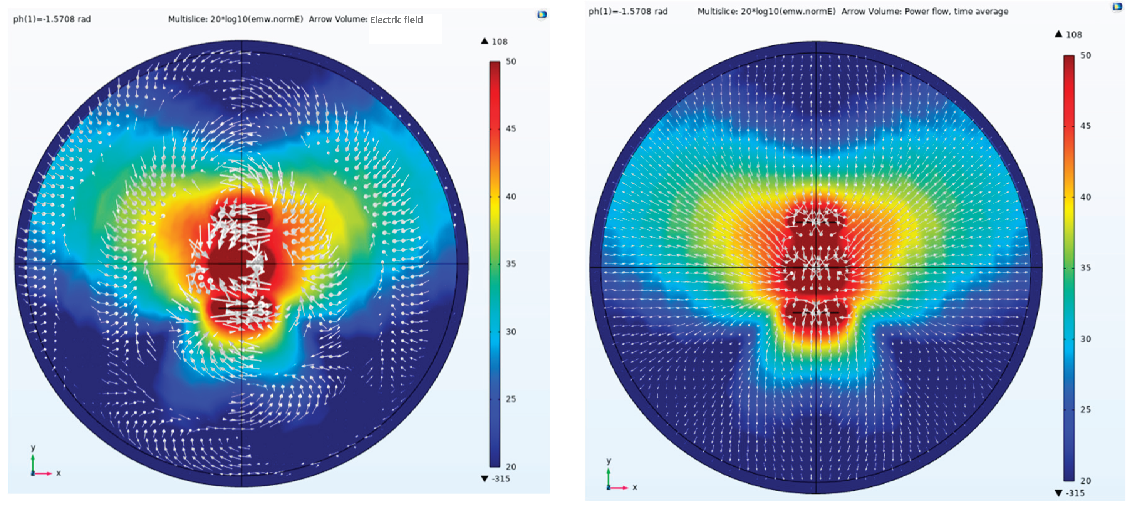
Figure 13.
In the side view of the electric field amplitude, direction and Poynting vector arrow, the three antenna elements are excited by the Taylor synthesis and -1.0472 rad phase difference.
Figure 13.
In the side view of the electric field amplitude, direction and Poynting vector arrow, the three antenna elements are excited by the Taylor synthesis and -1.0472 rad phase difference.
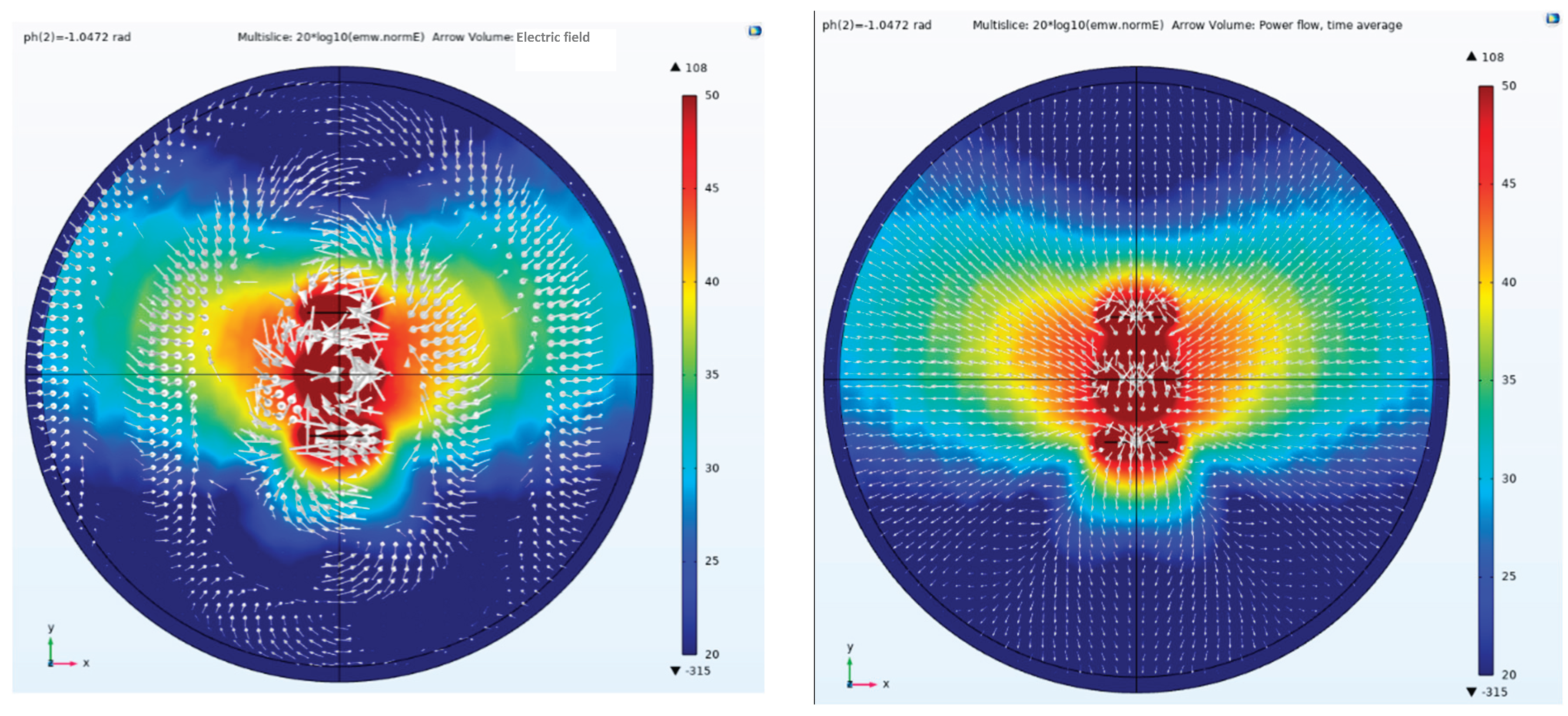
Figure 14.
In the side view of the electric field amplitude, direction and Poynting vector arrow, the three antenna elements are excited by the Taylor synthesis and -0.5236 rad phase difference.
Figure 14.
In the side view of the electric field amplitude, direction and Poynting vector arrow, the three antenna elements are excited by the Taylor synthesis and -0.5236 rad phase difference.
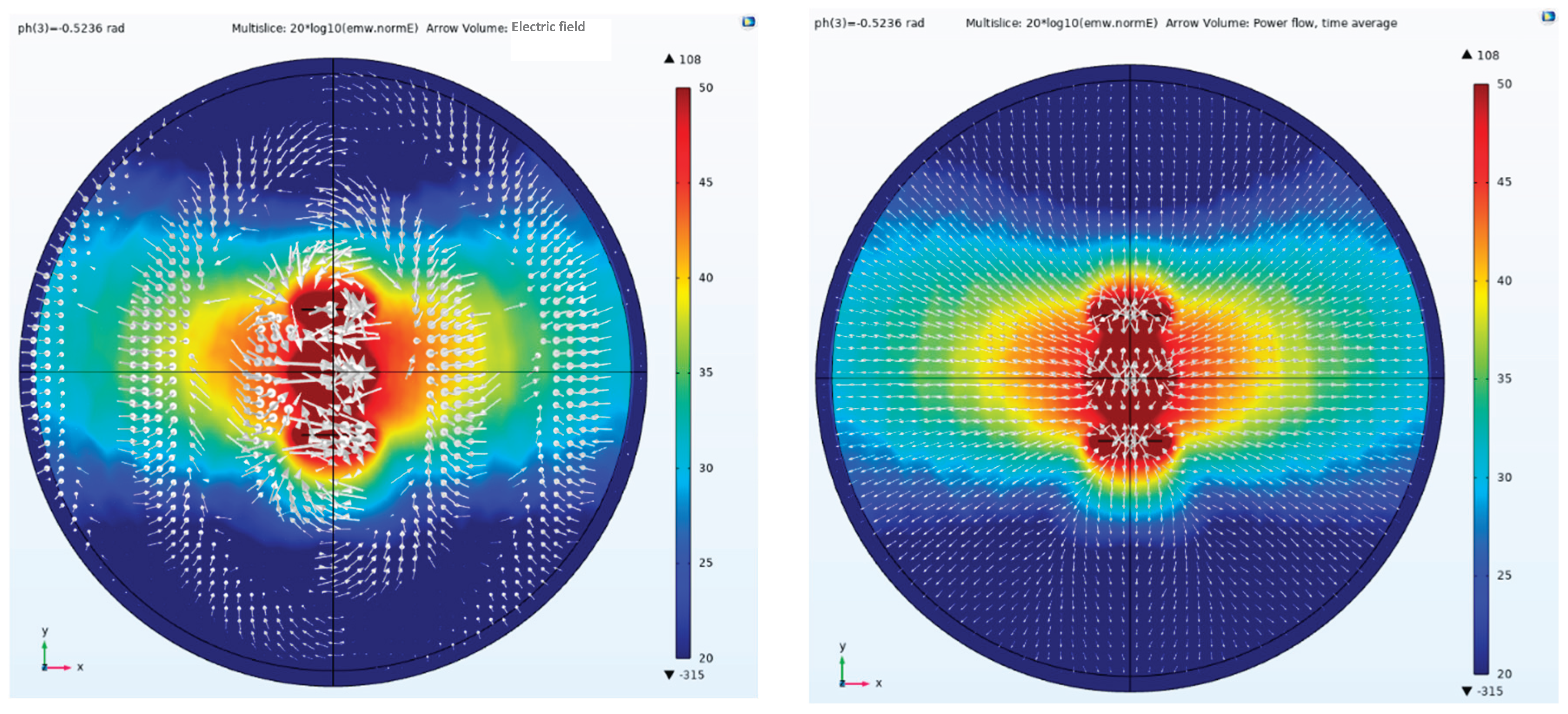
Figure 15.
In the side view of the electric field amplitude, direction and Poynting vector arrow, the three antenna elements are excited by the Taylor synthesis and 0.5236 rad phase difference.
Figure 15.
In the side view of the electric field amplitude, direction and Poynting vector arrow, the three antenna elements are excited by the Taylor synthesis and 0.5236 rad phase difference.
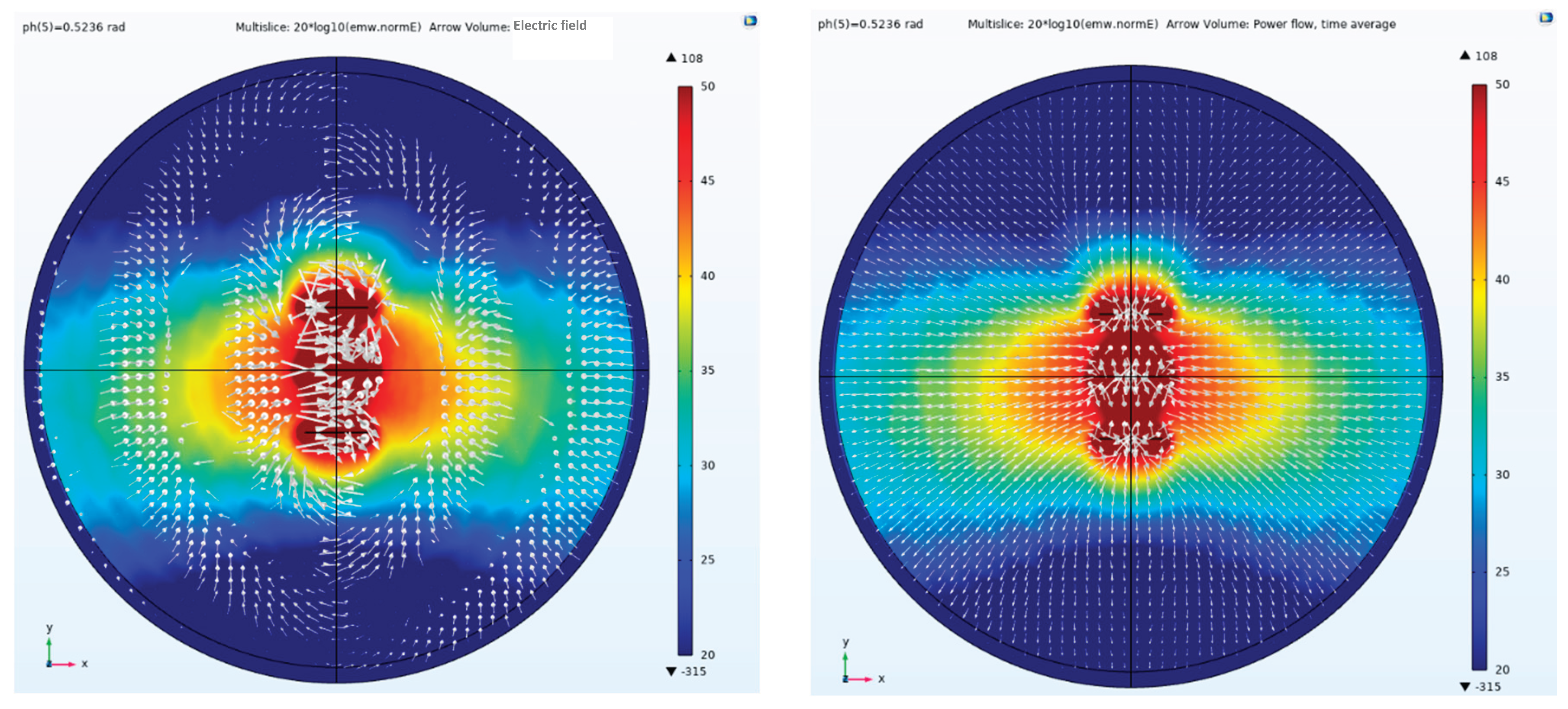
Figure 18.
Pattern of E planes, the three array element antennas are given amplitude Taylor synthesis and different phase excitation. The port phase of array element 1 is 0 rad, and the port phase of array element 2 is changed from -1.5708 to 1.5708 rad every 0.5236 rad. The change of the port phase of array element 3 is twice the change of array element 2.
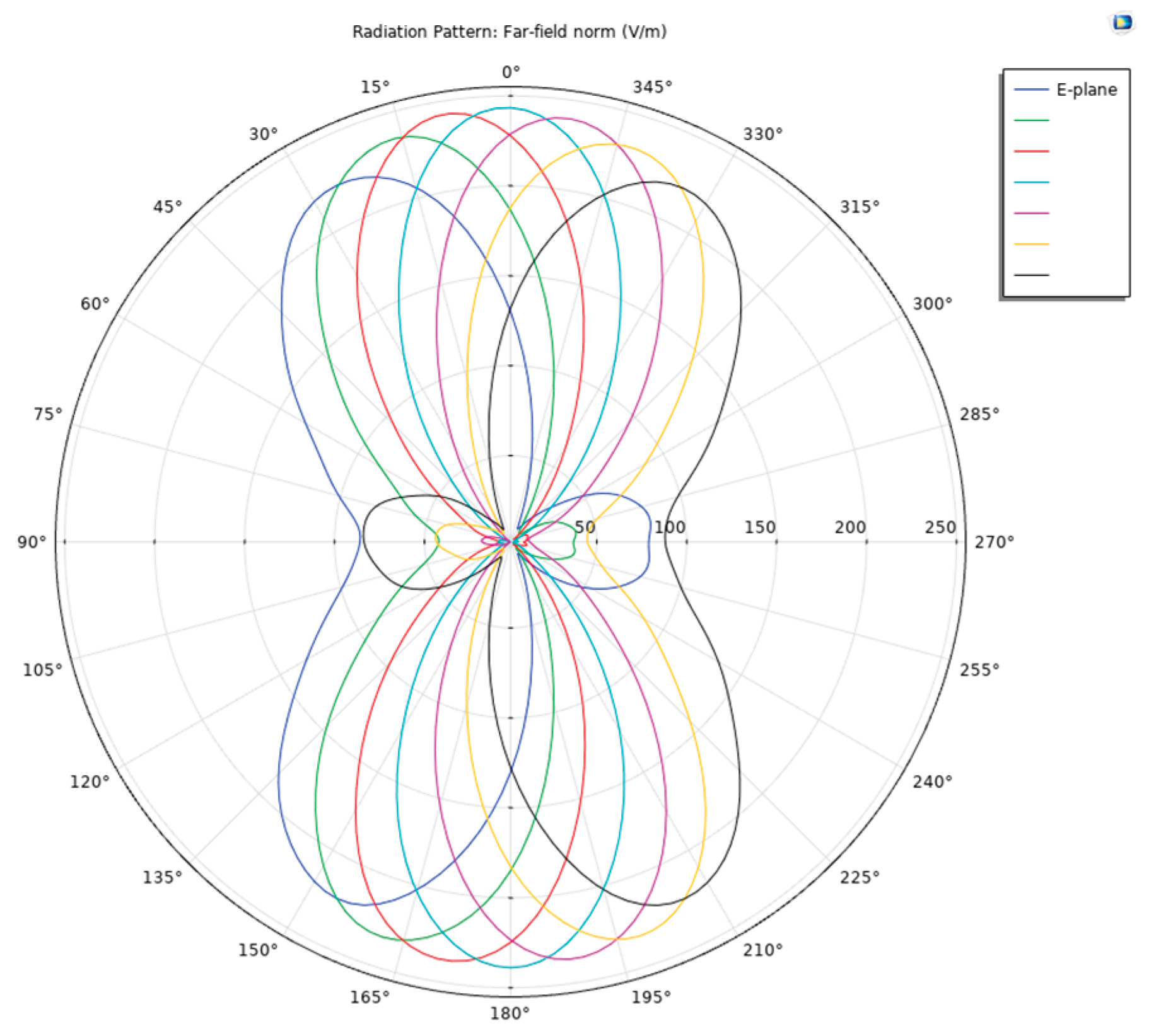
Figure 19.
Pattern of H planes, the three array element antennas are given amplitude Taylor synthesis and different phase excitation. The port phase of array element 1 is 0 rad, and the port phase of array element 2 is changed from -1.5708 to 1.5708 rad every 0.5236 rad. The change of the port phase of array element 3 is twice the change of array element 2.
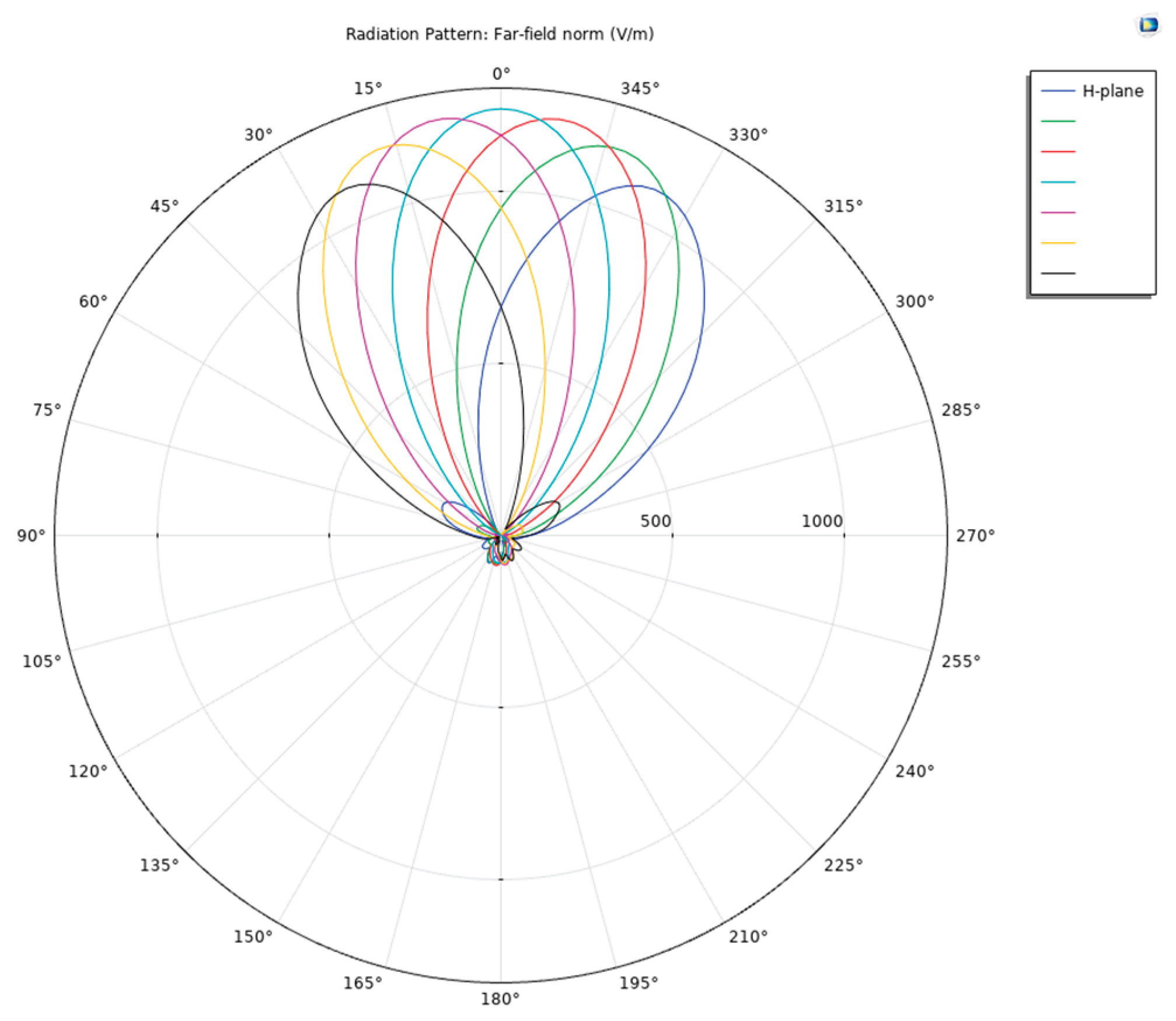
Figure 20.
3D far-field pattern. the left picture shows the situation when ph=-1.5708 rad, the right picture shows the situation when ph=1.5708 rad.
Figure 20.
3D far-field pattern. the left picture shows the situation when ph=-1.5708 rad, the right picture shows the situation when ph=1.5708 rad.
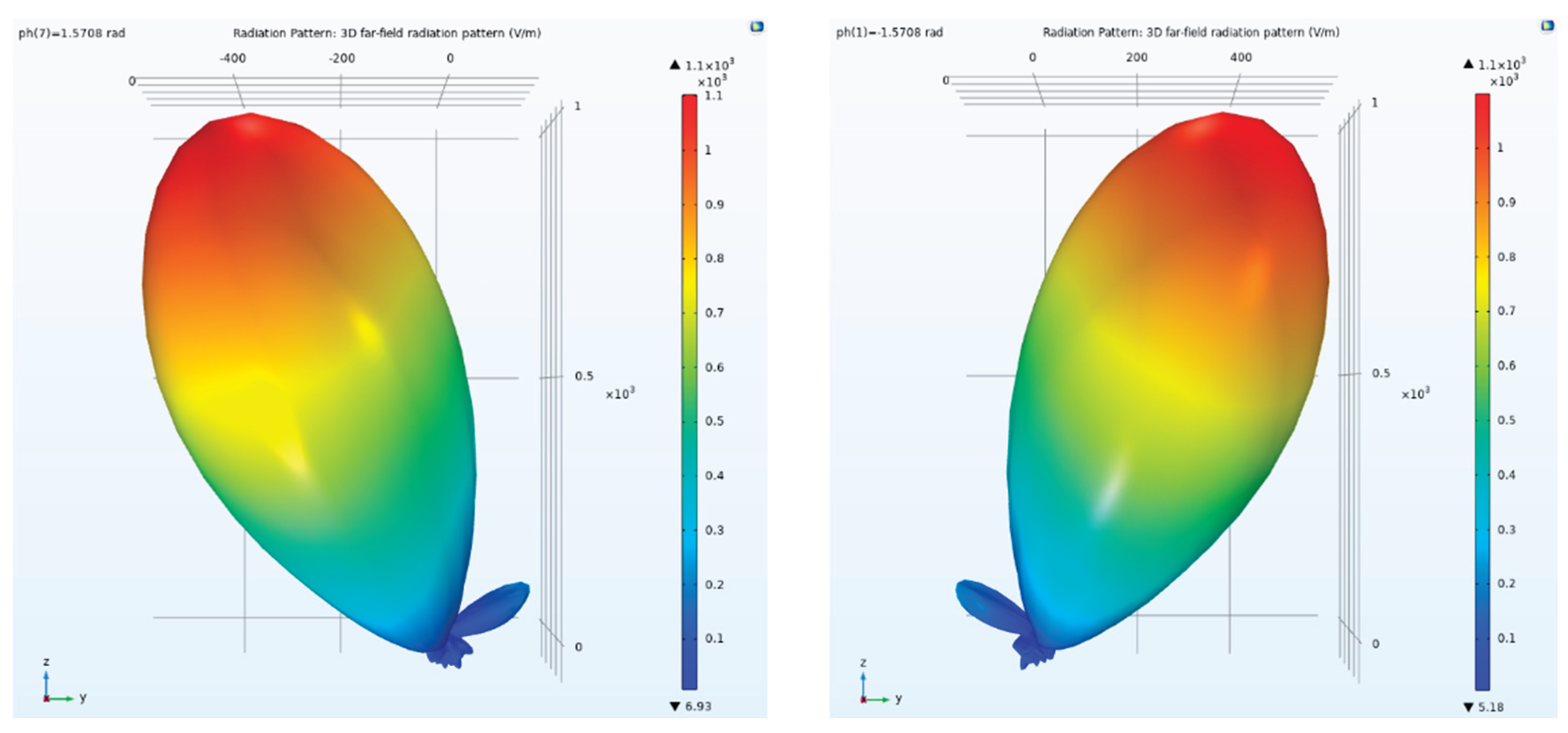
Figure 21.
3D far-field pattern. the picture shows the situation when ph=0 rad.
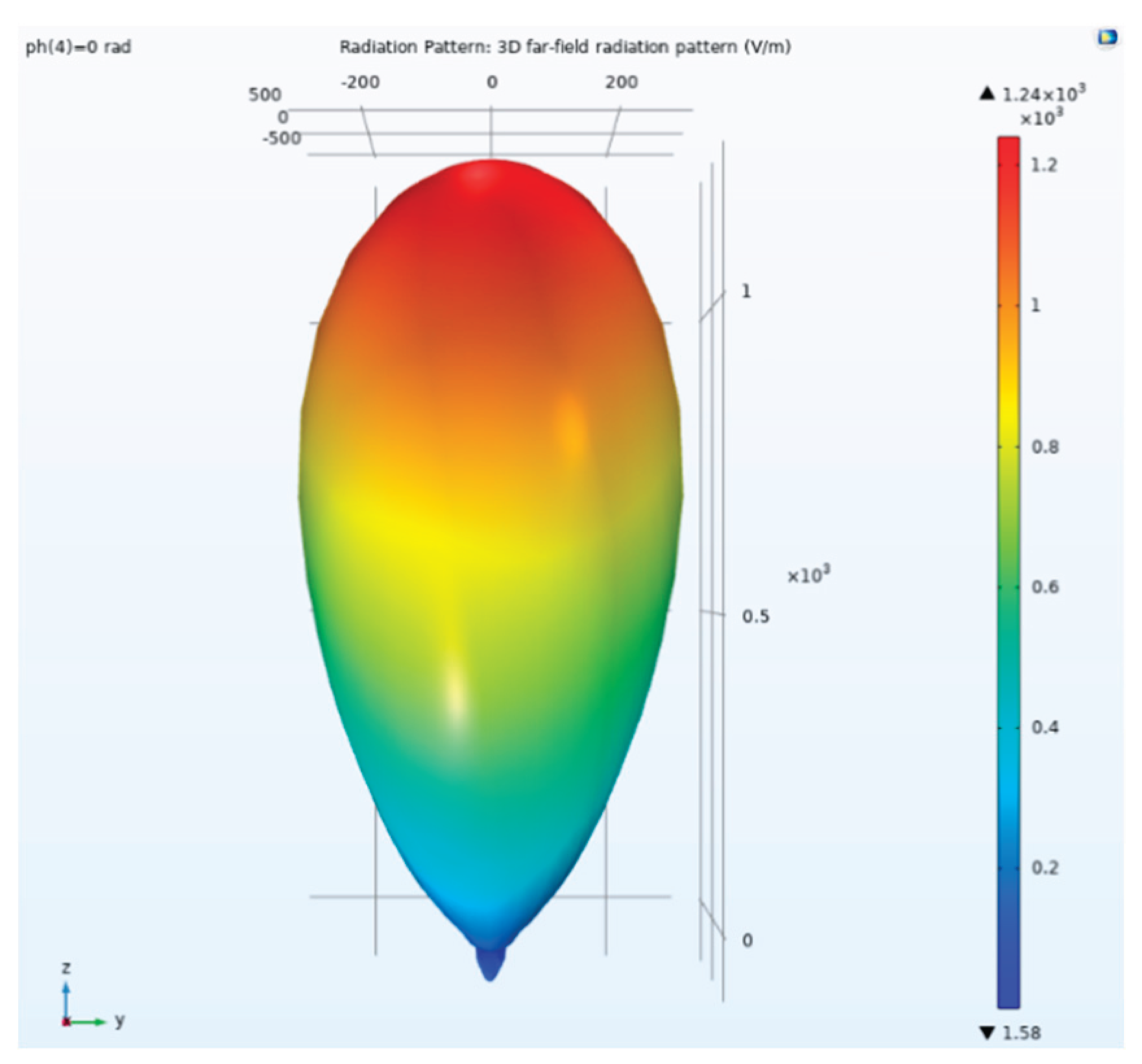
Figure 22.
Numerical simulation of CSAMT adaptive beamforming based on a parallel dipole linear array artificial field source with different ph.
Figure 22.
Numerical simulation of CSAMT adaptive beamforming based on a parallel dipole linear array artificial field source with different ph.
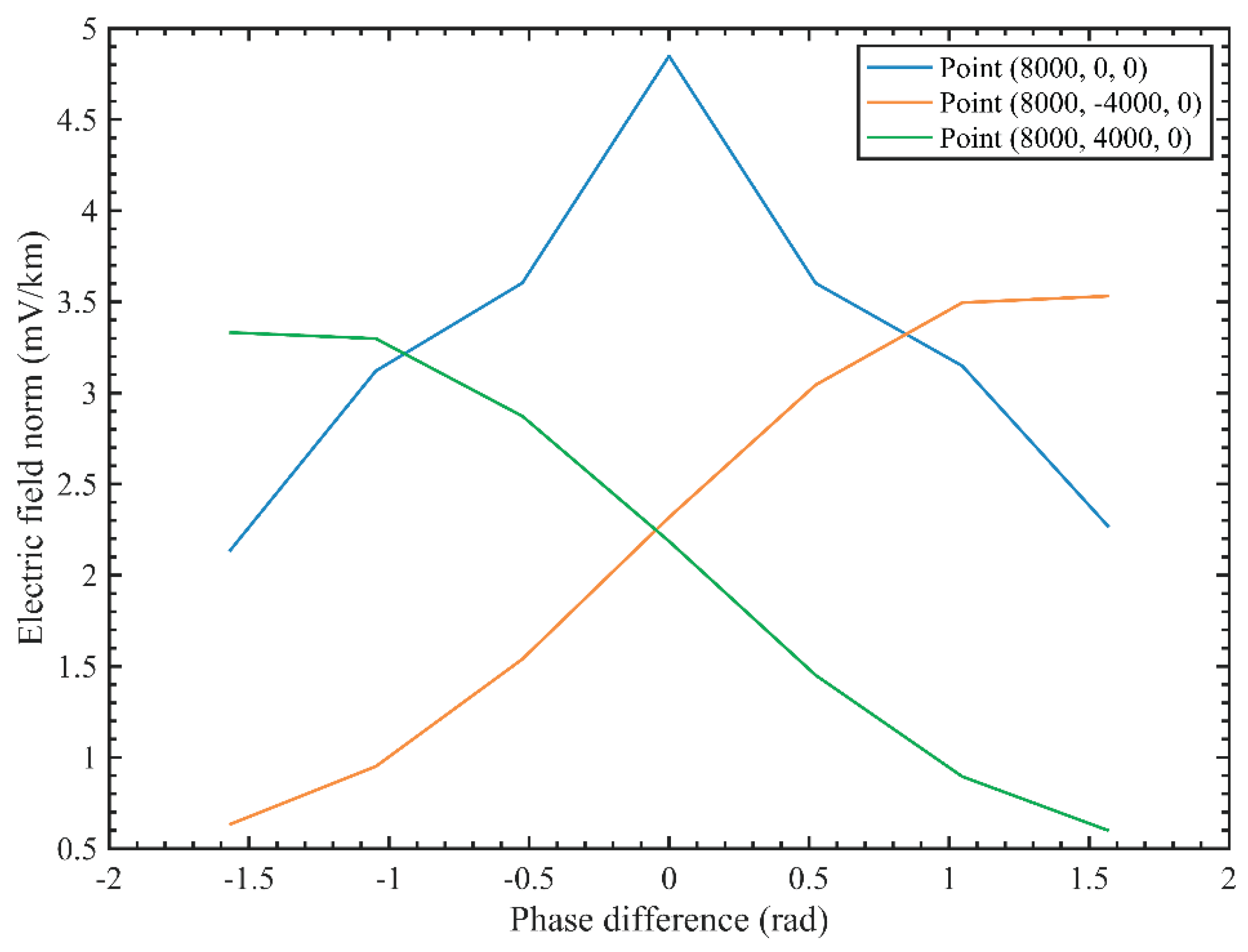
Figure 23.
Coaxial dipole 3×1 antenna array lumped port.
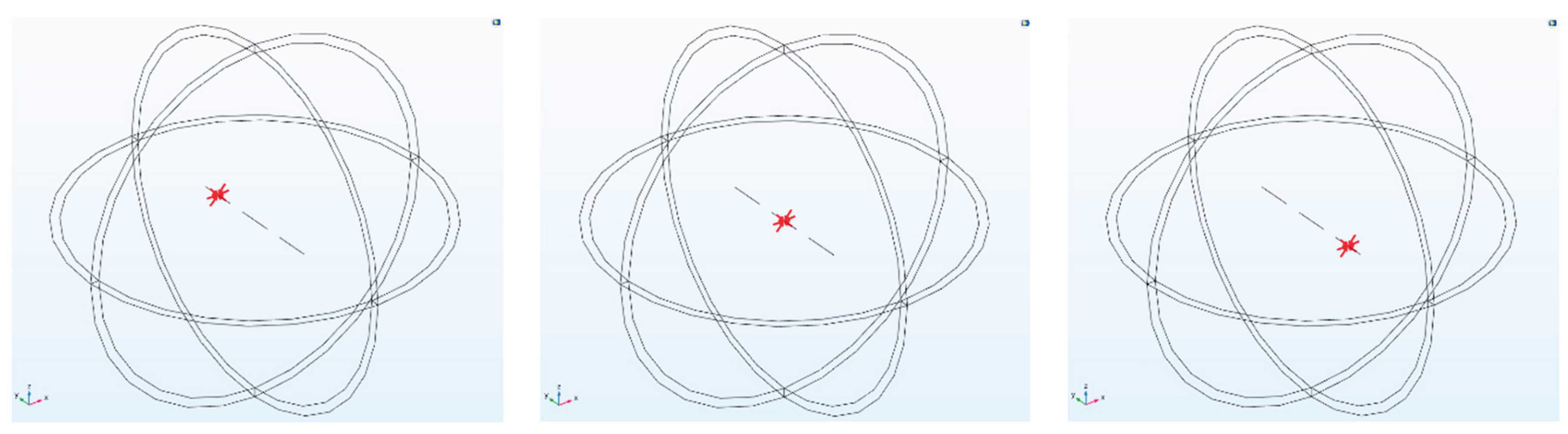
Figure 24.
Side view of electric field amplitude, direction and Poynting vector arrow, array antennas are excited by the same phase (0 rad).
Figure 24.
Side view of electric field amplitude, direction and Poynting vector arrow, array antennas are excited by the same phase (0 rad).
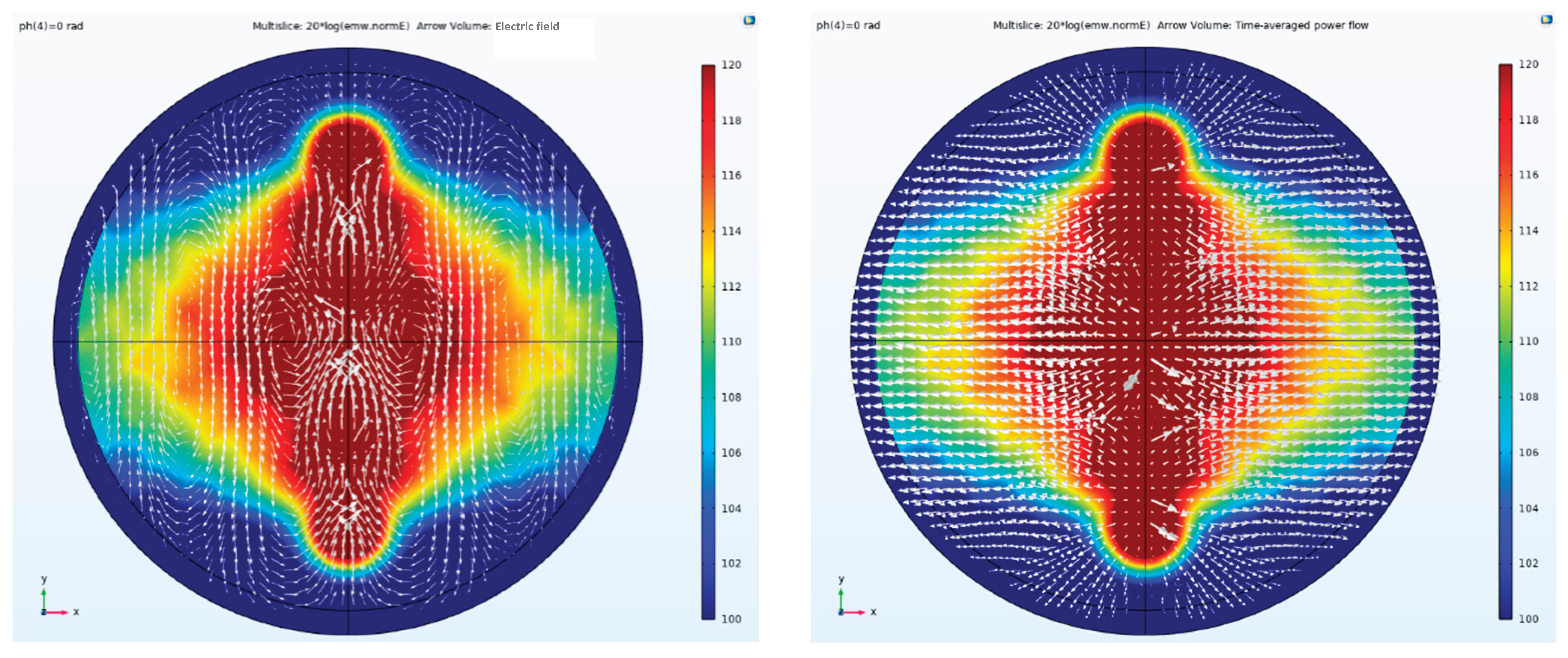
Figure 25.
In the side view of the electric field amplitude, direction and Poynting vector arrow, the array antennas are excited by the Taylor synthesis and -1.5708 rad phase difference.
Figure 25.
In the side view of the electric field amplitude, direction and Poynting vector arrow, the array antennas are excited by the Taylor synthesis and -1.5708 rad phase difference.
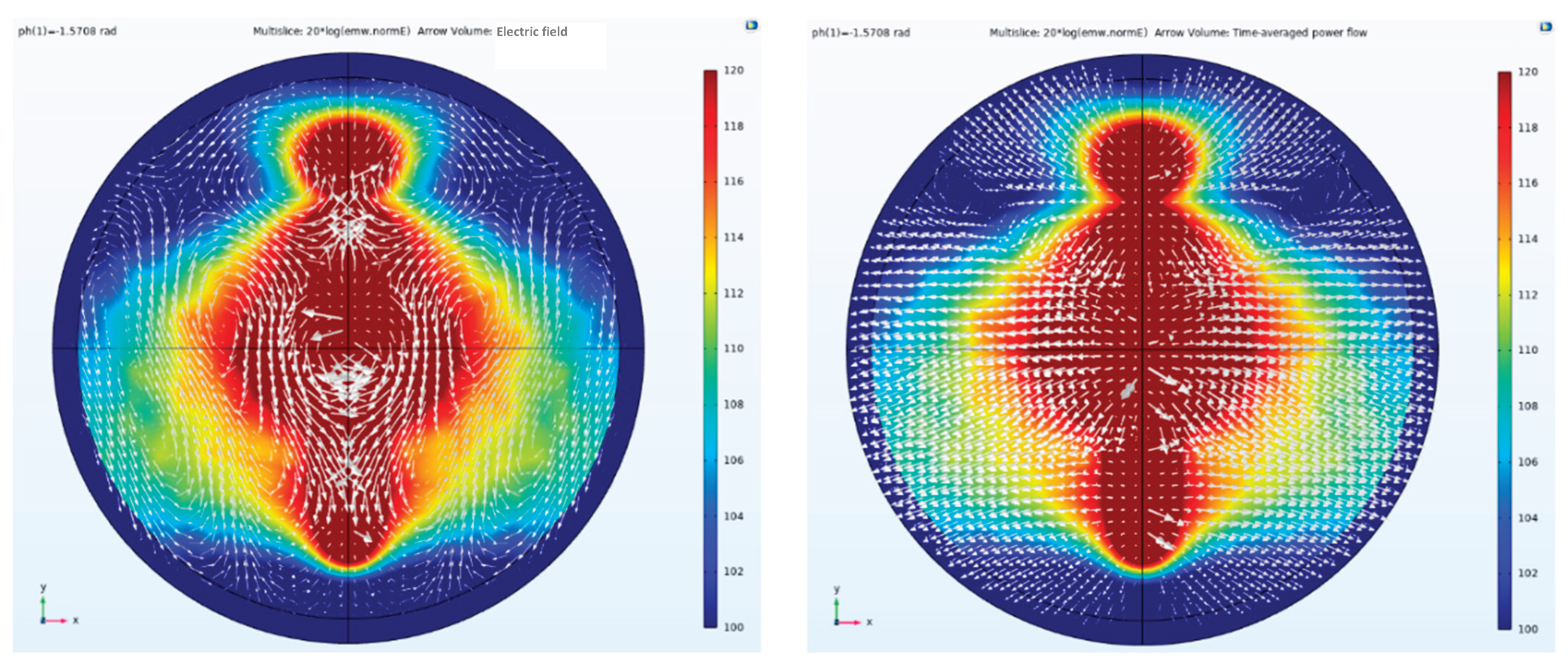
Figure 26.
In the side view of the electric field amplitude, direction and Poynting vector arrow, the array antennas are excited by the Taylor synthesis and -1.0472 rad phase difference.
Figure 26.
In the side view of the electric field amplitude, direction and Poynting vector arrow, the array antennas are excited by the Taylor synthesis and -1.0472 rad phase difference.
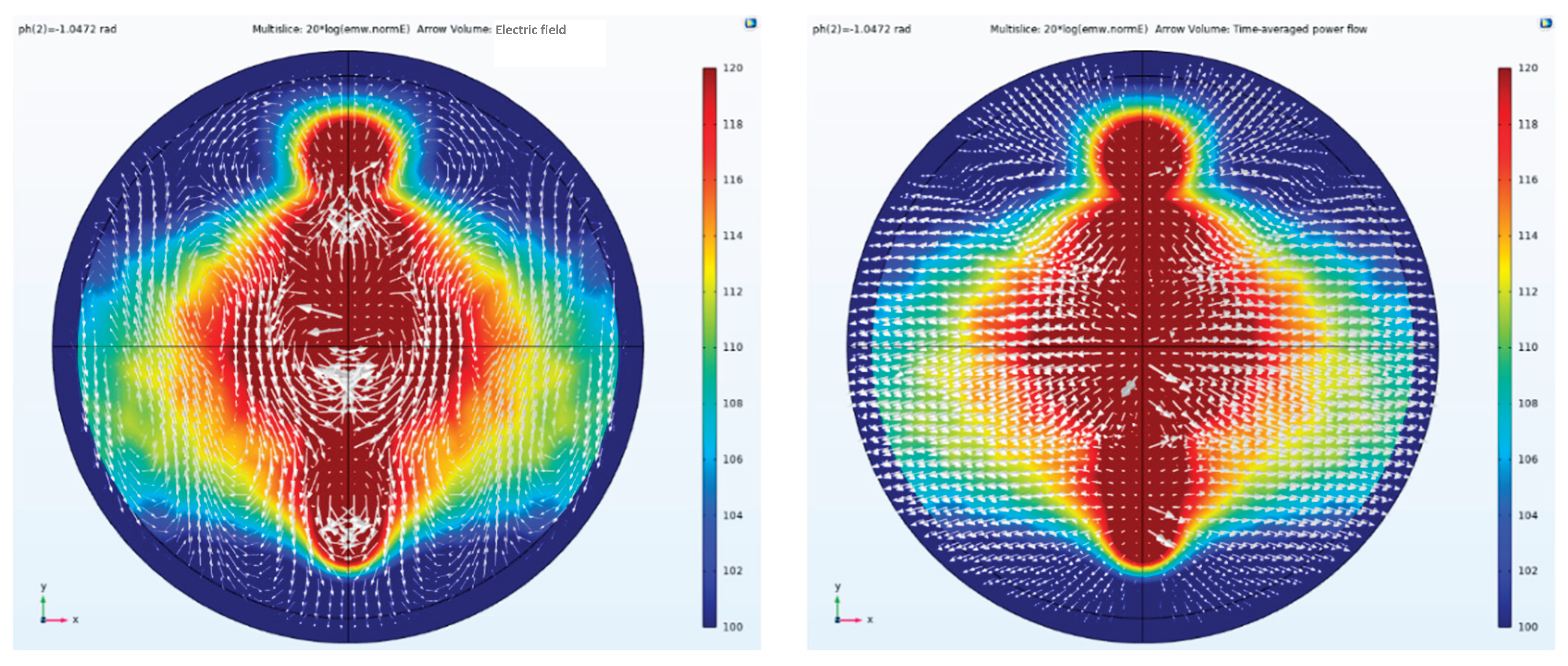
Figure 27.
In the side view of the electric field amplitude, direction and Poynting vector arrow, the array antennas are excited by the Taylor synthesis and -0.5236 rad phase difference.
Figure 27.
In the side view of the electric field amplitude, direction and Poynting vector arrow, the array antennas are excited by the Taylor synthesis and -0.5236 rad phase difference.
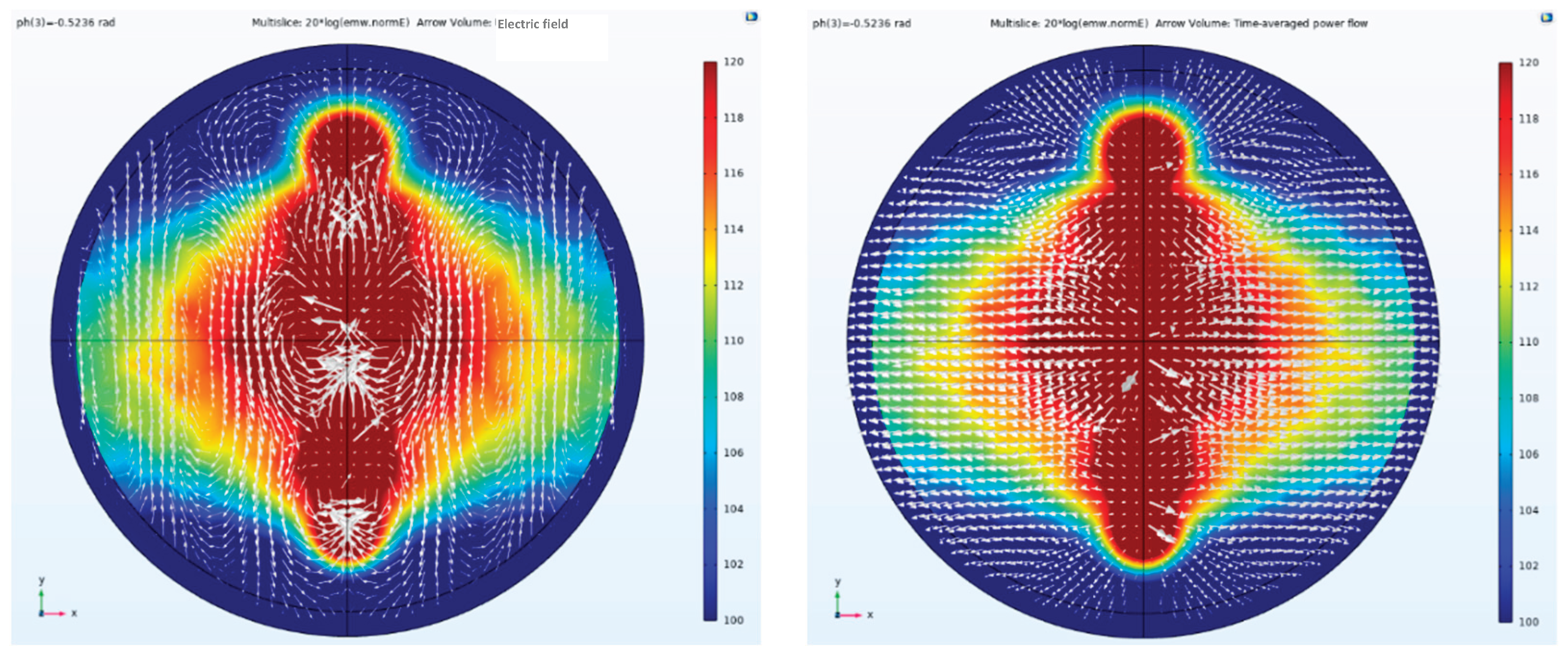
Figure 28.
In the side view of the electric field amplitude, direction and Poynting vector arrow, the array antennas are excited by the Taylor synthesis and 0.5236 rad phase difference.
Figure 28.
In the side view of the electric field amplitude, direction and Poynting vector arrow, the array antennas are excited by the Taylor synthesis and 0.5236 rad phase difference.
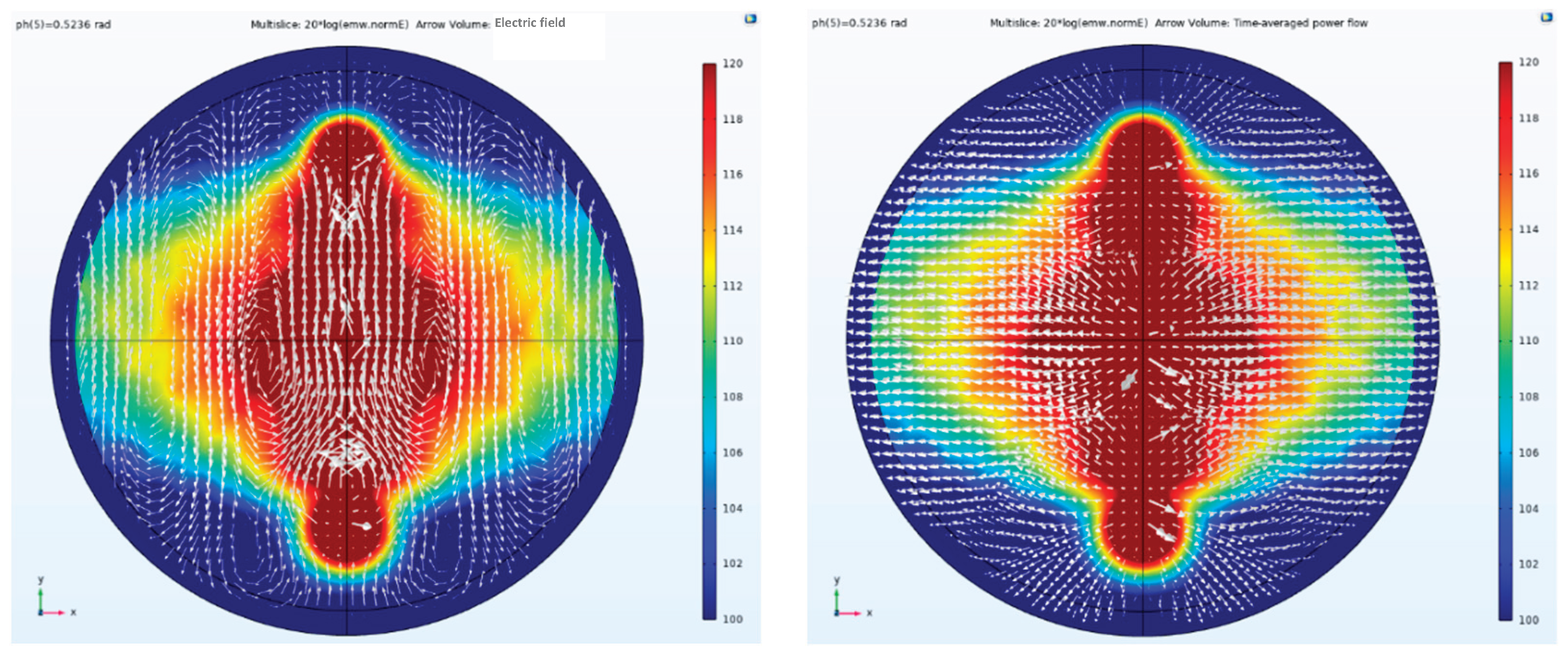
Figure 29.
In the side view of the electric field amplitude, direction and Poynting vector arrow, the array antennas are excited by the Taylor synthesis and 1.0472 rad phase difference.
Figure 29.
In the side view of the electric field amplitude, direction and Poynting vector arrow, the array antennas are excited by the Taylor synthesis and 1.0472 rad phase difference.
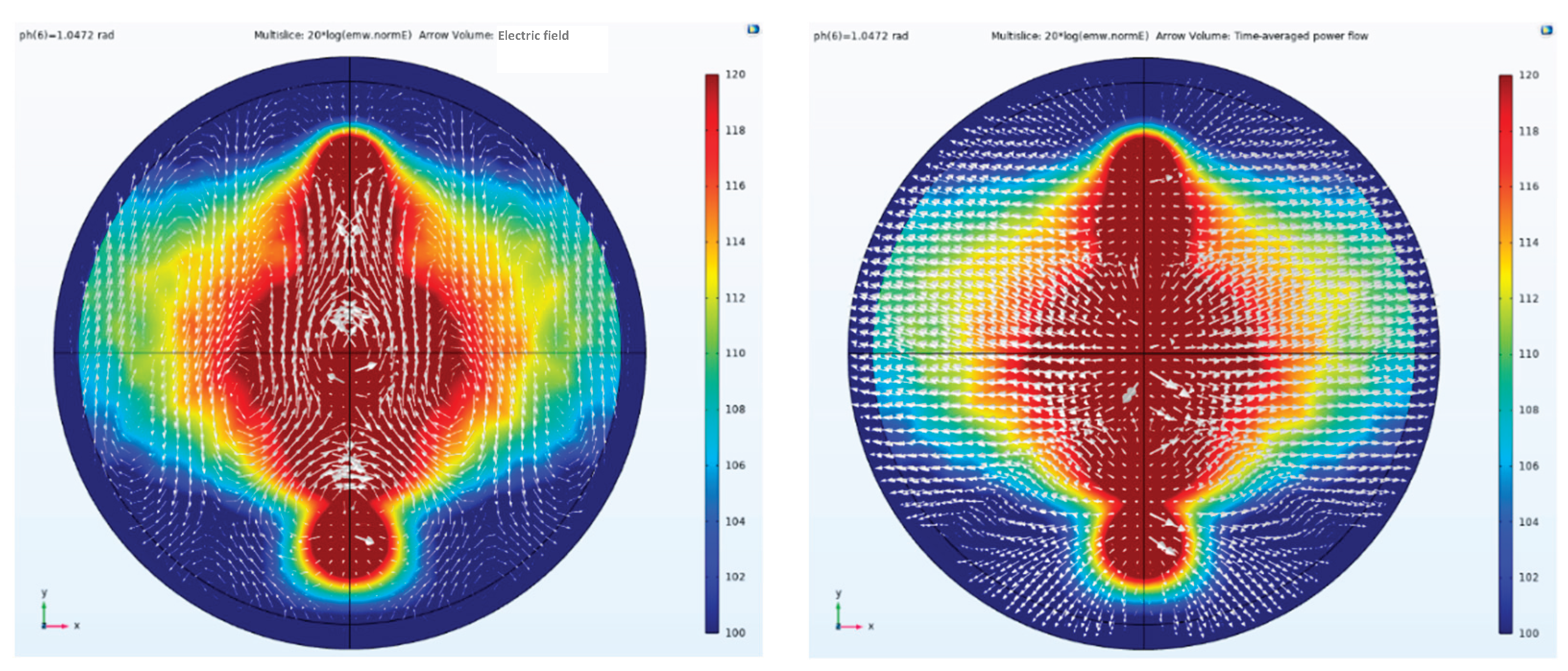
Figure 30.
In the side view of the electric field amplitude, direction and Poynting vector arrow, the array antennas are excited by the Taylor synthesis and 1.5708 rad phase difference.
Figure 30.
In the side view of the electric field amplitude, direction and Poynting vector arrow, the array antennas are excited by the Taylor synthesis and 1.5708 rad phase difference.
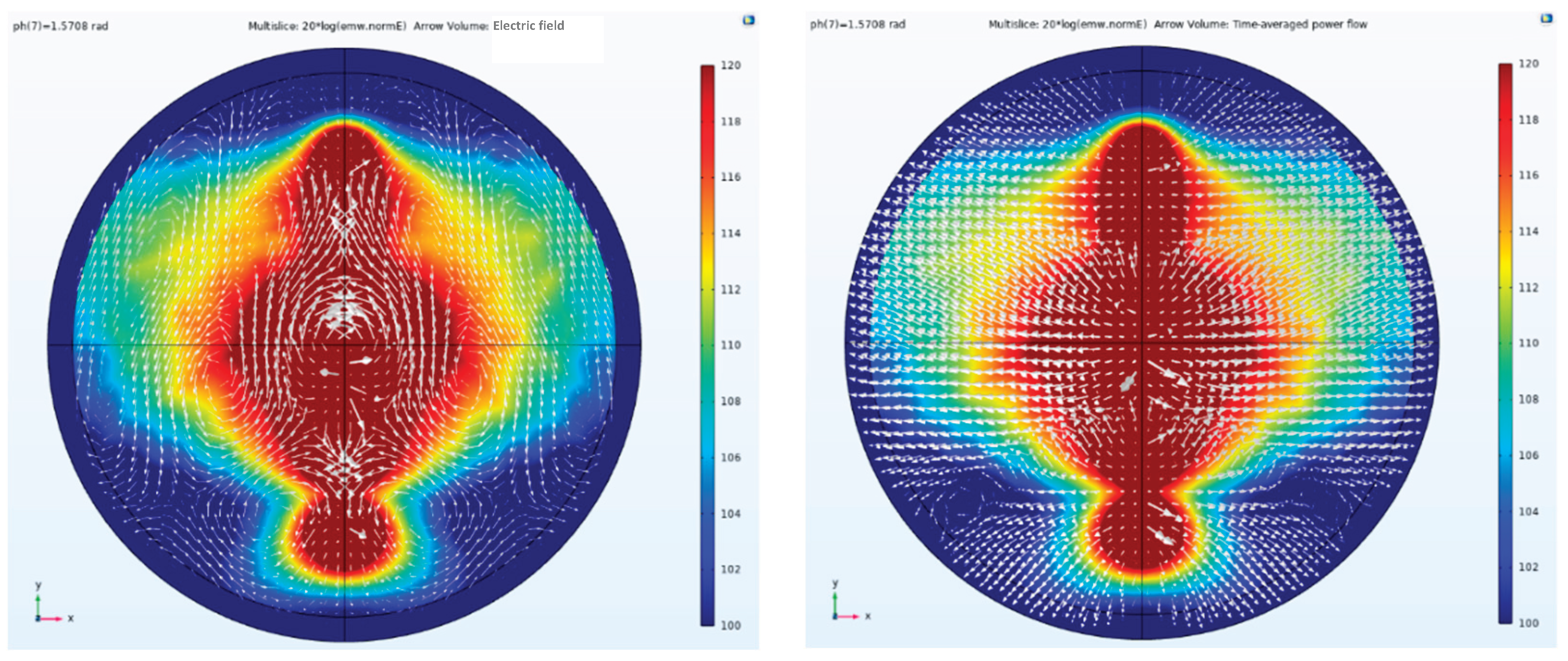
Figure 31.
Pattern of E planes, the three array antennas are given amplitude Taylor synthesis and different phase excitation. The port phase of array antenna 1 is 0 rad, and the port phase of array antenna 2 is changed from -1.5708 to 1.5708 rad every 0.5236 rad. The change of the port phase of array antenna 3 is twice the change of array antenna 2.
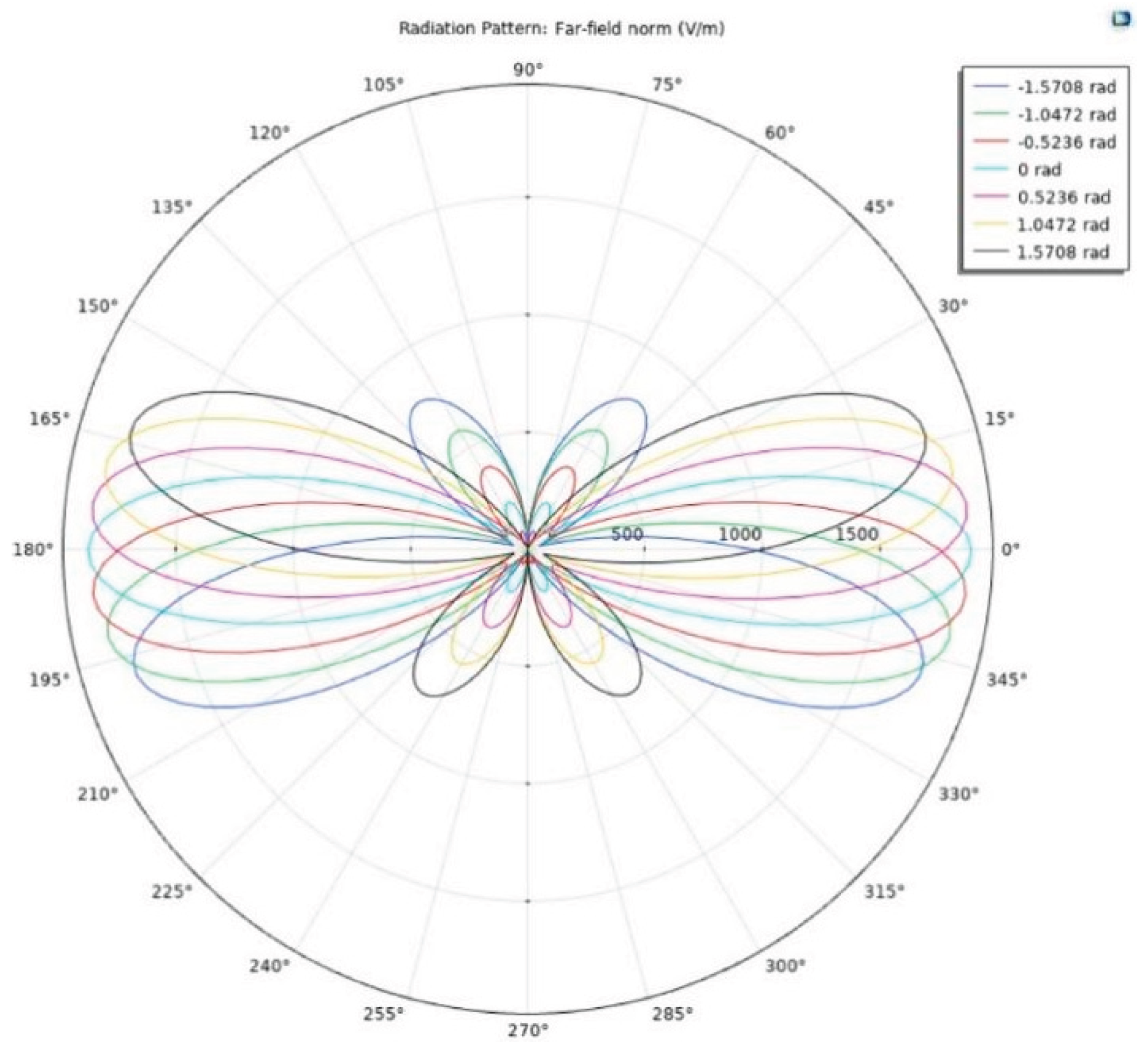
Figure 32.
Numerical simulation of CSAMT adaptive beamforming based on coaxial dipole linear array artificial field source with different ph.
Figure 32.
Numerical simulation of CSAMT adaptive beamforming based on coaxial dipole linear array artificial field source with different ph.
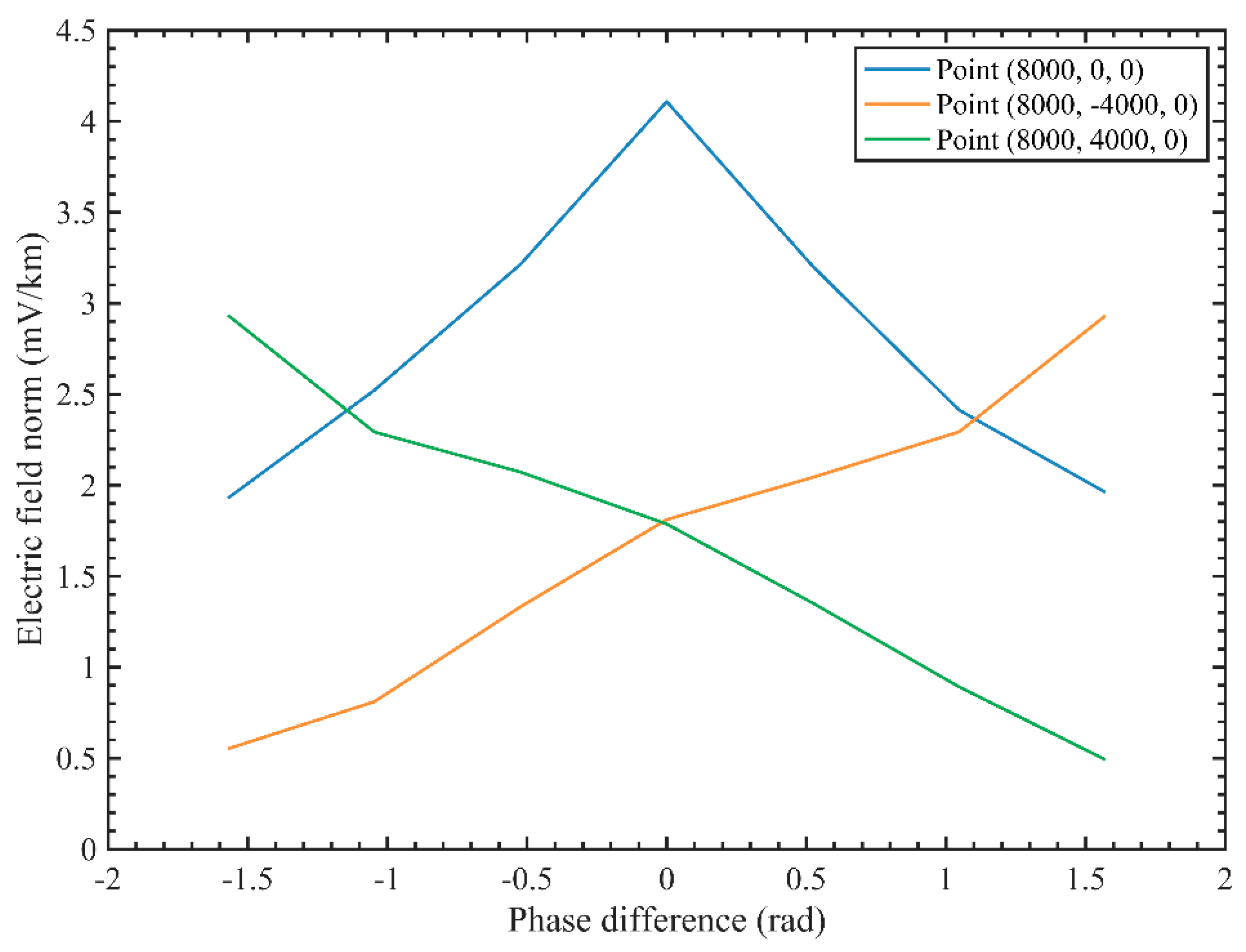
Figure 33.
GPS time synchronization diagram.
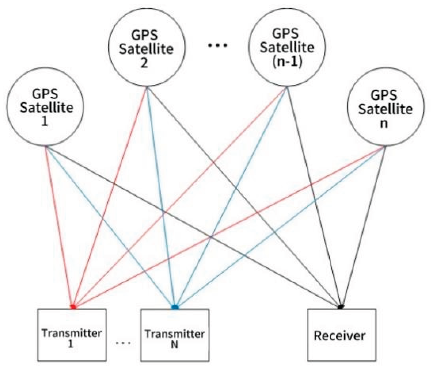
Figure 34.
The block diagram of GPS time synchronization.
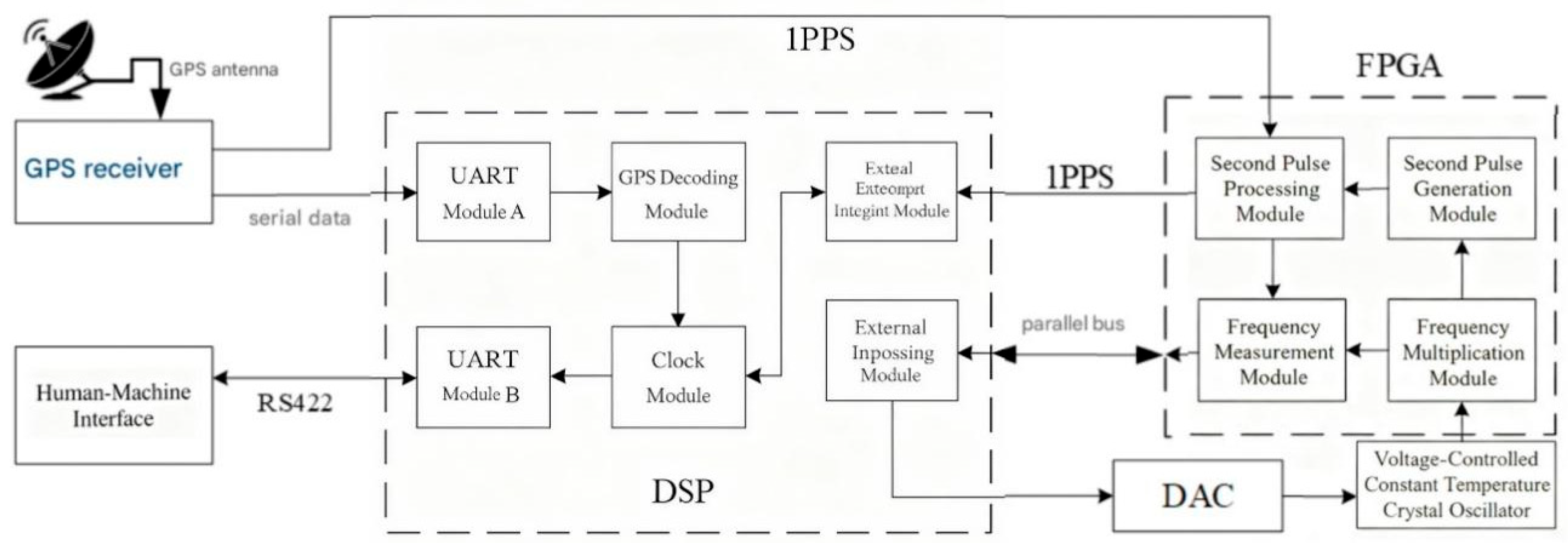
Figure 35.
Principles of DDS table lookup method.
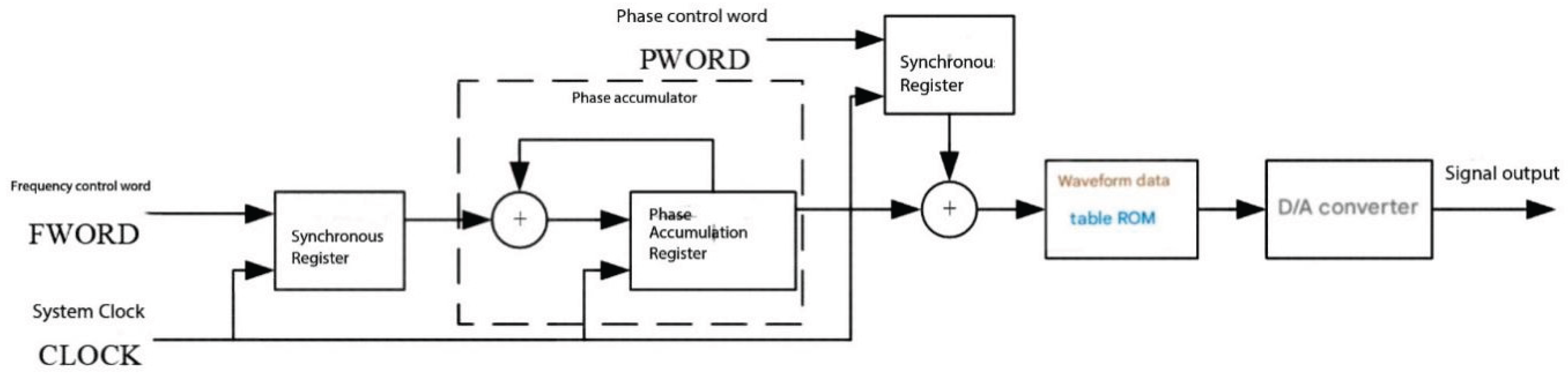
Figure 36.
Comparison of triangle carrier and sine wave.
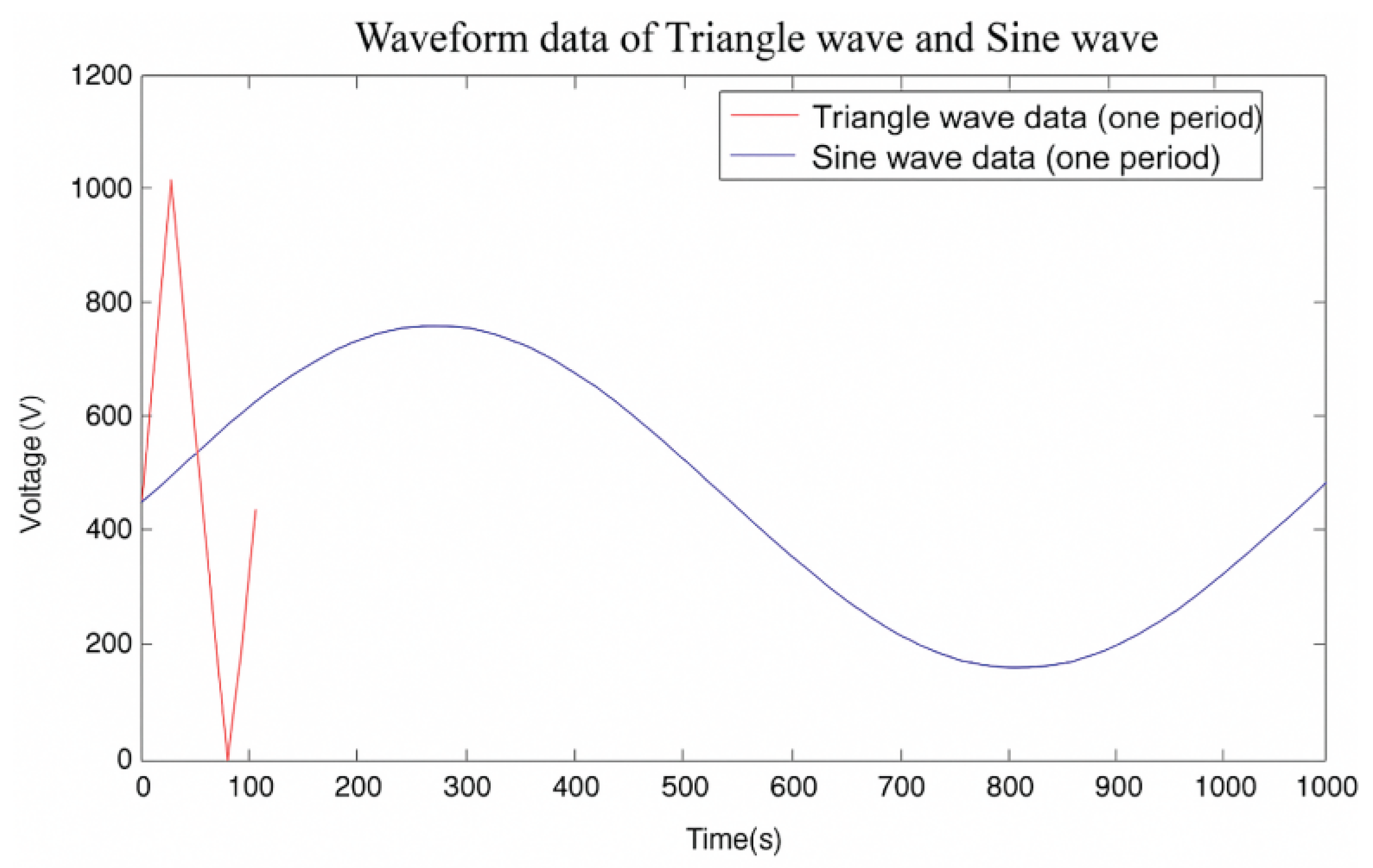
Figure 37.
FPGA implementation of DDS table lookup method.
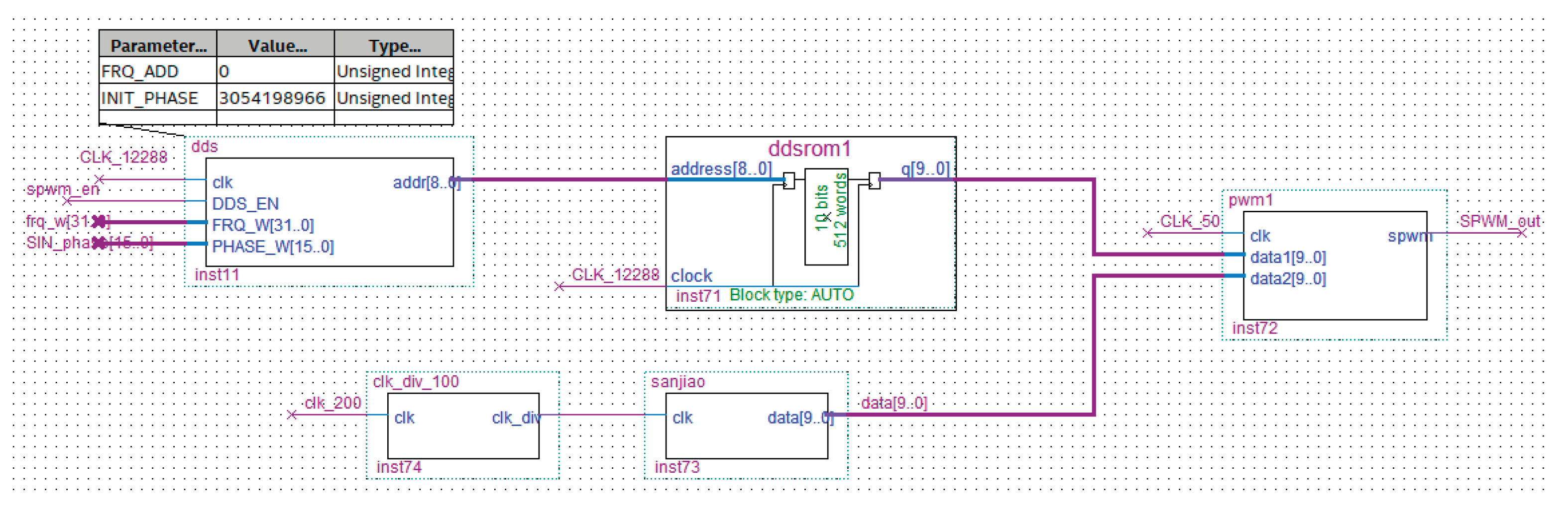
Figure 38.
Phase control system.
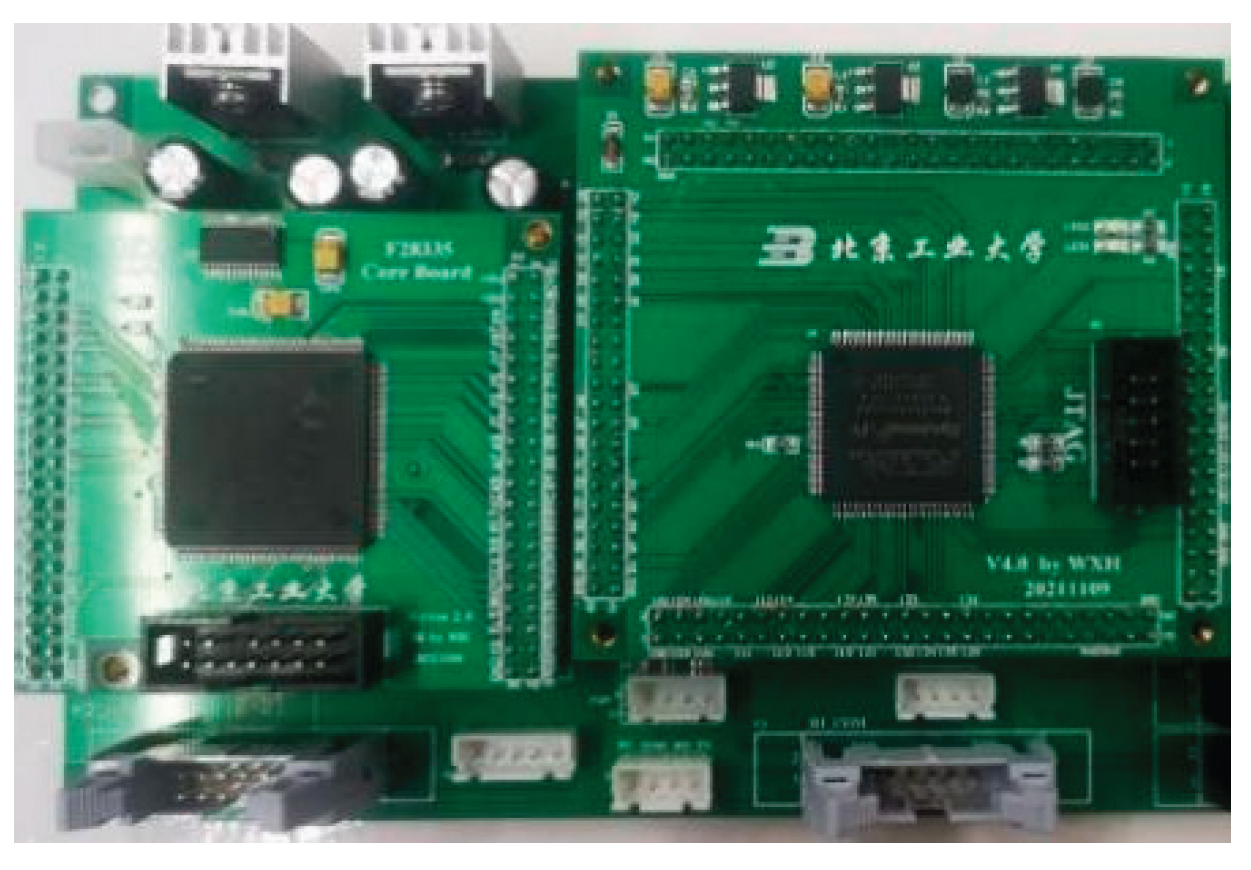
Figure 39.
Adaptive beamforming measurement of parallel vibrator linear array artificial field source.
Figure 39.
Adaptive beamforming measurement of parallel vibrator linear array artificial field source.
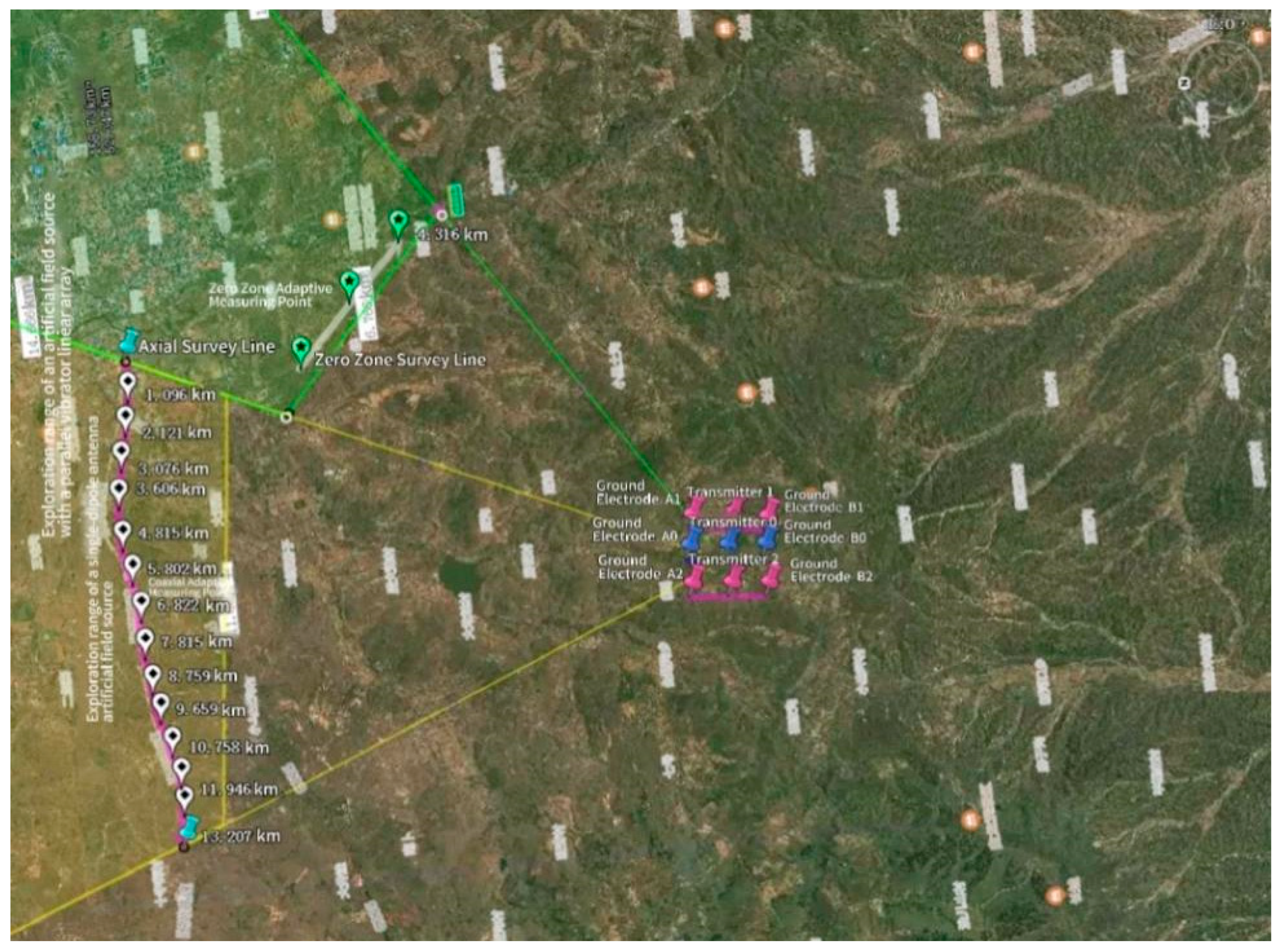
Figure 40.
Coaxial adaptive beamforming measurement of parallel vibrator linear array artificial field source (at the coaxial adaptive measuring point).
Figure 40.
Coaxial adaptive beamforming measurement of parallel vibrator linear array artificial field source (at the coaxial adaptive measuring point).
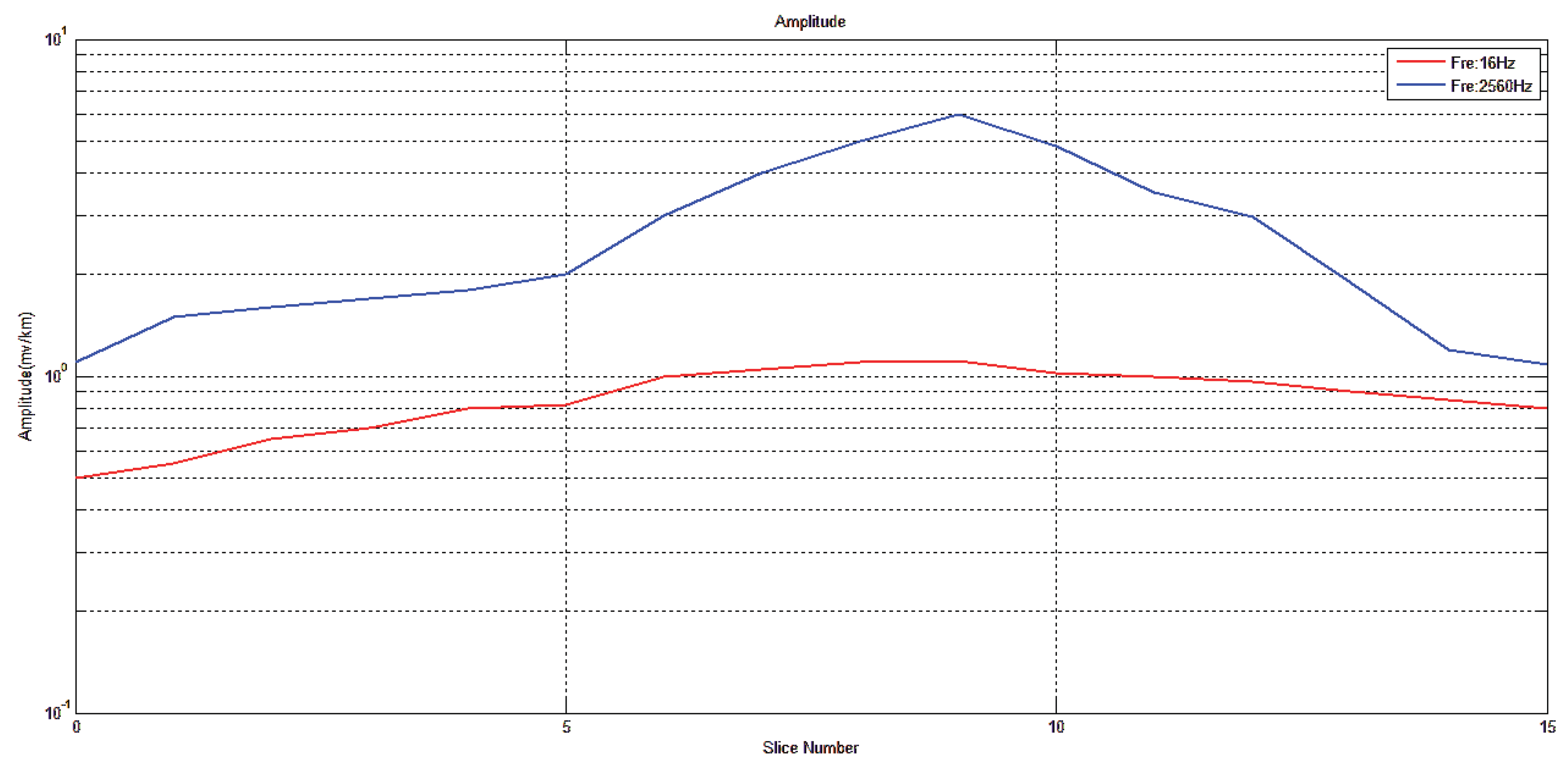
Figure 41.
Zero-zone adaptive beamforming measurement of parallel vibrator linear array artificial field source (at the zero-zone adaptive measuring point ).
Figure 41.
Zero-zone adaptive beamforming measurement of parallel vibrator linear array artificial field source (at the zero-zone adaptive measuring point ).
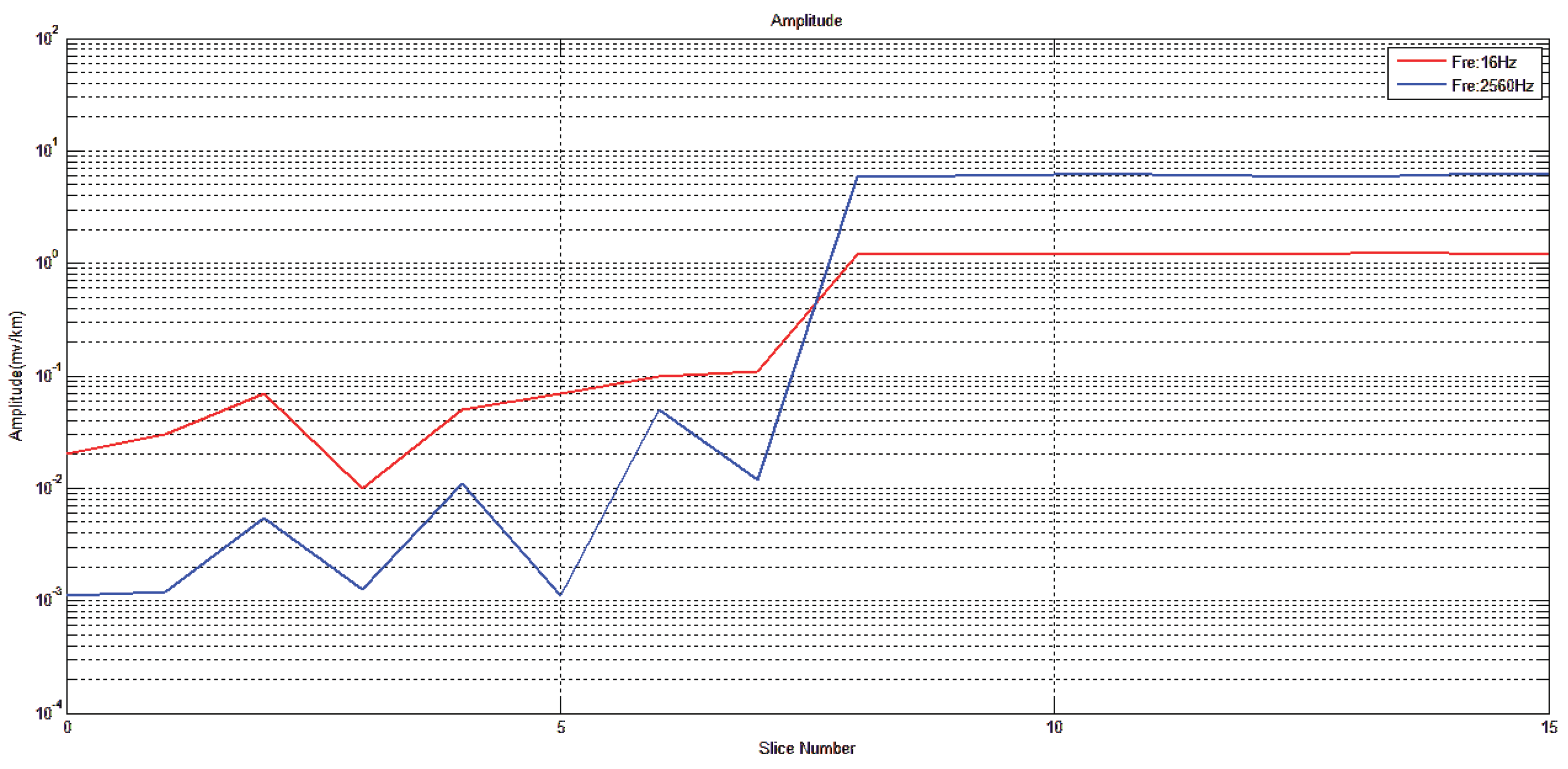
Figure 42.
Adaptive beamforming measurement of coaxial vibrator linear array artificial source.
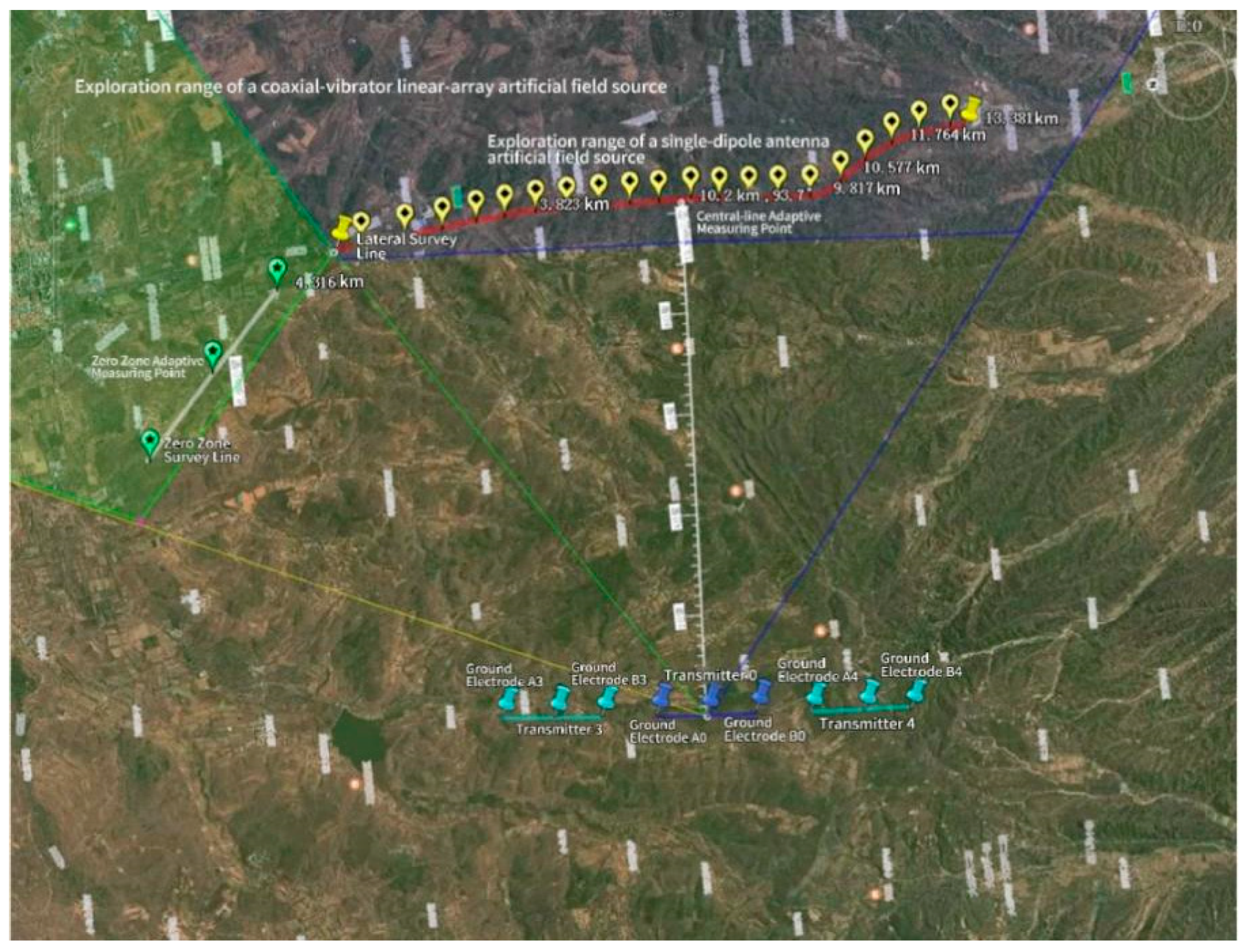
Figure 43.
Side beamforming measurement of coaxial vibrator linear array artificial field source (at the central measuring point).
Figure 43.
Side beamforming measurement of coaxial vibrator linear array artificial field source (at the central measuring point).
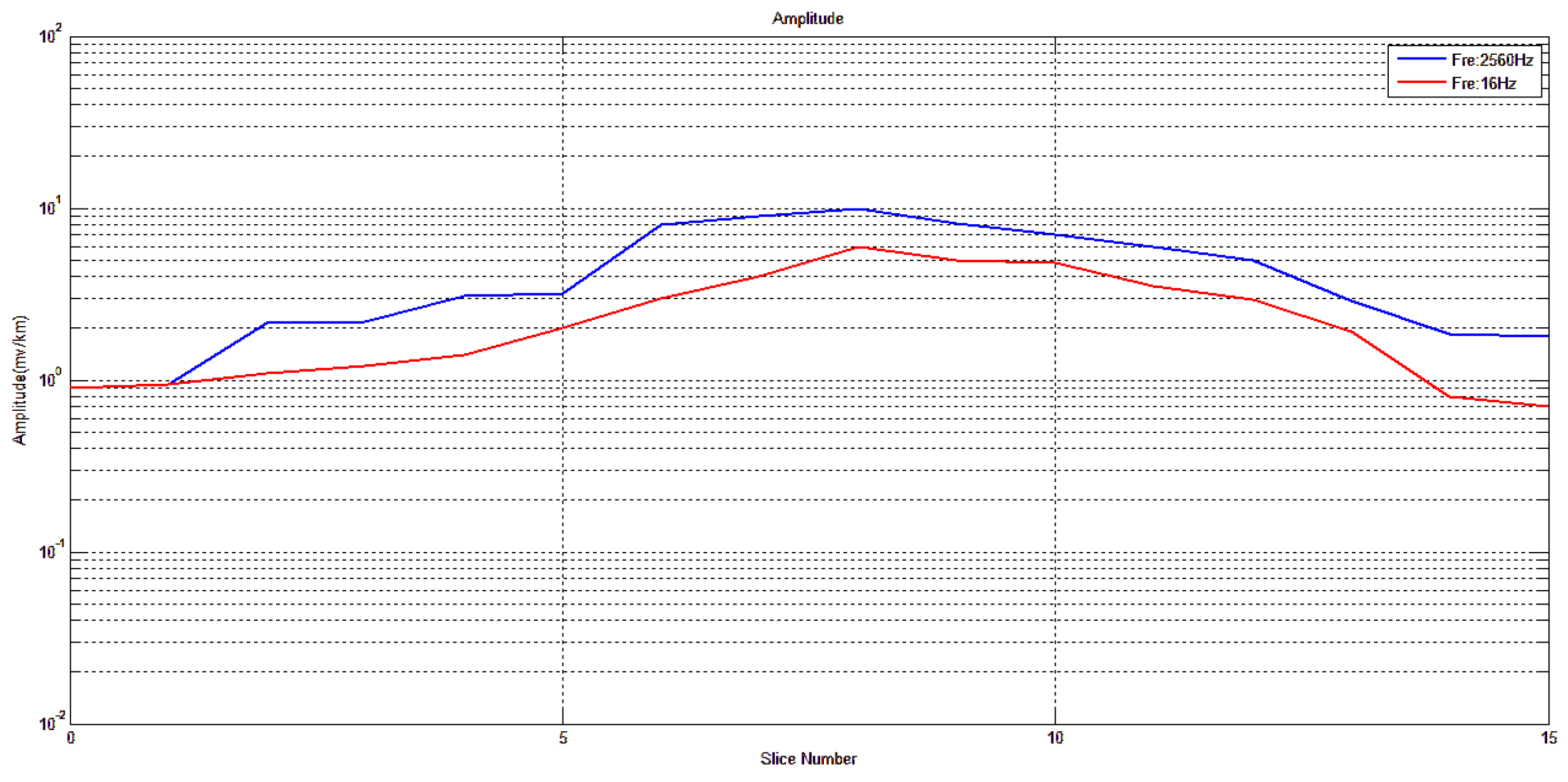
Figure 44.
Zero-zone beamforming measurement of coaxial vibrator linear array artificial field source (at the zero-zone measuring point).
Figure 44.
Zero-zone beamforming measurement of coaxial vibrator linear array artificial field source (at the zero-zone measuring point).
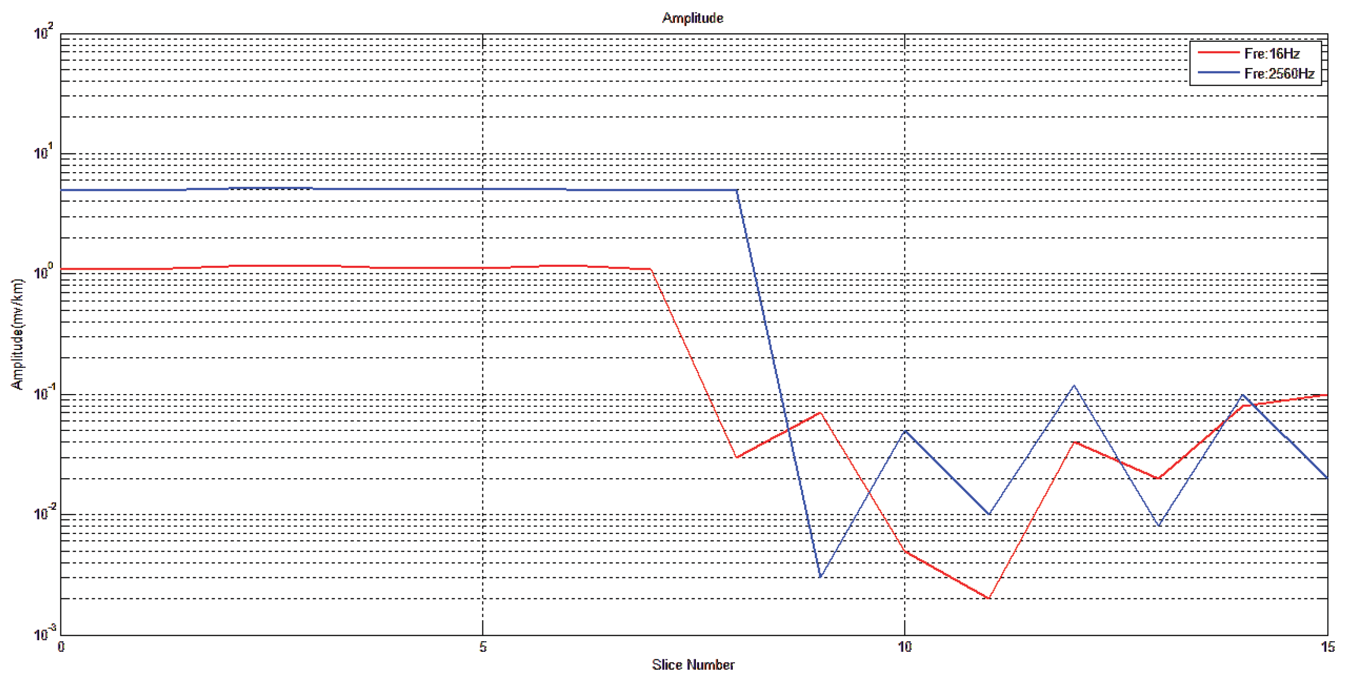

Table 1.
Arithmetic Pd for the different lumped ports, identified by their lumped port name.
| Arithmetic Phase Difference | Lumped Ports of a Parallel Dipole Linear Array |
|---|---|
| 0 [rad] | Port1 |
| ph range(-1.5708, 0.5236, 1.5708 [rad]) | Port2 |
| 2*ph [rad] | Port3 |
Table 2.
Electric field values and F/B with different ph.
| ph (rad) | Electric field value (mV/km), at Point (0, 8000, 0) |
Electric field value (mV/km), at Point (0, -8000, 0) |
F/B (dB) |
|---|---|---|---|
| -1.5708 | 18.67×10⁻⁴ | 8.2892×10⁻⁴ | 3.52 (Forward) |
| -1.0472 | 16.366×10⁻⁴ | 8.6533×10⁻⁴ | 2.76 (Forward) |
| -0.5236 | 14.658×10⁻⁴ | 9.3276×10⁻⁴ | 1.96 (Forward) |
| 0 | 10.276×10⁻⁴ | 10.69×10⁻⁴ | 0.17 (Forward) |
| 0.5236 | 9.0404×10⁻⁴ | 14.156×10⁻⁴ | 1.94 (Backward) |
| 1.0472 | 8.4362×10⁻⁴ | 16.886×10⁻⁴ | 3.01 (Backward) |
| 1.5708 | 8.1602×10⁻⁴ | 18.189×10⁻⁴ | 3.48 (Backward) |
Table 3.
Numerical simulation of CSAMT adaptive beamforming based on parallel dipole linear array artificial field source with different ph.
Table 3.
Numerical simulation of CSAMT adaptive beamforming based on parallel dipole linear array artificial field source with different ph.
| ph (rad) | Electric field value (mV/km), at Point (8000, 0, 0) |
Electric field value (mV/km), at Point (8000, -4000, 0) |
Electric field value (mV/km), at Point (8000, 4000, 0) |
|---|---|---|---|
| -1.5708 | 2.1298 | 0.6312 | 3.3316 |
| -1.0472 | 3.1206 | 0.9508 | 3.2979 |
| -0.5236 | 3.6039 | 1.5398 | 2.8721 |
| 0 | 4.8484 | 2.3173 | 2.1860 |
| 0.5236 | 3.6021 | 3.0439 | 1.4511 |
| 1.0472 | 3.1479 | 3.4953 | 0.8949 |
| 1.5708 | 2.2635 | 3.5314 | 0.5979 |
Table 4.
Arithmetic Pd for the different lumped ports, identified by their lumped port name.
| Arithmetic Phase Difference | Lumped Ports of a Coaxial Dipole Linear Array |
|---|---|
| 0 [rad] | Port1 |
| ph range(-1.5708, 0.5236, 1.5708 [rad]) | Port2 |
| 2*ph [rad] | Port3 |
Table 5.
Numerical simulation of CSAMT adaptive beamforming based on coaxial dipole linear array artificial field source with different ph.
Table 5.
Numerical simulation of CSAMT adaptive beamforming based on coaxial dipole linear array artificial field source with different ph.
| ph (rad) | Electric field value (mV/km), at Point (8000, 0, 0) | Electric field value (mV/km), at Point (8000, -4000, 0) | Electric field value (mV/km), at Point (8000, 4000, 0) |
|---|---|---|---|
| -1.5708 | 1.9291 | 0.5517 | 2.9344 |
| -1.0472 | 2.5216 | 0.8101 | 2.2929 |
| -0.5236 | 3.2138 | 1.3318 | 2.0724 |
| 0 | 4.1083 | 1.8112 | 1.7869 |
| 0.5236 | 3.2022 | 2.0434 | 1.3519 |
| 1.0472 | 2.4129 | 2.2937 | 0.8918 |
| 1.5708 | 1.9614 | 2.9317 | 0.4918 |
Disclaimer/Publisher’s Note: The statements, opinions and data contained in all publications are solely those of the individual author(s) and contributor(s) and not of MDPI and/or the editor(s). MDPI and/or the editor(s) disclaim responsibility for any injury to people or property resulting from any ideas, methods, instructions or products referred to in the content. |
© 2025 by the authors. Licensee MDPI, Basel, Switzerland. This article is an open access article distributed under the terms and conditions of the Creative Commons Attribution (CC BY) license (http://creativecommons.org/licenses/by/4.0/).
Copyright: This open access article is published under a Creative Commons CC BY 4.0 license, which permit the free download, distribution, and reuse, provided that the author and preprint are cited in any reuse.


