1. Introduction
The Jinding lead-zinc deposit, located in Lanping County, Nujiang Prefecture, Yunnan Province, is the largest lead-zinc deposit in China. Due to the complicated geological and topographical conditions of the "Three-River" metallogenic belt, there are many disputes about the geological genesis and metallogenic model of the Jinding lead-zinc deposit [
1,
2]. Regarding the geological genesis of the Jinding lead-zinc deposit, there are multiple viewpoints, including hydrothermal filling metasomatic type, stratabound epigenetic deposit, syngenetic sedimentary deposit, and exhalative (hydrothermal) sedimentary deposit [
3,
4,
5,
6,
7,
8]. Among them, the viewpoint of exhalative (hydrothermal) sedimentary deposit dominates. However, some studies have shown that the Jinding lead-zinc deposit is more likely to be an epigenetic filling type stratabound deposit, and this view is supported by geological evidences such as the paleoenvironment of the ore-bearing strata. In order to obtain the deep geological structure of the Jinding lead-zinc mine and better understand the geological environment for mineralization in the deep part of the deposit, it is urgent to carry out a research on a deep exploration method under the circumstance of limited geophysical exploration studies in the Jinding mining area [
9]. The Controlled Source Audio frequency Magnetotellurics (CSAMT) method, renowned for its robust anti-interference capabilities, extensive detection depth, and remarkable work efficiency, has emerged as a pivotal tool in deep resource exploration. Its applications have yielded outstanding outcomes in mineral resource exploration, concealed ore body identification, and metallogenic prediction within complex geological terrains. Consequently, CSAMT holds immense significance in safeguarding mineral resource reserves and fostering the sustainable development of the national economy[
10,
11,
12,
13,
14]. Numerical simulation has universal applicability and can effectively guide people's understanding and knowledge of field exploration methods. Therefore, we can verify the effectiveness of exploration methods through CSAMT numerical simulation results according to the objectives and requirements of field exploration. At the same time, we can also set the field CSAMT acquisition parameters based on the CSAMT forward modeling parameters to ensure data acquisition quality and improve exploration effectiveness.
For general geoelectric models, CSAMT do not have simple numerical solutions and often require reliable numerical solutions to be sought. Traditional methods for solving CSAMT numerical solutions can be summarized into four main algorithms: volume integral method, boundary integral method, finite difference method, and finite element method. The finite element method is adopted by many scholars due to its characteristics such as grid diversity and high calculation accuracy[
15,
16]. When dealing with CSAMT three-dimensional boundary conditions, the finite element method often adopts Dirichlet boundary conditions, which can lead to issues such as large discrete areas, a high number of nodes, time-consuming calculations, and significant impact on accuracy due to boundary conditions. The infinite element method is a supplement to the finite element method, and it was proposed to overcome the challenges faced by the finite element method in handling infinitely far boundary problems. The core idea of the infinite element method is to replace the traditional truncated boundary with "infinite elements." Through coordinate mapping, the "infinite elements" are infinitely extended in a certain direction, enabling the electromagnetic field to rapidly decay to zero within the infinite elements. Finally, combining the finite element discretization of the internal small area allows for rapid forward modeling[
17,
18,
19]. So, we developed a 3D forward modeling program for CSAMT based on the coupled finite-infinite element methods, and applied it to the forward modeling of real models. The results indicate that compared to the traditional finite element method, the computational area can be reduced by 90%, and the computation speed is increased by about 30%.
Therefore, taking the CSAMT exploration of the V8 multi-functional electrical instrument as an example, we constructed a simplified geophysical model based on the geological overview of the deposit. And, we verified the effectiveness of CSAMT exploration by utilizing a coupled finite-infinite element method of 3D CSAMT forward modeling program. At the same time, we rationally designed the acquisition parameters for field data collection based on the results of the numerical simulation . Subsequently, we conducted noise testing experiments and acquisition time trials. Through meticulous analysis of signal-to-noise ratios and resistivity sounding curves, we identified the optimal transmission intensity and acquisition time parameters that significantly enhance the quality of CSAMT field data acquisition. This knowledge serves as a valuable reference for designing CSAMT fieldwork operations and ensuring the high quality of collected field data. Ultimately, leveraging the outcomes of the continuous medium inversion, we successfully delineated the electrical structure extending to a depth of 1 km beneath the mining area. This comprehensive analysis and interpretation provided a robust geophysical foundation for delving into the deep metallogenic geological backdrop and metallogenic environment of the Jinding lead-zinc deposit.
2. Geological Overview and Geophysical Model Numerical Simulation
2.1. Geological Overview of the Deposit
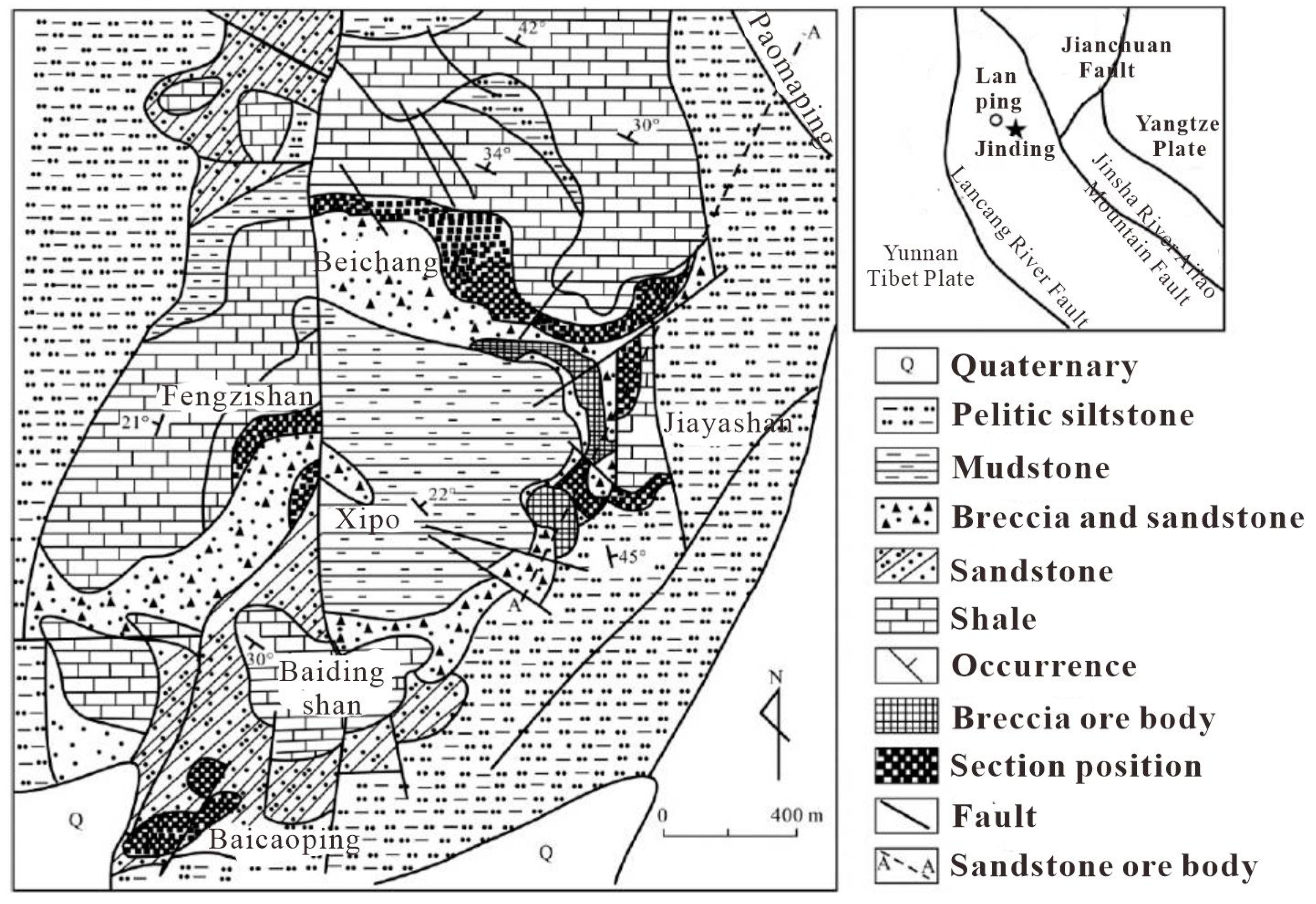
The Jinding Lead-Zinc Deposit is prominently situated within the densely compressed middle segment of the Sanjiang Fold System, positioned precisely at the northern terminus of the Lanping-Simao Meso-Cenozoic depression. It is strategically positioned between the north-south oriented faults tightly hemmed in by the Mishahe Fault Zone and the Lancang River Fault Zone, and is found to the western flank of the Bihe River Fault Zone, within the ancient Lanping-Yunlong Paleocene graben basin.The deposit is meticulously divided into seven distinct mining sections, including Beichang, Jiayashan, Fengzishan, Paomaping, Xipo, Nanchang, and Baicaoping. The mining area exposes a succession of strata ranging from the older to the younger, comprising the Upper Triassic Sanhedong Formation (T3s) of marine limestones (including brecciated limestones, dolomitic limestones, argillaceous limestones, and limestone mudstones), the Maichuqing Formation (T3m, the core strata of the syncline, with alternating layers of quartz sandstones and carbonaceous mudstones), the Middle Jurassic Huakaizuo Formation (J2h, interbedded layers of argillaceous siltstones, siltstones, and mudstones), the Upper Jurassic Bazhulu Formation (J2b, consisting of mudstones, argillaceous siltstones, and calcareous conglomerates), the Lower Cretaceous Jingxin Formation (K1j, with alternating layers of quartz sandstones, silty mudstones, and intercalated limestone conglomerates), the Upper Cretaceous Nanxin Formation (K2n, composed of argillaceous conglomerates, fine sandstones, siltstones, and mudstones), the Upper Cretaceous Hutousi Formation (K2h, characterized by long quartz sandstones), the Lower Tertiary Paleocene Yunlong Formation (E1y, interbedded layers of muddy gravelly rocks and argillaceous siltstones), the Guolang Formation (E2g, with alternating layers of argillaceous siltstones, silty mudstones, and intercalated fine sandstones), the Eocene Baoxiangsi Formation (Eb, featuring long quartz sandstones, conglomerates, sandstones, mudstones, and quartzites), the Upper Tertiary Pliocene Sanying Formation (N2s, with interbedded layers of conglomerates, sandy conglomerates, sandstones, and mudstones), and the Quaternary Pleistocene (Qp, sand and gravel layers) and Holocene (Qh, comprising gravels, sand grains, and sandy clays).
Figure 1.
Simplified Geological Map of the Jinding Mining Area, Yunnan Province.
Figure 1.
Simplified Geological Map of the Jinding Mining Area, Yunnan Province.
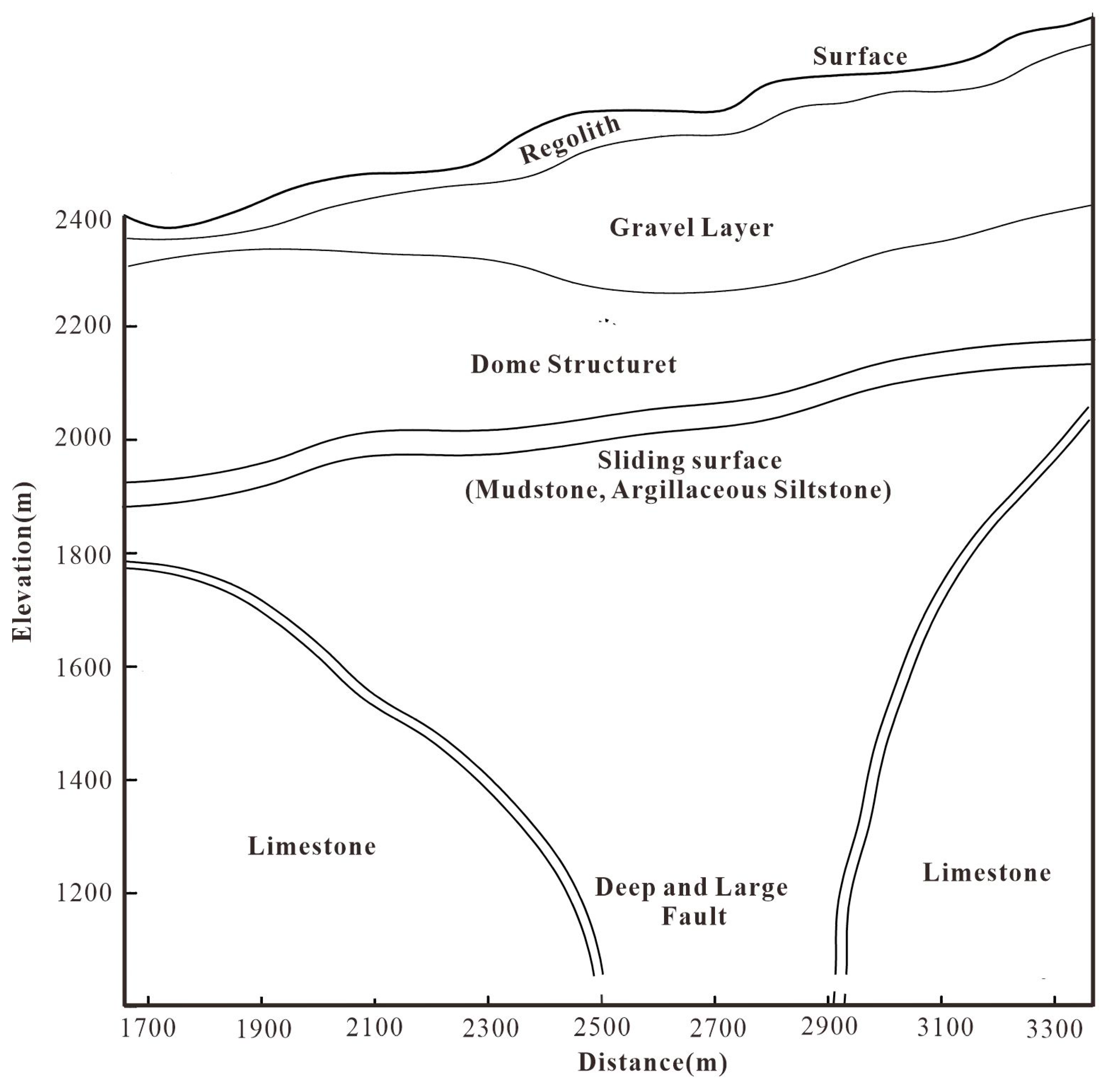
The primary geological structure of the mining area is a thrust nappe tectonic assemblage, which constitutes a significant component of the large-scale thrust nappe structure that formed during the Paleocene Yunlong period in the Lanping Basin. Klippe structures, or flysch formations, exist in numerous segments throughout the mining area. Furthermore, the thrust-sliding planes have also been incorporated into the tectonic domes, resulting in the formation of dome structures that are characterized by the co-deformation of both thrust tectonics and in-situ systems. In accordance with the preceding findings, it can indeed be concluded that the thrust tectonics predate the formation of the dome structures, with their inception likely commencing as early as the late Yunlong period. In summary, the geological structures of the Jinding mining area are complex, characterized by well-developed folds and faults that exhibit multiple stages of activity. This underscores the dynamic and protracted geological history of the region. The geological structures of the mining area are primarily characterized by the Gaoping-Laomujing syncline, the Bihe River Fault, horizontal thrust faults, transverse faults, oblique faults, and secondary fault structures.
2.2. Geological and Geophysical Model of the Ore Deposit
Based on the existing geological data, physical property measurement and 2D geological model[
15] (
Figure 2), we have constructed a 3D geophysical model of Jinding lead-zinc deposit, as shown in the
Figure 3.
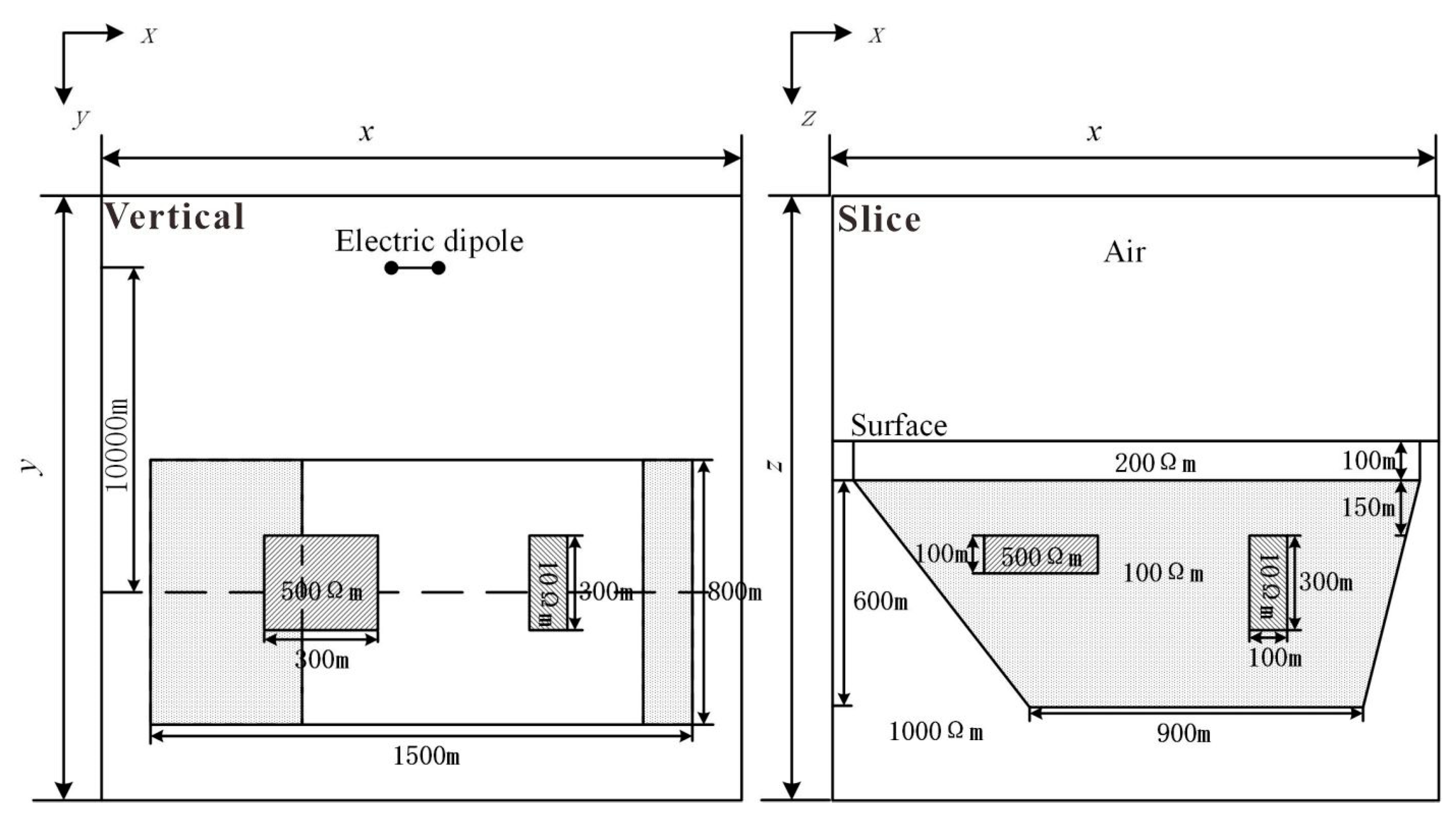
In the
Figure 3, the first layer represents the surface covering layer with a thickness of 100m. Its main component is sand and gravel strata, and it has an average resistivity of 200
. Beneath the covering layer lie domes and concealed deep fault structures with a resistivity of 100
. On both sides of the fault are high-resistance surrounding rocks with a resistivity of 1000
. The ore bodies are hosted within the dome structure, primarily consisting of sandstone-type and limestone breccia ore bodies. The sandstone ore body resembles a platy form, with a resistivity of 500
. Its dimensions are 300m in length, 100m in width, and 300m in height. The limestone breccia ore bodies often appear as inclined or vertical thin layers, also with a resistivity of 500
, and their dimensions are 100m in length, 300m in width, and 300m in height. The limestone breccia ore bodies often occur as inclined or vertical thin layers with a resistivity of 500
. Their dimensions are typically 100m in length, 300m in width, and 300m in height.
2.3. The Coupled Finite-infinite Element Method of CSAMT
Numerical simulation research not only enhances people's understanding and knowledge about the exploration methods, but also assists in selecting the correct exploration approach and setting appropriate field acquisition parameters. Therefore, we employed a three-dimensional CSAMT forward modeling program, based on the coupled finite-infinite element method to conduct a numerical simulation on the geophysical model of Jinding lead-zinc mine. The 3D CSAMT forward modeling using the finite-element and infinite-element coupling method is an efficient numerical simulation technique for electromagnetic fields, which combines the advantages of the finite element method in handling complex geological structures and boundary conditions with the characteristics of the infinite element method in simulating infinite far-field attenuation. This method achieves rapid and high-precision forward modeling, reduces the computation domain and the number of nodes, accelerates the computation, and is of great significance to the development of exploration geophysics[
20,
21].
2.3.1. Fundamental Equation
The electric field generated by a horizontal electric dipole ( time factor
, angular frequency
) in an isotropic conductive medium satisfies the double curl equation [
22]:
where
is the resistivity,
is the current density vector of the electric dipole, and the magnetic permeability
of both the air and the subsurface medium is taken as the vacuum magnetic permeability, while the dielectric constant
is the vacuum dielectric constant.
The electric dipole source exhibits singularity. The total electric field is decomposed into the sum of the background field
(primary field ) and the induced field
(secondary field ). The background field
is directly solved using a one-dimensional geoelectric model[
23], while the induced field
is solved using the finite element method to avoid the calculation of source singularity.
The background field
also satisfies the double curl equation of the electric field. Equations (1) and (2) can be used to derive the double curl equation based on the secondary field
:
where
. We know that on an electrical interface, the normal component of the electric field is discontinuous, while nodal finite elements require the electromagnetic field to be continuous in the normal direction. Therefore, the obtained finite element solution is often inaccurate and needs to be corrected. In the source region, the electric field solution of nodal finite elements does not satisfy condition
; in the source-free region, it does not satisfy condition
. A divergence correction condition needs to be added to Equation (3) [
24].
2.3.2. Weak Solution Integral Form
Based on the weighted residual finite element method (Jin 2014), establish the residual formula for Equation (4):
Take any test function
, on the region
:
Let S be the outer boundary surface of the region
. Instead of using traditional truncated boundary conditions, infinite elements are employed. Within the infinite elements, the electromagnetic field decays to zero, so we have:
By applying the first vector Green's theorem, Equation (6) can be simplified to:
Use finite element method to discretize the internal computation domain. Assuming there are n nodes in the internal computation domain, the j-th test function can be taken as:
2.3.3. The Coupled Finite-Infinite Element Method
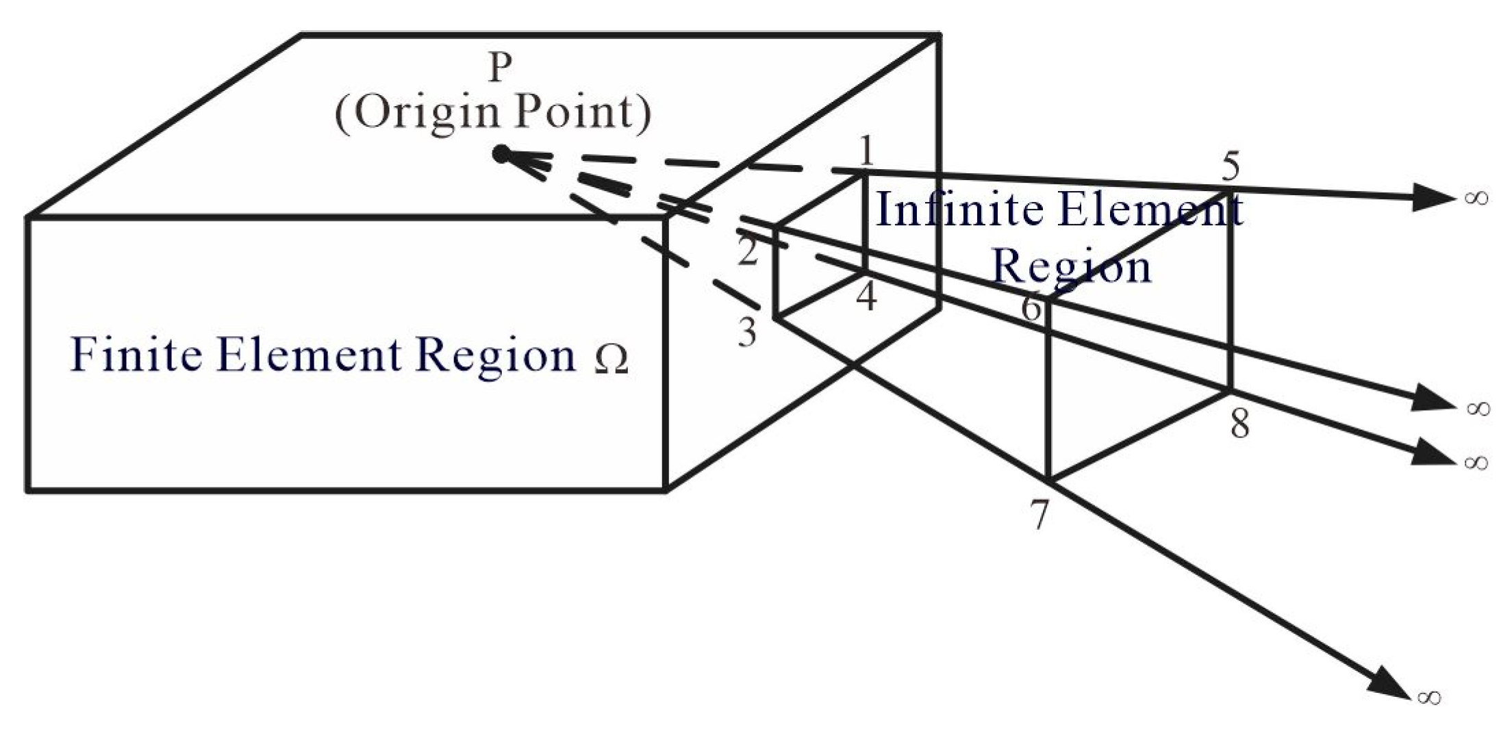
The coupled finite-infinite element method divides the entire solution domain into a finite element region and an infinite element region, replacing the traditional outer boundary with the infinite element region. Finite element analysis and infinite element analysis are performed in the two regions respectively, and they are combined through the assembly of the overall stiffness matrix for numerical solution.
Figure 4 is a schematic diagram of the division of finite element and infinite element calculation regions. In the figure, the finite element region is the target region, which includes the field source, target body, measurement points, etc.; the infinite element region extends from the boundary of the finite element region to infinity, serving as the boundary calculation region. Infinite element analysis involves using infinite element mapping and shape functions in a certain direction within this region to map the global coordinates to local coordinates. Its principle is the same as that of finite element analysis.
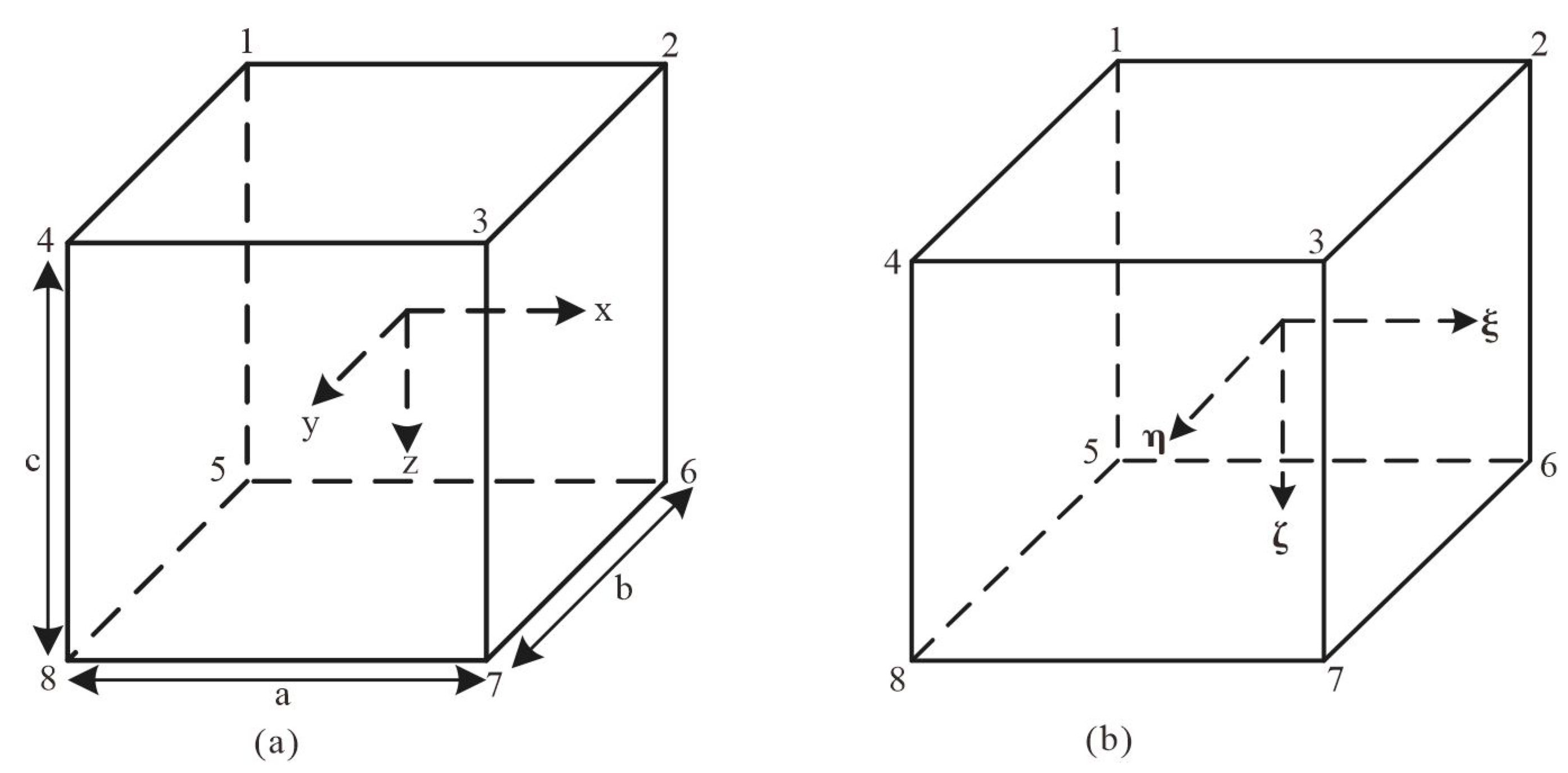
When performing finite element analysis, the rectangular hexahedron is used for regional discretization, and the element node numbering and coordinates are shown in
Figure 2.
In
Figure 5, the corresponding relationship between the coordinates of the parent and child elements is as follows:
Where
,
,
represent the midpoint of the child element, and a, b, c represent the three side lengths of the child element. The expression for the shape function of the rectangular hexahedron is as follows:
In the equation, , , represent the coordinates of node i in the child element within the parent element.
- 2.
The Infinite Element Analysis
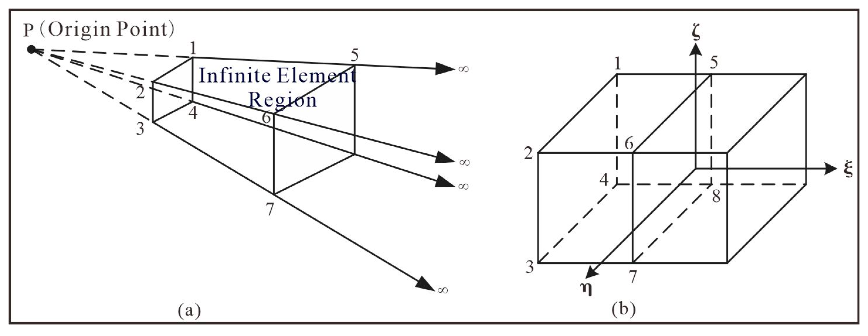
When performing infinite element analysis, a three-dimensional eight-node Astley-type infinite element is used[
25].
Figure 3 is a schematic diagram of three-dimensional infinite element mapping, where nodes 1, 2, 3, 4, 5, 6, 7, and 8 are the basic elements of the infinite element. P is the coordinate origin, and nodes 1, 2, 3, and 4 are the four nodes of a finite element on the boundary. The distances from point P to nodes 5, 6, 7, and 8 are twice the distances from point P to nodes 1, 2, 3, and 4, respectively. Infinite element analysis involves mapping infinite coordinates to local coordinates in
Figure 3(b) through infinite element mapping. In
Figure 3(b), the four outermost nodes of the infinite element represent infinity, and their field values are zero.
In
Figure 3(b),
represents the mapping direction of the infinite element. Within plane
, the infinite element and the finite element adopt the same mapping form and shape function. The coordinate mapping for the infinite element is as follows:
Li represents the area of the quadrilateral,
Combining the coordinate mapping relationship in direction
, the coordinate mapping function for the 8-node infinite element can be obtained:
Where:
quadrilateral surface element mapping and linear interpolation of area coordinates
For the shape function of the infinite element, its specific expression is as follows:
This shape function is the product of the coefficient A used in the shape function adopted in the Astley Mapped Infinite Element Theory (Astley, 1994) and a second-order Lagrange interpolation polynomial.
The finite element and infinite element analysis are basically consistent, both being eight-node elements. Therefore, in numerical simulations, the infinite elements and finite elements can be perfectly combined to ensure the symmetry of the stiffness matrix, making the solution simple and convenient.
2.3.4. Solving the Equation System
In the three-dimensional numerical simulation of CSAMT, each node has three degrees of freedom in the x, y, and z directions. Therefore, we take:
Where, is the shape function of the j-th measurement point, and its specific form is detailed in equations (11) and (14).
Equation (9) can be written as:
Using the vector curl formula and the divergence formula, Equation (16) above can be simplified and written in matrix form as follows:
where:
Equation (17) is a large, sparse, symmetric complex coefficient linear equation system. In this system, matrix A represents the overall stiffness matrix of the coupled finite element-infinite element method, which is an order square matrix. Here, , , enote the total number of nodes in the x, y, and z directions, respectively. Each row in matrix A has a maximum of 81 non-zero elements. x represents the electric field values at each node that need to be solved; b is the right-hand side term, which includes the anomalous body and the primary field. For solving large-scale sparse linear equation systems, this paper adopts Pardiso, an open-source solver with excellent performance and high parallelization. Pardiso uses LU decomposition for direct solving, making it particularly suitable for handling multi-source CSAMT problems.
2.4. The Forward Modeling of the Jinding Lead-Zinc Geophysical Model
We use the coupled finiment-infiniment element method, the forward modeling calculation parameters are as follows:
In the x direction, the subdivision area ranges from -3000 to 15000. Within the survey line area, the grid size is set to 50 meters, resulting in a total of 121 nodes.
In the y direction, the subdivision area ranges from -3000 to 3000. Within the survey line area, the grid size is set to 50 meters, resulting in a total of 63 nodes. Near the field source and the target body, the grid subdivision is relatively dense.
In the z direction, the subdivision area ranges from -3200 to 3000, with a total of 36 nodes. The air region spans from -3200 to 0, and is subdivided into 6 layers. Due to the rapid attenuation of the field in underground media, the grid subdivision size is smaller, the grid size is set to 25 meters.
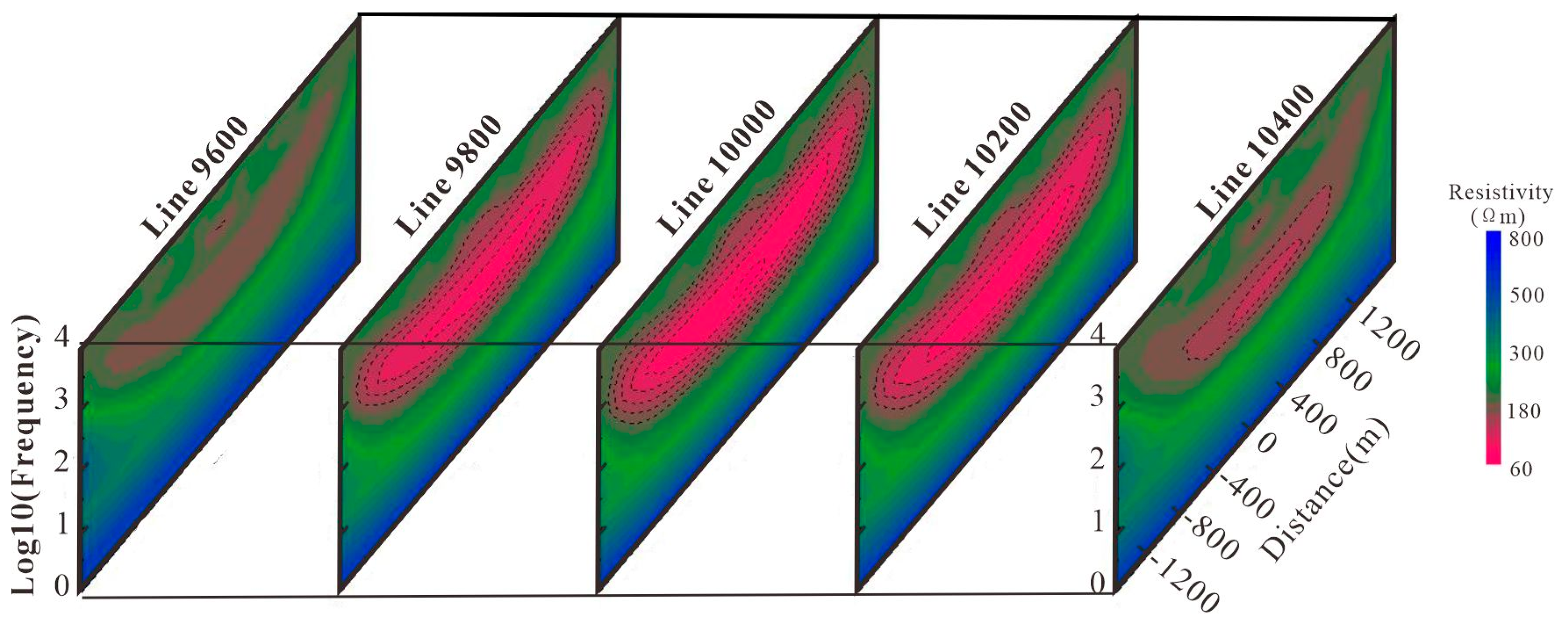
Frequencies: 8192, 4096, 2048, 1024, 512, 256, 128, 64, 32, 16, 8, 4, 2, 1 Hz, totaling 14 frequencies. The average calculation time for each frequency point is approximately 240 seconds. The numerical simulation results are presented in
Figure 4.
In
Figure 7, from left to right, the vertical source-receiver distances of the five survey lines are 9600m, 9800m, 10000m, 10200m, and 10400m, respectively. From the apparent resistivity pseudo-section map , it can be observed that the CSAMT 3D forward modeling results exhibit a significant response to the low-resistivity dome structure of the Jinding lead-zinc deposit, and provides a clear reflection to the structure's morphology. However, due to the boundary effects, the boundary between the dome structure and the high-resistivity limestone is relatively blurred. In addition, due to the low-resistivity shielding effect of electromagnetic methods, the relatively high-resistivity lead-zinc ore bodies show little response in the simulation. Based on the numerical simulation results, it can be seen that when exploring for high-resistivity target bodies in low-resistivity surrounding rocks, the CSAMT electromagnetic response is weak, and the numerical effect is not significant. However, when exploring for low-resistivity structures such as faults and fracture zones in high-resistivity surrounding rocks, the effect is very pronounced. Therefore, it is feasible to conduct CSAMT exploration research in the Jinding lead-zinc mining area to identify low-resistivity faults, dome structures, and other features within the ore deposit.
Additionally, the forward modeling parameters used in the 3D CSAMT numerical simulation, such as grid size, vertical source-receiver distance, frequency band range, survey line length, as well as the three-dimensional size and location of the target body, can assist us in designing the field CSAMT acquisition parameters to achieve good exploration results.
3. Acquisition Design for CSAMT
The objective of the CSAMT exploration is to obtain the electrical structure within a depth of 1km below the surface of the mining area, and help us to understand the deep geological background and mineralization environment, at the same time, it can provide geophysical evidence for geological researchers to study the genesis of the Jinding lead-zinc deposit, and if it is possible, which can predict and delineate the mineralization target areas.
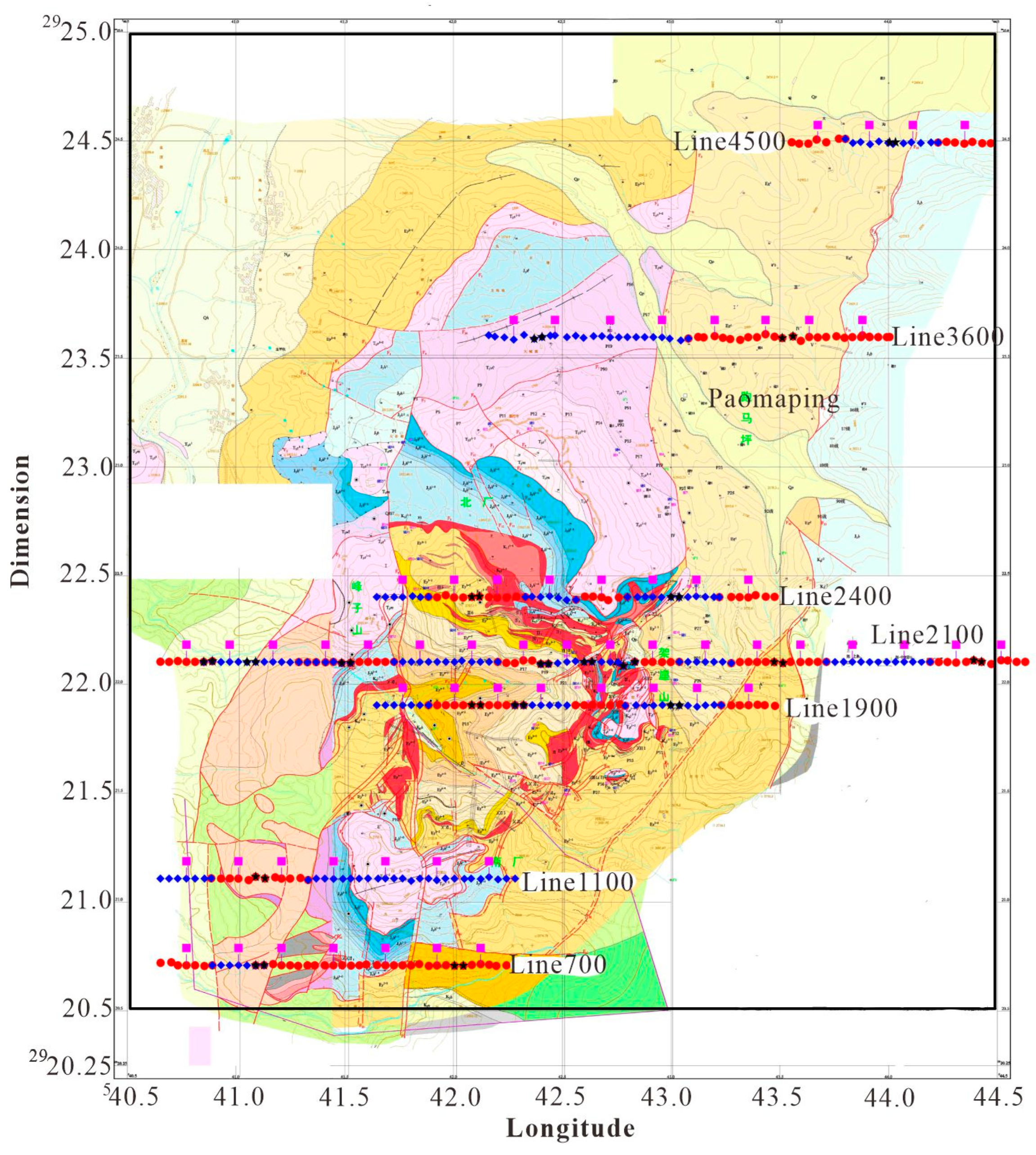
3.1. Line Layout
For the CSAMT field data acquisition, a total of 7 survey lines were laid out. The specific locations of the survey lines are shown in
Figure 5. From bottom to top in the figure, they are Line 700, Line 1100, Line 1900, Line 2100, Line 2400, Line 3600, and Line 4500. The total length of the survey lines is 13.68 kilometers. Among them, Lines 1900, 2100, and 2400 cross the main ore body and are the key research objects.
3.2. Acquisition Parameter
The parameters for CSAMT field data acquisition mainly consist of two parts: transmitter parameters and receiver parameters. The transmitter operating parameters primarily include the transmitter position (transmitter-receiver distance), dipole length : AB, ground resistance: RAB, transmitting current : I, and transmitting frequency: f. The receiver operating parameters mainly include the measurement mode, receiver MN length, and acquisition time.
For this CSAMT field measurement, the transmitter dipole AB= 2.25km, ground resistance RAB,=20
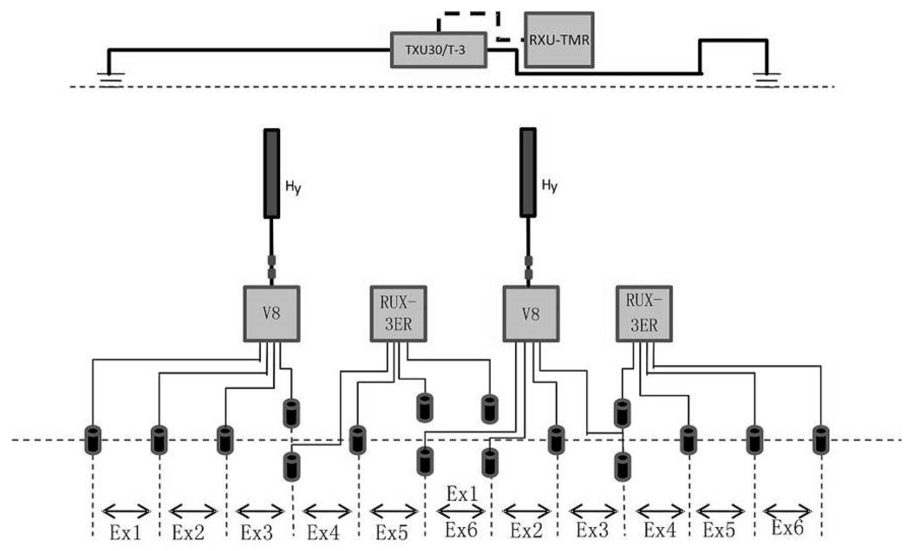
. To ensure an exploration depth exceeding 1km, based on the previous forward modeling parameters, the transmitter-receiver distance is set between 10.8km and 14.2km. The transmitting frequency ranges from 7680Hz to 0.9375Hz, with a total of 52 frequency points. The dipole spacing MN =40 m. The CSAET method is adopted for the field CSAMT measurement, with 6 channels of electric field data and 1 channel of magnetic field data collected each time. Two sets of V8 multifunctional electrical instruments are used for field data acquisition. The construction layout is shown in
Figure 9.
3.3. Quality Control and Analysis for the CSAMT Data
In the field data acquisition, the strength of the received signal and the duration of data collection are crucial to the quality of CSAMT data acquisition. Therefore, in this CSAMT field measurement, on the one hand, through white noise measurement experiments, the signal-to-noise ratio was calculated to judge the strength of the received signal, and the transmission signal strength was adjusted accordingly. On the other hand, through data collection time experiments, the quality of measurement data under different collection times was analyzed to find the optimal data collection time scheme.
3.3.1. CSAMT Signal-to-Noise Ratio Experiment
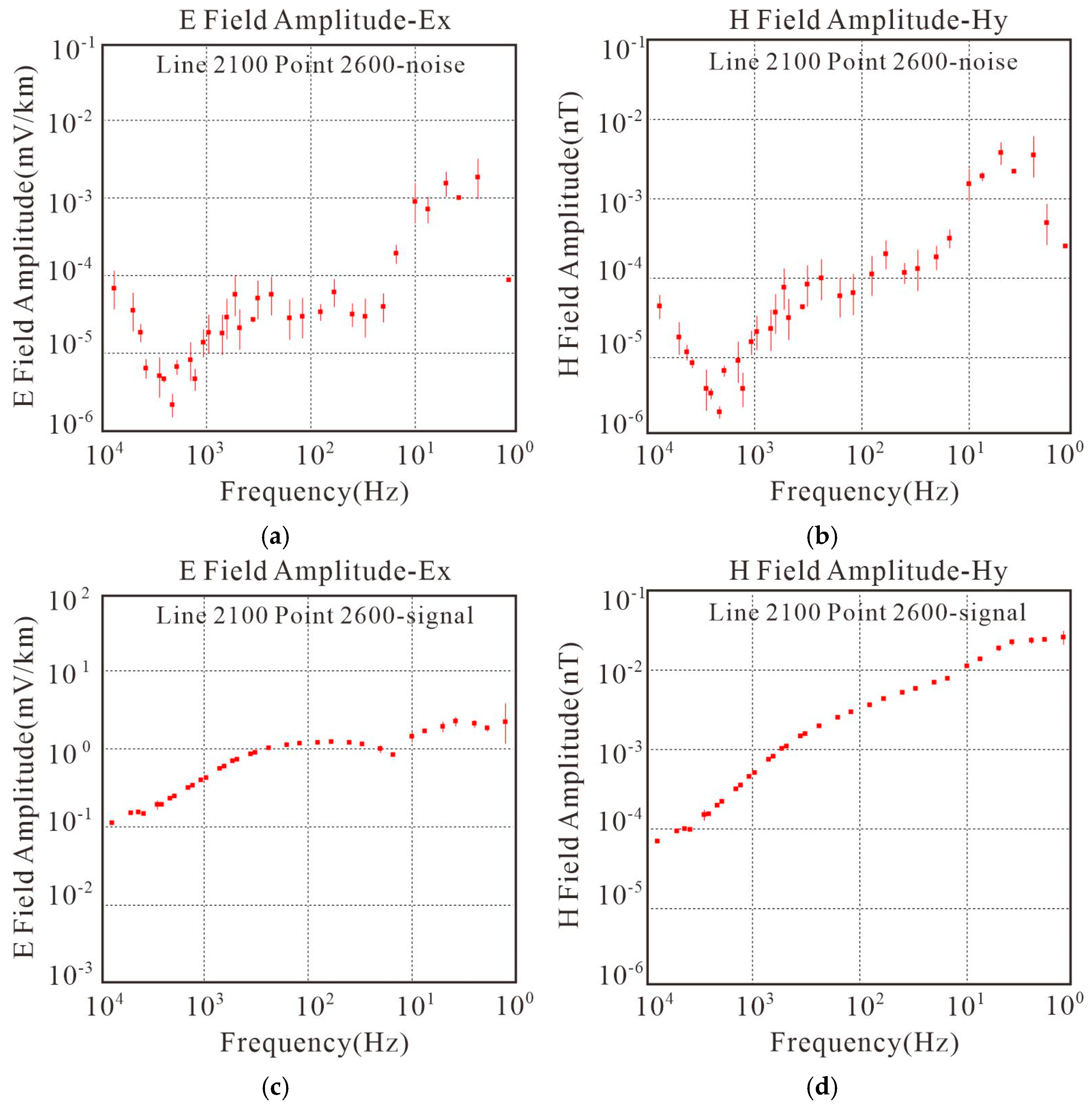
To calculate the signal-to-noise ratio (SNR) of CSAMT data, both the noise signal and the data signal need to be obtained. Firstly, the open-pit mine at the center of the work area was selected as the experimental site. Data acquisition was conducted when the artificial field source was not transmitting, and the measured signals were considered as noise signals. Secondly, under the same experimental setup conditions, when the artificial field source was transmitting, the collected signals were considered as data signals. Finally, the signal-to-noise ratio (SNR) formula was used to calculate the SNR. By comparing the SNR values, the quality of the collected data was evaluated, which further indicated the strength of the received signal. The experimental results of the signal-to-noise ratio were shown in
Figure 10.
In
Figure 10, there are four sub-figures: the electric field noise signal amplitude diagram, the magnetic field noise signal amplitude diagram, the electric field data signal amplitude diagram, and the magnetic field data signal amplitude diagram. From the experimental results, it can be observed that the noise signals have a large range of amplitude value fluctuations and significant error bars. On the other hand, the data signals exhibit smooth and continuous amplitude curves with small error bars, and their values are more than 10 times those of the noise signals. Therefore, the signal-to-noise ratio experiment we designed is reasonable and feasible, and can be used as a criterion for evaluating the strength of the received signal.
The calculation formula for signal-to-noise ratio is as follows:
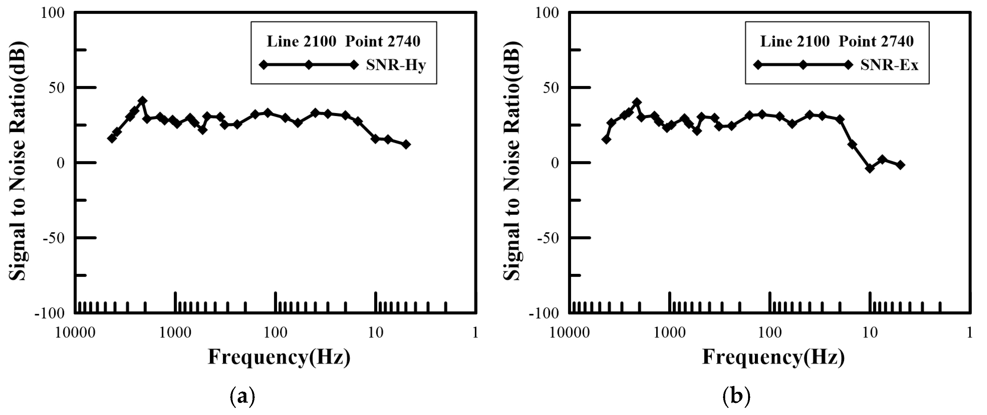
The calculation results of the signal-to-noise ratio for the electric field and magnetic field at the test point are shown in
Figure 11.
In the
Figure 11, within the frequency band of 5000-10 Hz, the signal-to-noise ratio of both the electric field and the magnetic field is greater than 20 Db, and the noise percentage is less than 10%. This indicates that the signal strength is sufficiently large, and the quality of the measured CSAMT field data is high. In the high-frequency and low-frequency bands, the SNR is less than 10 Db, and the noise percentage is greater than 30%, indicating low quality of the collected data. This is due to two main reasons: on the one hand, the V8 instrument and magnetic probe exhibit response distortion in both high and low frequency bands, resulting in low measurement accuracy; on the other hand, when transmitting high frequencies, the transmission current is small, making the signal more susceptible to interference. In the case of low frequencies, factors such as shorter data collection time and stronger interfering signals contribute to a relatively lower signal-to-noise ratio in the data.
3.3.2. The Experiment of CSAMT Data Acquisition Time
During the field work, we also conducted experiments on acquisition time, and obtained apparent resistivity sounding curves for different acquisition times. Through comparative analysis, we determined the optimal acquisition time parameters.
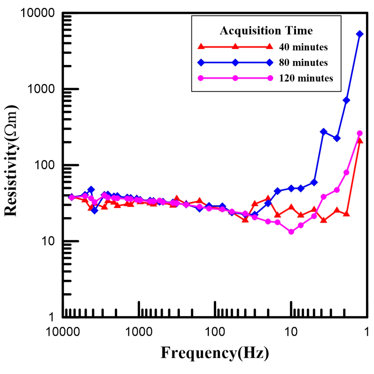
Experimental conditions: With a single acquisition cycle of 40 minutes, three acquisition times of 40, 80, and 120 minutes were selected. Under the same survey line, survey point, equipment, and field source, three apparent resistivity sounding curves were obtained. The experimental results for different acquisition times are shown in
Figure 9.
As can be observed in
Figure 12, the apparent resistivity sounding curve with an acquisition time of 40 minutes exhibits poor continuity of resistivity values, especially below 30 Hz. The apparent resistivity curve appears jagged, and the characteristics of the transition zone and near zone are not pronounced, indicating poor data quality. Compared to the apparent resistivity curve of 40-minute, the apparent resistivity sounding curve with an 80-minute is smoother and more continuous, with smaller jumps. Below 30 Hz, it starts to enter the near zone, and the curve rises at an angle exceeding 45°. Meanwhile, there are jump points, and the transition zone characteristics are not pronounced, indicating intermediate data quality.The apparent resistivity sounding curve with 120-minute acquisition time is smooth and exhibits good continuity. The characteristics of the far zone, transition zone, and near zone are distinct. A minimum value appears at 10 Hz, which is a characteristic of the transition zone. Below 10 Hz, the sounding curve rises at nearly a 45-degree angle, which is a typical characteristic of a CSAMT sounding curve, indicating high data quality.
Therefore, in the Jinding lead-zinc mining area, by extending the data acquisition time and increasing the number of stacking, the characteristics of the apparent resistivity sounding curve at the measurement points can be significantly improved, thereby enhancing the quality of CSAMT single-point data.
4. CSAMT Data Processing and Inversion
4.1. CSAMT Data Processing
Before inversion, CSAMT data processing mainly includes the elimination of flying points and smoothing of the Cagniard apparent resistivity and phase data at each measurement point, as well as static correction and spatial filtering of apparent resistivity and phase along the entire survey line.
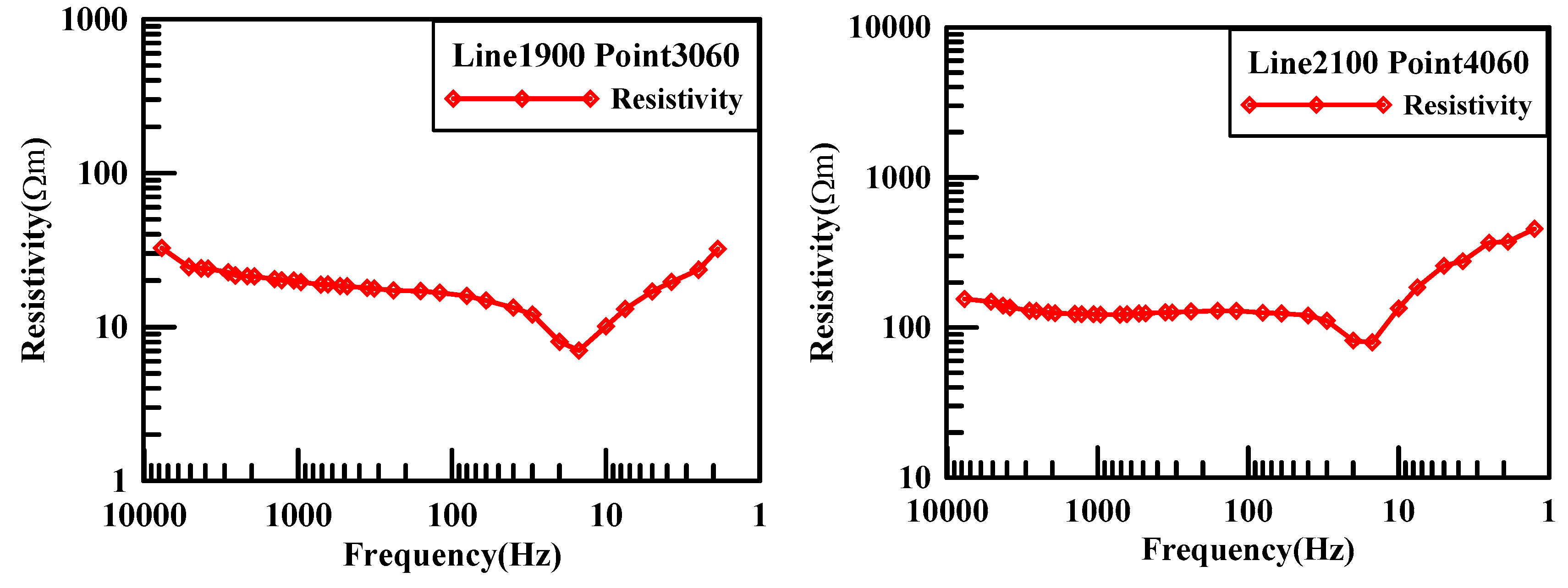
Figure 13 shows the apparent resistivity frequency sounding curve obtained after data processing for some measurement points. From
Figure 10, it can be seen that the apparent resistivity curve is smooth, continuous, and has a clear morphology. The characteristics of the far zone, transition zone, and near zone of the curve are obvious, which conform to the standards of CSAMT apparent resistivity sounding curves.
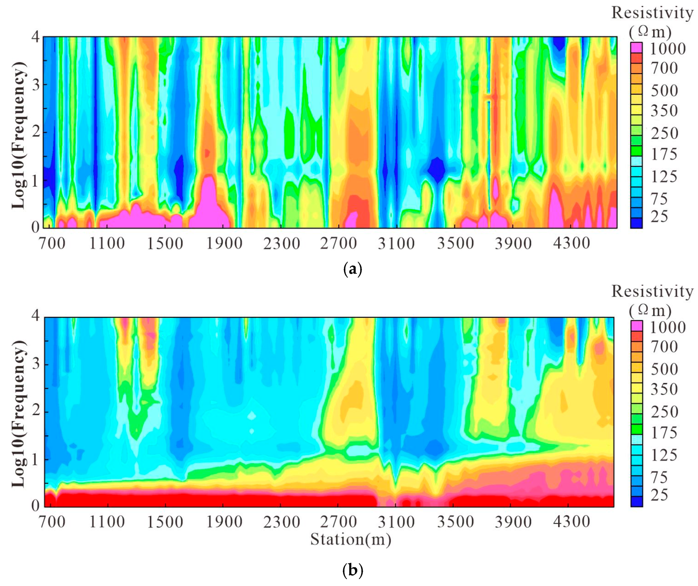
Figure 14 (a) shows the original pseudo-section of frequency-apparent resistivity for survey line 2100. It can be seen from the figure that due to the influence of uneven geological bodies and topographic fluctuations on the surface, the Cagniard apparent resistivity varies greatly and exhibits “noodle-like” characteristics in the vertical direction, indicating severe static effects that require processing.
Figure 14 (b) is the result diagram of the frequency apparent resistivity pseudo-section after static correction and spatial filtering. It can be seen from the figure that after processing, the apparent resistivity data changes smoothly, the vertical “noodle-like” phenomenon disappears, and the static effects are well suppressed.
From the sounding curves of apparent resistivity at the measurement points and the pseudo-section diagram of frequency-apparent resistivity along the survey line, it can be seen that compared with the original data, the processed data has achieved significant suppression in terms of static effects. The data is authentic, reliable, and of high quality, making it suitable for further inversion.
4.2. CSAMT Inversion
Because the direction of the survey lines is perpendicular to the trend of the ore body, we can use two-dimensional continuous medium inversion software to invert CSAMT data. The principle of continuous medium inversion is based on the assumption of continuous variation of electrical properties in the subsurface. It discretizes the subsurface space using numerical methods and adjusts the resistivity values of each unit to achieve the best fit between the forward electromagnetic field data and the observed data. The method is closer to the real subsurface conditions and is suitable for exploration in complex geological settings, providing higher precision information on the subsurface electrical structure[
26,
27].
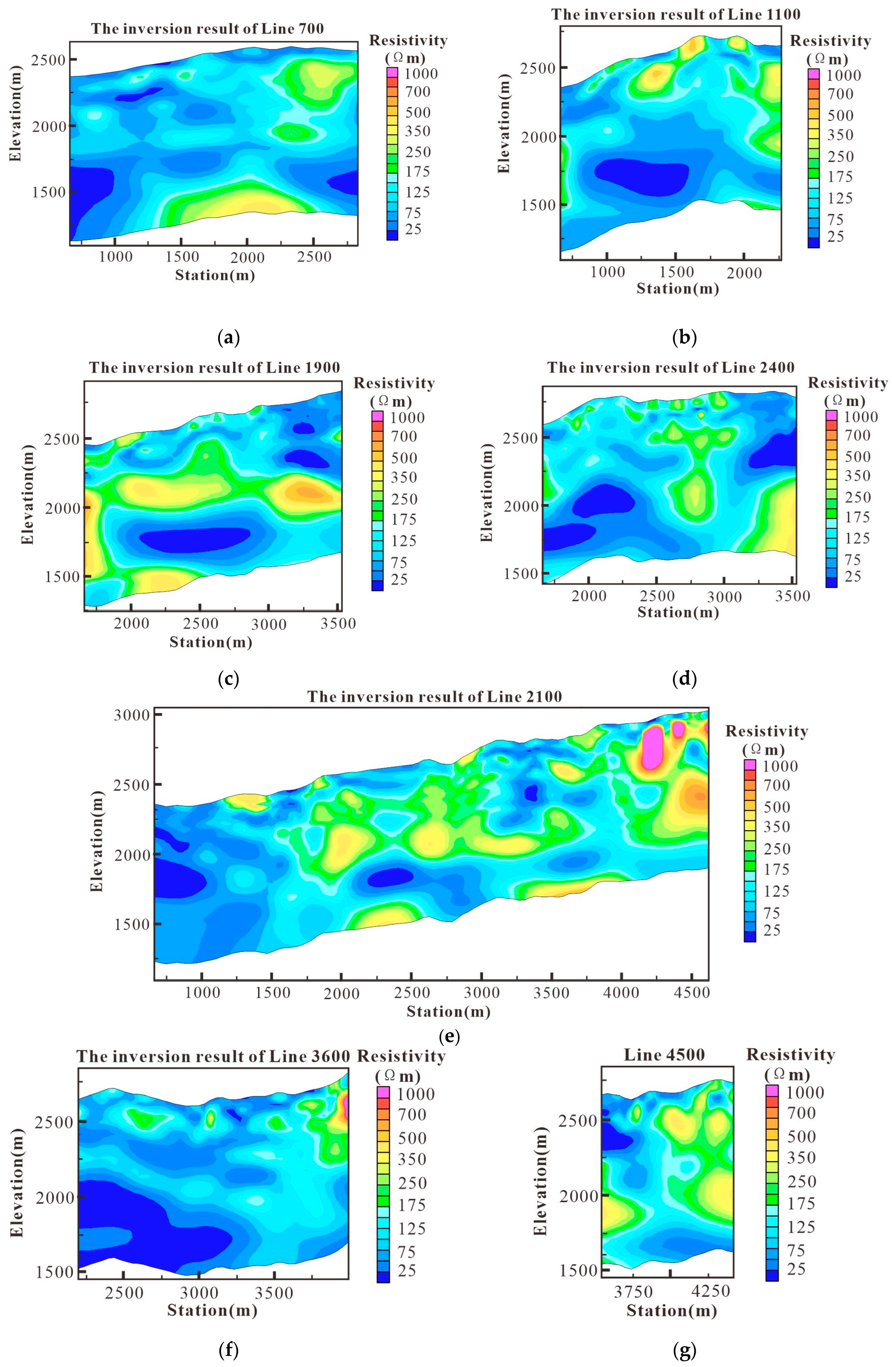
Based on the statistics of the work area, the frequency of measurement points entering the near zone is around 10Hz, and the surface resistivity ranges between 100-200 ohm-meters. According to the skin depth formula calculation, the exploration depth is approximately 1.5Km, which meets the exploration requirements. Therefore, we selected a total of 40 frequency points in the 8192-10Hz frequency band for inversion. The initial inversion model is the result of one-dimensional Bostick inversion. After 34 iterations of inversion, the data misfit is 2.7. The inversion results of each survey line are detailed in
Figure 15.
5. The Electrical Structure Interpretation of the Jinding Lead-Zinc Mine
5.1. Physical Property Analysis
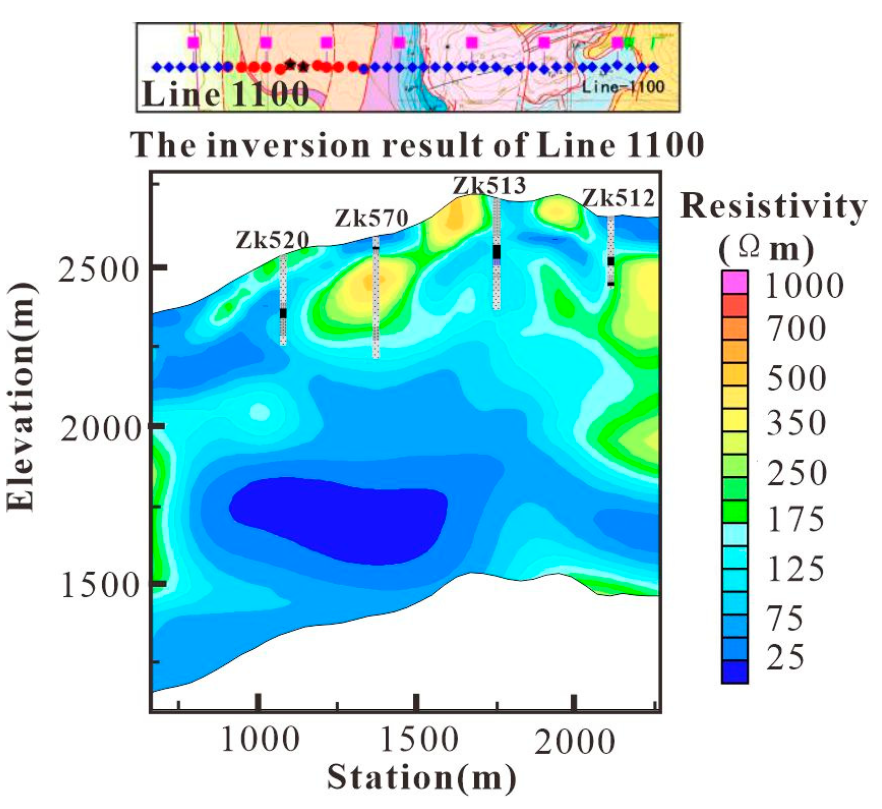
To interpret the electrical structure detected by CSAMT, this study used the two-dimensional inversion results of Line-1100 as a reference section. The main reason for selecting Line-1100 is that it has abundant borehole data, covering most of the stratigraphic lithologic units (including ore bodies) and major structural interfaces (including thrust nappes) in the mining area. The interpretation method we adopted is to combine the shallow subsurface electrical structure with borehole data, and then conduct a comparative analysis with the inversion results.
As shown in
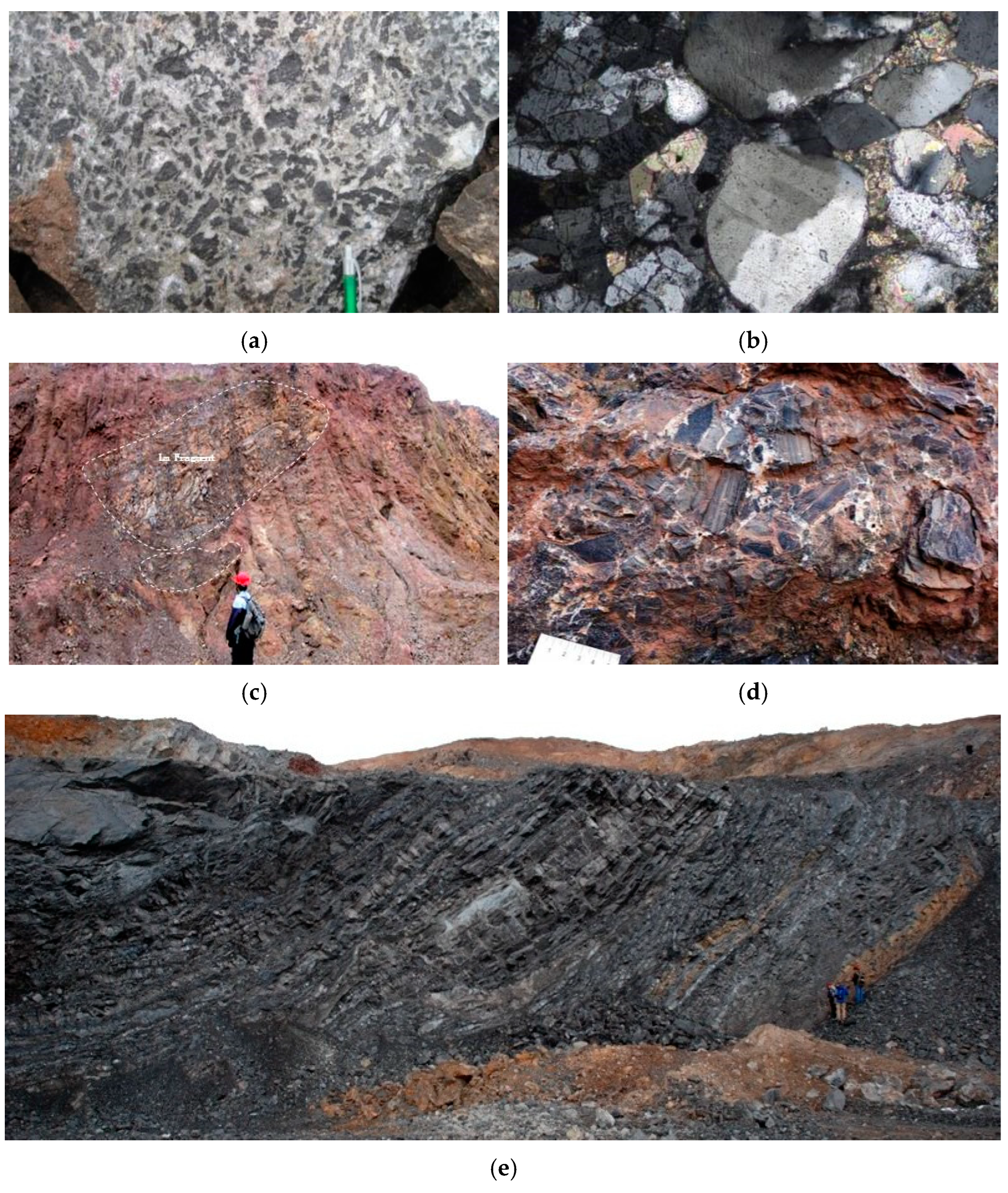
Figure 16, the profile exhibits a low-resistivity background. The central low-resistivity body primarily consists of fine sandstone, siltstone, limestone breccia containing lead-zinc ore and gypsum, with localized fault breccia zones.The center of the high-resistivity body is entirely composed of continuous fine sandstone and siltstone strata containing gypsum. Limestone, limestone breccia siltstone, as well as mudstone, sandstone, and siltstone containing gypsum exhibit moderate or high resistivity. From the above electrical patterns, it can be observed that the resistivity of geological bodies is controlled by the material composition and transport properties of the rocks themselves, with a more pronounced influence from the transport properties. Therefore, for the geological bodies in the Jinding mining area, due to the influence of large-scale tectonic and fluid activities, the distribution of their electrical conductivity is a response to the tectonic state and fluid type of the geological bodies.For example, rocks cemented by gypsum with low permeability exhibit high resistivity(
Figure 17a-b ), while breccia cemented by calcium or sand with high permeability exhibit low resistivity(
Figure 17c-d ). Relatively intact limestone and sandstone have moderate to high resistivity and occur as either independent stratigraphic systems or tectonically entrained rock slices (
Figure 17e). Therefore, the electrical structures of the subsequent survey line profiles are interpreted based on the electrical characteristics of the aforementioned geological bodies.
5.2. Interpretation of the Electrical Structure
The relative positions of the survey lines on the plane are shown in
Figure 4. Line-4500 and Line-3600 are located on the north side of the PaoMaping mining area; Line-2400, Line-2100, and Line-1900 pass through the Jiayashan mining area; Line 1100 and Line-700 are located on the west side of the Nanchang mining area. The north-south span of the survey lines is approximately 3.8km, and all survey line profiles are oriented east-west, which provides assistance for comparing the three-dimensional spatial positions of the underground electrical structures. Due to the significant differences and distinct contrasts in resistivity presented in the two-dimensional continuous medium inversion results, as well as the abundant details in the electrical structures, the interpretation of the electrical structures primarily relies on the two-dimensional inversion results.
- 3.
Line-2400
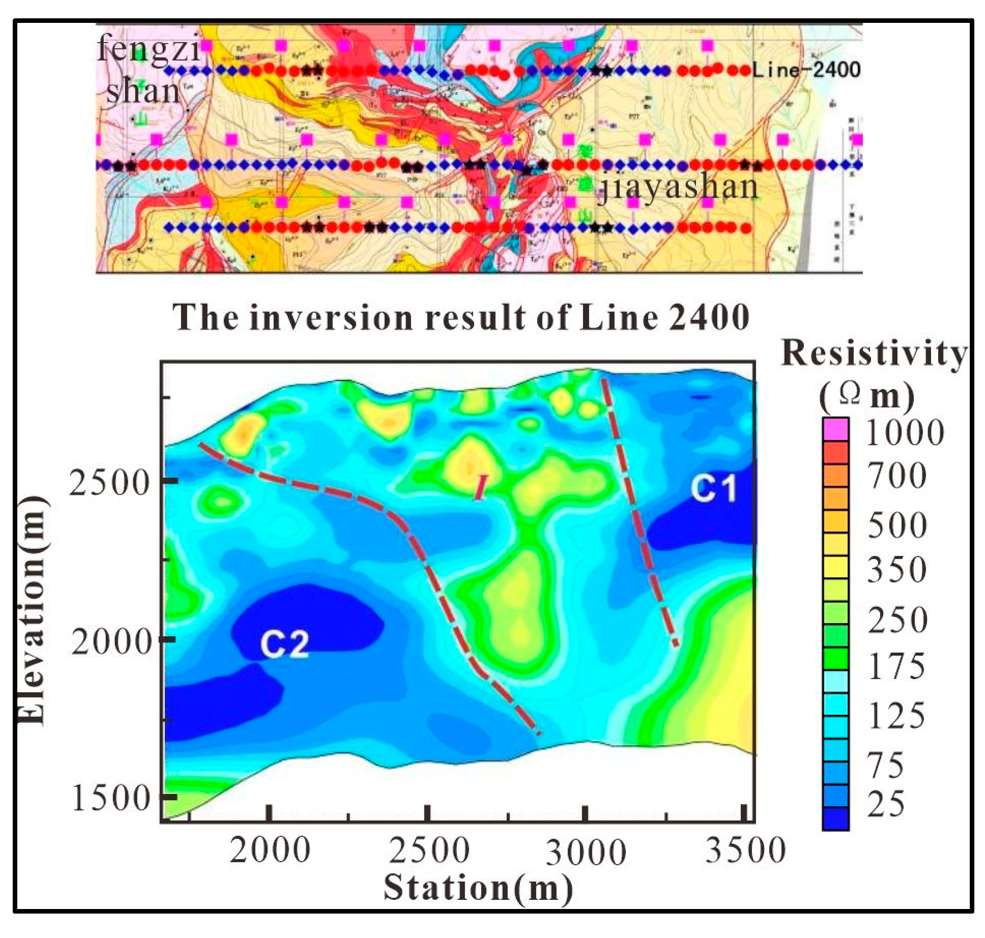
Line-2400, Line-2100, and Line-1900 are located in the Jiayashan mining segment of the Jinding mining area. As shown in
Figure 18, the entire profile of Line-2400 can be divided into three parts, with the western and eastern segments being high-conductivity areas, and the middle segment (Region I) being a high-resistivity area.Region I is the mineral occurrence segment, which exhibits alternating high and low resistivity from shallow to deep, reflecting a complex structural-rock system. The eastern segment is located below the outcropping area of the Guolang Formation (E2g), which is mainly composed of alternating layers of argillaceous siltstone and siltstone-bearing mudstone, with a high conductor C1 underlying it. The strata exposed in the western segment belong to the Yunlong Formation (E2y), with normal lithology consisting of alternating layers of muddy conglomerate and argillaceous siltstone, and there is a high conductor C2 present in the deep part. Based on the electrical characteristics of the rocks, the presence of high conductors C1 and C2 indicates that both sets of strata have undergone varying degrees of disruption and modification, resulting in increased conductivity compared to intact lithologies. From the electrical gradient zones, it can be observed that exogenous rock slices have been thrusted from west to east, overlying the Yunlong Formation strata. The mineral bodies are controlled by the thrusted base, while the Guolang Formation contacts the exogenous rock slices through high-angle strike-slip faults.
- 4.
line-2100
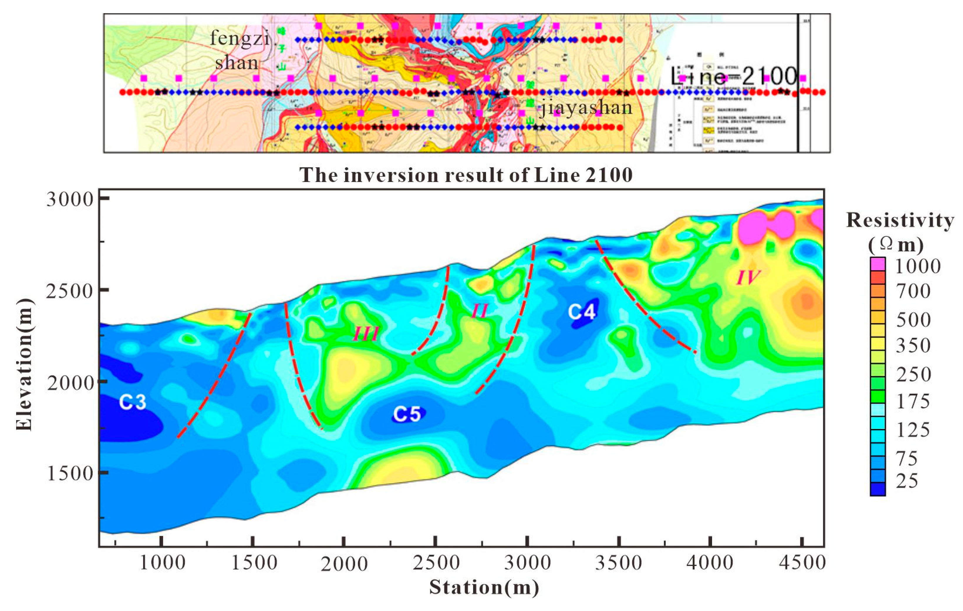
Line-2100 is the longest survey line, located to the south of Line-2400. As shown in
Figure 19, the electrical structure of the Line-2100 survey line is complex, being separated by five faults. Similar to Line-2400, Region II exhibits a high-resistivity background with alternating high and low resistivity from shallow to deep. However, the exposed area of the Yunlong Formation in Region IV on the west side is different from the western segment of Line-2400, showing high resistivity, which reflects a relatively intact J-K stratigraphic system. The difference between Region III and Line-2400 is that, although both are exposed areas of the Yunlong Formation, their electrical characteristics are completely opposite. The high-resistivity background indicates that the deep part of this region may have structural features similar to Region II. However, the presence of high conductor C5 corresponds to C2 in Line-2400. Similarly, high conductor C4 corresponds to C1 in Line-2400, reflecting the Guolang Formation. Additionally, there is a high conductor C3 on the west side of the Fengzishan mineral segment, which requires further investigation.
- 5.
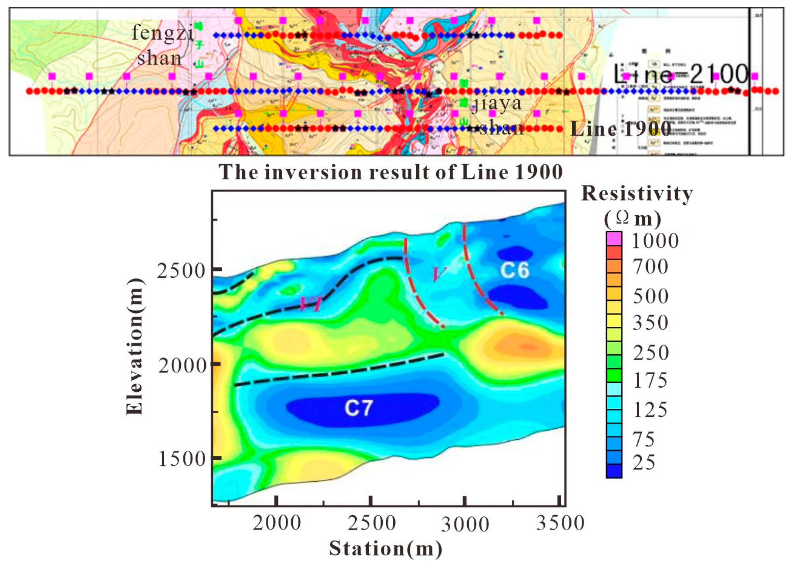
line-1900
Line-1900 is located to the south of Line-2100 and also crosses the Jiayashan mineral segment. The Line-1900 profile is divided into three parts by faults. The low-resistivity zone C6 in the eastern segment, compared with C1 in Line-2400 and C4 in Line-2100, indicates the stable electrical characteristics of the Guolang Formation in the north-south direction. However, the presence of the Bijiang Fault enhances the extent of the high conductor C6. The moderate resistivity in the middle mineral segment (Region V) shows slight differences from the electrical structures of the previous two survey lines. The western segment (Region VI) can be compared with Region III of Line-2100, with the difference being that Region VI has a wider distribution, and the underlying high conductor C7 can be connected to C5 in Line-2100.
- 6.
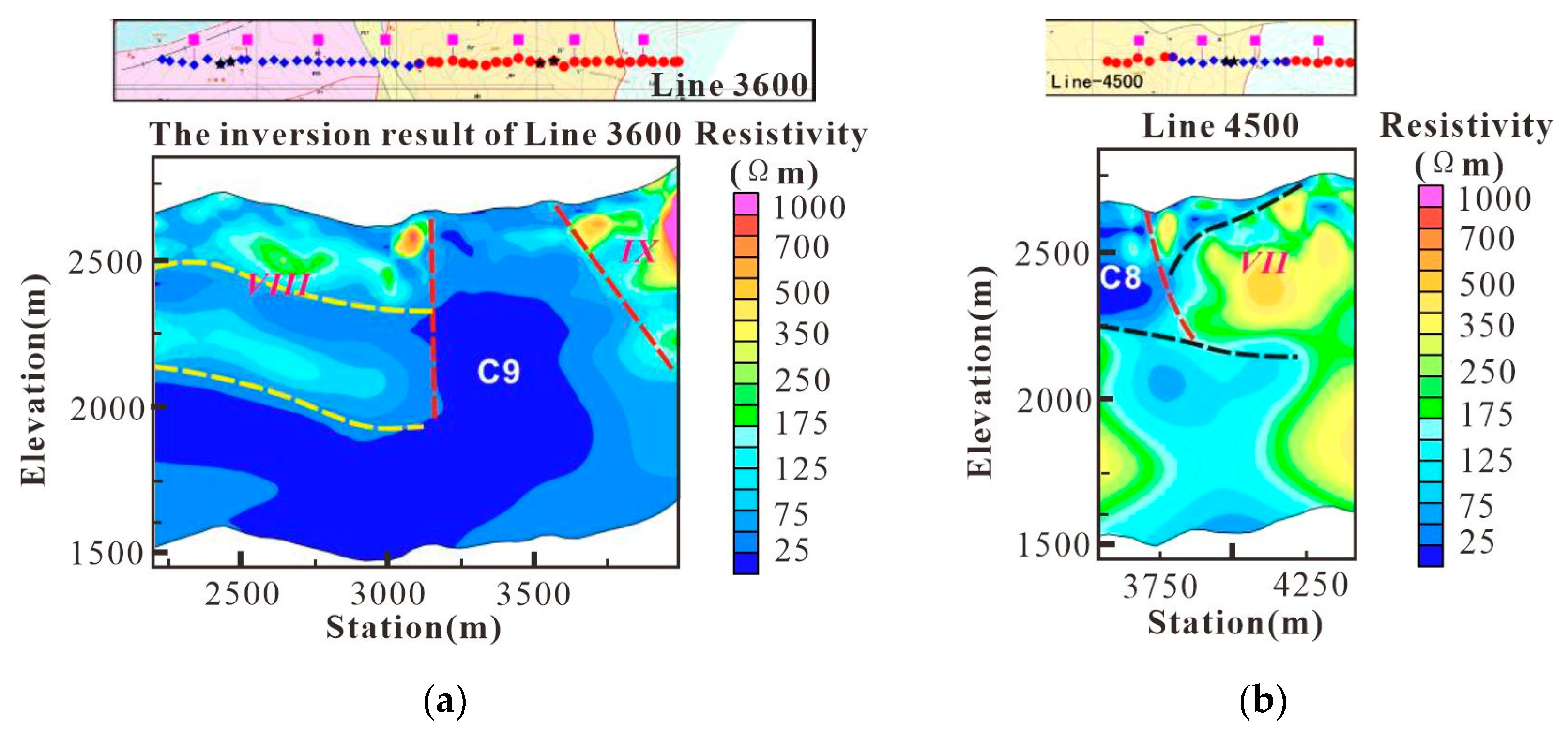
Line-4500 and Line-3600
Line-4500 and Line-3600 are located to the north of the Paomaping mineral segment, as shown in
Figure 21. In the electrical profile of Line-4500, Region VII reflects the J-K stratigraphic system. Similar to the previously mentioned survey lines, the Guolang Formation exhibits low resistivity (C8) and extends deeply downward. Line-3600 crosses three stratigraphic zones from west to east, which are T3, E2, and J2. The lateral electrical gradient zones also separate the fault occurrences in the three exposed stratigraphic zones. The high conductor C9 represents an extension of the Guolang Formation, and is connected to the deep part of Region VIII. The upper part may reflect an exotic thrust sheet, while the lower part belongs to the in-situ system. The vertical electrical gradient zone in Region VIII indicates the depth of the thrust surface.
- 7.
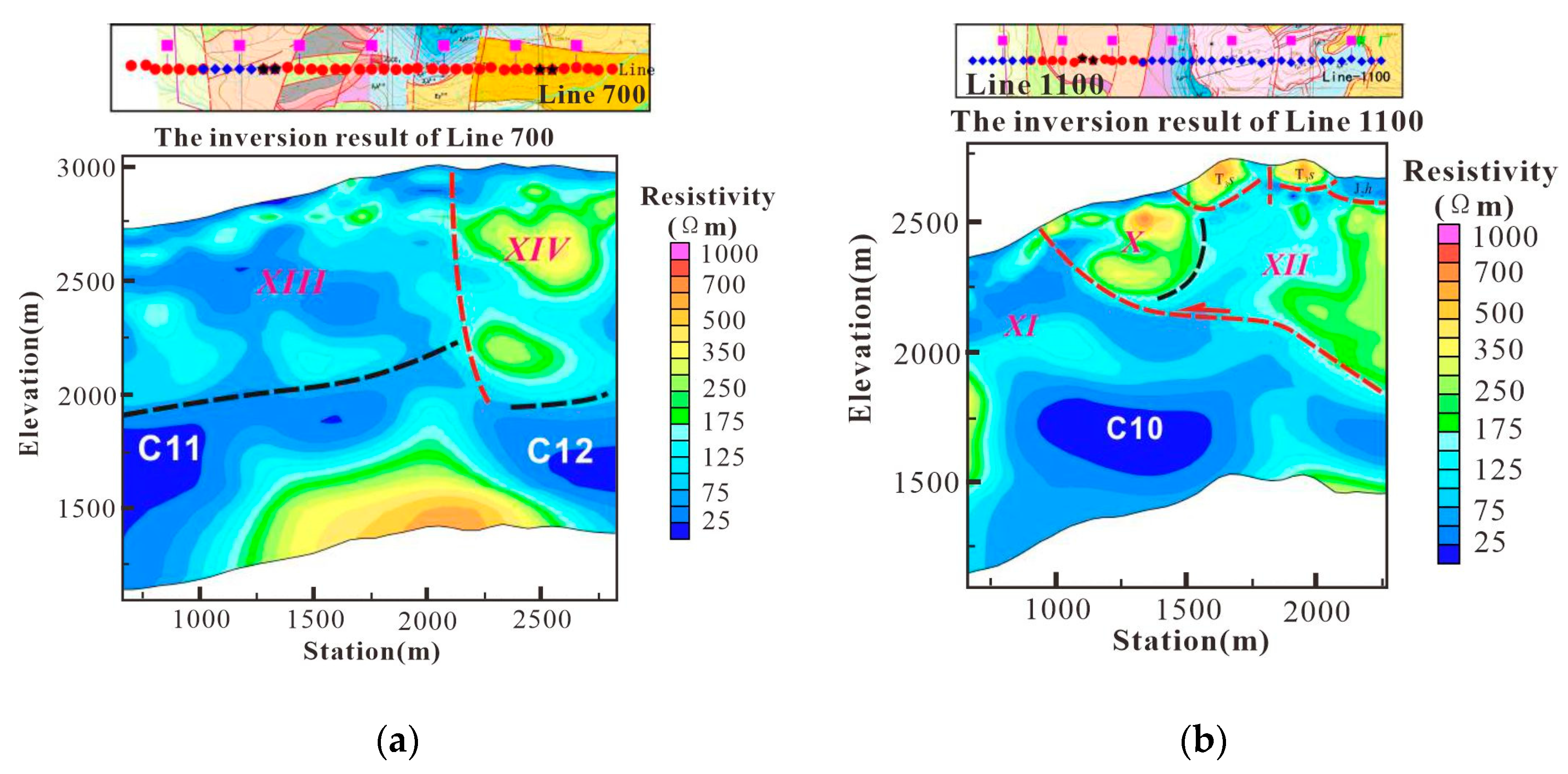
Line-1100 and line-700
Line-1100 and Line-700 are located to the south of the Jinding mining area and to the west of the Nanchang mineral segment. As shown in
Figure 22, the shallow high-resistivity bodies in Line-1100 outline the distribution of the exotic thrust bodies, while the in-situ stratigraphic system may be located in Regions XI and XII. Line-700 is situated to the south of Line-1100 and can be divided into eastern and western segments. The low-resistivity background in Region XIII indicates that the exotic thrust system is relatively thin, with the in-situ system dominating at depth. In Region XIV, the surface exposes strata of the Yunlong Formation, and the alternating high and low resistivity features may indicate that the stratigraphic system has undergone a certain degree of structural deformation or experienced large-scale fluid activity. Its electrical characteristics are similar to the mineralization system observed in the previously mentioned profiles.
Based on the interpretation of the electrical structure from the seven surveyed lines, it can be understood that the lithological system of the Jinding lead-zinc mining area is mainly divided into three parts: the exotic stratigraphic system, the middle lithological system, and the in-situ system. The electrical characteristics of the three lithological systems are as follows: the shallow exotic stratigraphic system is mainly characterized by a high resistivity background; the middle lithological system, influenced by tectonic and fluid cementation, displays alternating high and low resistivity; and the in-situ system is relatively complex, with the Yunlong Formation and Guolang Formation exhibiting different electrical characteristics. The Yunlong Formation shows significant electrical variations, while the Guolang Formation maintains low resistivity and high conductivity, and high conductors(C1, C4, C6, C8, C9) are prevalent in the underlying geological bodies of the exposed areas of the Guolang Formation.
6. Conclusion
We have developed a new exploration mode on the CSAMT. Based on the geological overview of the mineral deposit, we established a geophysical model, and performed forward modeling using the coupled finite-infinite element method. On the one hand, we verified the effectiveness of CSAMT exploration based on the forward results, on the another hand, we designed the field acquisition parameters for CSAMT by referencing the forward modeling parameters
we proposed a new method for evaluating CSAMT data. Through the noise experiment, we quantitatively evaluated the strength of the transmitted signal by analyzing the signal-to-noise ratio, thereby ensuring the quality of data acquisition. At the same time, through the acquisition time experiment, we qualitatively evaluated the quality of the sounding curve, and obtained the optimal acquisition time parameters, and ensured the complete characteristic of the apparent resistivity curve
Using two-dimensional continuous medium inversion, the electrical distribution at a depth of 1km below each survey line in the Jinding lead-zinc mining area was obtained. At the same time, through the interpretation of the electrical structure of the survey lines, the electrical characteristics of the lithologic system in the Jinding lead-zinc mining area were revealed.
The CSAMT exploration mode adopted in this paper can provide some reference for CSAMT practitioners in designing field work and ensuring data accuracy.
Author Contributions
Project conception: Z.L. and T.J.; Field data acquisition plan: Z.L. and L.J.; Noise experiment and acquisition time experiment plan: Z.L. and X.X.; Data organization: Z.L.; Forward and inversion calculations: Z.L. and X.X.; Electrical structure interpretation: Z.L. and L.J.; Writing - original draft preparation: Z.L.; Writing - review and editing: Z.L. and X.X.; Supervision: X.X. All authors have read and agreed to the published version of this manuscript.
Funding
This research was funded the Hunan Provincial Natural Science Foundation of China, grant number 2021JJ40024 and The Basic Applied Research and Soft Science Research Plan of Yiyang, grant number Yi Caijiao Zhi [2022] 108.
Data Availability Statement
All experimental data in this work are available upon request.
Acknowledgments
I would like to express my gratitude to all members who participated in the CSAMT data collection and processing at the Jinding lead-zinc mining area.
Conflicts of Interest
The authors declare no conflicts of interest.
References
- Gao, G. Review of Geological Origin about Jinding Lead-Zinc Ore Deposit [J]. Earth Science, 1989, 14, 468-475. DOI:CNKI:SUN:DQKX.0.1989-05-002.
- Qin, G.; Zhu S. Genesis Model and Prospecting Prediction of the Jinding Lead-Zinc Deposit [J]. Yunnan Geology, 1991, 10, 145-190. DOI:CNKI:SUN:YNZD.0.1991-02-001.
- Wang, G.; Hu, R.; Wang, C.; et al. Mineralization Geological Setting of Jinding Super Large Pb-Zn Deposit, Yunnan[J]. Acta Mineralogica Sinica, 2001, 21, 571-577. [CrossRef]
- Yan, W.; Li, Z. Geochemical Characteristics and Hydrothermal Sedimentary Genesis of a New Type of Copper Deposit [J]. Geochimica, 1997, 1, 54-63. [CrossRef]
- Zhu, Z.; Guo, F. Characteristics of Salt Structures and Links to Pb-Zn Mineralization of the Jinding Deposit in Lanping Basin, Western Yunnan[J]. Geotectonics and Metallogeny, 2016. 12: 201-204. [CrossRef]
- Zhang, Feng.; Tang, J.; Fan X.; et al. A tentative discussion on mud diapiric fluid metallogenic characteristics of Jinding lead-zinc deposit in Lanping[J]. Mineral Deposits, 2010, 29, 361-370. [CrossRef]
- Zeng, P.; Li H.; Li, Yanhe.; et al. Asia's Largest Pb-Zn Deposit: The Jinding Giant Lead-Zinc Deposit Formed by Three-Stage Superimposed Mineralization[J]. Acta Geologica Sinica, 2016, 90, 2384-2398. DOI:CNKI:SUN:KWXB.0.2010-02-009.
- Zhang, F.; Tang, J.; Chen, H.; et al. Evolution of the Lanping Basin and Characteristics of Metallogenic Fluids within the Basin [J]. Acta Mineralogica Sinica, 2010, 30, 223-229. DOI:CNKI:SUN:KWXB.0.2010-02-009.
- Ma, S.; Li, W.; Li, W. Application of Geophysical Methods in the Jinding Area of Lanping [J]. China Water Transport, 2019, 19, 181-182. DOI:CNKI:SUN:ZSUX.0.2019-01-085.
- Gao, Y.; Liu, J.; Gao, Y.; Feng, X. Application of CSAMT in Looking for Hidden and Deep Mines.2010, 43,135-142. [CrossRef]
- Yu, C. The application of CSAMT method in looking for hidden gold mine [J]. Chinese Journal of Geophysics. 1998, 41, 133-138. DOI:CNKI:SUN:DQWX.0.1998-01-017.
- Wang, G.; Zhang, Z.; Li, Y.; et al. The Method of Tensor CSAMT and Its Application Effects[J]. Computing Techniques for Geophysical and Geochemical Exploration, 2016, 38:598-602. [CrossRef]
- Wu, L.; Li, Y. Application of CSAMT to the search for groundwater [J]. Chinese Journal of Geophysics, 1996, 39: 712-717. [CrossRef]
- He, J. Wide field electromagnetic sounding methods[J]. Journal of Central South University (Science and Technology), 2010, 41: 1065-1072. DOI:CNKI:SUN:ZNGD.0.2010-03-043.
- Jiang, X. 3D Modeling of Mines and Its Application Based on 3Dmine[D]. Kunming University of Science and Technology, 2018. 35-49. [CrossRef]
- Tang, J.; Zhang, L.; Gong, J.; et al. 3D frequency domain controlled source electromagnetic numerical modeling with coupled finite-infinite element method[J]. Journal of Central South University (Science and Technology), 2014, 45, 1251-1260. DOI:CNKI:SUN:ZNGD.0.2014-04-033.
- Zhang, L.; Tang, J.; Ren, Z.; et al. The forward modeling of 3D CSEM with the coupled finite-infinite element method based on the second field[J]. Chinese Journal of Geophysics,2017, 60, 3655-3666. [CrossRef]
- Gratkowski, S.; Ziolkowski, M. A three-dimensional infinite element for modeling open-boundary field problems[J]. IEEE transactions on magnetics, 1992, 28, 1675-1678. [CrossRef]
- Gratkowski, S.; Ziolkowski, M. On the accuracy of a 3-D infinite element for open boundary electromagnetic field analysis[J]. Archiv fur Elektrotechnik, 1994, 77, 77-83. [CrossRef]
- Gong, J. Application of finite-infinite element coupling method on 3D electric and electromagnetic numerical modeling[D]. Changsha: Central South University. 2009. [CrossRef]
- Zhang, L.; Hu, H.; Tang, J.; et al. The forward modeling of 3D CSEM with the infinite element method based on the equivalent source[J]. Oil Geophysical Prospecting, 2021, 52, 622-630. [CrossRef]
- Vozoff, K. Electromagnetic methods in applied geophysics[J]. Geophysical Surveys, 1980, 4:9-29. [CrossRef]
- Korotaev, S. M.; Zhdanov, M. S.; Orekhova, D. A.; et al. Study of the possibility of the use of the magnetotelluric sounding method in the Arctic ocean with quantitative modeling[J]. Izvestiya Physics of the Solid Earth, 2010, 46: 759-771. [CrossRef]
- Jin, J M. The finite element method in electromagnetics[M]. 2014.
- Astley, R. J.; Macaulay, G. J.; Coyette, J. P .Mapped Wave Envelope Elements for Acoustical Radiation and Scattering[J]. Journal of Sound & Vibration, 1994, 170: 97-118. [CrossRef]
- Dai, S.; Xu, S. Rapid inversion of MT date for 2-D and 3-D continuous media [J]. Oil Geophysical Prospecting, 1997, 32, 305-317+462. [CrossRef]
- Su, Q.; Dai, S.; Zhao, D. Modeling and inversion of the CSEM field in 2.5D anisotropic media with an adaptive finite element method [J]. Oil Geophysical Prospecting, 2018, 53, 418-429+226. [CrossRef]
Figure 2.
Two dimensional Geological Model of Jinding Lead-Zinc Deposit.
Figure 2.
Two dimensional Geological Model of Jinding Lead-Zinc Deposit.
Figure 3.
Three dimensional Geophysical Model of Jinding Lead-Zinc Deposit.
Figure 3.
Three dimensional Geophysical Model of Jinding Lead-Zinc Deposit.
Figure 4.
the calculation domain of the finite and infinite element.
Figure 4.
the calculation domain of the finite and infinite element.
Figure 5.
the mapping of the finite element. (a) sub element; (b)parent element.
Figure 5.
the mapping of the finite element. (a) sub element; (b)parent element.
Figure 6.
the mapping of the infinite element. (a) sub element; (b) parent element.
Figure 6.
the mapping of the infinite element. (a) sub element; (b) parent element.
Figure 7.
Cagniard apparent resistivity pseudo-section view of the geophysical model.
Figure 7.
Cagniard apparent resistivity pseudo-section view of the geophysical model.
Figure 8.
Schematic diagram of CSAMT field survey line layout.
Figure 8.
Schematic diagram of CSAMT field survey line layout.
Figure 9.
Layout of CSAMT Field Measurement for Jinding Lead-Zinc Deposit.
Figure 9.
Layout of CSAMT Field Measurement for Jinding Lead-Zinc Deposit.
Figure 10.
Comparison of amplitude between noise and total signal at the test point.(a) Amplitude of noise signal in E; (b) Amplitude of noise signal in H; (c)Amplitude of total signal in E; (d) Amplitude of total signal in H.
Figure 10.
Comparison of amplitude between noise and total signal at the test point.(a) Amplitude of noise signal in E; (b) Amplitude of noise signal in H; (c)Amplitude of total signal in E; (d) Amplitude of total signal in H.
Figure 11.
SNR Curve for Electric and Magnetic Fields at the Test Point. (a) SNR Curve for Magnetic Fields; (b) SNR Curve for Electric Fields.
Figure 11.
SNR Curve for Electric and Magnetic Fields at the Test Point. (a) SNR Curve for Magnetic Fields; (b) SNR Curve for Electric Fields.
Figure 12.
Comparison of apparent resistivity sounding curves at different collection times.
Figure 12.
Comparison of apparent resistivity sounding curves at different collection times.
Figure 13.
The curve diagram of apparent resistivity sounding at some survey points.
Figure 13.
The curve diagram of apparent resistivity sounding at some survey points.
Figure 14.
Pseudo-section diagram of CSAMT apparent resistivity for survey line 2100.(a) Original pseudo-section diagram; (b) Pseudo-section diagram after static correction.
Figure 14.
Pseudo-section diagram of CSAMT apparent resistivity for survey line 2100.(a) Original pseudo-section diagram; (b) Pseudo-section diagram after static correction.
Figure 15.
the inversion results of survey lines for the Jinding lead-zinc mine. (a) the inversion results of line 700; (b) the inversion results of line 1100; (c) the inversion results of line 1900; (d) the inversion results of line 2400; € the inversion results of line 2100; (f) the inversion results of line 3600; (g) the inversion results of line 4500;.
Figure 16.
Comparison of shallow electrical structure with physical properties of drill core data for line-1100.
Figure 16.
Comparison of shallow electrical structure with physical properties of drill core data for line-1100.
Figure 17.
Field and microscopic characteristics of the rocks and geological bodies. (a) Gypsum-cemented limestone breccia. (b) Microstructure of gypsum-cemented limestone breccia. (c) Structural rock fragment. (d) Sand-cemented limestone breccia. I Independent stratigraphic system.
Figure 17.
Field and microscopic characteristics of the rocks and geological bodies. (a) Gypsum-cemented limestone breccia. (b) Microstructure of gypsum-cemented limestone breccia. (c) Structural rock fragment. (d) Sand-cemented limestone breccia. I Independent stratigraphic system.
Figure 18.
Location of Line-2400 survey line and its electrical structure profile.
Figure 18.
Location of Line-2400 survey line and its electrical structure profile.
Figure 19.
Location of Line-2100 survey line and its electrical structure profile.
Figure 19.
Location of Line-2100 survey line and its electrical structure profile.
Figure 20.
Location of Line-1900 survey line and its electrical structure profile.
Figure 20.
Location of Line-1900 survey line and its electrical structure profile.
Figure 21.
Location of Line-4500 and line-3600 survey line and its electrical structure profile (a) line-3600; (b) line-4500.
Figure 21.
Location of Line-4500 and line-3600 survey line and its electrical structure profile (a) line-3600; (b) line-4500.
Figure 22.
Location of Line-700 and line-1100 survey line and its electrical structure profile (a) line-700; (b) line-1100.
Figure 22.
Location of Line-700 and line-1100 survey line and its electrical structure profile (a) line-700; (b) line-1100.
|
Disclaimer/Publisher’s Note: The statements, opinions and data contained in all publications are solely those of the individual author(s) and contributor(s) and not of MDPI and/or the editor(s). MDPI and/or the editor(s) disclaim responsibility for any injury to people or property resulting from any ideas, methods, instructions or products referred to in the content. |
© 2025 by the authors. Licensee MDPI, Basel, Switzerland. This article is an open access article distributed under the terms and conditions of the Creative Commons Attribution (CC BY) license (http://creativecommons.org/licenses/by/4.0/).