Submitted:
12 November 2025
Posted:
13 November 2025
You are already at the latest version
Abstract
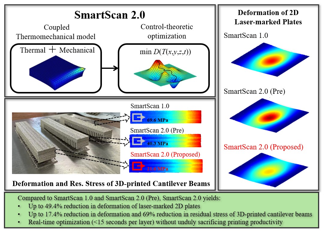
Laser powder bed fusion (LPBF) enables fabrication of complex metal components but remains limited by residual stress accumulation and part deformation. Most existing scan sequence generation strategies for LPBF rely on heuristic rules or empirical optimizations that are suboptimal, difficult to generalize across geometries, and insensitive to the underlying physics of the problem. The SmartScan framework was developed to overcome these limitations through model-based and optimization-driven scan sequence generation. SmartScan 1.0 employed a thermal model to optimize temperature uniformity, leading to significant reductions in residual stress and distortion compared to state-of-the-art heuristic approaches. However, its formulation ignored the mechanical aspects of residual stress and deformation. To address this deficiency, a preliminary study introduced SmartScan 2.0 (Pre) which utilized a decoupled linear thermomechanical formulation for scan sequence optimization for 2D geometries. Building on this foundation, this paper proposes SmartScan 2.0 based on a sequentially coupled linear thermoelastic model that simultaneously solves temperature and displacement fields to minimize thermally induced elastic deformation in 3D geometries. The computational efficiency of SmartScan 2.0 is enhanced through nondimensional scaling. Experimental validation on 3D LPBF specimens shows that SmartScan 2.0 achieves up to 69.0% reduction in residual stress and 17.4% reduction in deformation relative to SmartScan 1.0, and up to 60.6% reduction in residual stress and 12.8% reduction in deformation compared with SmartScan 2.0 (Pre). This work establishes the superiority of scan sequence optimization using coupled linear thermomechanical models over the existing thermal-only or decoupled thermomechanical approaches, without significantly sacrificing computational efficiency.
Keywords:
additive manufacturing
; laser powder bed fusion
; scan strategy
; thermo-mechanical model
; residual stress
; distortion minimization
1. Introduction
Laser powder bed fusion (LPBF) is a core metal additive manufacturing process used across aerospace, automotive, biomedical, and other applications. It uses a high-intensity laser to selectively fuse layers of metal powder to build 3D geometries [1,2]. Despite its ability to form complex parts with high precision and density, LPBF often produces components with residual stress, distortion, cracks, and related defects. These issues arise from the severe thermal environment inherent to the process, including nonuniform heat input, localized heat accumulation, steep temperature gradients, and rapid cooling, which together drive complex thermo-mechanical interactions [3,4,5,6,7,8]. Post-build heat treatments can mitigate residual stress. However, they add cost and time and do not fully remove as-built defects such as distortion and cracking [8,9,10,11]. Consequently, controlling temperature and stress during fabrication, and reducing residual stress and distortion as they form, is critical to ensuring final part quality [12,13].
Scan strategy is central to managing thermal conditions and limiting defects in LPBF. Many studies optimize scan-related parameters such as laser power [14,15,16,17,18], scan speed [18,19,20], layer thickness [21], and scan pattern [7,18,22,23,24]. These efforts have advanced local process control. Scan sequence is another important aspect of scan strategy. It specifies the order in which the laser visits repeating geometric units (features) defined by a chosen scan pattern. Examples include the order of line segments within parallel hatch lines, the order of islands in a chessboard pattern (see Figure 1), and similar subregions. By reshaping the temporal progression of heat input, scan sequence strongly affects thermal history [25], residual stress [26], and part distortion [27] in LPBF components.
Most existing methods for generating scan sequences are heuristic or empirical. They typically rely on simple rules or optimization schemes that approximate heat transfer using geometric relations among features (e.g., the distance between features) [25,26,28,29,30,31]. Common examples include random island, successive island, and successive chessboard sequences. Mugwagwa et al. [26] showed that the successive chessboard sequence reduced average residual stress by up to 40% relative to a random island sequence. Kruth et al. [25] developed a geometry-driven scan sequence called least heat influence (LHI) that chose the next island farthest from previously scanned regions to limit local heat buildup. Later work by Qin et al. [31] refined island ordering with the goal of improving heat uniformity across the layer. These and other similar approaches show measurable benefits in reducing residual stress and, in some cases, distortion compared to less sophisticated scan sequences. Despite these gains, geometry-based methods remain limited because they are blind to the underlying thermomechanical dynamics of LPBF, relying on static geometric proxies instead [25,28,31]. As a result, they are difficult to generalize across parts, materials, and scan patterns, frequently requiring case-specific tuning or retraining, e.g., [25,26,28,29].
These limitations motivated the introduction of the SmartScan framework which aims to generate scan sequences using physics-based (or data-driven) models and control-theoretic optimization [32,33,34,35,36,37,38,39]. The first attempts at SmartScan (herein called SmartScan 1.0) used a physics-based thermal model to optimize temperature uniformity in LPBF [32,33,34,35,36,37,38]. In several studies, SmartScan 1.0 was shown to outperform state-of-the-art heuristic patterns by reducing temperature gradients, residual stress, and/or deformation. For example, in [37], it decreased temperature inhomogeneity by up to 92%, residual stress by 86%, maximum deformation by 24%, and geometric inaccuracies by 50% relative to state-of-the-art heuristic sequences when tested on 3D geometries. It also maintained computational efficiency compatible with real-time use, and it has been implemented in industrial practice as a plug-in to a commercial slicing software package, enabling successful fabrication of a complex 3D part while preventing catastrophic failure [37]. SmartScan 1.0 has inspired other thermal-model-based optimization approaches, like Reinforced Scan [40], which uses a thermal model coupled with reinforcement learning to optimize scan sequences. With sufficient training, Reinforced Scan can explore a wider search space than SmartScan 1.0 and thus potentially provide better solutions as shown by Qin et al. in [40]. However, the training step in Reinforced Scan is computationally very expensive and time consuming, and it requires retraining for each new geometry or set of process parameters. Both of these limit its practicality and versatility.
Regardless of the approach, a major limitation of thermal-based scan sequence optimization solutions, such as SmartScan 1.0 and Reinforced Scan, is that they neglect the mechanical component of the physics that drives residual stress and deformation in LPBF [40,41,42,43,44]. For example, these methods produce the same optimal scan sequence regardless of the mechanical boundary conditions. To address this limitation, the authors introduced the SmartScan 2.0 framework [39,45]. As illustrated in Figure 2, the overarching goal of SmartScan 2.0 is to employ a linear thermomechanical model and objective function to compute optimal scan sequences for each LPBF layer through computationally efficient, control-theoretic optimization.
A preliminary implementation of this framework - here referred to as SmartScan 2.0 (Pre) - adopted a decoupled linear thermomechanical formulation in which the thermal and mechanical fields were treated separately. Its objective was to minimize local temperature gradients (i.e., in the vicinity of the laser) weighted by local compliance information obtained from a linear finite element mechanical model. This thermomechanical objective was optimized using a computationally efficient control-theoretic procedure similar to that employed in SmartScan 1.0 [39]. Using laser marking experiments on 2D plate geometries, SmartScan 2.0 (Pre) was shown to be responsive to mechanical physics (e.g., boundary conditions) and achieved significant reductions in part distortion relative to SmartScan 1.0 in most cases. However, in some scenarios SmartScan 1.0 outperformed SmartScan 2.0 (Pre); for example, it achieved lower mean deformation in a nontrivial fraction of cases [39], revealing the limitations of the decoupled formulation and the locally defined optimization objective.
To overcome these limitations, we propose an improved and generalized approach that better fulfills the overarching goal of the SmartScan 2.0 framework. For simplicity, we refer to this new approach as SmartScan 2.0 distinguishing it from the preliminary version SmartScan 2.0 (Pre). Specifically, this paper makes the following original contributions:
- It introduces a novel control-theoretic optimization approach for scan sequence generation that minimizes thermally induced elastic deformation across the entire part, layer by layer, based on a sequentially coupled linear thermoelastic model.
- It incorporates a nondimensionalized formulation into the proposed SmartScan 2.0 approach to achieve high computational efficiency and scalability.
- Through 2D metal plate laser marking and 3D cantilever beam printing experimental case studies, it demonstrates substantial reductions in residual stress and deformation using the proposed SmartScan 2.0 compared with SmartScan 1.0 and SmartScan 2.0 (Pre), without sacrificing computational efficiency.
The remainder of this paper is organized as follows. Section 2 presents the sequentially coupled linear thermoelastic model, objective function, and the proposed control-theoretic optimization approach. Section 3 then provides a brief theoretical comparison of SmartScan 2.0 with SmartScan 1.0 and SmartScan 2.0 (Pre), ensuring that their similarities and differences are clear. Section 4 introduces the nondimensionalization strategy, grounded in similarity theory, that enables the computational efficiency and scalability of SmartScan 2.0. Section 5 reports experimental validation results benchmarking SmartScan 2.0 against SmartScan 1.0 and SmartScan 2.0 (Pre). Section 6 concludes the paper and outlines future research directions.
2. Proposed SmartScan 2.0
2.1. Overview
The goal of SmartScan 2.0 is to develop an effective and computationally efficient thermomechanical proxy for solving the inverse problem in LPBF; i.e., determining the optimal process inputs (here, the scan sequence) that yield desired outputs such as minimal residual stress and distortion. A proxy is necessary because this inverse problem is far more challenging than the forward problem of predicting outputs from known inputs. Although high-fidelity thermomechanical models capable of accurately predicting residual stress and distortion exist [46,47,48,49], they are too computationally intensive to be practical for inverse optimization, particularly in scan sequence optimization, where the number of possible sequences grows factorially with the number of features in a layer.
To enable tractable optimization, SmartScan 2.0 adopts a linear thermomechanical formulation and therefore does not explicitly model nonlinearities such as strong temperature dependence of material properties, plasticity, or creep. The resulting linear thermoelastic model serves as a simplified but physics-based representation of the process. As a proxy for reducing residual stress and distortion using the simplified model, the optimization targets the minimization of thermally induced elastic deformation during printing. The underlying rationale is that residual stress and distortion arise from plastic deformation, which occurs when thermally induced elastic deformation generates stresses that exceed the yield strength. Therefore, minimizing elastic deformation increases the likelihood of reducing the regions and extent where yielding occurs and, in turn, reducing the magnitude of residual stress and distortion. While this proxy is approximate, as we will show, it provides an effective and computationally efficient alternative to the thermal-only proxies used in prior work. The remainder of this section details the linear thermoelastic model, the resulting objective function, and how these enable an elegant control-theoretic solution for real-time scan sequence optimization.
2.2. Thermal Model
The thermal model is adopted from our prior work on SmartScan 1.0 [37,39]. The model accounts for conductive and convective heat transfer within the part and between the part and its surroundings, while incorporating several simplifying assumptions. In particular, we neglect radiative heat transfer, latent heat effects, Marangoni convection, and other melt pool phenomena [50,51]. We also assume temperature-independent material parameters, yielding a linear model that facilitates efficient optimization. Under these assumptions, heat transfer within the printed part, characterized by conductivity and diffusivity , is governed by the equation:
where T represents temperature, are the spatial coordinates, t is time, and u denotes the power per unit volume. The equation can be discretized using the finite difference method (FDM) with discrete grid sizes , , and an explicit time step to yield:
where are spatial indices for the elements, and l represents the temporal index. The temperature at position and time step l is denoted as . The simplified FDM thermal model, which includes convection boundary conditions on the upper surface of the part (details in Ref. [37]), can be written as a state equation:
where is the temperature vector containing the temperatures of all elements and the constant ambient temperature at time step l, is the state matrix, is the input matrix, and represents the power input vector with non-zero values only at the elements actively heated by the laser at time step l. The model incorporates convection to the ambient temperature , with coefficient h, on its top surfaces. Additionally, the substrate is treated as a heat sink at a constant temperature of . The side edges are considered to be insulated, as the thermal conductivity of the metal powder is extremely low and can be neglected. More details about the setup and validation of this model can be found in [37].
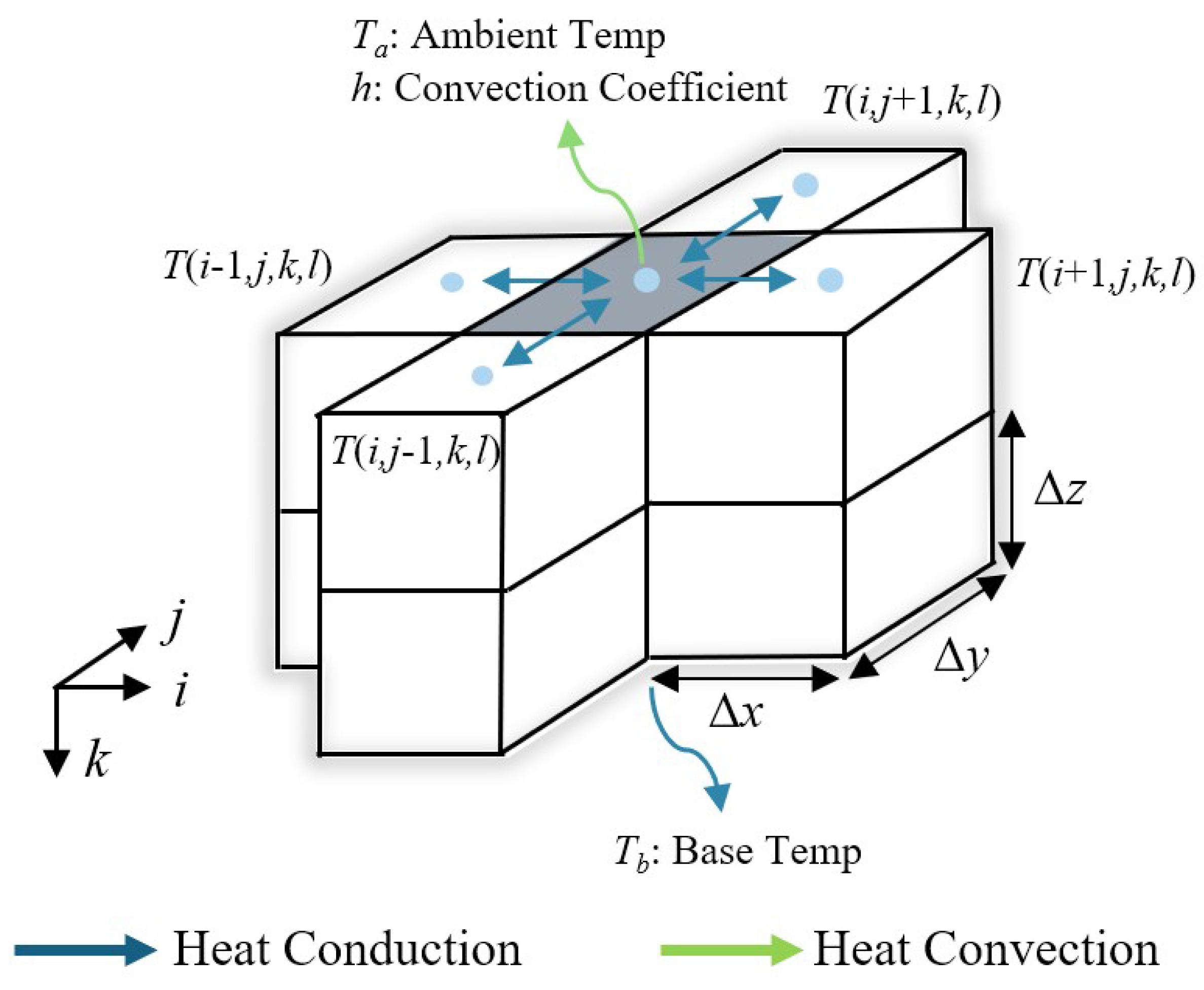
Figure 3.
Simplified thermal finite difference model (FDM) incorporating the assumptions used for SmartScan 2.0, as reported in Ref. [37].
Figure 3.
Simplified thermal finite difference model (FDM) incorporating the assumptions used for SmartScan 2.0, as reported in Ref. [37].
Recall that the features refer to the repeated geometric units in the scan pattern (e.g., vectors or islands). For a total of features, let each feature f require time steps for complete scanning, with its time steps recorded in a set . When scanning each feature , the temperature at any time point where can be expressed as:
where denotes the start time of scanning feature f, and m is the number of time steps that have elapsed at the point of interest. Note that the thermal model assumes zero transition time between consecutive scanned features for simplicity. This assumption is reasonable, as the jump speed is typically much larger than the scanning speed.
2.3. Mechanical Model
In this section, we provide a comprehensive mathematical derivation for addressing pure linear elastic deformation caused by a thermal field, employing the finite element method (FEM). We consider a quasi-static problem where deformation results exclusively from temperature variations, as derived from the calculations in Section 2.2, without any external mechanical loads. The temperature field is represented as a nodal vector , and our objective is to determine the corresponding displacement field .
The linear thermoelastic problem is described by the equilibrium equation [52], assuming no body forces are present:
where represents the stress tensor. For isotropic linear elastic materials that account for thermal effects, the constitutive relationship is given by:
where is the elasticity matrix, which connects stress to strain for the material, is the total strain tensor, and is the thermal strain tensor. In this expression, denotes the coefficient of thermal expansion, denotes the temperature change relative to the reference temperature , and denotes the identity tensor.
The kinematic relationship, which relates the strain tensor to the displacement field , can be expressed as:
where is the displacement gradient tensor.
In FEM, the three-dimensional domain is discretized into a mesh of finite elements. For simplicity, this study uses 8-node hexahedral elements [53] that align with the grid described in Section 2.2. The principle of virtual work is applied to derive the weak form of the thermoelastic problem [54], expressed as:
where represents the virtual strain field and denotes the differential volume element. This formulation assumes no external mechanical loads are applied. By discretizing the domain and assembling contributions from all elements, the global system of equations is obtained as:
with the global stiffness matrix , where the element stiffness matrix is , and the global thermal load vector , where the element thermal load vector is . Additionally, is the finite-element strain–displacement matrix derived from the element shape functions. This study employs the classic trilinear shape functions for 8-node hexahedral elements [53]. For isotropic materials in three-dimensional space, the thermal strain is defined as , where denotes the temperature change in element e relative to the reference temperature , and is the vector accounting for thermal strain components.
With the global nodal temperature change , where , taken as , denotes the initial nodal temperature at the start of scanning for each layer, and assuming that is zero at the initial point, we define the thermal load matrix such that . At the element level, can be expressed as:
Upon global assembly, . At time point , can be represented as
Assuming that is invertible (as ensured by boundary conditions, such as fixed displacements on portions of the boundary ), can be solved through
where . Boundary conditions are applied by modifying , for example, through row and column elimination or penalty methods [55].
2.4. Objective Function and Optimization
SmartScan 2.0 identifies the optimal scanning sequence, ensuring that each feature is scanned exactly once. The objective is to minimize the norm of the elastic deformation vector , which represents the deformation field of the entire part just after the scanning of feature f within each layer is completed, as calculated in Equation (12). Since is a fixed constant, it can be omitted from the objective function to simplify the optimization. Accordingly, the objective function for SmartScan 2.0 (called the elastic deformation metric) can be represented as:
Based on the feature-level state-space representation provided in Equation (4) and the elastic deformation metric defined in Equation (12), the optimization problem applied to the layer of interest can be formulated as follows:
The optimization problem presented in Equation(14) can be reformulated as follows:
Accordingly, the problem is expressed as:
where , , and can be precomputed for each feature in a layer. The feature that minimizes the elastic deformation metric can thus be calculated as the index corresponding to the smallest element in the vector . Figure 4 shows the SmartScan 2.0 optimization workflow. Note that key parameters listed at the top of the flowchart, e.g., the stiffness matrix K, need to be updated after every layer of the optimization, as the part is built.
3. Theoretical Comparison of SmartScan 2.0 to SmartScan 1.0 and 2.0 (Pre)
3.1. Comparison with SmartScan 1.0
SmartScan 1.0 uses the thermal model introduced in Sec. 2.2 (Equation (4)) and optimizes thermal uniformity measured by the thermal uniformity metric, [32,37], defined as
where is the average of the temperature vector over all nodes of the layer being scanned, at time index . Note that is the melting temperature used for normalization.
At each feature-selection step within a layer, SmartScan 1.0 chooses the next feature to minimize , following a solution process that is very similar to that of SmartScan 2.0, as detailed in [37]. Therefore, the fundamental difference between the methods is that SmartScan 1.0 performs scan sequence optimization using a thermal-only objective function and a thermal-only model, while SmartScan 2.0 uses a thermomechanical objective function and model.
3.2. Comparison with SmartScan 2.0 (Pre)
SmartScan 2.0 (Pre) employs a thermomechanical objective function given by:
where refers to the thermal indicator that quantifies the local temperature gradient in the vicinity of the laser and is defined by the norm of the temperature gradient
which is computed from the thermal model in Sec. 2.2. A centered difference implementation gives the discrete form
The mechanical indicator acts as a weight on that emphasizes more compliant regions over stiffer regions. It is derived from the linear elastic finite element model in Sec 2.3 by forming the global stiffness matrix and its compliance , so that higher corresponds to higher compliance. This heuristic weighting is motivated by observations in laser forming: initiating scans in more compliant (less constrained) regions tends to reduce distortion relative to starting near constraints; thus, compliant regions should carry higher weight [56,57]. With these definitions, the objective in Equation( (18)) is an -type objective, sum of absolute temperature gradient components weighted by mechanical compliance. A compact matrix form is
where encodes the discrete gradient operator that extracts the local gradient at the laser location, and contains the normalized mechanical weights along the path of feature f. The resulting selection problem
is solved in essentially the same precomputation accelerated manner as our SmartScan 2.0 formulation (see algorithmic details in [39]).
The key differences of SmartScan 2.0 (Pre) relative to SmartScan 2.0 are: (i) Heuristic vs. non-heuristic objective: SmartScan 2.0 (Pre) uses a thermomechanical objective whose mechanical component is heuristic (compliance-based weighting of a thermal indicator), whereas SmartScan 2.0 in this paper derives a non-heuristic, coupled thermomechanical objective. (ii) Localized vs. part-scale objective: the SmartScan 2.0 (Pre) objective is localized (it focuses on the local temperature gradient at the laser point and the local compliance) while SmartScan 2.0 optimizes over the part scale. (iii) Decoupled vs. coupled thermomechanical formulation: the SmartScan 2.0 (Pre) formulation is decoupled (thermal and mechanical fields are solved separately and combined only through indices in ) whereas SmartScan 2.0 sequentially couples temperature and displacement fields as described in Secs. 2.2 and 2.3.
4. Nondimensionalization of SmartScan 2.0 for Large-Scale Models
Similarity theory offers a rigorous way to scale large thermomechanical systems while preserving essential behavior [58,59,60]. By constructing a reduced, dimensionless model that reproduces the dominant dynamics of the full system, computational cost that would otherwise grow with spatial size (from ) can be made effectively size-independent (approaching ). The approach proceeds by nondimensionalizing the governing equations and ensuring that the resulting dimensionless forms match between the physical and scaled models when the key similarity parameters are equal. In what follows, we apply similarity theory to the sequentially coupled thermomechanical model used in SmartScan 2.0.
We introduce characteristic scales that capture the relevant physics. Let ℓ denote a characteristic length (e.g., a domain dimension), a characteristic temperature difference (e.g., relative to a reference or melting temperature), the thermal diffusion time scale, and Q a characteristic volumetric heat generation rate. For mechanics, we select the displacement scale to reflect thermal expansion, and the stress scale , where E is the Young’s modulus. The dimensionless variables are then
Substituting Equation ((23)) into the heat equation in Equation (1) yields
and, dividing through by , the dimensionless form
where , , , and denote the dimensionless position, temperature, time, and heat-generation term, respectively.
For mechanics, substituting Equation ((23)) into the strain–displacement relation in Equation (7) gives
the constitutive law in Equation (6) becomes
and the equilibrium equation in Equation (5) takes the form
Here, , , and are the dimensionless displacement, strain, and stress. To ensure that a scaled model reproduces the behavior of a larger system, geometric similarity must hold; boundary and initial conditions must be nondimensionalized consistently; and the dimensionless parameters and material properties must match between models. Stability conditions for explicit time stepping in linear thermoelastic systems that couple diffusion and wave propagation are discussed in Ref. [61].
5. Experimental Validation
5.1. Setup of the Experiments
This section evaluates the effectiveness of SmartScan 2.0 introduced in Section 2.4, in direct comparison with SmartScan 1.0 [37] and SmartScan 2.0 (Pre) [39], using two case studies described below. For the sake of brevity, we do not include heuristic scan sequences as benchmarks, because our prior work, and work by others, have shown that SmartScan 1.0 provides substantially greater reductions in part deformation and residual stress than heuristic sequences [31,32,37].
5.1.1. Case Study 1 (Laser Marking of Metal Plates, 2D)
Laser marking experiments were conducted on AISI 316L stainless-steel sheet ( thick; cold-worked and annealed; product no. 88885K11) sourced from McMaster-Carr (Elmhurst, IL, USA). Square plates of size were waterjet cut for testing. The top surface was scanned using an island scan pattern: the plate was partitioned into 100 islands, each ; within each island, 25 bidirectional hatch vectors with spacing were applied, and the scan orientation alternated by between neighboring islands (Figure 1(b)). Material properties and laser parameters used in the optimization and in the experiments are listed in Table 1. Convection boundary conditions were applied to the top and bottom surfaces of the plate, and the side faces were treated as adiabatic due to their small area. Although Table 1 lists a jump speed, the simulations assume instantaneous repositioning because the jump speed is much higher than the mark speed. A dimensionless linear thermoelastic model (Sec. 4) was discretized on a uniform Cartesian grid with explicit time stepping, using nondimensional spacings listed in Table 1. Note that stability for 3D problems requires the satisfaction of: (i) the elastic Courant–Friedrichs–Lewy (CFL) condition [62] and (ii) the thermal Forward-Time Central-Space (FTCS) condition [63]. Both conditions are satisfied for these choices; therefore, the sequentially explicit thermoelastic scheme is stable in three dimensions for the values of , , , and listed in Table 1.
Two sets of mechanical constraints were evaluated for Case Study 1: (i) fully fixed left and right edges (Figure 5(a)) and (ii) fully fixed left and bottom edges (Figure 5(b)). For each constraint set, we compared SmartScan 1.0, SmartScan 2.0 (Pre), and SmartScan 2.0, and we analyzed our primary thermal and thermomechanical objective functions (namely and ) along with the simulated temperature fields and elastic deformation fields, as well as the computation costs of the methods.
Experiments used an open-architecture PANDA 11 (See Figure 6(a)) laser powder bed fusion (LPBF) system (OpenAdditive, LLC, Beavercreek, OH) equipped with a IPG Photonics fiber laser and a varioSCAN system. The system ran on the machine’s Open Machine Control software, which enabled custom scan paths and sequences. Each plate was mounted in a 3D-printed PLA frame (thermal conductivity ) to reduce conductive heat transfer to the build plate and to match the simulation boundary conditions. The plate’s edges were secured with 304 stainless-steel C-clamps, and protective pads limited local contact stress to prevent clamp-induced deformation (Figure 6(b) and (c)). After completing the specified scan for each method, the top-surface deformation was measured with a Romer Absolute Arm 3D scanner (Hexagon, Stockholm, Sweden; model 7525SI; volumetric accuracy ; point repeatability ) before and after being unclamped. The acquired point clouds were processed in MATLAB; the z-coordinate at each point was defined relative to the initial undeformed plane, and MATLAB was used to compute and plot the resulting deformation field.
5.1.2. Case Study 2 (Additive Manufacturing of a Cantilever Beam, 3D)
Three cantilever beams (Figure 7) were printed to compare optimized scan sequences, part distortion, and residual stress across SmartScan 2.0, SmartScan 1.0, and SmartScan 2.0 (Pre). The build time for each method was also recorded. Gas-atomized 316L stainless-steel powder was used (Carpenter Additive, AL), with particle-size distribution –, –, and –. The thermomechanical model configuration for optimization matched Case Study 1 and adopted the following key assumptions (detailed in Ref. [37]): The powder is assumed to act as an effective thermal insulator, with conductivity about one order of magnitude lower than the solid [64]. Because the powder layer is very thin (20–) [65], intra-layer conductivity variation is negligible, and macro-scale heat flow is dominated by conduction into the underlying printed part and substrate, with convective loss at the top surface of the part. Accordingly, the powder layer is omitted from the domain and laser heat input is applied directly to the solid beneath it. The employed material properties and laser settings are listed in Table 1. In contrast to Case Study 1, the hatch spacing was to satisfy the machine-specific processing window for this material. Each layer was hatched with bidirectional scan vectors, and the hatch orientation was rotated by between adjacent layers. The support structures under the beam were included in the optimization domain and represented in both the thermal model and the structural stiffness matrices.
Experiments used the open-architecture PANDA 11 LPBF system described above. A nitrogen cross-flow (along the y-direction in Figure 7) of was maintained. The parts were built without preheating on a stainless-steel baseplate measuring .
5.2. Results and Discussion
5.2.1. Case Study 1 (Laser Marking of Metal Plates, 2D)
Evaluation of Optimized Scan Sequence: The scan sequences produced by the three SmartScan variants under an island pattern with the left and right edges fully constrained (Figure 5(a)) are shown in Figure 8(a). SmartScan 1.0 distributes heat by jumping between islands across the plate to promote thermal uniformity. SmartScan 2.0 (Pre) instead follows a predominantly center-to-edge path: it starts near the more-compliant plate center and progresses towards the stiffer clamped edges while adding pre- and post-heating at the scan frontier to reduce local thermal gradients. In contrast, SmartScan 2.0 combines the global temperature-balancing behavior of SmartScan 1.0 with the boundary-awareness of SmartScan 2.0 (Pre). As a result, it maintains a tendency to move from more to less compliant areas without overly sacrificing plate-wide temperature uniformity.
Optimization results for the island pattern with the left and bottom edges fully constrained (Figure 5(b)) are shown in Figure 8(b). SmartScan 1.0 reproduces the same pattern as in Figure 8(a) because it ignores mechanical boundary conditions and optimizes only the thermal field. SmartScan 2.0 (Pre) produces a sequence that progresses from the more-compliant top-right corner towards the stiffer bottom-left of the plate, again inserting pre- and post-heating at the scan front. SmartScan 2.0 integrates these advantages by seeking global temperature uniformity while accounting for boundary constraints.
Evaluation of Temperature Uniformity Metric and the Temperature Field: In terms of the thermal uniformity metric defined in Equation (17), under the boundary conditions shown in Figure 5(a) SmartScan 1.0 achieves a 16.7% reduction in the mean relative to SmartScan 2.0 (Pre) and a 10.7% reduction relative to SmartScan 2.0. Similarly, under the boundary conditions in Figure 5(b), SmartScan 1.0 shows improvements of 61.5% and 37.5% compared with SmartScan 2.0 (Pre) and SmartScan 2.0, respectively, as presented in Figure 9. These gains are consistent with the simulated dimensionless temperature distributions in Figure 10, which indicate that SmartScan 1.0 prioritizes global temperature uniformity. The fact that SmartScan 1.0 outperforms the other two methods in terms of thermal uniformity is to be expected, since that is the focus of its optimization. However, it is remarkable that SmartScan 2.0, on average, consistently outperforms SmartScan 2.0 (Pre) in thermal uniformity for both boundary conditions. This confirms that the SmartScan 2.0 sequence shown in Figure 8 retains attention to global temperature balancing while incorporating boundary condition awareness.
Evaluation of Elastic Deformation Metric and the Elastic Deformation Field: In terms of the elastic-deformation metric defined in Equation (13), under the boundary conditions shown in Figure 5(a), SmartScan 2.0 achieves a 33.3% reduction in the mean relative to SmartScan 2.0 (Pre) and a 33.3% reduction relative to SmartScan 1.0. Similarly, under the boundary conditions in Figure 5(b), SmartScan 2.0 shows improvements of 33.3% and 20.0% compared with SmartScan 2.0 (Pre) and SmartScan 1.0, respectively, as presented in Figure 11. These gains are consistent with the simulated elastic-deformation field in Figure 12, quantified at each node as the norm of the x-, y-, and z-direction displacements. The results indicate that SmartScan 2.0 prioritizes global minimization of elastic deformation. They also demonstrate that global temperature uniformity does not necessarily yield minimal elastic deformation.
Remark 1
Figure 10 and Figure 12 plot dimensionless temperature and displacement on a scale, consistent with the nondimensional model. This emphasizes relative behavior, which is more relevant to SmartScan, rather than absolute magnitudes.
Evaluation of Metal Plate Deformation: Experimental validation considered the three SmartScan variants used to generate the optimized scan sequences (Figure 8(a)). Figure 13(a) reports the measured out-of-plane deformation profiles under the first boundary condition when the plates remained clamped. The horizontal reference plane is the plate’s initial, undeformed surface. Relative to SmartScan 1.0 and SmartScan 2.0 (Pre), SmartScan 2.0 reduced the maximum deformation by 23.9% and 30.9%, respectively, and reduced the mean deformation by 49.0% and 31.1%, respectively. Under the second boundary condition, the same three strategies were evaluated (Figure 8(b)). Figure 13(b) shows the measured out-of-plane deformation. Compared with SmartScan 1.0 and SmartScan 2.0 (Pre), SmartScan 2.0 lowered the maximum deformation by 24.4% and 16.6%, and lowered the mean deformation by 35.1% and 37.3%, respectively. Both sets of measurements agree with the optimization results, which predicted that SmartScan 2.0 consistently lowers elastic deflection during processing thereby reducing the potential for plastic deformation. It is noteworthy that SmartScan 2.0 (Pre) does not demonstrate a consistent improvement over SmartScan 1.0 in maximum and mean deformation, and observation that is consistent with our prior work [39]. These results indicate that the global temperature uniformity objective used by SmartScan 1.0 and the weighted thermomechanical objective used by SmartScan 2.0 (Pre) are less effective proxies for mitigating part deformation compared to the elastic deformation metric used by SmartScan 2.0.
Figure 14 reports the deformation of the metal plates after removal from the clamps. In Figure 14(a), we show the measured out-of-plane deformation under the first boundary condition. Heights are referenced to a horizontal datum plane defined by the table surface on which the plates were placed during 3D scanning. For the first boundary condition, relative to SmartScan 1.0 and SmartScan 2.0 (Pre), SmartScan 2.0 reduced the maximum deformation by 23.8% and 30.7%, respectively, and reduced the mean deformation by 33.8% and 49.4%, respectively. Under the second boundary condition, the same three strategies were evaluated (Figure 14(b)). Compared with SmartScan 1.0 and SmartScan 2.0 (Pre), SmartScan 2.0 lowered the maximum deformation by 24.1% and 16.5%, and lowered the mean deformation by 29.9% and 42.1%, respectively. These results are consistent with the overarching observations made regarding the unclamped plates.
Evaluation of Computing Time for Computation: Computational efficiency is essential for real time deployment. In LPBF, the per-layer optimization must be completed within the interlayer dwell when powder is recoated, to achieve real-time optimization. Prior results for SmartScan 1.0 report per-layer runtimes below , which fall within typical interlayer durations [37]. As summarized in Table 2, all SmartScan variants satisfy this criterion across all test cases, meeting the real time requirement. All computations were performed on a workstation with an AMD Ryzen 9 7945HX CPU, RAM, and an NVIDIA GeForce RTX 4070 Laptop GPU.
5.2.2. Case Study 2 (Additive Manufacturing of a Cantilever Beam, 3D)
Evaluation of Optimized Scan Sequences:Figure 15 shows the optimized scan sequences produced by the three SmartScan variants for an arbitrarily selected layer: Layer 150, which contains 680 vertical bidirectional hatch vectors. SmartScan 1.0 yields a sequence with large global jumps, in a bid to maximize thermal uniformity. SmartScan 2.0 (Pre) progresses from the mechanically compliant end towards the stiffer end, producing a predominantly right-to-left traversal with pre- and post- heating at the scan frontier to minimize thermal gradients. SmartScan 2.0 combines the behaviors of SmartScan 1.0 and SmartScan 2.0 (Pre), achieving an integrated trade-off between thermal uniformity and mechanical constraints.
Evaluation of Cantilever Deformation:Figure 16 presents the printed cantilever beams fabricated using three distinct scanning strategies, which were employed to evaluate part distortion and residual stress. To quantify distortion, the thin support structures were cut off from the build plate using a band saw, after which the top surface of each part was scanned using the Romer Absolute Arm described in Section 5.1.1 to extract post-printing deformation. As expected for stress-relief events, the upper surfaces exhibited upward bending upon release, and these deformations were captured as point clouds and subsequently visualized and analyzed in MATLAB. Relative to SmartScan 1.0 and SmartScan 2.0 (Pre), SmartScan 2.0 achieved reductions of 7.9% and 8.5% in the maximum part deflection, and 17.4% and 12.8% in the mean part deflection, respectively. These results are, in general, consistent with those of Case Study 1, and show that SmartScan 2.0 mitigates deformation more effectively than both SmartScan 1.0 and SmartScan 2.0 (Pre).
Evaluation of Residual Stress: Finally, we extracted a specimen that captures most of the solid block on the left side of the cantilever beam in Figure 7 for residual stress measurements. The block was removed from the build plate by electrical discharge machining (EDM) without any observable distortion, so it is expected to retain much of the residual stress accumulated during printing. Residual stress along the x and y directions was measured within a area, highlighted in yellow in Figure 7. A Cu-target X-ray diffractometer (Rigaku Ultima IV XRD) was used, and the instrument’s proprietary PDLX software processed the data. The operating conditions were and . We applied the method with tilt angles , , , , , and for two series of samples. The elastic modulus was fixed at , and the Poisson’s ratio was set to for all analyses. Figure 17 summarizes the residual stress measurements obtained by XRD. Relative to SmartScan 1.0 and SmartScan 2.0 (Pre), SmartScan 2.0 reduces the mean x-direction residual stress by 69.0% and 46.4%, respectively, and reduces the mean y-direction residual stress by 34.6% and 60.6%, respectively. These reductions are practically significant. Lower as-built residual stress reduces the risk of stress-induced build failures even before any post-process stress relief. In tests, SmartScan 2.0 maintained low residual stresses across the build, further decreasing the risk of part failure.
Evaluation of Print Time:Table 3 summarizes the recorded build time for each sample during the experiments. Based on these measurements, SmartScan 2.0 reduced the total print time by 7.8% relative to SmartScan 1.0, primarily by shortening excessive jump motions. This result indicates that SmartScan 2.0 can simultaneously mitigate part distortion and residual stress while also shortening the overall build time compared to SmartScan 1.0. While SmartScan 2.0 (Pre) achieved shorter print time than other strategies, it was not as effective as SmartScan 2.0 in reducing residual stress and distortion.
6. Conclusions and Future Work
This paper has presented SmartScan 2.0, a model-based, optimization driven approach for scan sequence generation in LPBF. Extending the thermal formulation of SmartScan 1.0 [32,37] and the decoupled thermomechanical approach of SmartScan 2.0 (Pre) [39,45], the proposed method employs a coupled thermoelastic model that sequentially resolves temperature and elastic displacement fields. The SmartScan 2.0 formulation is nondimensionalized for scalability and real-time execution.
6.1. Key Conclusions
- SmartScan 2.0 introduces a novel proxy for scan sequence optimization: SmartScan 2.0 introduces the elastic deformation metric as a global objective derived from a sequentially coupled thermoelastic model. This proxy, while highly simplified, is much more sophisticated than heuristic, thermal-only or decoupled thermomechanical proxies used in prior works on scan sequence optimization. It is also sensible. By directly minimizing elastic deformation, it reduces the potential for plastic strain which is the source of residual stress and deformation.
- SmartScan 2.0 is effective in reducing in residual stress and deformation: In 2D laser marking of plates, it reduced maximum and mean out-of-plane deformation by up to 30.7% and 49.4%, respectively, relative to SmartScan 1.0 and SmartScan 2.0 (Pre). In 3D cantilever builds, it achieved reductions of up to 8.5% in maximum deformation and 17.4% in mean deformation, and up to 69.0% in residual stress, compared to SmartScan 1.0 and SmartScan 2.0 (Pre).
- SmartScan 2.0 is computationally efficient and practical: Enabled by its simplified proxy, nondimensionalized modeling, and control-theoretic optimization, SmartScan 2.0 delivers the results discussed above in a computationally efficient manner without sacrificing productivity. Per-layer runtimes remained below 15 s, and total print times matched or modestly improved upon SmartScan 1.0 (7.8% faster in the 3D case). Such efficiency supports real-time implementation and seamless integration into commercial slicing environments, as with SmartScan 1.0 [37].
6.2. Future Work
- Enhanced physical modeling: Work is underway to extend the elastic deformation proxy to account for plasticity and other important nonlinear physics that influence residual stress and deformation. The central challenge will be incorporating these nonlinear effects while preserving computational tractability for inverse optimization.
- Broader validation: Upcoming studies will evaluate SmartScan 2.0’s influence on microstructure, surface roughness, and porosity, and apply it to more complex 3D geometries. Integration into commercial slicers will facilitate such evaluations and accelerate technology transfer to industry.
- Toward closed-loop, multiphysics optimization: Future extensions will explore coupling SmartScan with in-situ sensing (e.g., thermography, melt-pool monitoring) for adaptive process optimization. Combining scan sequence optimization with process parameter tuning (e.g., laser power and speed) could enable a comprehensive, multiphysics optimization framework for intelligent LPBF.
Acknowledgments
We thank Dr. Zhongrui (Jerry) Li for conducting the X-ray diffraction (XRD) residual stress measurements reported here and Dr. Mihaela (Miki) Banu for providing the 3D scanner used to quantify deformation. We also thank Mr. Samuel Thompson and Mr. Yi-Sien Ku for suggestions that led to the nondimensionalized modeling approach used in this work. The authors are grateful to Dr. Tao Liu and Mr. Nicholas Kirschbaum for helpful feedback on the presentation of this work. This work was partially supported by Grant# CMMI 2430109 from the National Science Foundation (NSF).
Conflicts of Interest
The Regents of the University of Michigan have filed a provisional patent related to SmartScan 2.0. SmartScan 1.0 is currently licensed by the Regents of the University of Michigan to a company co-owned by one of the authors.
References
- Chowdhury, S.; Yadaiah, N.; Prakash, C.; Ramakrishna, S.; Dixit, S.; Gupta, L.R.; Buddhi, D. Laser powder bed fusion: a state-of-the-art review of the technology, materials, properties & defects, and numerical modelling. Journal of Materials Research and Technology 2022, 20, 2109–2172. [Google Scholar]
- Kotadia, H.; Gibbons, G.; Das, A.; Howes, P. A review of Laser Powder Bed Fusion Additive Manufacturing of aluminium alloys: Microstructure and properties. Additive Manufacturing 2021, 46, 102155. [Google Scholar] [CrossRef]
- Dong, G.; Wong, J.C.; Lestandi, L.; Mikula, J.; Vastola, G.; Jhon, M.H.; Dao, M.H.; Kizhakkinan, U.; Ford, C.S.; Rosen, D.W. A part-scale, feature-based surrogate model for residual stresses in the laser powder bed fusion process. Journal of Materials Processing Technology 2022, 304, 117541. [Google Scholar] [CrossRef]
- Burgio, V.; Moeini, G. Laser Powder Bed Fusion Additive Manufacturing of a CoCrFeNiCu High-Entropy Alloy: Processability, Microstructural Insights, and (In Situ) Mechanical Behavior. Materials 2025, 18, 3071. [Google Scholar] [CrossRef]
- Wang, W.; Zhang, G.; Yang, B.; Chen, Q.; Yang, Z.; Liu, S.; Dong, F. Study on the Evolution of Deformation Trend in Laser Powder Bed Fusion Samples Based on a Novel Monitoring System. Sensors 2025, 25, 1043. [Google Scholar] [CrossRef]
- Park, H.; Mullin, K.M.; Kumar, V.; Wander, O.; Pollock, T.M.; Zhu, Y. Resolving thermal gradients and solidification velocities during laser melting of a refractory alloy. Additive Manufacturing 2025, 105, 104750. [Google Scholar] [CrossRef]
- Wang, Y.; Chen, C.; Qi, Y.; Zhu, H. Residual stress reduction and surface quality improvement of dual-laser powder bed fusion. Additive Manufacturing 2023, 71, 103565. [Google Scholar] [CrossRef]
- Zhang, R.; Strickland, J.; Hou, X.; Yang, F.; Li, X.; de Oliveira, J.A.; Li, J.; Zhang, S. Rapid residual stress simulation and distortion mitigation in laser additive manufacturing through machine learning. Additive Manufacturing 2025, 102, 104721. [Google Scholar] [CrossRef]
- Chen, Q.; Taylor, H.; Takezawa, A.; Liang, X.; Jimenez, X.; Wicker, R.; To, A.C. Island scanning pattern optimization for residual deformation mitigation in laser powder bed fusion via sequential inherent strain method and sensitivity analysis. Additive Manufacturing 2021, 46, 102116. [Google Scholar] [CrossRef]
- Cao, S.; Zou, Y.; Lim, C.V.S.; Wu, X. Review of laser powder bed fusion (LPBF) fabricated Ti-6Al-4V: process, post-process treatment, microstructure, and property. Light: Advanced Manufacturing 2021, 2, 1. [Google Scholar] [CrossRef]
- Guo, C.; Li, S.; Shi, S.; Li, X.; Hu, X.; Zhu, Q.; Ward, R.M. Effect of processing parameters on surface roughness, porosity and cracking of as-built IN738LC parts fabricated by laser powder bed fusion. Journal of Materials Processing Technology 2020, 285, 116788. [Google Scholar] [CrossRef]
- Kumar, V.P.; Jebaraj, A.V. Comprehensive review on residual stress control strategies in laser-based powder bed fusion process– Challenges and opportunities. Lasers in Manufacturing and Materials Processing 2023, 10, 400–442. [Google Scholar] [CrossRef]
- Narasimharaju, S.R.; Zeng, W.; See, T.L.; Zhu, Z.; Scott, P.; Jiang, X.; Lou, S. A comprehensive review on laser powder bed fusion of steels: Processing, microstructure, defects and control methods, mechanical properties, current challenges and future trends. Journal of Manufacturing Processes 2022, 75, 375–414. [Google Scholar] [CrossRef]
- Reiff, C.; Bubeck, W.; Krawczyk, D.; Steeb, M.; Lechler, A.; Verl, A. Learning Feedforward Control for Laser Powder Bed Fusion. Procedia CIRP 2021, 96, 127–132. [Google Scholar] [CrossRef]
- Riensche, A.; Bevans, B.; Carrington Jr, A.; Deshmukh, K.; Shephard, K.; Sions, J.; Synder, K.; Plotnikov, Y.; Cole, K.; Rao, P. DynamicPrint: A physics-guided feedforward model predictive process control approach for defect mitigation in laser powder bed fusion additive manufacturing. Additive Manufacturing 2025, 97, 104592. [Google Scholar] [CrossRef]
- Wang, R.; Standfield, B.; Dou, C.; Law, A.C.; Kong, Z.J. Real-time process monitoring and closed-loop control on laser power via a customized laser powder bed fusion platform. Additive Manufacturing 2023, 66, 103449. [Google Scholar] [CrossRef]
- Kirschbaum, N.; Wood, N.; Kim, C.E.; Tumkur, T.U.; Okwudire, C. Vector-level feedforward control of LPBF melt pool area using a physics-based thermal model. Additive Manufacturing 2025, 104981. [Google Scholar] [CrossRef]
- Billingham, J.; Yeung, H.; Axinte, D.; Liao, Z.; Fox, J. The inverse heat placement problem in metal additive manufacturing: Why a rational approach is needed for powder bed fusion. Journal of Materials Processing Technology 2024, 329, 118447. [Google Scholar] [CrossRef]
- Ding, L.; Liu, J.; Tan, S.; Zhang, Y.; Fan, C.; Gomes, S.; Zhang, Y. A novel layer-based optimization method for stabilizing the early printing stage of LPBF process. Virtual and Physical Prototyping 2024, 19, e2325578. [Google Scholar] [CrossRef]
- Freitas, B.J.M.; Koga, G.Y.; Arneitz, S.; Bolfarini, C.; de Traglia Amancio-Filho, S. Optimizing LPBF-parameters by Box-Behnken design for printing crack-free and dense high-boron alloyed stainless steel parts. Additive Manufacturing Letters 2024, 9, 100206. [Google Scholar] [CrossRef]
- Liu, T.; Kinzel, E.C.; Leu, M.C. In-situ lock-in thermographic measurement of powder layer thermal diffusivity and thickness in laser powder bed fusion. Additive Manufacturing 2023, 74, 103726. [Google Scholar] [CrossRef]
- Malekipour, E.; Valladares, H.; Shin, Y.; El-Mounayri, H. Optimization of Chessboard Scanning Strategy Using Genetic Algorithm in Multi-Laser Additive Manufacturing Process. American Society of Mechanical Engineers, 11 2020. [CrossRef]
- Kim, S.I.; Hart, A.J. A spiral laser scanning routine for powder bed fusion inspired by natural predator-prey behaviour. Virtual and Physical Prototyping 2022, 17, 239–255. [Google Scholar] [CrossRef]
- Ramani, K.S.; Shrotriya, N. Intelligent Scan Pattern Optimization for Reduced Thermal Gradients in Metal Additive Manufacturing. IFAC-PapersOnLine 2024, 57, 185–189. [Google Scholar] [CrossRef]
- Kruth, J.; Froyen, L.; Vaerenbergh, J.V.; Mercelis, P.; Rombouts, M.; Lauwers, B. Selective laser melting of iron-based powder. Journal of Materials Processing Technology 2004, 149, 616–622. [Google Scholar] [CrossRef]
- Mugwagwa, L.; Dimitrov, D.; Matope, S.; Yadroitsev, I. Evaluation of the impact of scanning strategies on residual stresses in selective laser melting. The International Journal of Advanced Manufacturing Technology 2019, 102, 2441–2450. [Google Scholar] [CrossRef]
- Li, C.; Fu, C.; Guo, Y.; Fang, F. A multiscale modeling approach for fast prediction of part distortion in selective laser melting. Journal of materials processing technology 2016, 229, 703–712. [Google Scholar] [CrossRef]
- Holman, D.; Boseila, J.; Schleifenbaum, J.H. New Island Partitioning to Improve Scanning Strategies in Powder Bed Fusion of Metals with Laser Beam. BHM Berg-und Hüttenmännische Monatshefte 2025, 170, 140–147. [Google Scholar] [CrossRef]
- Liu, Y.; Li, J.; Xu, K.; Cheng, T.; Zhao, D.; Li, W.; Teng, Q.; Wei, Q. An optimized scanning strategy to mitigate excessive heat accumulation caused by short scanning lines in laser powder bed fusion process. Additive Manufacturing 2022, 60, 103256. [Google Scholar] [CrossRef]
- Ramos, D.; Belblidia, F.; Sienz, J. New scanning strategy to reduce warpage in additive manufacturing. Additive Manufacturing 2019, 28, 554–564. [Google Scholar] [CrossRef]
- Qin, M.; Qu, S.; Ding, J.; Song, X.; Gao, S.; Wang, C.C.; Liao, W.H. Adaptive toolpath generation for distortion reduction in laser powder bed fusion process. Additive Manufacturing 2023, 64, 103432. [Google Scholar] [CrossRef]
- Ramani, K.S.; He, C.; Tsai, Y.L.; Okwudire, C.E. SmartScan: An Intelligent Scanning Approach for Uniform Thermal Distribution, Reduced Residual Stresses and Deformations in PBF Additive Manufacturing. Additive Manufacturing, 2022; 102643. [Google Scholar] [CrossRef]
- He, C.; Tsai, Y.L.; Okwudire, C.E. A Comparative Study on the Effects of an Advanced Scan Pattern and Intelligent Scan Sequence on Thermal Distribution, Part Deformation, and Printing Time in PBF Additive Manufacturing. In Proceedings of the Proc. International Manufacturing Science and Engineering Conference; 6 2022. [Google Scholar] [CrossRef]
- He, C.; Ramani, K.S.; Tsai, Y.L.; Okwudire, C.E. A Simplified Scan Sequence Optimization Approach for PBF Additive Manufacturing of Complex Geometries. In Proceedings of the Proc. IEEE/ASME International Conference on Advanced Intelligent Mechatronics (AIM); 7 2022; pp. 1004–1009. [Google Scholar] [CrossRef]
- He, C.; Ramani, K.S.; Okwudire, C.E. An intelligent scanning strategy (SmartScan) for improved part quality in multi-laser PBF additive manufacturing. Additive Manufacturing 2023, 64, 103427. [Google Scholar] [CrossRef]
- He, C.; Okwudire, C. Scan Sequence Optimization for Reduced Residual Stress and Distortion in PBF Additive Manufacturing – An AISI 316L Case Study. In Proceedings of the Proc. Ground Vehicle Systems Engineering and Technology Symposium (GVSETS); 8 2023. [Google Scholar]
- He, C.; Wood, N.; Bugdayci, N.B.; Okwudire, C. Generalized SmartScan: An Intelligent LPBF Scan Sequence Optimization Approach for Reduced Residual Stress and Distortion in Three-Dimensional Part Geometries. Journal of Manufacturing Science and Engineering 2025, 147, 041001. [Google Scholar] [CrossRef]
- Yao, Y.; He, C.; Okwudire, C.; Madhyastha, H.V. Cosmic:{Cost-Effective} Support for {Cloud-Assisted} 3D Printing. In Proceedings of the 2025 USENIX Annual Technical Conference (USENIX ATC 25); 2025; pp. 73–88. [Google Scholar]
- He, C.; Liu, T.; Okwudire, C.E. SmartScan 2.0: an intelligent scan sequence optimization approach for LPBF driven by thermomechanical models. Manufacturing Letters 2025, 44, 1026–1037. [Google Scholar] [CrossRef]
- Qin, M.; Ding, J.; Qu, S.; Song, X.; Wang, C.C.; Liao, W.H. Deep reinforcement learning based toolpath generation for thermal uniformity in laser powder bed fusion process. Additive Manufacturing 2024, 79, 103937. [Google Scholar] [CrossRef]
- Mirkoohi, E.; Tran, H.C.; Lo, Y.L.; Chang, Y.C.; Lin, H.Y.; Liang, S.Y. Analytical modeling of residual stress in laser powder bed fusion considering part’s boundary condition. Crystals 2020, 10, 337. [Google Scholar] [CrossRef]
- Mirkoohi, E.; Tran, H.C.; Lo, Y.L.; Chang, Y.C.; Lin, H.Y.; Liang, S.Y. Mechanics modeling of residual stress considering effect of preheating in laser powder bed fusion. Journal of Manufacturing and Materials Processing 2021, 5, 46. [Google Scholar] [CrossRef]
- Carraturo, M.; Jomo, J.; Kollmannsberger, S.; Reali, A.; Auricchio, F.; Rank, E. Modeling and experimental validation of an immersed thermo-mechanical part-scale analysis for laser powder bed fusion processes. Additive Manufacturing 2020, 36, 101498. [Google Scholar] [CrossRef]
- Zhang, Z.; Wang, Y.; Ge, P.; Wu, T. A review on modelling and simulation of laser additive manufacturing: Heat transfer, microstructure evolutions and mechanical properties. Coatings 2022, 12, 1277. [Google Scholar] [CrossRef]
- He, C.; Okwudire, C. Toward SmartScan 2.0 – An Intelligent Scanning Sequence Optimization Method for Reduced Part Deformation and Residual Stress in LPBF Based on Thermo-Mechanical Models. Conference presentation, 35th Annual International Solid Freeform Fabrication Symposium (SFF 2024), Austin, Texas, USA, August 11–14, 2024.
- Bayraktar, C.; Demir, E. A thermomechanical finite element model and its comparison to inherent strain method for powder-bed fusion process. Additive Manufacturing 2022, 54, 102708. [Google Scholar] [CrossRef]
- Ganeriwala, R.; Strantza, M.; King, W.; Clausen, B.; Phan, T.Q.; Levine, L.E.; Brown, D.W.; Hodge, N. Evaluation of a thermomechanical model for prediction of residual stress during laser powder bed fusion of Ti-6Al-4V. Additive Manufacturing 2019, 27, 489–502. [Google Scholar] [CrossRef]
- Dong, W.; Liang, X.; Chen, Q.; Hinnebusch, S.; Zhou, Z.; To, A.C. A new procedure for implementing the modified inherent strain method with improved accuracy in predicting both residual stress and deformation for laser powder bed fusion. Additive Manufacturing 2021, 47, 102345. [Google Scholar] [CrossRef]
- Chen, Q.; Liang, X.; Hayduke, D.; Liu, J.; Cheng, L.; Oskin, J.; Whitmore, R.; To, A.C. An inherent strain based multiscale modeling framework for simulating part-scale residual deformation for direct metal laser sintering. Additive Manufacturing 2019, 28, 406–418. [Google Scholar] [CrossRef]
- Yavari, R.; Williams, R.; Riensche, A.; Hooper, P.A.; Cole, K.D.; Jacquemetton, L.; Halliday, H.S.; Rao, P.K. Thermal modeling in metal additive manufacturing using graph theory – Application to laser powder bed fusion of a large volume impeller. Additive Manufacturing 2021, 41, 101956. [Google Scholar] [CrossRef]
- Scheel, P.; Markovic, P.; Van Petegem, S.; Makowska, M.G.; Wrobel, R.; Mayer, T.; Leinenbach, C.; Mazza, E.; Hosseini, E. A close look at temperature profiles during laser powder bed fusion using operando X-ray diffraction and finite element simulations. Additive Manufacturing Letters 2023, 6, 100150. [Google Scholar] [CrossRef]
- Boley, B.A.; Weiner, J.H. Theory of thermal stresses; Courier Corporation, 2012.
- Psihoyos, H.; Lampeas, G. Efficient Simulation of the Laser-Based Powder Bed Fusion Process Demonstrated on Open Lattice Materials Fabrication. Machines 2024, 12, 369. [Google Scholar] [CrossRef]
- Chen, J.Z. Finite Element Method, The: Its Fundamentals And Applications In Engineering; World Scientific Publishing Company, 2011.
- Meyer, J.; Kaliske, M. Enforcement of non-conforming dirichlet boundary conditions in the implicit material point method using the direct elimination method. Computational Mechanics 2025, 1–22. [Google Scholar] [CrossRef]
- Birnbaum, A.J.; Cheng, P.; Yao, Y.L. Effects of clamping on the laser forming process. Journal of Manufacturing Science and Engineering 2007, 129, 1035–1044. [Google Scholar] [CrossRef]
- Chen, F.; Zha, R.; Jeong, J.; Liao, S.; Cao, J. Directed energy deposition on sheet metal forming for reinforcement structures. Journal of Manufacturing Processes 2025, 144, 339–349. [Google Scholar] [CrossRef]
- Zuo, Y.; Fu, W.; Xu, P.; Wang, X.; Li, S.; Xu, S.; Wu, H.; Liu, Y.; Xiao, J.; Wang, H. Study on vibration characteristics of large caliber naval gun cradle based on similarity theory. Results in Engineering 2022, 15, 100529. [Google Scholar] [CrossRef]
- Wang, Y.; Wu, T.; Liu, T.; Sha, J.; Ren, H. Numerical simulation and experimental verification of the steady-state heat transfer similarity theory based on dimensional analysis. Case Studies in Thermal Engineering 2024, 60, 104714. [Google Scholar] [CrossRef]
- Pucciarelli, A.; Ambrosini, W. A successful general fluid-to-fluid similarity theory for heat transfer at supercritical pressure. International journal of heat and mass transfer 2020, 159, 120152. [Google Scholar] [CrossRef]
- Li, Z.; Wang, D.; Zou, J. Theoretical and numerical analysis on a thermo-elastic system with discontinuities. Journal of computational and applied mathematics 1998, 92, 37–58. [Google Scholar]
- Bürchner, T.; Radtke, L.; Kopp, P. A CFL condition for the finite cell method. arXiv preprint, 2025; arXiv:2502.13675. [Google Scholar]
- Haque, M.N.; Akter, R.; Mojumder, M.S.H. An Efficient Explicit Scheme for Solving the 2D Heat Equation with Stability and Convergence Analysis. Journal of Applied Mathematics and Physics 2025, 13, 2234–2244. [Google Scholar] [CrossRef]
- Wei, L.C.; Ehrlich, L.E.; Powell-Palm, M.J.; Montgomery, C.; Beuth, J.; Malen, J.A. Thermal conductivity of metal powders for powder bed additive manufacturing. Additive Manufacturing 2018, 21, 201–208. [Google Scholar] [CrossRef]
- Mahmoodkhani, Y.; Ali, U.; Shahabad, S.I.; Kasinathan, A.R.; Esmaeilizadeh, R.; Keshavarzkermani, A.; Marzbanrad, E.; Toyserkani, E. On the measurement of effective powder layer thickness in laser powder-bed fusion additive manufacturing of metals. Progress in Additive Manufacturing 2019, 4, 109–116. [Google Scholar] [CrossRef]
Figure 1.
Example of two common scan patterns in LPBF: (a) the vector pattern, which uses parallel scan lines, and (b) the island pattern, which divides the build area into small squares. Scan sequence determines the order in which these features (e.g., vectors or islands, as marked by the red boxes) are processed.
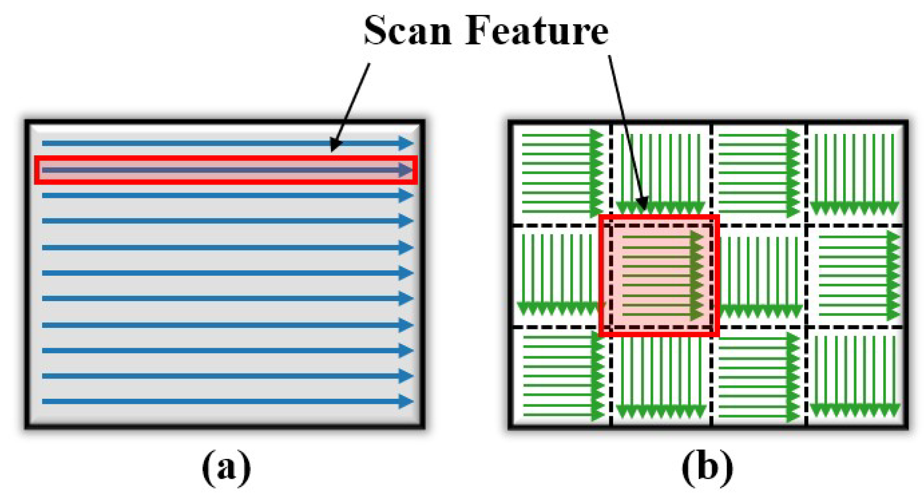
Figure 2.
Flowchart of SmartScan 2.0: an intelligent scan sequence optimization framework based on a linear thermomechanical model.
Figure 2.
Flowchart of SmartScan 2.0: an intelligent scan sequence optimization framework based on a linear thermomechanical model.
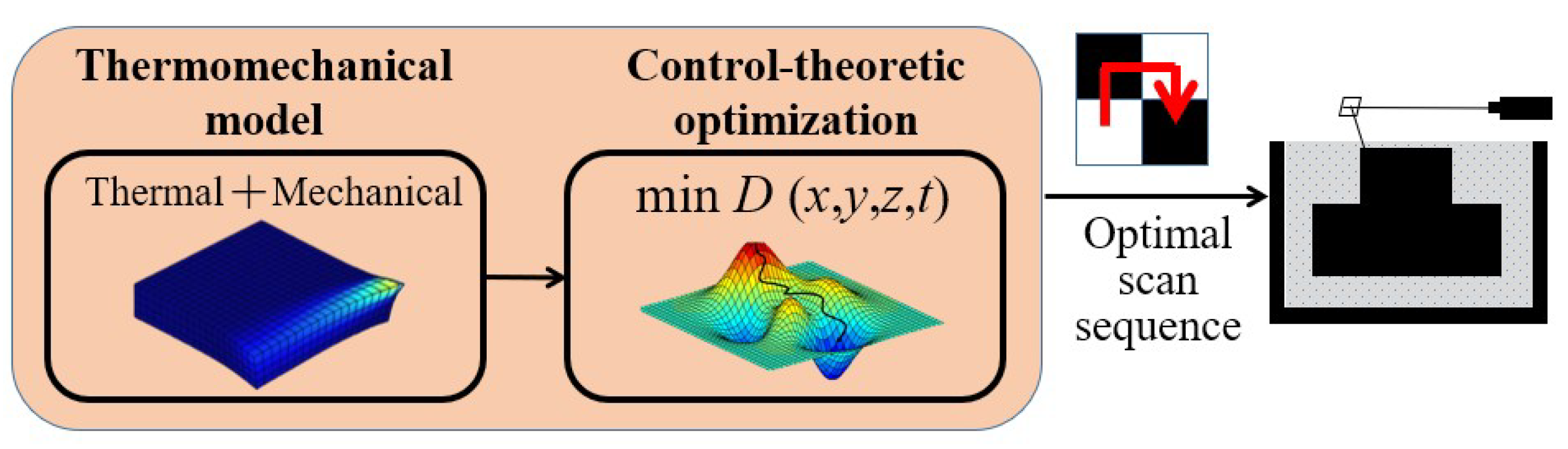
Figure 4.
SmartScan 2.0 optimization workflow.
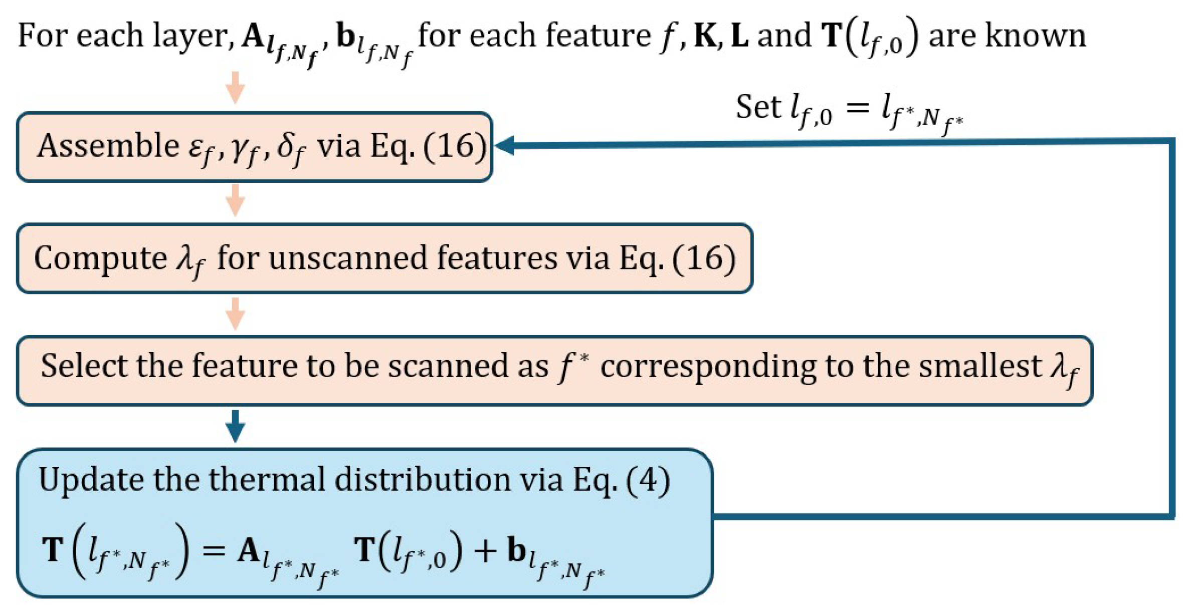
Figure 5.
Case study 1 with island scan patterns under two boundary constraints: (a) fixed left and right edges, and (b) fixed left and bottom edges.
Figure 5.
Case study 1 with island scan patterns under two boundary constraints: (a) fixed left and right edges, and (b) fixed left and bottom edges.
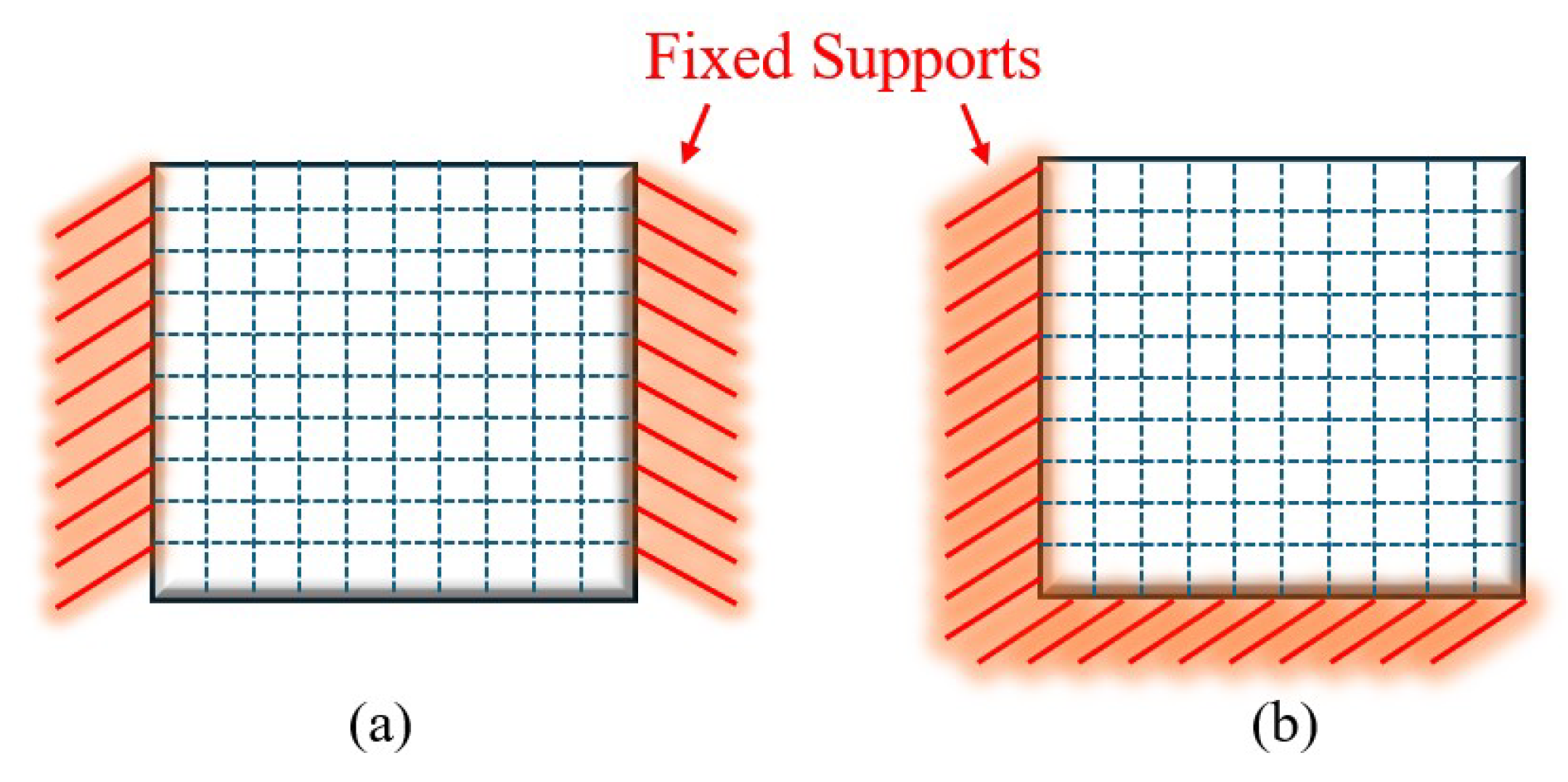
Figure 6.
(a) PANDA 11 open-architecture LPBF machine. Fixture configurations used to impose (b) fully fixed left and right edges and (c) fully fixed left and bottom edges. The clamping grooves are shallow with depth .
Figure 6.
(a) PANDA 11 open-architecture LPBF machine. Fixture configurations used to impose (b) fully fixed left and right edges and (c) fully fixed left and bottom edges. The clamping grooves are shallow with depth .
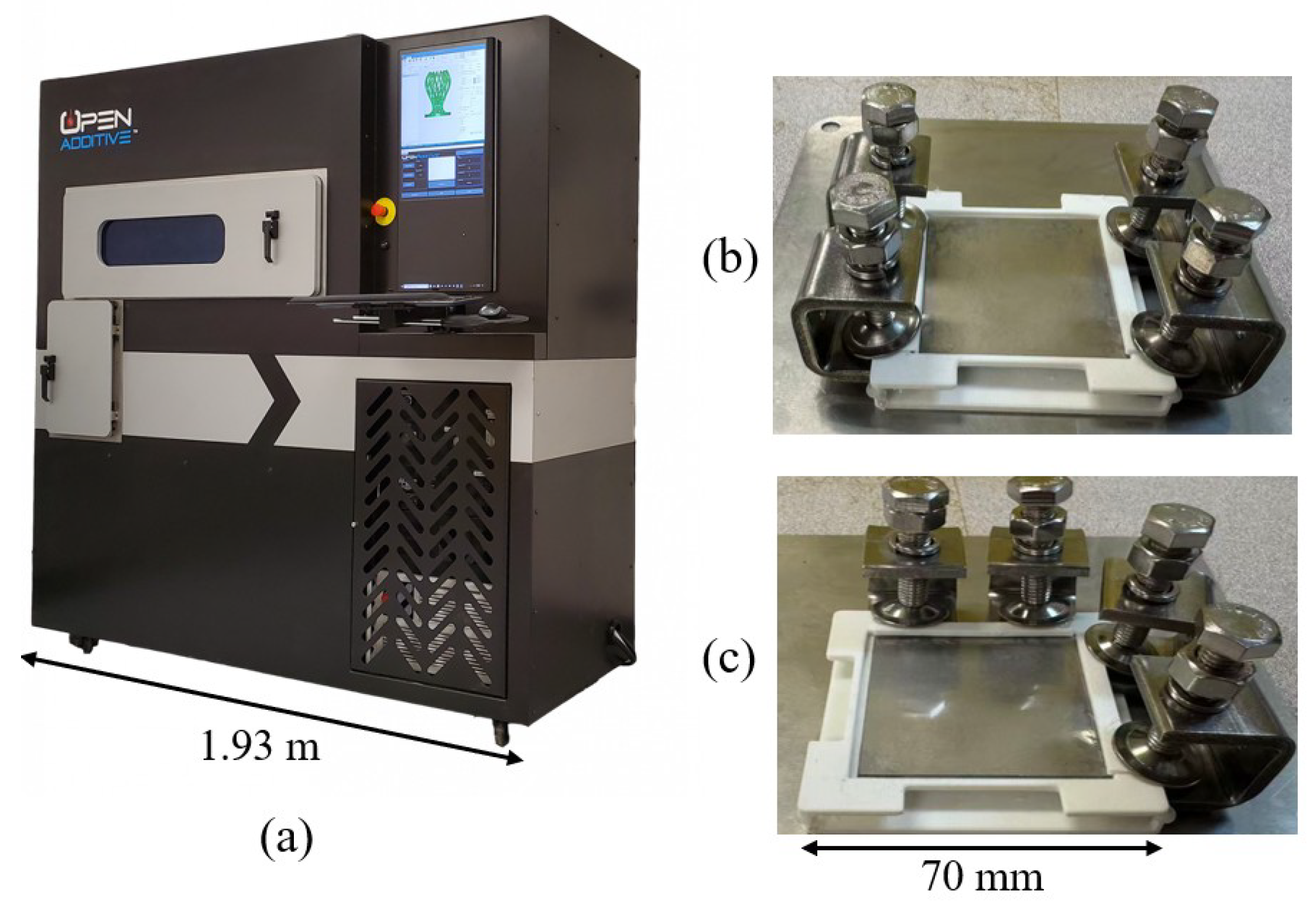
Figure 7.
Cantilever-beam geometry employed in the simulations and experiments for Case Study 2.
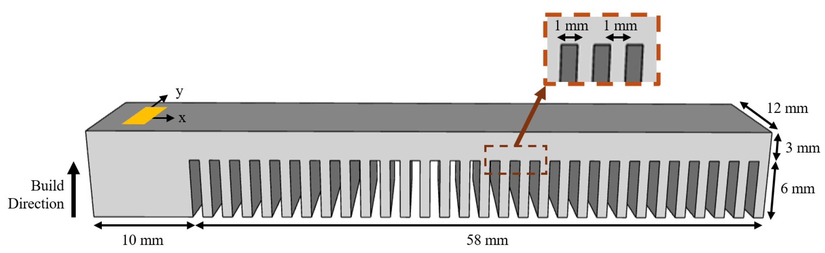
Figure 8.
Numbered color maps comparing scan sequences for SmartScan 1.0, SmartScan 2.0 (Pre), and SmartScan 2.0 under the island pattern, with (a) left and right edges fixed and (b) left and bottom edges fixed.
Figure 8.
Numbered color maps comparing scan sequences for SmartScan 1.0, SmartScan 2.0 (Pre), and SmartScan 2.0 under the island pattern, with (a) left and right edges fixed and (b) left and bottom edges fixed.
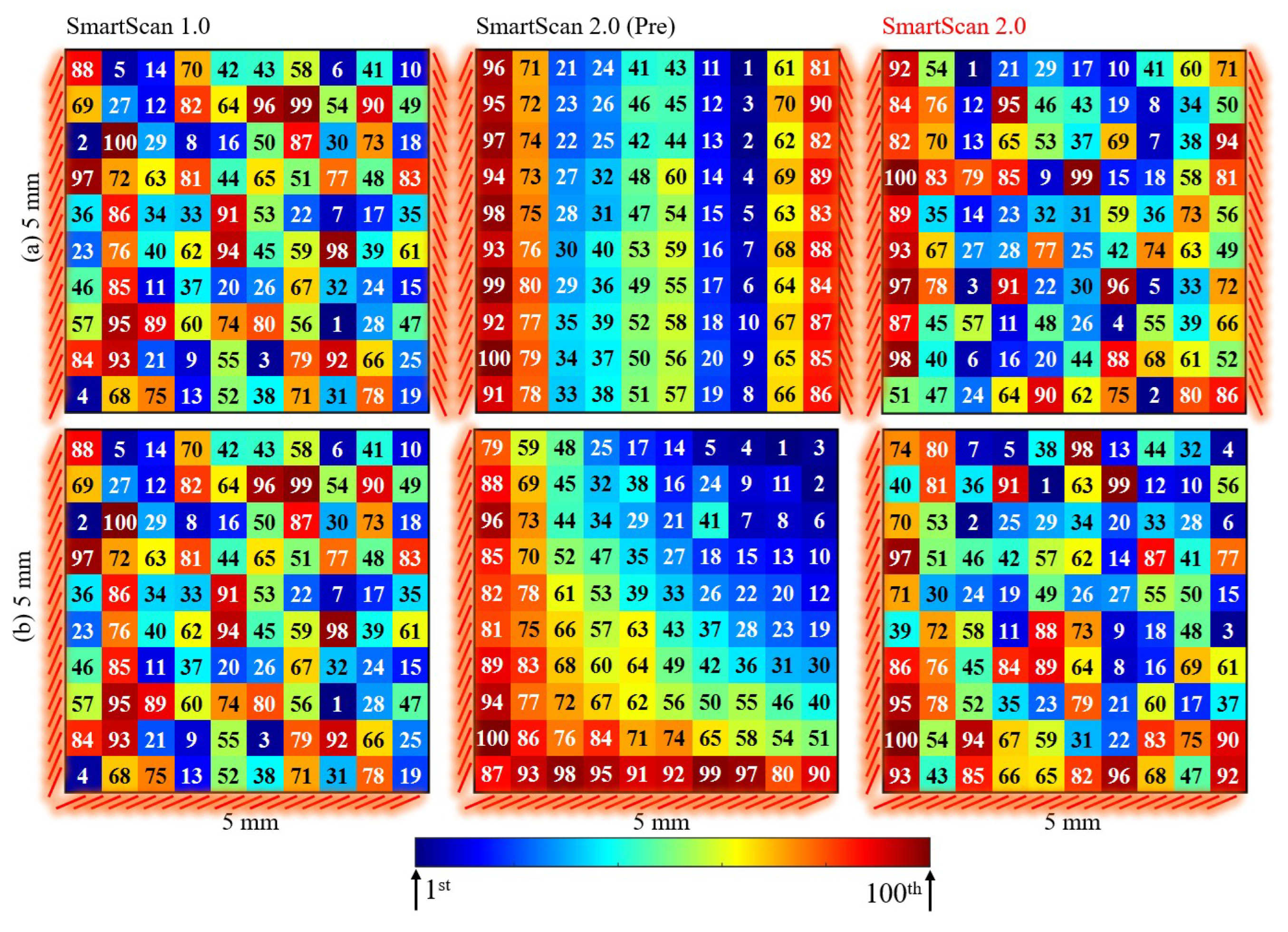
Figure 9.
Comparison of SmartScan 1.0, SmartScan 2.0 (Pre), and SmartScan 2.0 with (a) left and right edges fixed and (b) left and bottom edges fixed using the thermal uniformity metric as defined in Equation (17).
Figure 9.
Comparison of SmartScan 1.0, SmartScan 2.0 (Pre), and SmartScan 2.0 with (a) left and right edges fixed and (b) left and bottom edges fixed using the thermal uniformity metric as defined in Equation (17).
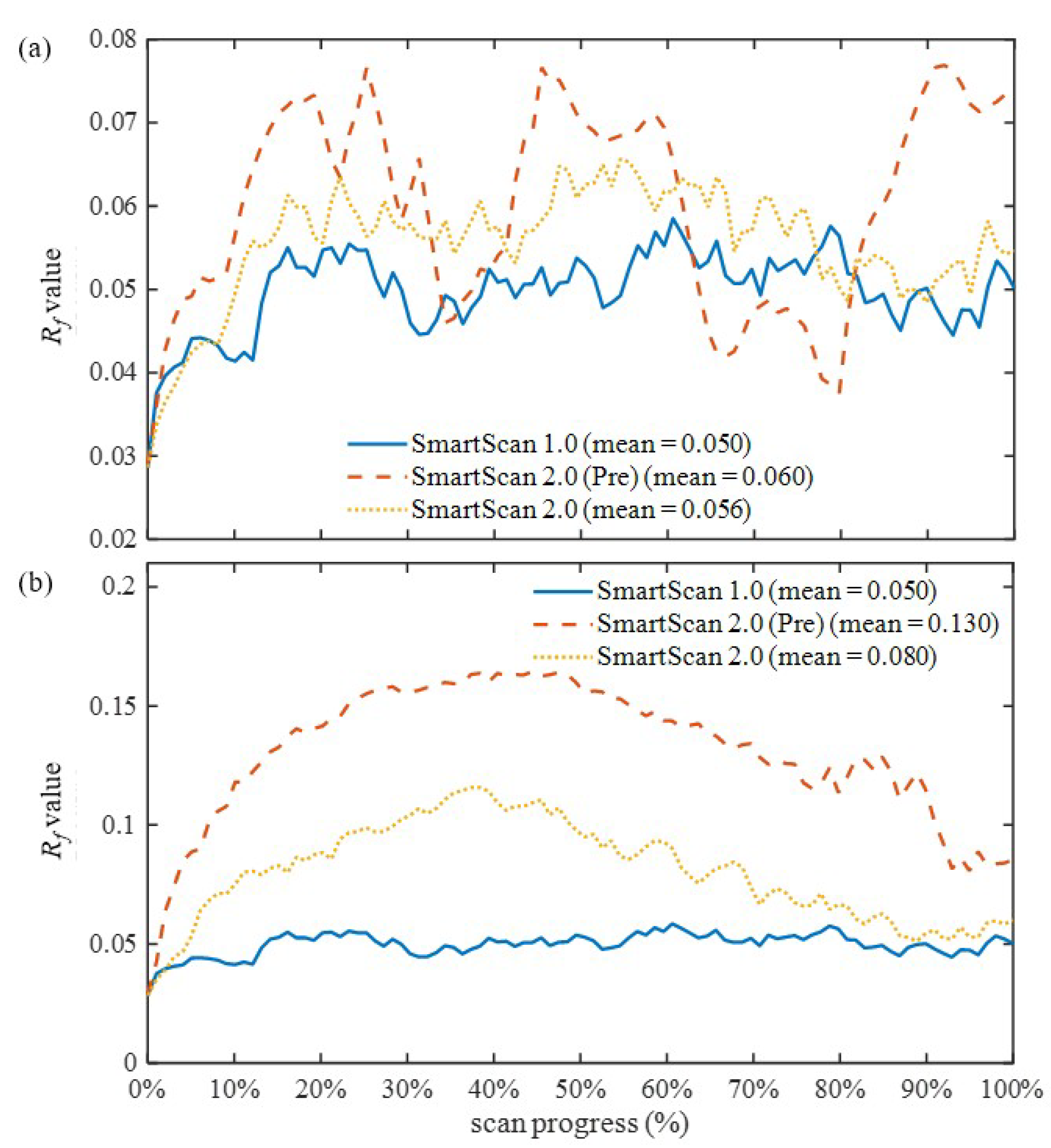
Figure 10.
Comparison of dimensionless temperature fields for SmartScan 1.0, SmartScan 2.0 (Pre) and SmartScan 2.0 at four build completion stages (25%, 50%, 75%, and 100%) using island scanning patterns with (a) left and right edges fixed and (b) left and bottom edges fixed.
Figure 10.
Comparison of dimensionless temperature fields for SmartScan 1.0, SmartScan 2.0 (Pre) and SmartScan 2.0 at four build completion stages (25%, 50%, 75%, and 100%) using island scanning patterns with (a) left and right edges fixed and (b) left and bottom edges fixed.
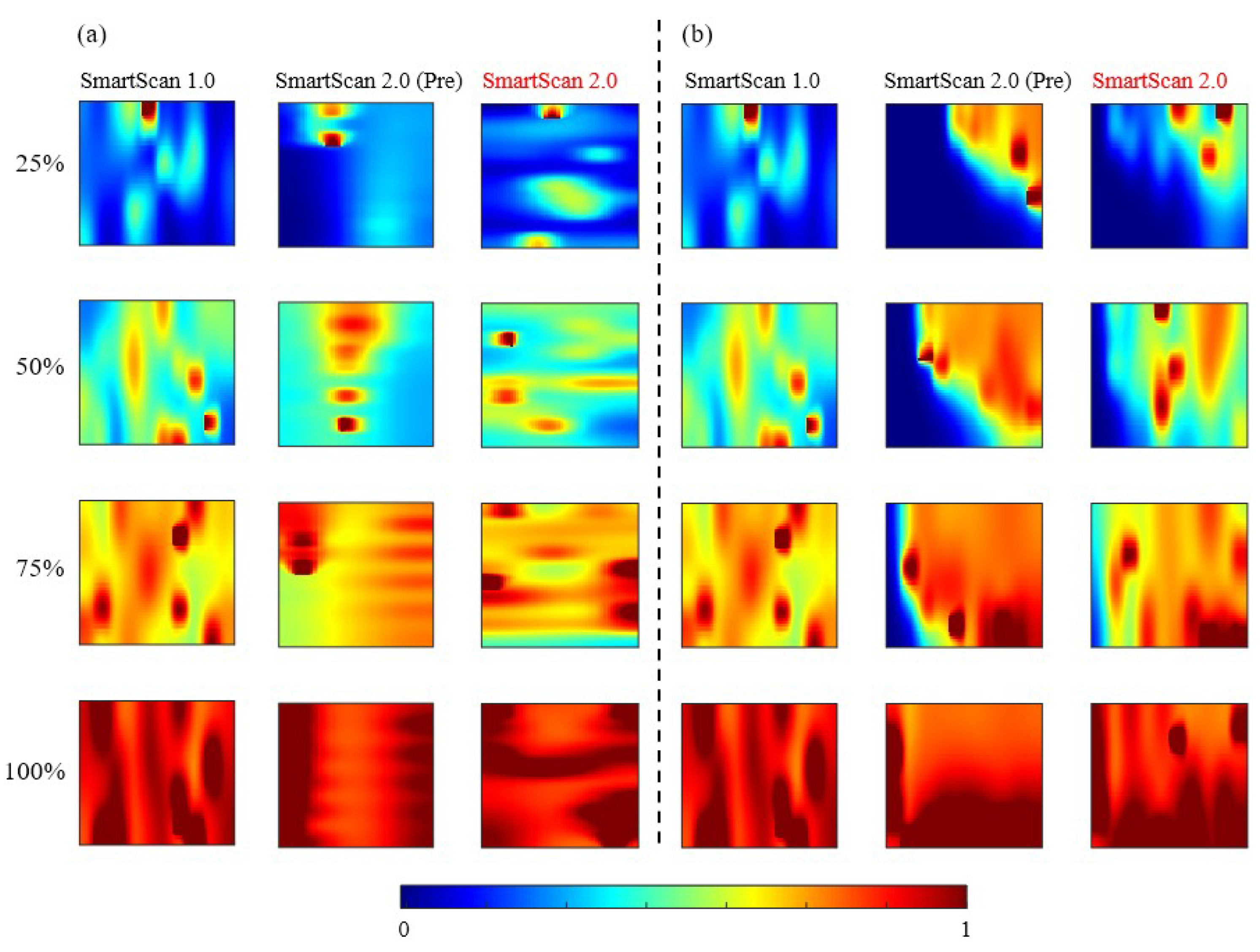
Figure 11.
Comparison of SmartScan 1.0, SmartScan 2.0 (Pre), and SmartScan 2.0 with (a) left and right edges fixed and (b) left and bottom edges fixed using the elastic deformation metric as defined in Equation (13).
Figure 11.
Comparison of SmartScan 1.0, SmartScan 2.0 (Pre), and SmartScan 2.0 with (a) left and right edges fixed and (b) left and bottom edges fixed using the elastic deformation metric as defined in Equation (13).
Figure 12.
Comparison of simulated dimensionless elastic deformation fields for SmartScan 1.0, SmartScan 2.0 (Pre) and SmartScan 2.0 at four build completion stages (25%, 50%, 75%, and 100%) using island scanning patterns with (a) left and right edges fixed and (b) left and bottom edges fixed.
Figure 12.
Comparison of simulated dimensionless elastic deformation fields for SmartScan 1.0, SmartScan 2.0 (Pre) and SmartScan 2.0 at four build completion stages (25%, 50%, 75%, and 100%) using island scanning patterns with (a) left and right edges fixed and (b) left and bottom edges fixed.
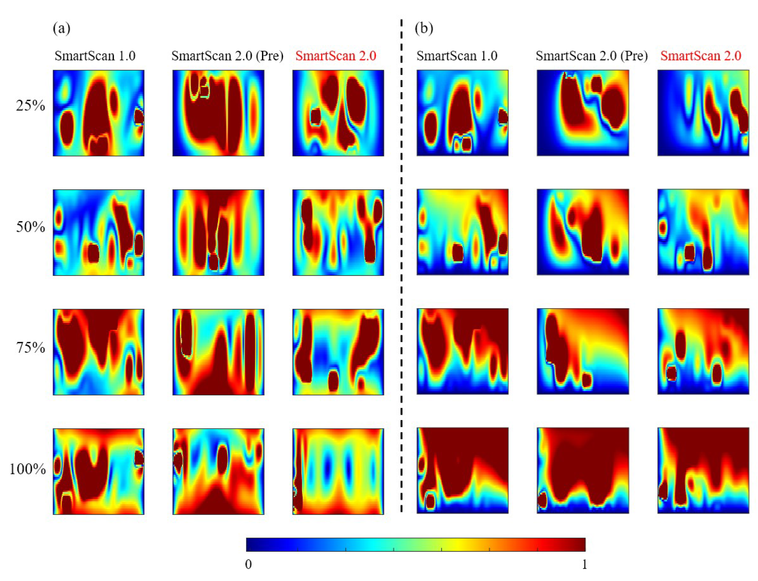
Figure 13.
Measured out-of-plane deformation profiles for plates while clamped, comparing SmartScan 1.0, SmartScan 2.0 (Pre), and SmartScan 2.0 under (a) fully constrained left and right edges and (b) fully constrained left and bottom edges.
Figure 13.
Measured out-of-plane deformation profiles for plates while clamped, comparing SmartScan 1.0, SmartScan 2.0 (Pre), and SmartScan 2.0 under (a) fully constrained left and right edges and (b) fully constrained left and bottom edges.
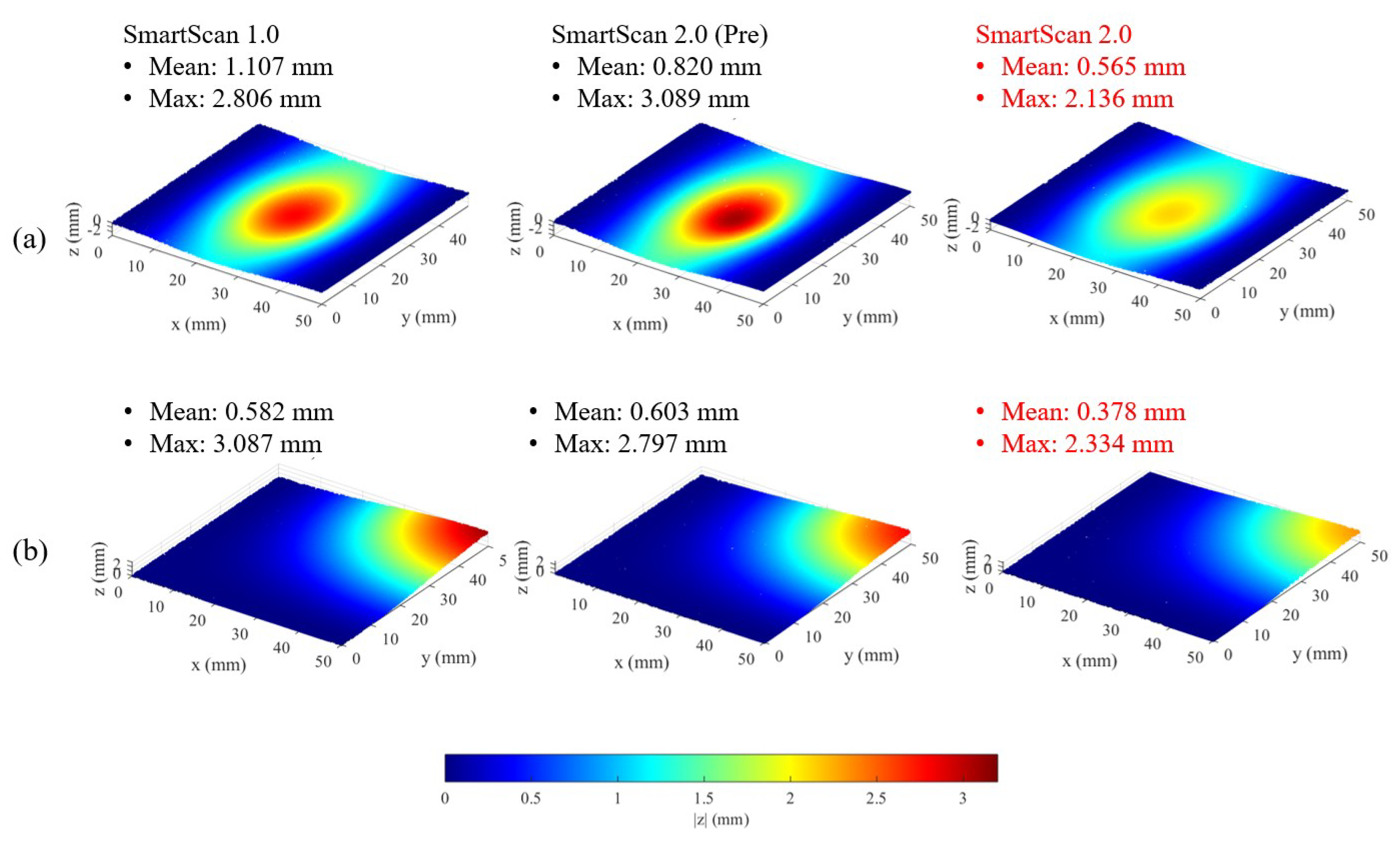
Figure 14.
Measured out-of-plane deformation profiles for plates after unclamping, comparing SmartScan 1.0, SmartScan 2.0 (Pre), and SmartScan 2.0 under (a) fully constrained left and right edges and (b) fully constrained left and bottom edges.
Figure 14.
Measured out-of-plane deformation profiles for plates after unclamping, comparing SmartScan 1.0, SmartScan 2.0 (Pre), and SmartScan 2.0 under (a) fully constrained left and right edges and (b) fully constrained left and bottom edges.
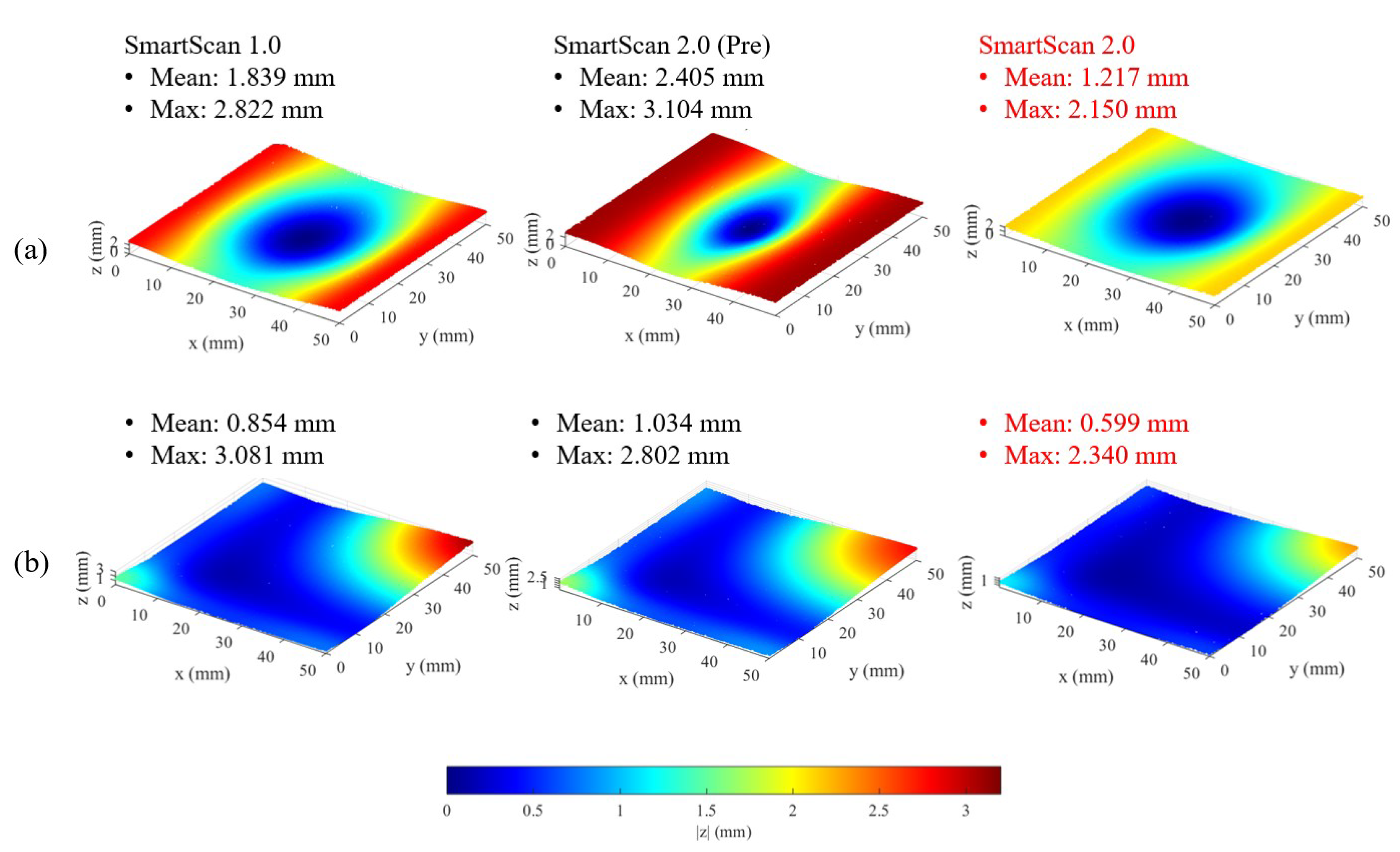
Figure 15.
Cantilever-beam geometry employed in the simulations and experiments for Case Study 2, and the resultant scan sequences for the highlighted Layer 150.
Figure 15.
Cantilever-beam geometry employed in the simulations and experiments for Case Study 2, and the resultant scan sequences for the highlighted Layer 150.
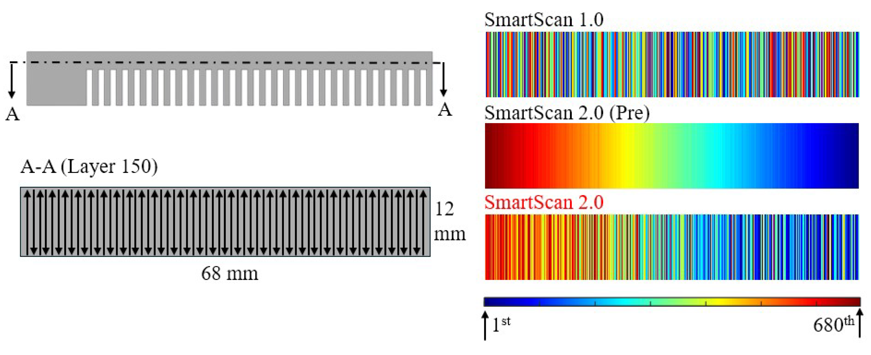
Figure 16.
Printed parts using the SmartScan 1.0, SmartScan 2.0 (Pre) and SmartScan 2.0 sequences, and the analysis of the deformation of their top surfaces.
Figure 16.
Printed parts using the SmartScan 1.0, SmartScan 2.0 (Pre) and SmartScan 2.0 sequences, and the analysis of the deformation of their top surfaces.
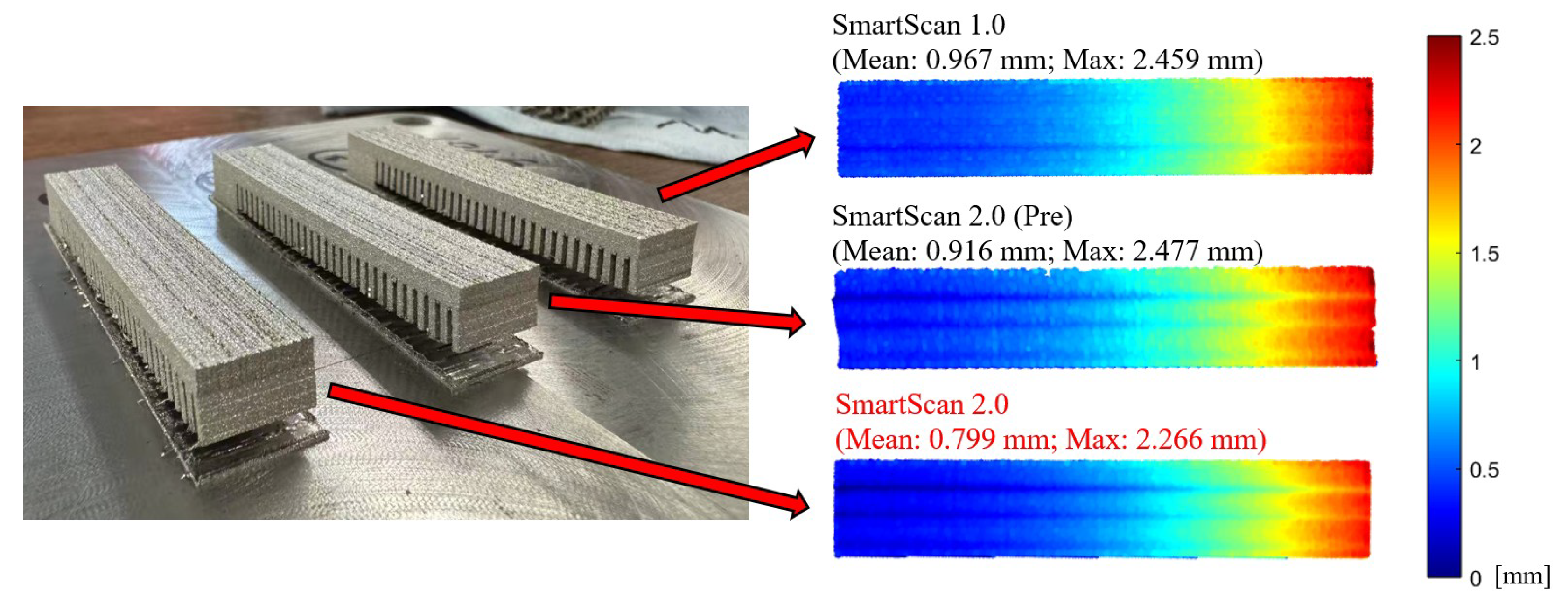
Figure 17.
X- and Y-direction residual stresses measured on the printed part using the SmartScan 1.0, SmartScan 2.0 (Pre) and SmartScan 2.0 sequences
Figure 17.
X- and Y-direction residual stresses measured on the printed part using the SmartScan 1.0, SmartScan 2.0 (Pre) and SmartScan 2.0 sequences
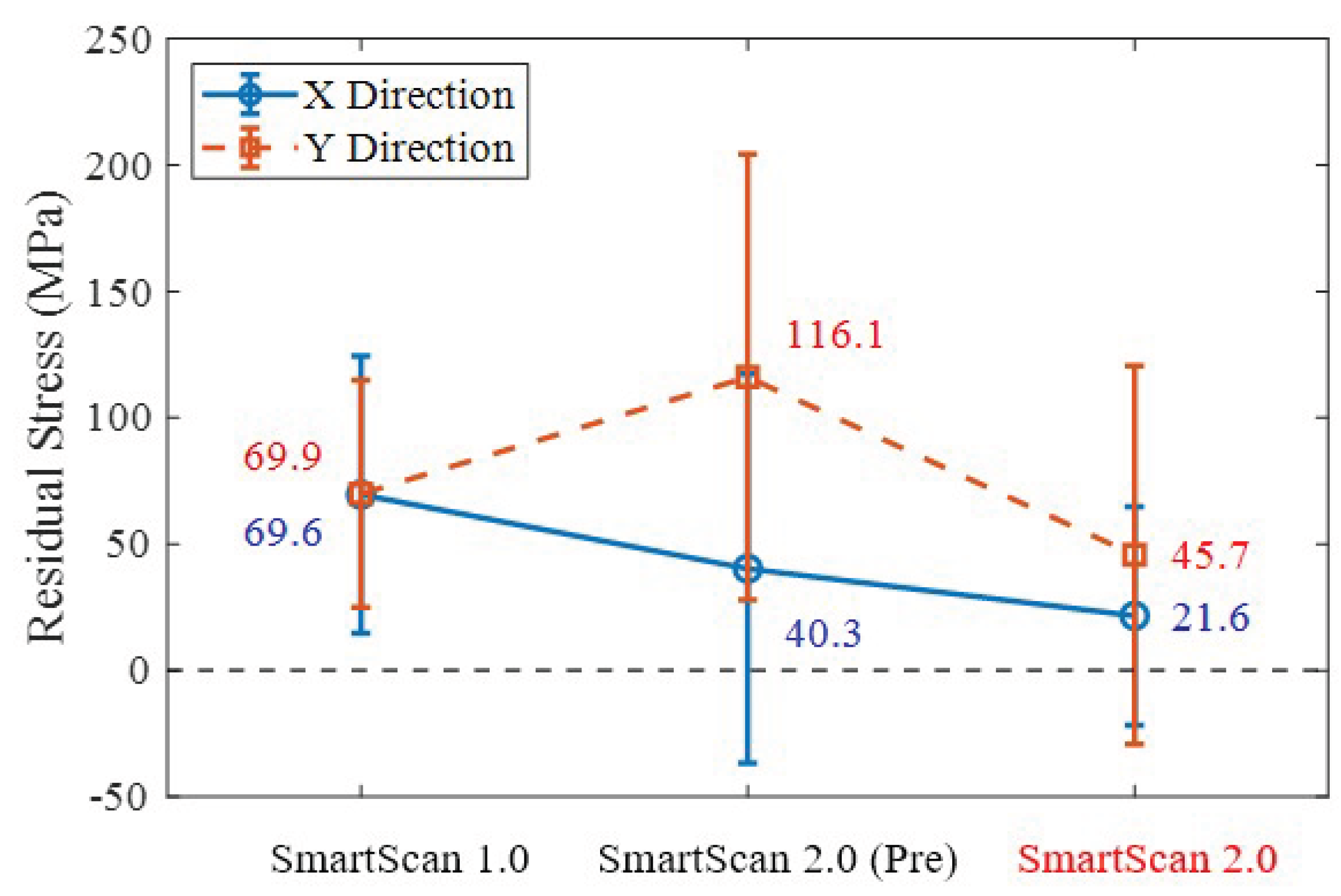

Table 1.
Thermal and elastic parameters for SS316L, with temperature-dependent values evaluated at , which is a representative in-build LPBF temperature that balances property variation across the build [1].
Table 1.
Thermal and elastic parameters for SS316L, with temperature-dependent values evaluated at , which is a representative in-build LPBF temperature that balances property variation across the build [1].
| Parameter (Units) | Value |
|---|---|
| Laser power, P (W) | 290 |
| Laser spot diameter () | 78 |
| Absorptance, | 0.37 |
| Mark/scan speed (mm/s) | 1200 |
| Jump speed (mm/s) | 6000 |
| Hatch spacing in Case Study 1 () | 200 |
| Hatch spacing in Case Study 2 () | 100 |
| Layer thickness () | 50 |
| Dimensionless Model Configuration (units) | Value |
| Nondimensional spatial step, | |
| Nondimensional time step, | |
| Characteristic length, ℓ in Case Study 1 (mm) | 50 |
| Characteristic length, ℓ in Case Study 2 (mm) | 68 |
| Characteristic temperature difference, (K) | 1658 |
| Characteristic volumetric heat generation, Q | |
| Thermal properties (evaluated at 550 K) | |
| Thermal conductivity, | 23.5 |
| Thermal diffusivity, | |
| Specific heat, | 540 |
| Density, | 7900 |
| Melting temperature, (K) | 1658 |
| Convection coefficient, h | 25 |
| Ambient temperature, (K) | 293 |
| Heat sink temperature, (K) | 293 |
| Elastic model parameters (evaluated at 550 K) | |
| Young’s modulus, E (GPa) | 160 |
| Poisson’s ratio, | 0.30 |
| Coefficient of thermal expansion, | |
Table 2.
Computation time in seconds for the two boundary conditions in Case Study 1.
| Boundary Condition #1: left and right edges fully constrained (s) | Boundary Condition #2: left and bottom edges fully constrained (s) | |
| SmartScan 1.0 | 14.1 | 12.8 |
| SmartScan 2.0 (Pre) | 11.5 | 10.3 |
| SmartScan 2.0 | 12.9 | 13.1 |
Table 3.
Printing time for the evaluated scan sequences.
| Vector Pattern | Print Time [min] |
|---|---|
| SmartScan 1.0 | 34.7 |
| SmartScan 2.0 (Pre) | 28.7 |
| SmartScan 2.0 | 32.0 |
Disclaimer/Publisher’s Note: The statements, opinions and data contained in all publications are solely those of the individual author(s) and contributor(s) and not of MDPI and/or the editor(s). MDPI and/or the editor(s) disclaim responsibility for any injury to people or property resulting from any ideas, methods, instructions or products referred to in the content. |
© 2025 by the authors. Licensee MDPI, Basel, Switzerland. This article is an open access article distributed under the terms and conditions of the Creative Commons Attribution (CC BY) license (http://creativecommons.org/licenses/by/4.0/).
Copyright: This open access article is published under a Creative Commons CC BY 4.0 license, which permit the free download, distribution, and reuse, provided that the author and preprint are cited in any reuse.


