
Submitted:
11 November 2025
Posted:
14 November 2025
You are already at the latest version
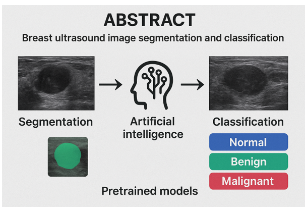
Abstract
Breast ultrasound image segmentation and classification are the two crucial steps for early diagnosis of cancer. In this work we developed a breast cancer segmentation and multiclass classification artificial intelligence tools based on pretrained models. The proposed workflow includes both the development of a segmentation model architecture and second the development of a series of classification models to classify the ultrasound greyscale images into normal, benign or malignant. The training and testing of the pretrained models were performed using the Breast Ultrasound Images (BUSI dataset). For the image segmentation task, the models were trained on the images while using masks as target variable. In the multiclass classification, each image was provided with accurate label “benign”, “normal” or “malignant” and used to train a multiclass classifier. Optuna was used for hyperparameter optimization and for the testing of various pretrained models to determine the best encoder (ResNet18, EfficientNet-B0 & MobileNetV2)-decoder (U-Net, U-Net++, DeepLabV3) image segmentation architecture. For multiclass classification, five different pretrained models (ResNet18, DenseNet121, InceptionV3, MobielNetV3, GoogleNet) were optimized and tested for their ability to classify breast cancer images. The developed Image segmentation models performed well in terms of delineating the lesion in the breast ultrasound images. DeepLabV3 outperformed other segmentation architectures with consistent performance across train, validation and test images with Dice Coefficients of 0.87, 0.80 and 0.83 respectively. ResNet18:DeepLabV3 achieved an Intersection over Union score of 0.78 during training. ResNet18: U-net++ achieved best Dice coefficient (0.83) and IoU (0.71) and AUC score of 0.91 on the test (unseen) dataset when compared to other models. For classification of breast cancer images, ResNet18 achieved an F1 score of 0.95 and an accuracy of 0.90 on the train dataset, while InceptionV3 outperformed other models on the test dataset with an F1 score of 0.75 and accuracy of 0.83. We demonstrate a comprehensive approach to automate the image segmentation and multiclass classification of breast cancer ultrasound images into benign, malignant or normal using transfer learning models on an imbalanced ultrasound image dataset.
Keywords:
breast cancer
; ultrasound image analysis
; artificial intelligence
; pretrained models
; transfer learning
; U-net
; U-net++
; DeepLabV3
; multiclass classification
; Optuna optimization
1. Introduction
The goal of this study is to develop automated breast cancer detection tools that can both segment and classify breast ultrasound images using transfer learning with pretrained model weights. Breast cancer is the leading cause of cancer-related deaths among women. A 2024 study shown that around 1 in 8 women (13%) will be detected with breast cancer, and 1 in 43 (2.3%) will die from the breast cancer [1]. This type of cancer develops in the breast tissue and can form tumors that are detectable using various imaging techniques. Ultrasound imaging is extensively used to evaluate breast tissue for potential malignant masses due to its non-invasive nature [3]. Unlike X-ray-based imaging procedures, ultrasound techniques do not use ionizing radiations, making them safer for repeated use and more cost-effective compared to other imaging modalities [2].
Breast ultrasound images can be categorized into three types, normal images, images with benign tumors and images with malignant tumors. An important step in breast cancer diagnosis is classification of the ultrasound images into benign, malignant, or normal. In traditional assessment of breast ultrasound images, it is difficult to distinguish subtle indicators of malignancy from benign features, specifically with lesions that do not show clear boundaries on the ultrasound scans [10]. Thus, leading to false negatives where radiologists consider a malignant tumor as benign and potentially missing out the on early detection of the malignant tumor. Similarly, there is risk for false positives, where benign or normal tissue is mistakenly evaluated as malignant. Medical image segmentation is a challenging task, and field of image processing is crucial for radiologists in delineating lesions to obtain measurements such as tumor size, shape and volume.
Image segmentation techniques can enable better monitoring of tumor growth and treatment response by allowing radiologists to concentrate on the region of interest without being distracted by the surrounding tissues, [5]. However, process of manual image segmentation and classification can also result in misdiagnosis. Further those processes are time-consuming and prone to human error due to variations in interpretation style and experience among radiologists [4]. Thus, developing automated tools is critical to enhance the reliability and efficiency of the breast cancer diagnosis process, particularly image segmentation and classification of tumors as normal, benign or malignant. By training deep learning models on extensive and diverse image datasets, they can learn to detect subtle edges and intricate patterns that may not be visible to human eye.
Recent developments in Convolutional Neural Networks (CNNs) have provided outstanding solutions for medical image analysis [6-9]. Fully convolutional networks (FCNs), U-Net are cutting-edge deep learning models designed to handle complex input data. These models use deep neural nets to process data by hierarchically extracting features via hidden layers and iteratively training the networks [12]. Soulami et al., developed U-net model with mammogram datasets to delineate the lesions and classify outcomes of the diagnosis as benign or cancerous. They reported an intersection over union of 90.50% and an AUC of 99% [24]. Additionally, a Fuzy logic Network in combination with eight CNN-based pretrained models was trained to perform semantic segmentation on the BUSI dataset [38].
In another study, a hybrid CNN- transformer network was developed for breast cancer ultrasound image segmentation by using transformer encoder blocks in the encoder part of the CNN-transformer net to learn the global contextual information then combined with a CNNs to extract features. Whereas in the decoder part they used spatial-wise cross attention module to reduce the semantic discrepancy with the encoder [25]. Guo et al developed U-shaped convolutional neural networks (U-Net) for semantic segmentation of the breast cancer ultrasound images. They reported the average Dice coefficient and average intersection of Union (IoU) coefficient of 90.5% and 82.7% respectively [27]. In 2024, Nastase et al developed and tested two segmentation architectures for delineating the lesion in the breast cancer ultrasound images. They reported that DeepLabV3 outperformed the U-net in terms of binary classification with average dice score 0.93 and 0.9 on malignant and benign classes [28]. Yap et al [45] developed LeNet, Unet and FCN-AlexNet and compared against four traditional methods that relied on manually designed features and rules. Among the developed models, FCN-AlexNet demonstrated the highest performance with F1 score of 0.92.
In another study comparison of the performance of FCN, U-net, DenseNet121 and PSPNet models in terms of IoU, accuracy, precision, F1 score, they reported that their model achieved a 95% prediction accuracy in terms of image segmentation of the histology dataset of breast cancer [29]. Similarly, transfer learning techniques were used to perform binary and multiclass classification of the breast cancer ultrasound images. For example, [30] leveraged transfer learning techniques using pretrained models. They developed ResNet50, ResNeXt50 and VGG16 models to classify breast cancer ultrasound images into benign, malignant and normal images. They reported ResNetXt50 had an accuracy of 85.83%, ResNet50 accuracy of 85.4% and VGG16 has lowest accuracy of 81.11% [30]. In another study a GoogleNet and residual blocks inspired model with learnable activation functions was developed to conduct image classification [31]. They reported their models showed an accuracy of 93% on breast cancer ultrasound images and the F1 score of their model variants range between 0.88 and 0.93 with Loss value ranging between 0.21 and 0.3 [31].
Various approaches have been proposed in the literature to address the problem of breast cancer segmentation and classification using the BUSI dataset, but there are fewer comprehensive reports that include both development of segmentation and classification models based on transfer learning for breast cancer image segmentation and multiclass classification. UNETR network [33] was optimized and trained to conduct image segmentation and classification on the lung cancer image dataset by Said et al in 2023. They reported that their first task of image segmentation achieved an accuracy of 97.83% and in the second task of classification they achieved a 98.77% accuracy [39].
This work aims to evaluate and compare the performance of U-Net, U-Net++ and DeepLabV3 segmentation models by integrating encoder-decoder architecture with a shared feature extraction backbone. For the encoder part of the segmentation model, the pretrained models: ResNet18, EfficientNet-B0 and MobileNetV2, were tested. The second part of this work is to develop a multiclass classification model for classifying BUSI into malignant, benign or normal. To this end, we have developed and optimized pretrained models including ResNet18, InceptionV3, DenseNet121, MobileNetV3 and GoogleNet. The main contribution of this work includes proposal of an automatic breast cancer segmentation and classification systems. Testing various pretrained models as encoder in the encoder: decoder architectures of the U-Net, U-Net++ and DeepLabV3 segmentation models. Optimization of the hyperparameters of the segmentation models and classification models using Optuna and validation of the proposed segmentation and classification models was conducted on the BUSI dataset.
2. Materials and Methods
2.1. Dataset
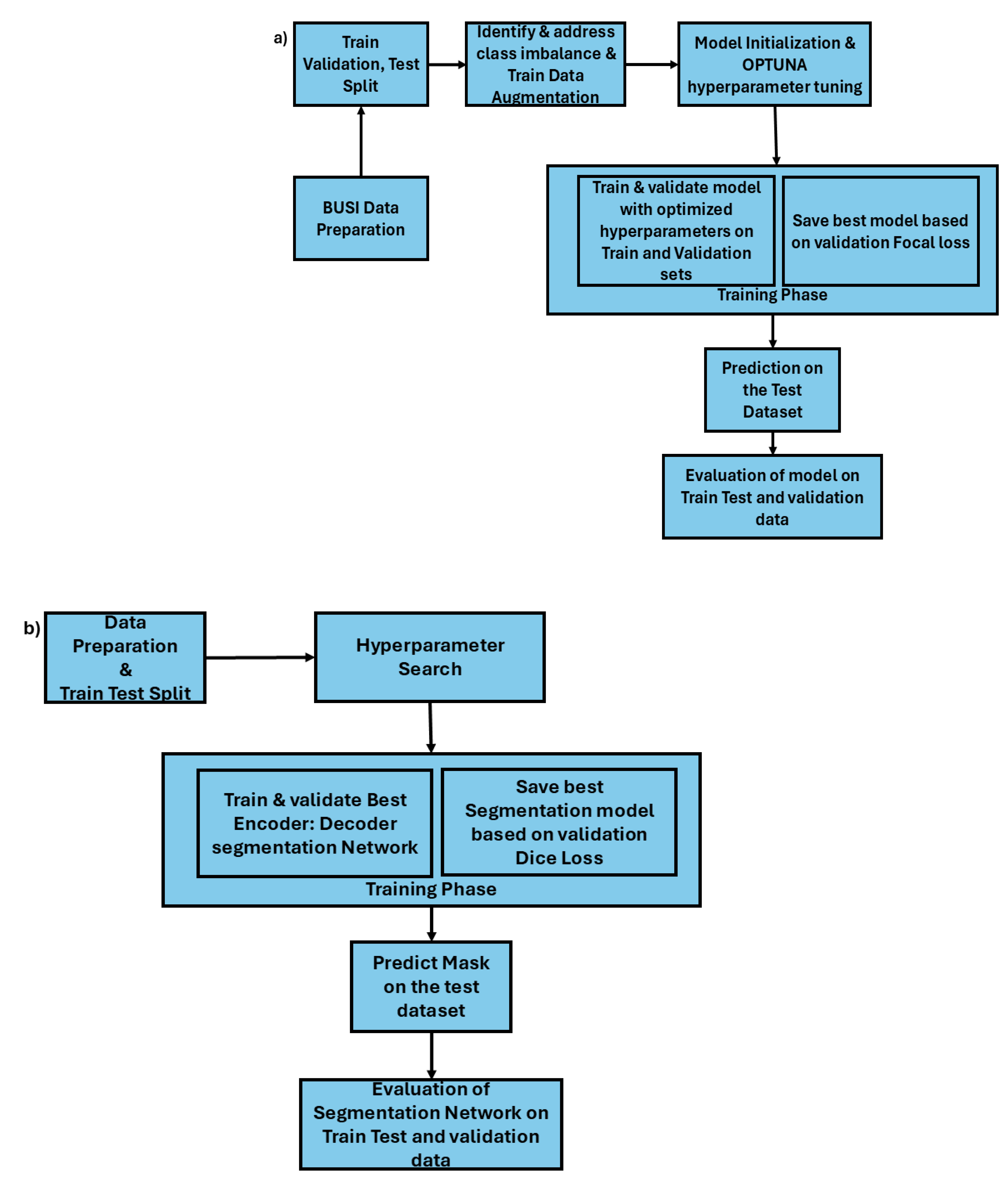
BUSI dataset [34] was utilized for both segmentation and classification tasks in this study. Image segmentation and classification of the BUSI dataset remained a challenging task due to its poor image quality [26]. This dataset contains 780 images, categorized into three classes normal (132), benign (436), and malignant (210). Figure 2b) depicts the workflow of the breast cancer classifier development methodology. The first step of the development process is data preparation, in this step the dataset was divided into training, validation and test sets using an 80:10:10 split, and proportional representation of each class across the sets was ensured. In this study train and validation datasets were used in the training phase of the models and the test dataset was only used in the inference phase to evaluate the model performance and generalization on the unseen data. Table 2 shows the distribution of the images specific to each label. From the Table 2 it is evident that the dataset is an imbalanced dataset containing a greater number of instances with the “benign” label compared to “normal” or “malignant” samples.

Table 1.
Data distribution of image-mask pairs for binary segmentation task.
| Train Dataset | Validation dataset | Test dataset | |||
| Images | Masks | Images | Masks | Images | Masks |
| 624 | 624 | 77 | 77 | 77 | 77 |
Table 2.
Dataset distribution of the images for multiclass classification task.
| Ultrasound Breast images | Train dataset | Validation dataset | Test dataset |
| Benign | 350 | 43 | 43 |
| Malignant | 168 | 21 | 21 |
| Normal | 106 | 13 | 13 |
| Total | 624 | 77 | 77 |
Figure 1.
Sample image and mask pair data for image segmentation task.
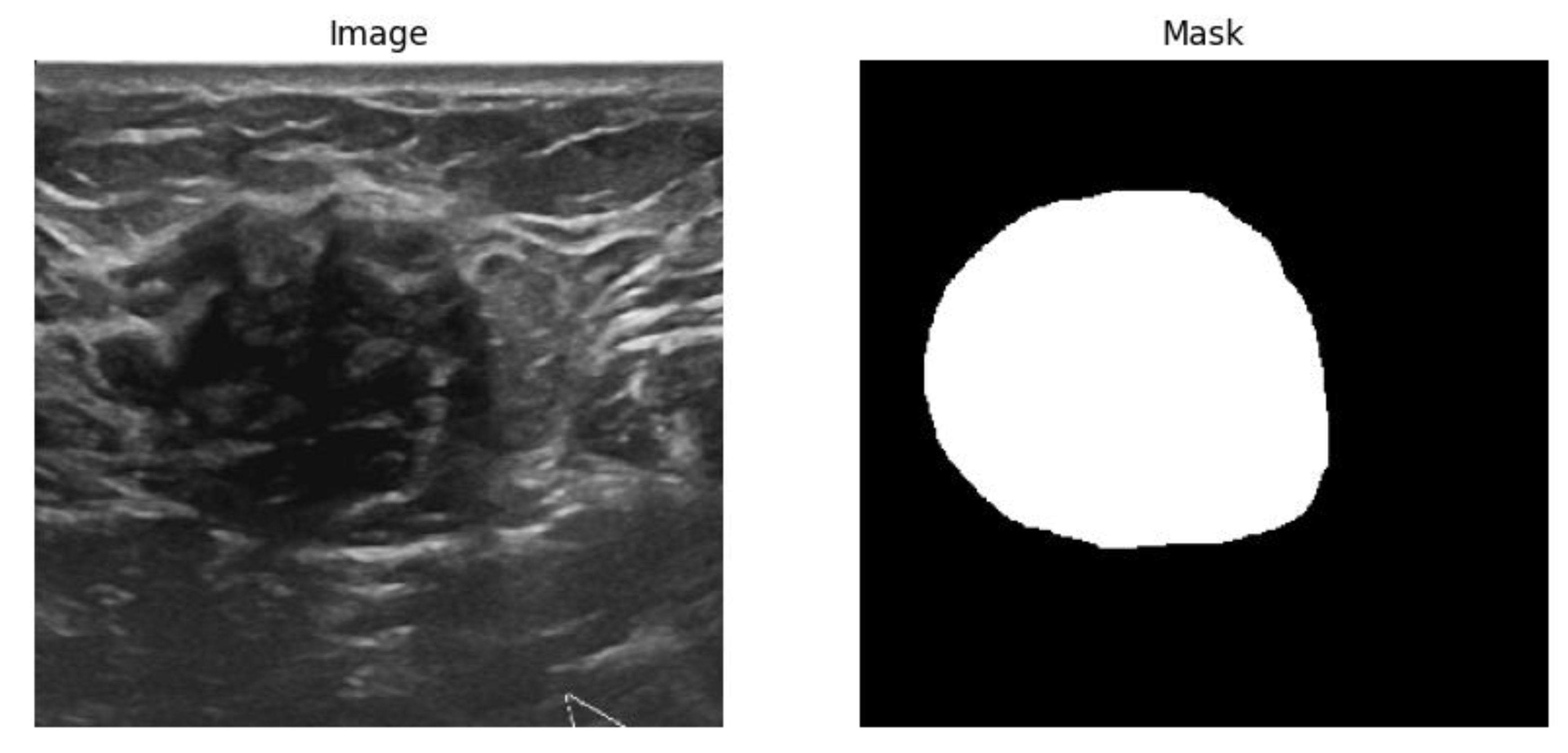
Figure 2.
a) Breast Cancer segmentation using encoder: decoder architecture b) Multi class Classification of breast cancer images.
Figure 2.
a) Breast Cancer segmentation using encoder: decoder architecture b) Multi class Classification of breast cancer images.
2.2. Segmentation Models
The segmentation models U-Net, U-Net++ and DeepLabV3 were trained and tested to predict the masks of the BUSI to segment the lesions of the images.
2.2.1. U-Net
U-Net is a CNN model architecture originally designed for working well on the smaller medical imaging datasets predominant in field of biomedical engineering.[11]. Based on the fully convolutional network (FCN), the U-Net architecture is expanded to include other encoder: decoder paths that are designed for contracting and expanding the features of the input images. The encoder captures the context by reducing the spatial dimensions while increasing the feature depth through a series of convolutional (1) and pooling (2) operations, mathematically represented by equations (1) & (2) respectively.
Where is rectified linear Unit (ReLU) activation function, X is the input, W is the learnable filter with bias b to generate feature map Y, and R is the receptive field over which the max pooling operation is applied. The max pooling operations are applied at each encoder level gradually capturing the high-level features.
The decoder architecture reconstructs the segmentation map by up sampling the feature maps to match the original input resolution using transposed convolutions. Further the U-Net architecture makes use of skip connections between encoder and decoder layers. Feature map are concatenated with corresponding feature map of the decoder , improving spatial accuracy in segmentation as shown in the equation (3)
Where represents concatenation along the feature dimension, and f is subsequent convolutional layers applied at each decoder stage. In the final layer, 1×1 segmentation is applied to map the output to the desired number of classes producing segmentation map by classifying each pixel as shown in the equation (4).
Where is a filter that maps to channels, with each channel representing one class probability, normalized by SoftMax function. An in-depth mathematical explanation of U-net architecture can be obtained in recently published research work [13].
2.2.2. U-Net++
The U-Net++ model is built upon U-Net architecture by introducing two structural improvements: nested skip pathways and deep supervision [14], [15]. Unlike U-Net, encoder: decoder architectures of the U-Net++ are connected using nested, dense convolutional blocks [46]. The feature map connecting encoder level to decoder level . The mathematical representation of the convolutional blocks is given by equation 5
Where is the feature map at encoder level and decoder level after convolutional layers, ⊕ is the concatenation across the feature dimensions and represents convolutional layers applied on concatenated feature map. Deep supervision [15] enables the model to operate in “accurate” mode or “fast” mode. In the accurate mode the outputs from all segmentation branches are averaged, whereas in the “fast” mode, final segmentation map is selected from only one of the segmentation branches. The selection between the two modes results in model pruning and speed gain.
2.2.3. DeepLabV3
DeepLabV3 was proposed by Google Brain team [36]. It uses the concept of atrous spatial pyramid pooling convolutions (ASPP) [35] to control the receptive fields thereby capturing wider context of the images without reducing the image resolution. Deep convolutional neural networks (DCNN’s) suffer from reduced spatial resolution due the pooling and striding techniques used in DCNN’s. DeepLabV3 addresses this issue by using cascading atrous convolutions with varying rates to capture multiscale contextual information. ASPP convolutions in DeepLabV3 contains image-level features that provide global context via global pooling, followed by a 1×1 convolution, batch normalization and up sampling. A detailed mathematical explanation and research methodology of DeepLabV3 is explained in detail in [36].
2.3. Classification Models
2.3.1. ResNet18
He et al., in 2015, introduced deep residual networks (ResNet) for image recognition [16]. ResNet18 consists of 18 convolutional layers with an input layer with image size of 3×244×244. ResNet18 contains four blocks of neural networks, each block containing two basic locks of two convolutional layers with last layer being a fully connected layer thus total 18 layers. This network solves the vanishing gradient problem through skip connections that adds the input of the block to its output. ResNet learns identity mapping using skip connections and is suitable for various image segmentation and classification tasks.
2.3.2. GoogleNet
GoogleNet also known as InceptionV1 is a CNN architecture proposed by [17]. Inception architecture is based on the Network in Network structure proposed by [18]. The inception architecture increases the network width by using multi-input layers and multiple convolution kernels of different sizes to capture wide range and details from input images. GoogleNet has 22 layers of network but only 1/36th of the parameters of the VGG [19].
2.3.3. InceptionV3
InceptionV3, developed by the Google Brain team, achieved a top-5 error rate of 3.46% on the ImageNet dataset. In 2016, Google released the latest version of the inception model containing 48 layers and introduces factorized convolutions, which replace 5×5 kernels with two 3×3 kernels to maintain the performance while reducing computational load. The input layer of the inceptionV3 receives 3×299×299. InceptionV3 consists of three components: the convolutional block, multiple inception modules and final classifier [21]. The initial convolutional block contains alternative convolutional and max pooling layers to extract features from the input image. The inception modules perform multiscale convolutions in parallel using kernels of different sizes (1×1, 3×3 and 5×5) followed by concatenation to capture diverse features [20]. The final classifier includes fully connected layers with a SoftMax layer at the end to output class probabilities for the target classes.
2.3.4. MobileNetV3
MobileNetV3 [22] is designed for efficient image classification, specifically to run on the mobile and edge devices. This model was released in 2019 by the Google Brain team, the input layer of the MobileNetV3 accepts images of size 3×244×244. It consists of convolutional block, multiple MobileNetV3 modules and a final classifier. The primary features are extracted using the initial convolutional block with batch normalization and a ReLU activation function. The core of the architecture includes squeeze-and-excitation (SE) modules embedded in the bottleneck and inverted residual blocks with depth wise separable convolutions.
2.3.5. DenseNett121
DenseNet121 introduces dense connectivity between layers, where each layer is directly connected to every subsequent layer within a dense block, creating a densely connected network structure. Unlike CNNs where the information passes subsequently from one layer to the next, DenseNet121 contains direct pathways from each layer to all subsequent layers through feature map concatenation [23]. It contains three main components: a convolutional block multiple dense blocks connected by transition layers and final classifier. In the dense block of L layers, each layer l receives the feature maps of all preceding layers [0,..,l-1] as input, leading to connections. Each layer adds its own feature maps to the network’s collective knowledge, where is the growth rate hyperparameter. This means the Lth layer has input features, where is the initial number of features. These dense connections allow feature reuse and strengthens gradient flow and solves the vanishing gradient problem by providing multiple paths for information propagation.
2.4. Evaluation Metrics
The performance of the proposed models was tested using several standard evaluation metrics that are widely used in image segmentation and classification tasks. These metrics provide comprehensive account on the model’s effectiveness in terms of accuracy and precision and reliability.
2.4.1. Intersection over Union (IoU)
Intersection over Union is also known as Jaccard Index, is used for evaluating the segmentation quality. It measures the overlap between the predicted segmentation mask and ground truth mask. IoU penalizes both over-segmentation and under segmentation, providing balanced assessment of the segmentation accuracy. The IoU is mathematically expressed as below
Where A represents the predicted segmentation mask and B is the ground truth mask.
2.4.2. Confusion Matrix
Confusion matrix provides a detailed breakdown of the model’s performance across different classes. It provides a tabular summary of the predicted class labels with the true class labels, offering a detailed insights into the model’s performance across all classes. For a classification task with n class labels, the confusion matrix is an table where rows represent the actual classes and columns represents the predicted classes. The table contains True Positives (TP); Cases correctly predicted as positive cases, False Positives (FP); Classes where the model incorrectly predicted the positive classes. False Negatives (FN); Classes where the model incorrectly predicted the negative class. True Negatives (TN); Cases correctly predicted as the negative class.
2.4.3. Pixel Accuracy
Pixel accuracy represents the proportion of correctly classified pixels across all classes. It is calculated as shown in equation 7.
2.4.4. AUC
The area under the receiver operating characteristic (ROC) curve, commonly known as AUC, evaluates the model’s ability to distinguish between classes across various classification thresholds. The AUC score ranges from 0 to 1 where, AUC =1 represents perfect classification, AUC = 0.5 indicates random classification and AUC<0.5 suggests worse than random classification.
2.4.5. Dice and Focal Loss
Dice Loss (DL) is a loss function that measures the overlap between predicted segmentation masks and the ground truth masks. DL is derived from Dice Similarity Coefficient (DSC) which is used to find the similarity between two sets. DL is particularly useful when dealing with imbalanced datasets because it emphasizes regions of interest to improve the accuracy of the segmentation models by prioritizing overlap. DSC is defined as shown in equation 8.
Where is the set of predicted pixels and is the set of actual pixels. || is the number of pixels common for both X and Y. DSC can also be mathematically represented in terms of individual pixels and ground truth pixels as shown in the equation 9
(9)
Where is the predicted probability for the pixel, is the ground truth label for the and N is the total number of pixels. The Dice loss is then calculated using the Dice coefficient as shown in the equation 10.
Similarly for the classification task, focal loss was used to optimize the models during the training process. Focal loss was introduced in 2017 and is designed to address class imbalance by focusing on the hard to classify instances [37]. It is a modification of the cross-entropy loss by adding a modulating term (, reducing the loss contribution of well-classified instances allowing the model to focus on the hard cases. For correctly classified samples, is close to 1 and (1- ) approaches 0 reducing the contribution of such samples to the loss. When = 0, the term ( is equal to 1 which is simplifies to standard cross-entropy. For a three-class classification task the focal loss that is minimized during the training process is mathematically defined as shown in equation 11.
Where c is the classes 1,2 and 3. is the class specific weight factor for class c. The value of c lies between 0 and 1 giving more weight to underrepresented classes in the imbalanced dataset. is a variable which ensures that FL is focused on the true class during the training. =1 if class c is true class for the sample and 0 otherwise. To evaluate the performance of the models on the train, test and validation datasets, Precision, Recall and F1 score and their macro average were calculated from the confusion matrix results. Macro averaging is a technique used to address dataset contain imbalanced classes, macro averaging treats each class equally and does not weight larger classes more than the smaller classes. is the penalty term that penalizes incorrect predictions based on the model’s confidence level. While is model’s predicted probability for class c for a given sample. For the true class is high; the further is from 1, the higher the penalty imposed by the loss function.
2.4.6. Precision & Recall
Precision measures the total number of actual positives out of predicted positives. It is a ratio of true positives to the total number of positive predictions. Precision is mathematically defined by equation 12. Recall also known as sensitivity, measures the ability of the model to correctly identify all relative instances. It is mathematically represented by equation 13.
2.4.7. F1 Score
F1 score is a harmonic mean of precision and recall. It is commonly used on the imbalanced datasets since, the harmonic mean emphasizes the lower value between precision and recall. Thus, F1 score will be lower if either precision or recall is low, reflecting the performance of the model more accurately in cases where there is an imbalance between the two metrics. F1 score is mathematically represented by the equation 14.
3. Methodology
In this study, image segmentation architectures were trained on the images with the corresponding segmentation masks as ground truth labels. In the classification task, the models were trained solely on the images, with the target labels being normal, benign and malignant. Since deep learning models require large amount of data to attain ideal performance and BUSI dataset is relatively small, data augmentation techniques were applied to increase the effective size of training set. The data augmentations implemented including random horizontal and vertical flips, random rotations and color jitter. The images were resized according to the requirements of the specific models used for classification. For example, during augmentation, images were resized to 224×224 for ResNet18 and to 299×299 for InceptionV3 to match the input dimensions expected by each model during breast cancer classification task. Both segmentation and multiclass classification tasks were performed using the PyTorch deep learning framework on an NVIDIA RTX 4060 Ti 16 GB external GPU housed in a Node Titan enclosure, connected via Thunderbolt USB-C cable to a Dell Precision 7760 laptop with an 11th Gen Intel Core i7 processor, 32 GB RAM, running 64-bit Windows 11.
Figure 2a) shows the workflow for the image segmentation task. In the breast cancer image segmentation, the decoders U-Net, U-Net++ and DeepLabV3 were chosen due to their high performance on the image segmentation tasks. The decoder architecture was tested with various encoder backbones to assess the impact of different encoder: decoder architecture for the breast cancer image segmentation quality and accuracy. The encoders tested include ResNet18, EfficientNet-B0, MobileNetV2, and VGG16. These encoders were selected for the study due to the GPU resource constraints. Larger models such as ResNet50, DenseNet161 etc. were unable to run on the utilized GPU. Moreover, our attempt to train VGG16:DeepLabV3 was failed plausibly due to total memory (VGG16:DeepLabV3) exceeding the 16 GB limit of the GPU used in this study. Hyperparameter optimization is conducted to identify optimal encoder: decoder architecture. For each decoder, hyper parameters such as encoders (ResNet18, EfficinetNet-B0, MobileNetV2, VGG16), learning rate and weight decay within a range from 0.00001 to 0.001, batch size equal to 4,8, and 16 were optimized to determine the optimal configuration for 16 GB memory of the GPU setup. Additionally, a batch size of 32 was also attempted but failed due to an out of memory error. The optimizers (Adam, AdamW, RMSprop, SGD, Adagrad), image sizes (288,320 and 256) were investigated using the OPTUNA optimization framework. Number of epochs is set within an integer range of 10 to 100. The objective of Optuna study was set to minimize the loss function, a total 50 Optuna trials were conducted with trial pruning mechanism to cease dubious trials. This approach optimizes computational resource allocation by stopping trials that fail to meet predefined improvement criteria in validation loss, accelerating convergence toward the most capable hyperparameter settings. After optimizing the encoder and hyperparameters of each of the decoder architecture, the encoder: decoder models were trained for 2000 epochs with early stopping set with patience = 25 and best performing model was saved based on the lowest validation loss. Using the best performing segmentation model, the segmentation masks were predicted using train, validation and test datasets. The evaluation metrics Jaccard score, area under the curve (AUC) score, IoU, Dice Coefficient and pixel accuracy were used to evaluate the segmentation model’s performance on the train, validation and test datasets.
For the multiclass classification of breast ultrasound images, we tested and developed five pretrained models including ResNet18, InceptionV3, DenseNet121, GoogleNet and MobileNetV3. In the second step of the multiclass classification model development, the class imbalance is identified and addressed. Class weights were calculated based on the frequency of each class. These weights were used in weightedRandomSampler, function of PyTorch to draw samples more frequently from the underrepresented classes than those overrepresented classes. This approach helps to balance the dataset by increasing the representation of minority classes during training process. The next step of the model development process is to initialize the pretrained classifier with their respective pretrained weights of the image dataset. For example, DenseNet121 is initialized using the IMAGENET1K_V1 weights pretrained on the ImageNet dataset. The initialized model was tailored for our specific task, by replacing the final fully connected layer of the original classifier with a new linear layer to match the number of classes in our dataset. The hyperparameters of each model were optimized using OPTUNA optimization framework [41]. The search space of hyperparameters learning rate (1e-5 to 1e-1), batch size (8,16,32), weight decay (1e-5 to 1e-1) α of Focal loss (0.3 to 0.75), γ of Focal loss (3 to 5), optimizers (SGD, Adam, RMSprop, AdamW) were explored to identify the best combination of the hyperparameter values for each model. The objective function of the Optuna study was set to run for 50 trials to minimize the loss function. Each trial of the study was set to run for 100 epochs with early stopping with a patience value of 10. Based on the setup, the early stopping is set to prune the trail if there is no further improvement in the validation loss for 10 consecutive epochs.
After the hyperparameters are optimized using OPTUNA framework, the optimized model was initialized using the best combination of parameters. In the training phase, the focus is given to maximizing the model’s generalization performance and preventing overfitting through the use of adaptive learning rate scheduling and early stopping mechanisms. We utilized ReduceLROnPlateau learning rate scheduler to reduce the learning rate when the validation loss plateaus. The scheduler is configured with a patience parameter value set to 25. Therefore, the scheduler decreases the learning rate gradually if there is no improvement in the validation loss for 25 epochs. This controlled reduction of learning rate allows the model to fine-tune the weights with greater precision and avoid reducing oscillations around the local minima and converge. The training loop is set to run for 1000 epochs with an EarlyStopping mechanism to halt the training when further epochs no longer yield improvement in the validation loss. EarlyStopping is configured with a patience parameter set to 25, meaning that, the training loop breaks if there is further decrease in the validation loss for 25 epochs, thus preventing overfitting. The EarlyStopping criteria is based on the validation loss (multiclass Focal Loss) and the best model state is saved at checkpoints ensuring that best-performing model configuration is retained for inference or testing phase. In the concluding step of the classification task each model’s performance was analyzed using precision, recall, F1score and accuracy metrics on the training, testing and validation datasets to understand classification effectiveness and generalizability.
4. Results and Discussion
4.1. Image Segmentation
We tested the encoders ResNet18, EfficientNet-b0, MobileNetV2 and VGG16 in combination with decoders U-net, U-net++ and DeepLabV3. Table 3 provides the optimized encoder and decoder combinations and the optimized hyperparameters for the combinations. Table 3 shows the optimized parameters for each segmentation model. During Optuna hyperparameter optimization for the U-Net decoder we can determine that the objective value of the study was minimized when the encoder was ResNet18, by observing figure A1. MobileNetV2 showed the lowest performance during the optimization of the U-net architecture, with high objective value of 0.65. For the U-Net++ architecture the best encoder was ResNet18 with lowest objective value of the Optuna study (Figure A2). The highest objective value for U-Net++ was recorded with the EfficientNet-Bo encoder indicating the worst performance. Similarly, with DeepLabV3, MobileNetV2 and EfficientNetB0 showed high objective value throughout the optimization study (Figure A3).
Table 4 shows the performance of the optimized image segmentation models on the train, validation and test datasets. The ResNet18:U-Net achieved a high pixel accuracy of 0.97 on the training set with a Dice Coefficient of 0.86 and IoU of 0.76 indicating that this model is performing well in terms of capturing the relevant pixels and achieved good performance on the training images and masks. Yet Resenet18: U-Net model showed an overfitting to the training dataset with decreased performance on the validation and test datasets. The Dice Coefficient dropped to 0.76 and 0.74 and the IoU to 0.62 and 0.59 respectively on the test datasets. This poor performance on the validation and test data indicates the model is struggling to generalize on the unseen dataset. This trend is reflected in the AUC score decreasing from 0.91 in training data to 0.85 and 082 on the validation and test datasets. By observing the sample segmentation results (figure3) of the ResNet18:U-net, it can be determined that the model has produced reasonably accurate in segmenting both large and small structures, however, it shows edge irregularities and slight over segmentation visible in larger structures in the test data image sample (Figure 3c). Compared to ResNet18:U-Net, Resnet18:U-Net++ achieved a better generalization on the test and validation datasets with improved Dice Coefficient and IoU scores. On the training dataset, ResNet18: U-net++ achieved better performance with high pixel accuracy of 0.98, Dice Coefficient of 0.87 and IoU of 0.77 similar to ResNet18:U-net performance. However, ResNet18:U-Net++ showed relatively higher Dice coefficient of 0.83, IoU of 0.71 and AUC score of 0.91 suggesting Resnet18:U-net++ architecture mitigates overfitting better than ResNet18:U-net especially when applied to unseen dataset. In comparison with results reported Almajalid et al [42], who achieved an average Dice score of 82.5% using U-Net based segmentation framework on the BUSI dataset of 221 images, our ResNet18: UNet++ model achieved a Dice Coefficient of 83%. They highlighted U-Net’s robustness and adaptability to ultrasound image segmentation, which supports our findings well. Similarly, our results obtained with U-Net are similar with results reported by Byra et al., They reported a Dice score of 0.77 on the validation dataset [44] while our U-Net architecture achieved a Dice score of 0.76 on the validation dataset. However, our results report the importance of the advanced architectural variations and advanced models such as ReseNet18: DeepLabV3
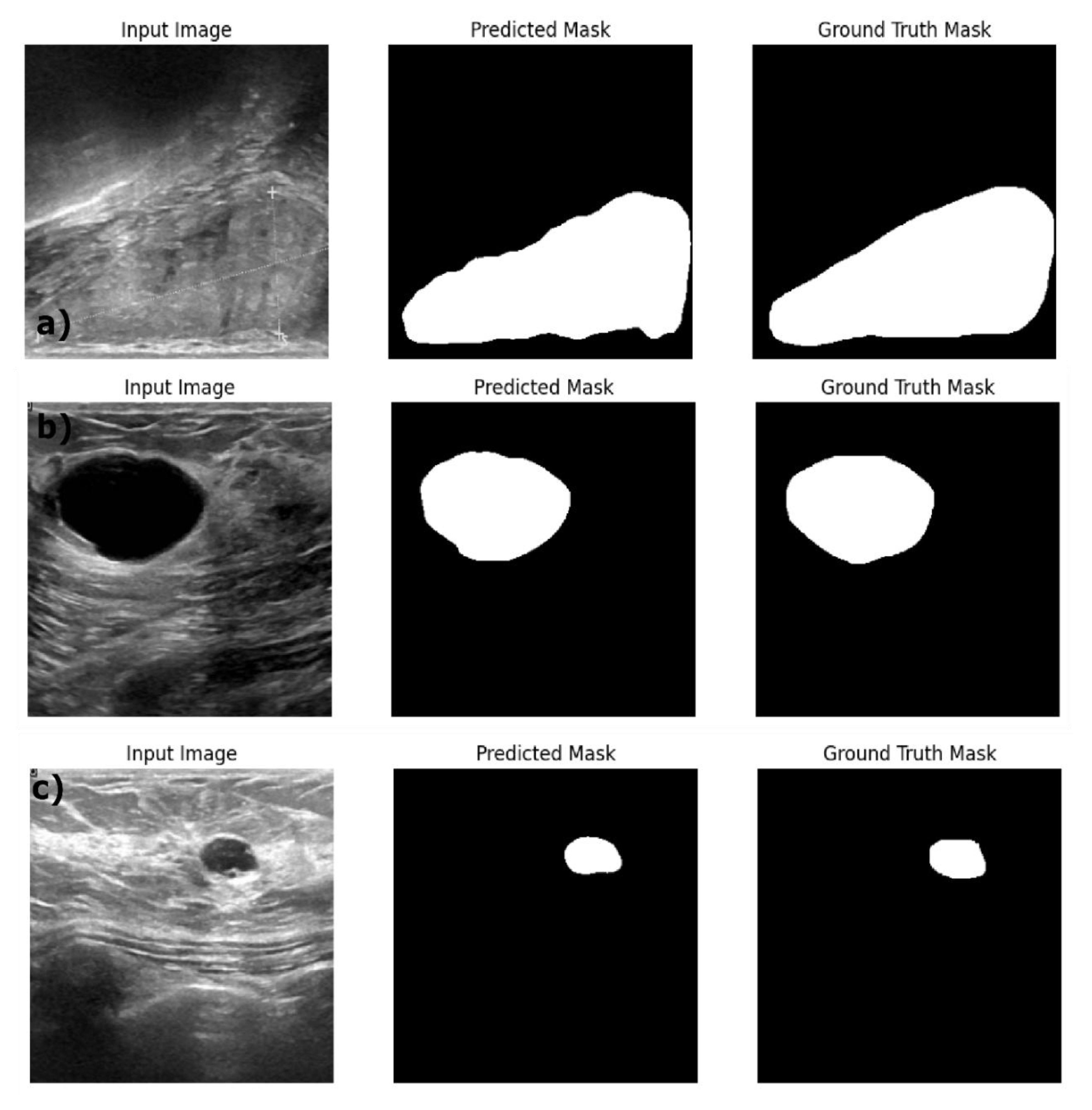
Figure 4 provides the sample results of the ResNet18:U-Net++ architecture on the train (a), validation (b) and test datasets (c); and Figure 4, illustrates that the ResNet18:U-Net++ model accurately segments across different sizes and shapes. ResNet18: DeepLabV3 model yielded the highest performance overall, with pixel accuracy of 0.98 on both training and test data sets. The Dice coefficient on the train, validation and test datasets are 0.87, 0.80 and 0.83 respectively. The ResNet18:DeepLabV3 outperformed ResNet18: U-Net++ in terms of Dice coefficients and IoU on training dataset. Also, the ResNet18: DeepLabV3 maintained high accuracy on test data, and it achieved highest Dice coefficient and IoU indicating that ResNet18: DeepLabV3 generalizes better on validation data than other developed models. Our ResNet18:DeepLabV3 results align with results reported in the literature, Badawy et al., reported a mean IoU value of 0.49 before applying fuzzy logic preprocessing (Badawy et al., 2021), our best segmentation model (ReseNet18:DeepLabV3) showed a mean IoU of 0.7. Similarly, they reported the developed U-net model has a mean IoU of 0.49 while the U-net model we developed has a mean IoU of 0.65. From figure 5, it is evident that the DeepLabV3 has striking balance between the robustness and precision in segmenting large irregular shaped lesions, medium and small lesions with high accuracy and detailed delineation of the edges.
Figure 5.
Example predictions of the ground truth mask by Resent 18: DeepLabV3 model on a) Train dataset, b) Validation dataset and c) Test dataset.
Figure 5.
Example predictions of the ground truth mask by Resent 18: DeepLabV3 model on a) Train dataset, b) Validation dataset and c) Test dataset.
4.2. Image Classification
From Table 5, you can see the results of OPTUNA optimization framework obtained for models ResNet18, InceptionV3, DenseNet121, GoogleNet and MobilenetV3 models for multiclass classification task. In the optimization process, the F1 macro score have been used to assess the models during optimization process.
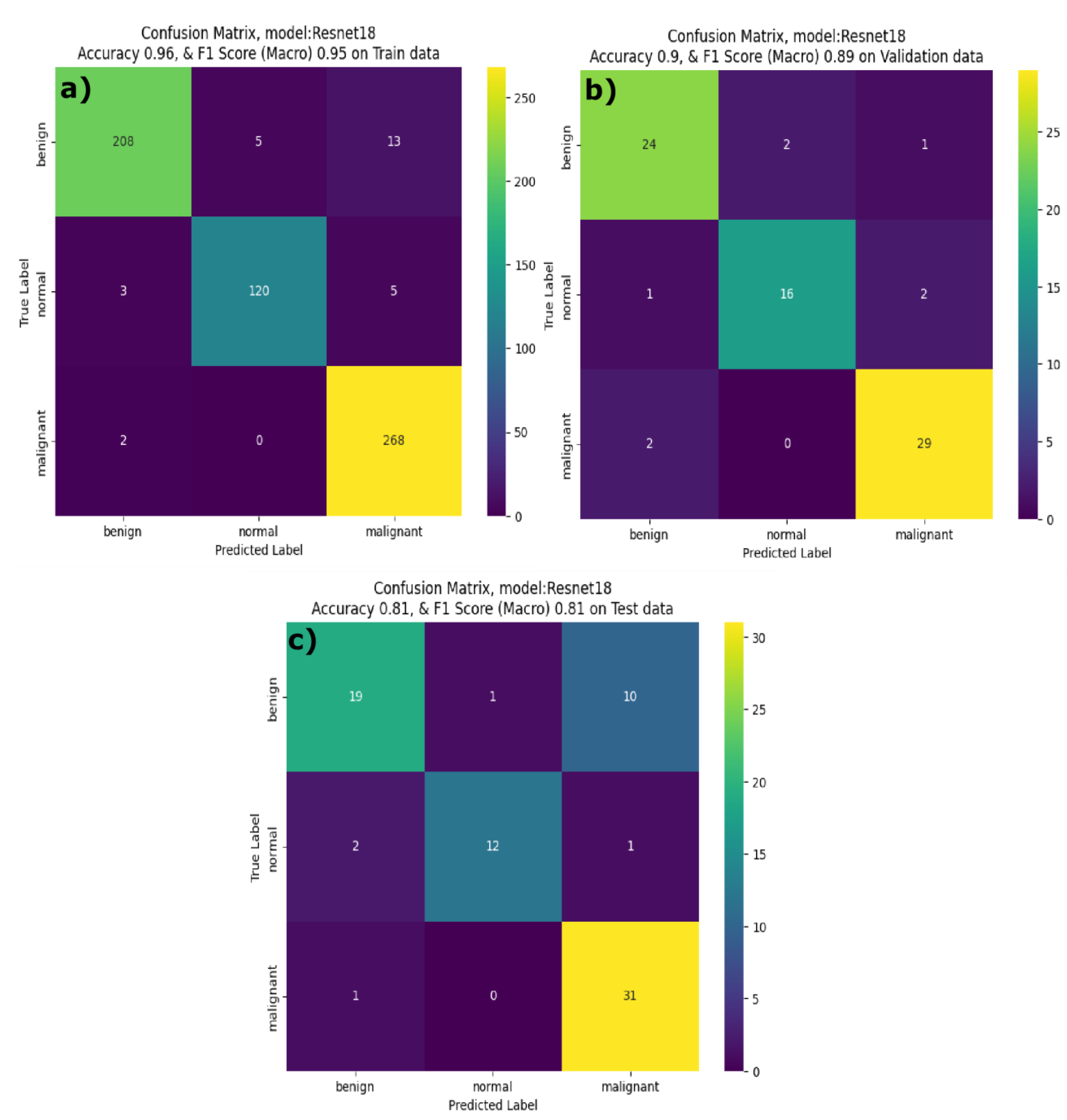
The ResNet18 has lowest F1 score of 0.77 during optimization process, while utilizing RMSprop optimizer in combination with a learning rate of 0.0000491 and weight decay 0.00027 on a training batch size of 32. GoogleNet, optimized with a adam optimizer, a, learning rate of 0.000163, weight decay of 0.00009, and a focal loss parameters α and γ equal to 0.73 and 4.24, β1 = 0.91 and β2= 0.93 achieved a slightly better F1-score of 0.82. On the other hand, InceptionV3 achieved a similar performance as GoogleNet with only one point increase in the F1 score. During optimization process, MobileNetV3 showed best F1 score 0.88 and outperformed other models. The MobileNetV3 is optimized with RMSProp and learning rate 0.0000246, weight decay 0.00060, FL(α) = 0.44 and FL(γ) = 4.86 and β1 and β2 values equal to 0.81 and 0.96 respectively. The effective performance of the AdamW for MobileNetV3 highlights the model compatibility with robust weight decay, contributing to generalization while minimizing the overfitting. Optuna optimization results revealed that optimal hyperparameters vary significantly by model architecture and MobileNetV3 achieved highest accuracy with the lowest batch size of 8 on both training and validation datasets. ResNet18 achieved a better performance on the training dataset with F1score of 0.95, accuracy of 0.90 and well-balanced precision and recall across all classes for the training dataset. ResNet18 validation performance was also high with an F1 score of 0.89 and accuracy of 0.82. However, the model’s performance on the test dataset is dropped with F1 score = 0.81 and accuracy = 0.77. Moreover, the recall on the benign class is 0.63 indicating that while ResNet18 is generalized well, it had difficulty recognizing benign classes in the test dataset. By observing the confusion matrix results (figure 6) of the ResNet18, you can see that the model correctly identified 208 benign, 120 normal and 268 malignant samples with fewer misclassifications during training phase. ResNet18 misclassified only two malignant cases in the training and validation dataset. However, during inference phase, resenet18 misclassified 10 benign cases as malignant even though it showed better performance for normal and malignant classes. Badawy et al., developed ResNet101, when compared to the light weight ResNet18 model we developed in this study, we chose the ReseNet18 due to memory constraints of the GPU we used in this study. Badawy et al., reported that ResNet101 has better performance on the BUSI dataset than that of the other ResNet variants they tested (ResNet18, ResNet50) [41].
Figure 6.
Confusion matrix of Resent18 Breast Cancer classifier on a) Train dataset, b) Validation dataset and c) Test dataset.
Figure 6.
Confusion matrix of Resent18 Breast Cancer classifier on a) Train dataset, b) Validation dataset and c) Test dataset.
The InceptionV3 model achieved an F1 score of 0.91 and an accuracy of 0.91 on the training data with a high recall in the normal class (0.99), see Table 6. On the validation dataset, InceptionV3 showed a F1 score of 0.86 with a validation accuracy of 0.74, indicating a moderate overfitting problem. During inference phase, InceptionV3 showed lower performance with a F1 score and accuracy of 0.75 and 0.83 respectively. InceptionV3 performed well on the class label normal with a precision = 1.0 but the recall for the benign class is equal to 0.63, indicating that InceptionV3 struggles to differentiate the benign class during inference phase. By observing the confusion matrix in Figure 7 the InceptionV3 model correctly identified 182 benign, 117 normal and 272 malignant cases with minimal misclassification on training dataset. From the validation data confusion matrix for the InceptionV3 model, illustrates that the model has correctly classified 36 out of 38 malignant cases. Yet during the inference phase, it faced challenges in classifying benign class with only 14 of the benign cases classified correctly and processed 7 cases where it misclassified benign samples as malignant samples. DenseNet121 performed reasonably well on the training and test (unseen) datasets. On the training dataset DenseNet121 model achieved a F1 score and accuracy of 0.86 and 0.85 respectively. On the validation dataset it achieved a F1 score of 0.73 and accuracy of 0.71 respectively. However, the model demonstrated strong performance on the test data when compared to validation data indicating that model generalizes well when applied to the unseen dataset. Examining the confusion matrix (Figure 8a) of DenseNet121 model on the training dataset, it is evident that DenseNet121 correctly identified 283 benign, 100 normal and 153 malignant samples. Although, DenseNet121 misclassified 27 benign images as normal and 40 benign samples as malignant. In the validation dataset (figure 8b), DenseNet121 showed a mixed performance with 25 benign images correctly classified, and the model misclassified 5 benign samples as normal and 6 malignant samples as normal. During the inference phase, the DenseNet121 model achieved better performance with only few misclassified samples. It correctly classified 19 benign, 17 normal and 33 malignant samples, implying high level of generalization.
The MobileNetV3 model presented consistent performance across all classes with precision and recall being above 0.9 for the training dataset. The accuracy and F1 score on the training dataset are 0.93 and 0.94 respectively. However, the MobileNetV3 model showed poor performance on the test dataset with a lower F1 score and accuracy, due to the impact of lower precision for benign class. This indicates that the MobilenetV3 model struggled to classify the benign class on the unseen dataset. The results of the developed MobileNetV3 model align with other reports in the literature. Yan et al reported that MobileNetV1 has better classification performance than that of the MobileNetV2 [40]. From Figure 9a, it is evident that the developed MobileNetV3 model correctly identified 168 benign, 129 normal and 292 malignant cases correctly. It showed strong performance on validation data (figure 9b) for benign and malignant classes. However, in the inference phase, the MobileNetV3 model misclassified 1 benign case as normal, 7 normal cases as benign, and 11 normal cases as malignant, showing confusion primarily in distinguishing the normal class.
The GoogleNet model aka InceptionV1model showed high training F1-score and accuracy scores of 0.91 and 0.91, respectively. Yet, the recall for benign cases was relatively low at 0.8 implying that model struggles to detect benign features during the training phase. The F1-score and accuracy of the GoogleNet model on the validation dataset is 0.73 and 0.73 respectively. During inference phase, GoogleNet achieved a F1 score of 0.77 and accuracy of 0.77 with a balanced precision across all the classes but lower recall for normal and malignant classes. Thus, the GoogleNet model was unable to differentiate the classes during the inference. Similarly, by observing the confusion matrix results of the GoogleNet model on train dataset, it is evident that, model showed a balanced performance across all the classes in the training phase (Figure 10a), it correctly classified 168 benign. 129 normal and 268 malignant cases with a minimal misclassification. On the validation dataset, GoogleNet correctly classified 18 benign, 17 normal and 21 malignant samples, however some of the malignant samples are misclassified as normal (Figure 10b). During inference phase, the GoogleNet model’s performance has slightly reduced, with 20 benign, 10 normal and 30 malignant cases correctly identified. However, it misclassified 7 benign cases as malignant, 3 normal cases as benign and 2 malignant classes as normal. Figure 11 shows the comparison of all developed models’ performance on train data, validation and test datasets.
Figure 11 illustrates that the ResNet18 and GoogleNetV3 models achieved the highest F1 scores on training data with GoogleNetV3 having a slightly higher F1-score of 0.93 and an accuracy of 0.91. However, the ResNet18 model demonstrated better generalization on the unseen dataset attaining validation and test accuracies of 0.82 and 0.81 respectively. InceptionV3 also performed well while DenseNet121 displayed moderate scores on validation and test F1 score of 0.73 and 0.82, respectively. Similarly, the MobileNetV3 model, despite a better training accuracy of 0.94 did not show robust performance on the test data with lower accuracy of 0.71. Considering the accuracies and F1 scores, the ResNet18 model can be selected as the most balanced model with stable performance across training, validation and test datasets. The model’s consistency of the accuracy and F1-scores across three datasets supports its reliability for the multiclass classification of breast cancer ultrasound imagery data. Sample predictions of the developed classification models is provided in the Figure 12.
5. Conclusions
With an aim of assisting the healthcare practitioners and radiologist in early detection of breast cancer, we conducted an extensive study on the application of transfer learning techniques based on the pretrained models to accurately conduct breast cancer segmentation and classification of breast cancer ultrasound images. We focused on the data augmentation, hyperparameter optimization with Optuna, and the construction of a robust training process to address challenges presented by the limited size and class imbalance of BUSI dataset. For the image segmentation task, the DeepLabV3 model outperformed U-Net and U-Net++ models by achieving high pixel accuracy and good generalization on training, validation and test datasets. U-Net predictions showed edge irregularities and over segmentation while the ResNet18: DeepLabV3 model showed strong performance in terms of delineating both large and small lesions with minimal edge irregularities. Thus, indicating the model’s suitability for breast cancer image segmentation. The DeepLabV3 ResNet18 model possessed a Dice Coefficient of 0.83, IoU of 0.71 and pixel accuracy of 0.98 on the test dataset, demonstrating its ability to generalize well on the unseen dataset. For the image classification of breast cancer images, ResNet18 model achieved an F1-score of 0.81 and an overall pixel accuracy of 0.77 on the test dataset and ResNet18 showed better generalization on the unseen dataset when compared to MobileNetV3 and GoogleNet. The MobileNetV3 model achieved highest F1-score of 0.94 on the training data but showed low accuracy (0.71) on the test data.
Author Contributions
K.E. ArunKumar: Conceptualization, Methodology, Software, Validation, Formal analysis, Writing - original draft, Visualization, Data curation and preprocessing. Matthew E Wilson: Conceptualization, Methodology, Project administration, Resources, Writing - review & editing. Nathan E. Blake: Writing - review & editing, Data curation, Tylor Yost: Writing - review & editing, Matthew Walker: Writing - review & editing, Data curation.
Funding
This research is not supported by specific grant from funding agencies in the public, commercial or non-profit organization.
References
- American Cancer Society (2024). Breast Cancer facts & figures 2024. https://www.cancer.org/content/dam/cancer-org/research/cancer-facts-and-statistics/breast-cancer-facts-and-figures/2024/breast-cancer-facts-and-figures-2024.
- . Trepanier C, Huang A, Liu M, Ha R. Emerging uses of artificial intelligence in breast and axillary ultrasound. Clinical Imaging. 2023 Aug 1; 100:64-8. [CrossRef]
- Sree SV, Ng EY, ACHARYA U RA, Tan W. Breast imaging systems: a review and comparative study. Journal of Mechanics in Medicine and Biology. 2010 Mar;10(01):5-34. [CrossRef]
- Zhang Y, Xian M, Cheng HD, Shareef B, Ding J, Xu F, Huang K, Zhang B, Ning C, Wang Y. BUSIS: a benchmark for breast ultrasound image segmentation. InHealthcare 2022 Apr 14 (Vol. 10, No. 4, p. 729). MDPI. [CrossRef]
- Bi WL, Hosny A, Schabath MB, Giger ML, Birkbak NJ, Mehrtash A, Allison T, Arnaout O, Abbosh C, Dunn IF, Mak RH. Artificial intelligence in cancer imaging: clinical challenges and applications. CA: a cancer journal for clinicians. 2019 Mar;69(2):127-57. [CrossRef]
- Kayalibay B, Jensen G, van der Smagt P. CNN-based segmentation of medical imaging data. arXiv:1701.03056. 2017 Jan 11. [CrossRef]
- Liu F, Lin G, Shen C. CRF learning with CNN features for image segmentation. Pattern Recognition. 2015 Oct 1;48(10):2983-92. [CrossRef]
- Sharma P, Berwal YP, Ghai W. Performance analysis of deep learning CNN models for disease detection in plants using image segmentation. Information Processing in Agriculture. 2020 Dec 1;7(4):566-74. [CrossRef]
- Dolz J, Gopinath K, Yuan J, Lombaert H, Desrosiers C, Ayed IB. HyperDense-Net: a hyper-densely connected CNN for multi-modal image segmentation. IEEE transactions on medical imaging. 2018 Oct 30;38(5):1116-26. 10.1109/TMI.2018.2878669.
- Hooley RJ, Scoutt LM, Philpotts LE. Breast ultrasonography: state of the art. Radiology. 2013 Sep;268(3):642-59. [CrossRef]
- Ronneberger O, Fischer P, Brox T. U-net: Convolutional networks for biomedical image segmentation. InMedical image computing and computer-assisted intervention–MICCAI 2015: 18th international conference, Munich, Germany, October 5-9, 2015, proceedings, part III 18 2015 (pp. 234-241). Springer International Publishing. [CrossRef]
- Long J, Shelhamer E, Darrell T. Fully convolutional networks for semantic segmentation. InProceedings of the IEEE conference on computer vision and pattern recognition 2015 (pp. 3431-3440). [CrossRef]
- Tai XC, Liu H, Chan RH, Li L. A mathematical explanation of UNet. arXiv:2410.04434. 2024 Oct 6. [CrossRef]
- Zhou, Z. , Rahman Siddiquee, M.M., Tajbakhsh, N., Liang, J. (2018). UNet++: A Nested U-Net Architecture for Medical Image Segmentation. In: Stoyanov, D., et al. Deep Learning in Medical Image Analysis and Multimodal Learning for Clinical Decision Support. DLMIA ML-CDS 2018 2018. Lecture Notes in Computer Science(), vol 11045. Springer, Cham. [CrossRef]
- Lee CY, Xie S, Gallagher P, Zhang Z, Tu Z. Deeply supervised nets. InArtificial intelligence and statistics 2015 Feb 21 (pp. 562-570). Pmlr. 10.48550/arXiv.1409.5185.
- He K, Zhang X, Ren S, Sun J. Deep residual learning for image recognition. InProceedings of the IEEE conference on computer vision and pattern recognition 2016 (pp. 770-778). [CrossRef]
- Szegedy C, Liu W, Jia Y, Sermanet P, Reed S, Anguelov D, Erhan D, Vanhoucke V, Rabinovich A. Going deeper with convolutions. InProceedings of the IEEE conference on computer vision and pattern recognition 2015 (pp. 1-9). 10.1109/CVPR.2015.7298594.
- Lin, M. Network in network. arXiv:1312.4400. 2013. [CrossRef]
- Yuesheng F, Jian S, Fuxiang X, Yang B, Xiang Z, Peng G, Zhengtao W, Shengqiao X. Circular fruit and vegetable classification based on optimized GoogLeNet. IEEE Access. 2021 Aug 16;9:113599-611. 10.1109/ACCESS.2021.3105112.
- Meena G, Mohbey KK, Kumar S. Sentiment analysis on images using convolutional neural networks-based Inception-V3 transfer learning approach. International journal of information management data insights. 2023 Apr 1;3(1):100174. [CrossRef]
- Wang C, Chen D, Hao L, Liu X, Zeng Y, Chen J, Zhang G. Pulmonary image classification based on inception-v3 transfer learning model. IEEE Access. 2019 Oct 7;7:146533-41. r 10.1109/ACCESS.2019.2946000.
- Howard A, Sandler M, Chu G, Chen LC, Chen B, Tan M, Wang W, Zhu Y, Pang R, Vasudevan V, Le QV. Searching for mobilenetv3. InProceedings of the IEEE/CVF international conference on computer vision 2019 (pp. 1314-1324). [CrossRef]
- Bello A, Ng SC, Leung MF. Skin Cancer Classification Using Fine-Tuned Transfer Learning of DENSENET-121. Applied Sciences. 2024 Aug 31;14(17):7707. [CrossRef]
- Soulami KB, Kaabouch N, Saidi MN, Tamtaoui A. Breast cancer: One-stage automated detection, segmentation, and classification of digital mammograms using UNet model based-semantic segmentation. Biomedical Signal Processing and Control. 2021 Apr 1;66:102481. 10.1016/j.bspc.2021.102481.
- He Q, Yang Q, Xie M. HCTNet: A hybrid CNN-transformer network for breast ultrasound image segmentation. Computers in Biology and Medicine. 2023 Mar 1;155:106629. 10.1016/j.compbiomed.2023.106629.
- Huang Q, Huang Y, Luo Y, Yuan F, Li X. Segmentation of breast ultrasound image with semantic classification of superpixels. Medical Image Analysis. 2020 Apr 1; 61:101657. 10.1016/j.media.2020.101657.
- Guo Y, Duan X, Wang C, Guo H. Segmentation and recognition of breast ultrasound images based on an expanded U-Net. Plos one. 2021 Jun 15;16(6):e0253202. [CrossRef]
- Nastase IA, Moldovanu S, Moraru L. Deep learning-based segmentation of breast masses using convolutional neural networks. InJournal of Physics: Conference Series 2024 Feb 1 (Vol. 2701, No. 1, p. 012005). IOP Publishing. 10.1088/1742-6596/2701/1/012005.
- Samudrala S, Mohan CK. Semantic segmentation of breast cancer images using DenseNet with proposed PSPNet. Multimedia Tools and Applications. 2024 May;83(15):46037-63. 10.1007/s11042-023-17411-5.
- Uysal F, Köse MM. Classification of breast cancer ultrasound images with deep learning-based models. Engineering Proceedings. 2022 Dec 2;31(1):8. [CrossRef]
- Zakareya S, Izadkhah H, Karimpour J. A new deep-learning-based model for breast cancer diagnosis from medical images. Diagnostics. 2023 Jun 1;13(11):1944. [CrossRef]
- Sivagami S, Chitra P, Kailash GS, Muralidharan SR. Unet architecture based dental panoramic image segmentation. In2020 International Conference on Wireless Communications Signal Processing and Networking (WiSPNET) 2020 Aug 4 (pp. 187-191). IEEE. 10.1109/WiSPNET48689.2020.9198370.
- Hatamizadeh A, Tang Y, Nath V, Yang D, Myronenko A, Landman B, Roth HR, Xu D. Unetr: Transformers for 3d medical image segmentation. InProceedings of the IEEE/CVF winter conference on applications of computer vision 2022 (pp. 574-584). [CrossRef]
- Al-Dhabyani W, Gomaa M, Khaled H, Fahmy A. Dataset of breast ultrasound images. Data in brief. 2020 Feb 1; 28:104863. [CrossRef]
- Dumoulin V, Visin F. A guide to convolution arithmetic for deep learning. arXiv:1603.07285. 2016 Mar 23. [CrossRef]
- Chen, LC. Rethinking atrous convolution for semantic image segmentation. arXiv:1706.05587. 2017. [CrossRef]
- Ross TY, Dollár GK. Focal loss for dense object detection. Inproceedings of the IEEE conference on computer vision and pattern recognition 2017 Jul (pp. 2980-2988). https://doi.org/10.48550/arXiv.1708.02002. [CrossRef]
- Badawy SM, Mohamed AE, Hefnawy AA, Zidan HE, GadAllah MT, El-Banby GM. Automatic semantic segmentation of breast tumors in ultrasound images based on combining fuzzy logic and deep learning—A feasibility study. PloS one. 2021 May 20;16(5):e0251899. [CrossRef]
- Said Y, Alsheikhy AA, Shawly T, Lahza H. Medical images segmentation for lung cancer diagnosis based on deep learning architectures. Diagnostics. 2023 Feb 2;13(3):546. 10.3390/diagnostics13030546.
- Yan, J. Study for Performance of MobileNetV1 and MobileNetV2 Based on Breast Cancer. arXiv:2308.03076. 2023 Aug 6. [CrossRef]
- Badawy SM, Mohamed AE, Hefnawy AA, Zidan HE, GadAllah MT, El-Banby GM. Classification of Breast Ultrasound Images Based on Convolutional Neural Networks-A Comparative Study. In2021 International Telecommunications Conference (ITC-Egypt) 2021 Jul 13 (pp. 1-8). IEEE. 10.1109/ITC-Egypt52936.2021.9513972.
- Akiba T, Sano S, Yanase T, Ohta T, Koyama M. Optuna: A next-generation hyperparameter optimization framework. InProceedings of the 25th ACM SIGKDD international conference on knowledge discovery & data mining 2019 Jul 25 (pp. 2623-2631). [CrossRef]
- Almajalid R, Shan J, Du Y, Zhang M. Development of a deep-learning-based method for breast ultrasound image segmentation. In2018 17th IEEE International Conference on Machine Learning and Applications (ICMLA) 2018 Dec 17 (pp. 1103-1108). IEEE. 10.1109/ICMLA.2018.00179.
- Byra M, Jarosik P, Szubert A, Galperin M, Ojeda-Fournier H, Olson L, O’Boyle M, Comstock C, Andre M. Breast mass segmentation in ultrasound with selective kernel U-Net convolutional neural network. Biomedical Signal Processing and Control. 2020 Aug 1;61:102027. [CrossRef]
- Yap MH, Pons G, Marti J, Ganau S, Sentis M, Zwiggelaar R, Davison AK, Marti R. Automated breast ultrasound lesions detection using convolutional neural networks. IEEE journal of biomedical and health informatics. 2017 Aug 7;22(4):1218-26. 10.1109/JBHI.2017.2731873.
- Zhou, Z., Rahman Siddiquee, M. M., Tajbakhsh, N., & Liang, J. (2018). Unet++: A nested u-net architecture for medical image segmentation. In Deep Learning in Medical Image Analysis and Multimodal Learning for Clinical Decision Support: 4th International Workshop, DLMIA 2018, and 8th International Workshop, ML-CDS 2018, Held in Conjunction with MICCAI 2018, Granada, Spain, September 20, 2018, Proceedings 4 (pp. 3-11). Springer International Publishing. 10.1007/978-3-030-00889-5_1.
Figure 3.
Example predictions of the ground truth mask by Resent 18: Unet model on a) Train dataset, b) Validation dataset and c) Test dataset.
Figure 3.
Example predictions of the ground truth mask by Resent 18: Unet model on a) Train dataset, b) Validation dataset and c) Test dataset.
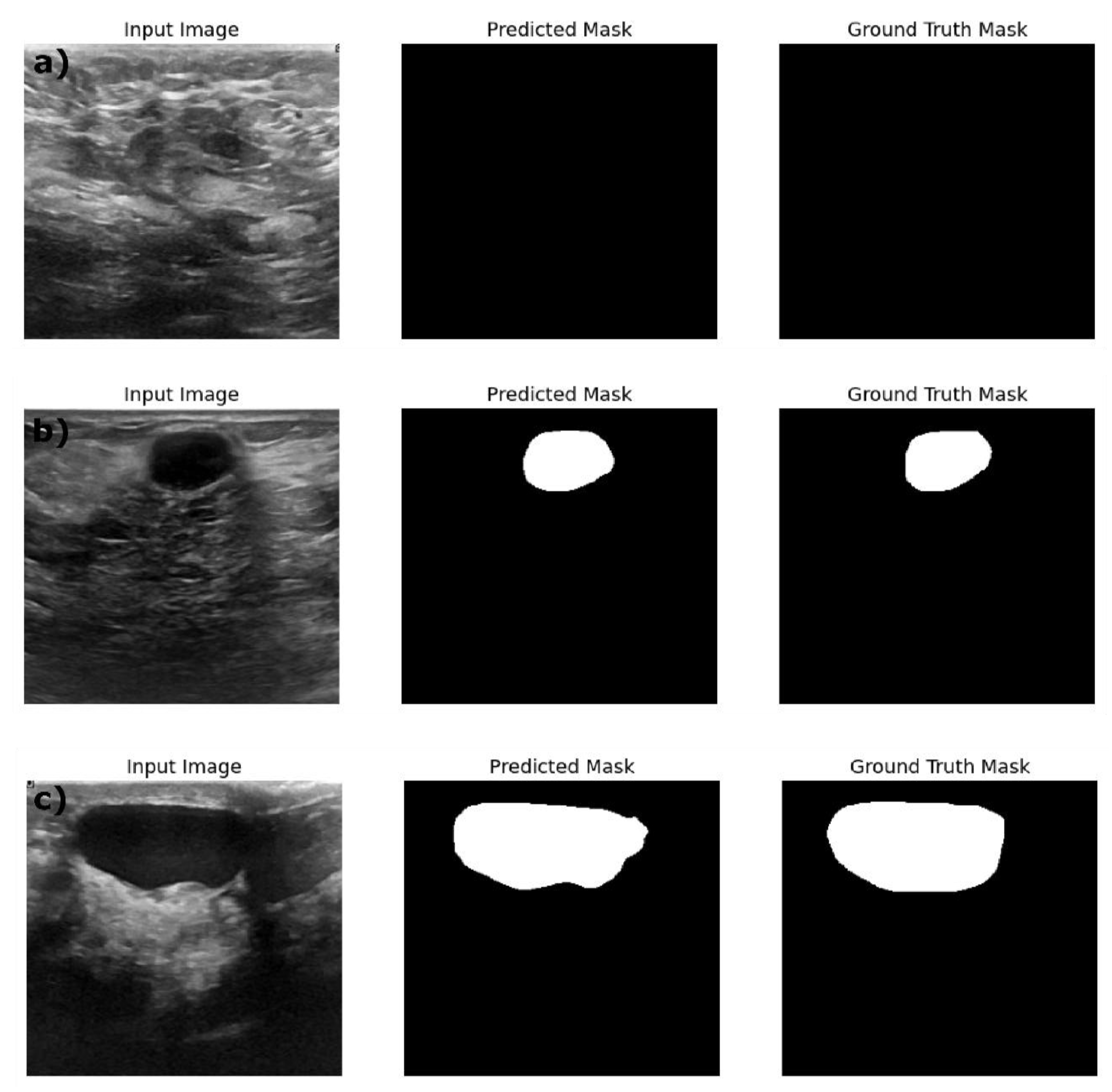
Figure 4.
Example predictions of the ground truth mask by Resent 18: Unet++ model on a) Train dataset, b) Validation dataset and c) Test dataset.
Figure 4.
Example predictions of the ground truth mask by Resent 18: Unet++ model on a) Train dataset, b) Validation dataset and c) Test dataset.
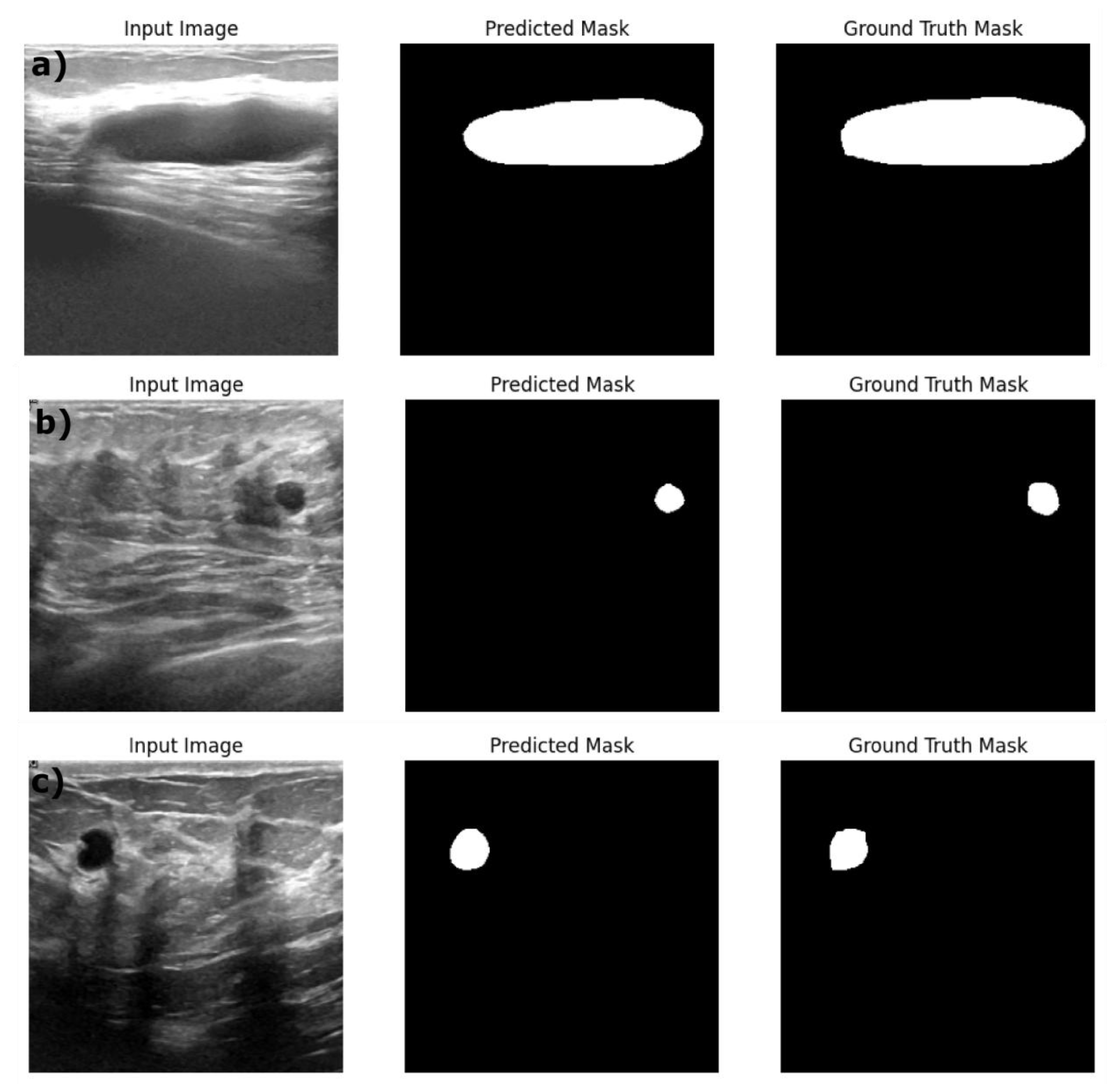
Figure 7.
Confusion matrix of InceptionV3 Breast Cancer classifier on a) Train dataset, b) Validation dataset and c) Test dataset.
Figure 7.
Confusion matrix of InceptionV3 Breast Cancer classifier on a) Train dataset, b) Validation dataset and c) Test dataset.
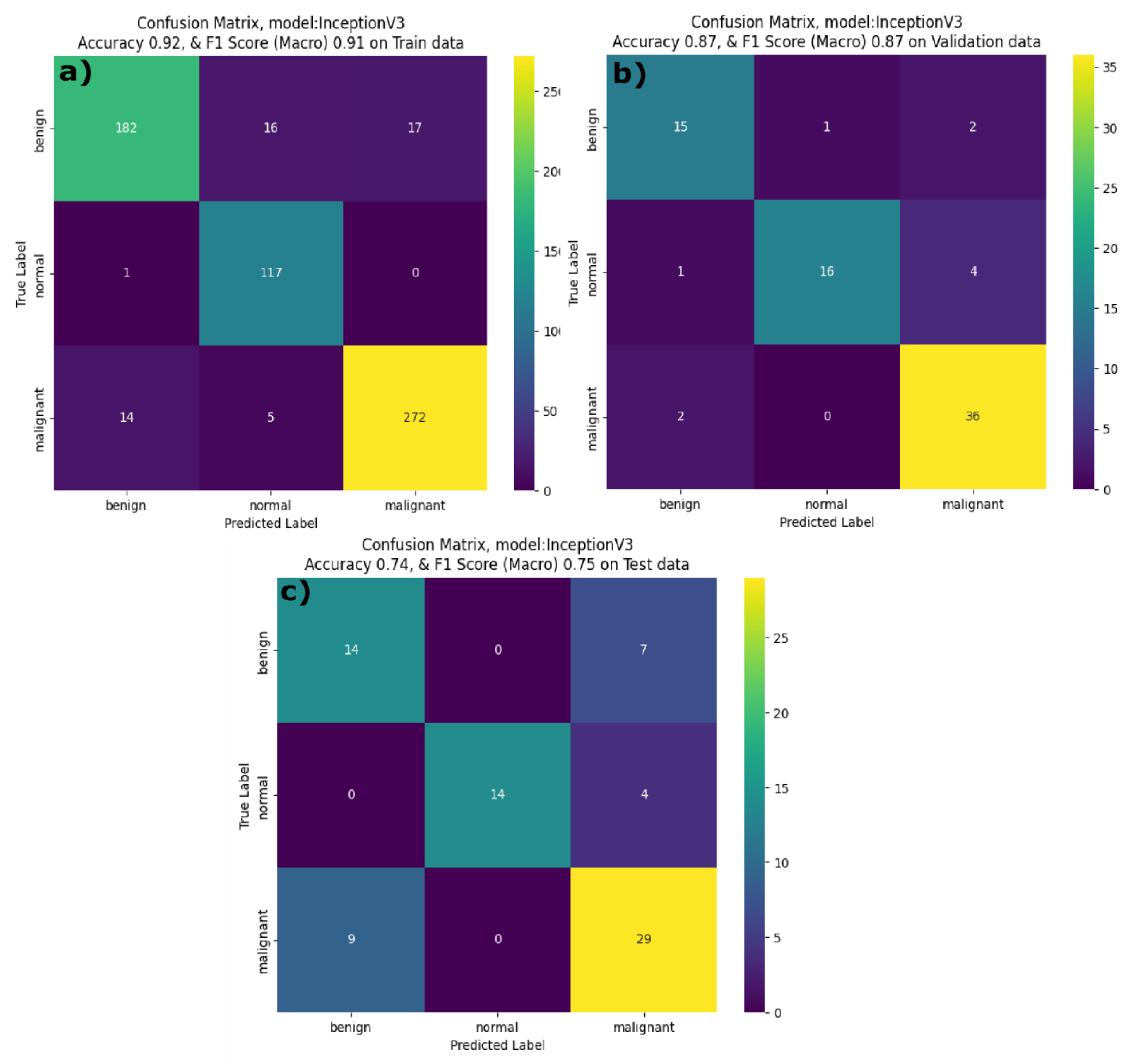
Figure 8.
Confusion matrix of Densenet121 Breast Cancer classifier on a) Train dataset, b) Validation dataset and c) Test dataset.
Figure 8.
Confusion matrix of Densenet121 Breast Cancer classifier on a) Train dataset, b) Validation dataset and c) Test dataset.
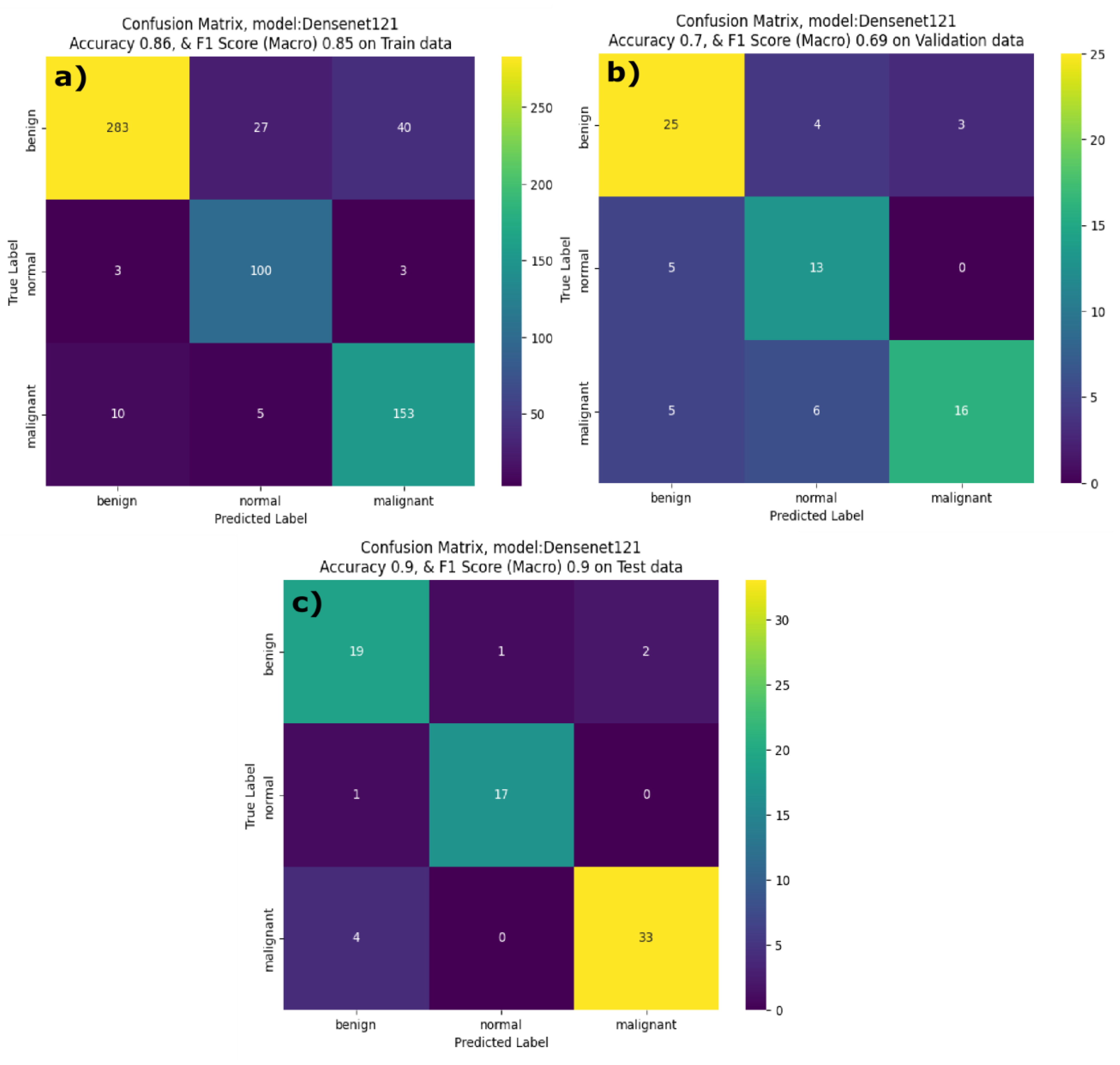
Figure 9.
Confusion matrix of MobileNetV3 Breast Cancer classifier on a) Train dataset, b) Validation dataset and c) Test dataset.
Figure 9.
Confusion matrix of MobileNetV3 Breast Cancer classifier on a) Train dataset, b) Validation dataset and c) Test dataset.
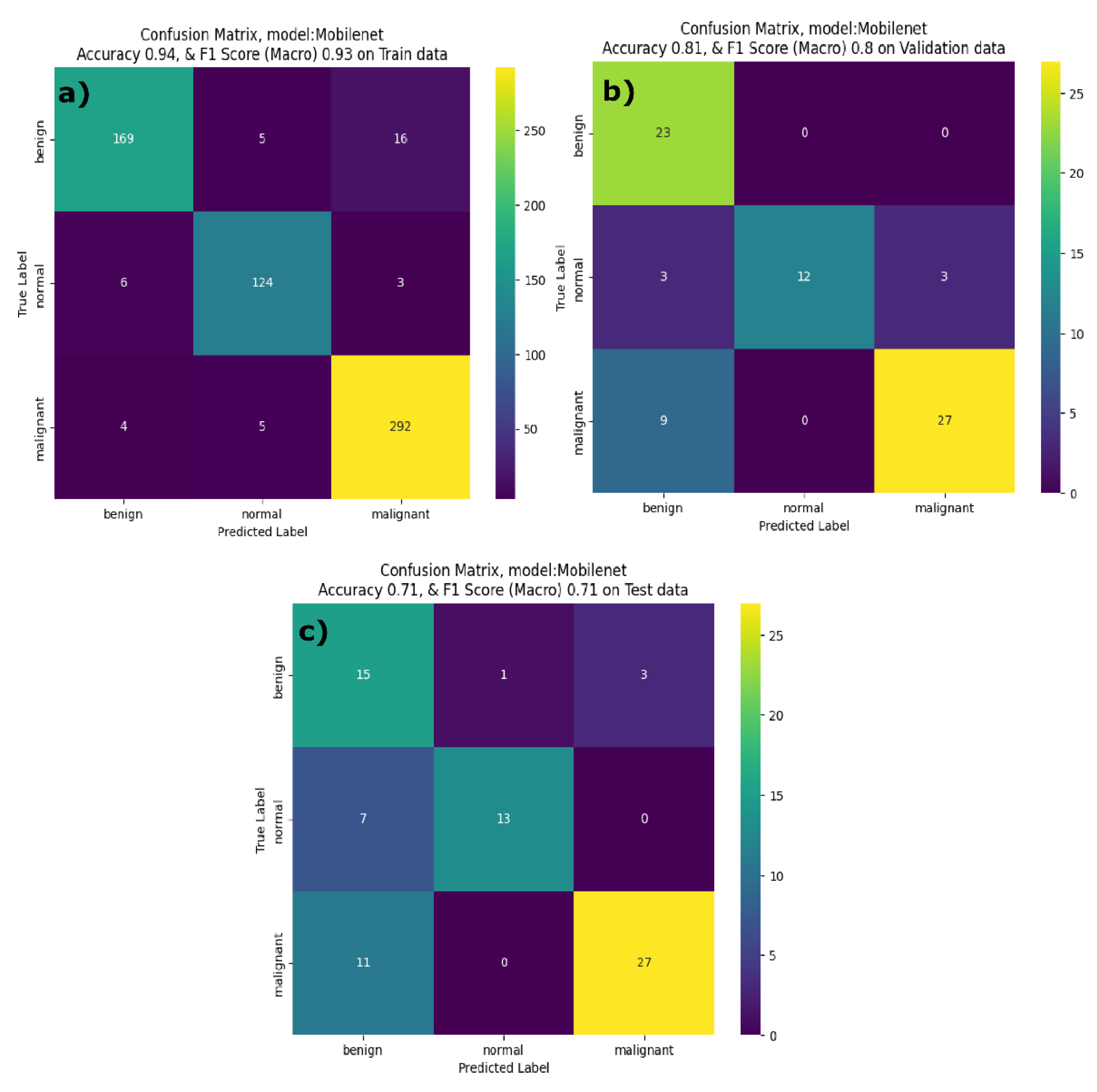
Figure 10.
Confusion matrix of GoogleNetV3 Breast Cancer classifier on a) Train dataset, b) Validation dataset and c) Test dataset.
Figure 10.
Confusion matrix of GoogleNetV3 Breast Cancer classifier on a) Train dataset, b) Validation dataset and c) Test dataset.
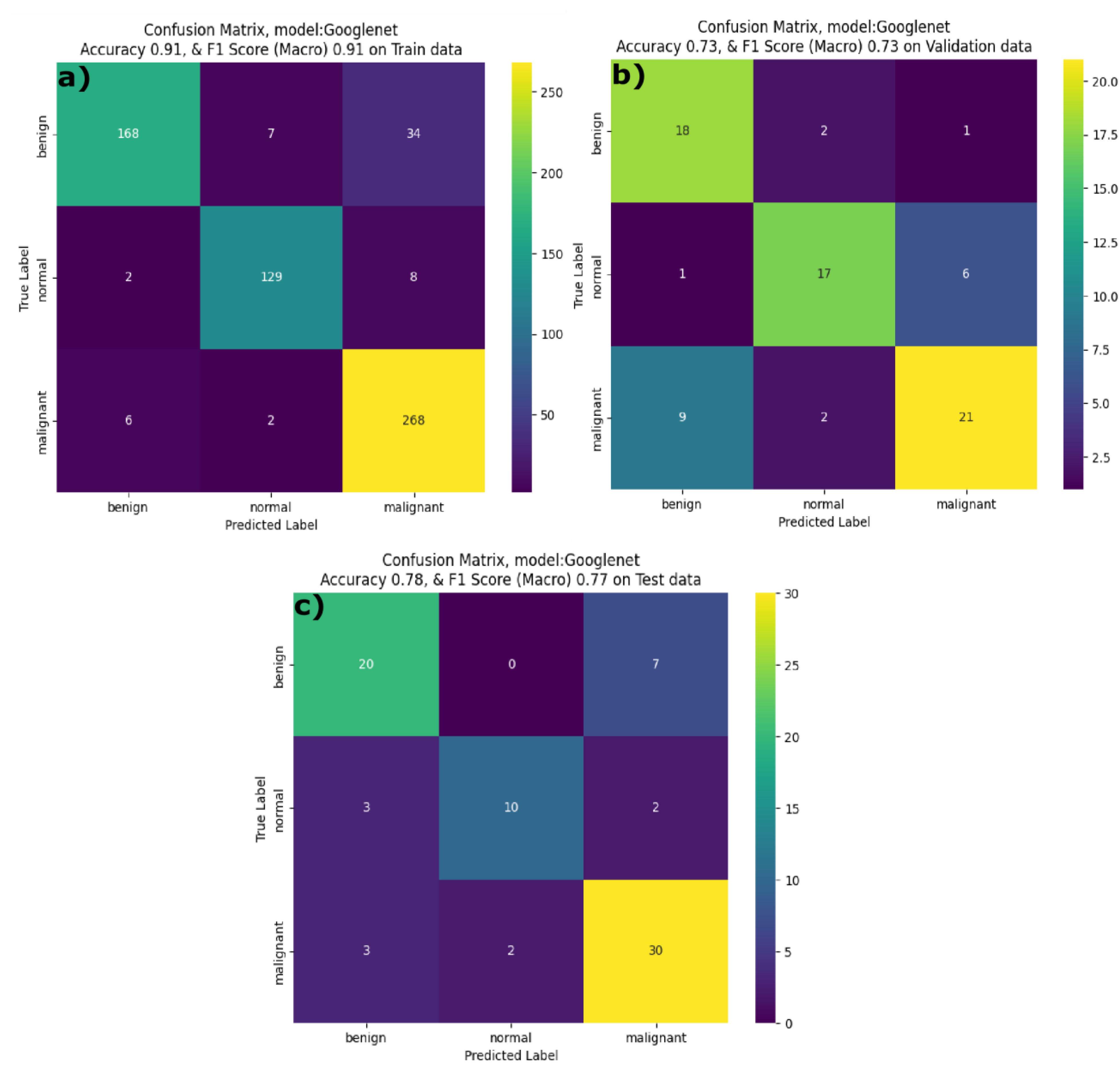
Figure 11.
Comparison of models’ performance on train, validation and test datasets based on F1 score and Accuracy.
Figure 11.
Comparison of models’ performance on train, validation and test datasets based on F1 score and Accuracy.
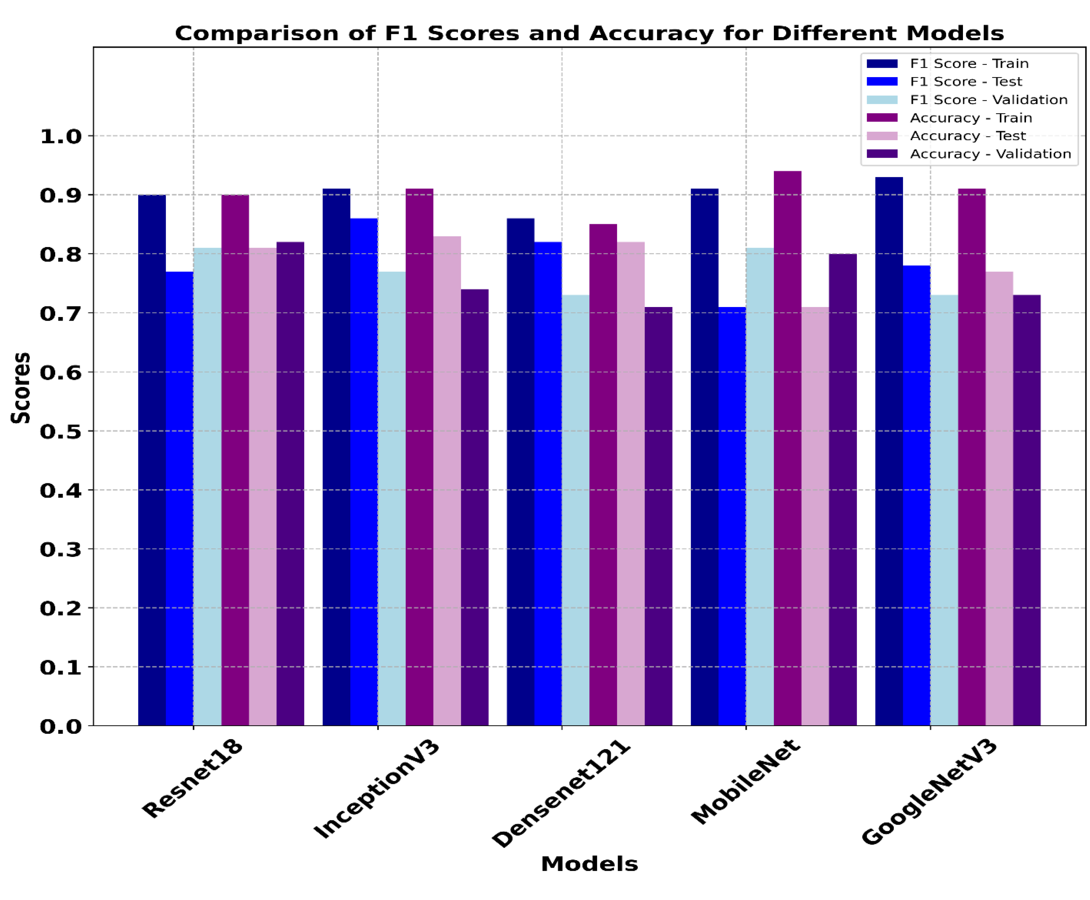
Figure 12.
Example predictions of the ground truth label (Malignant, benign and Normal) by optimized classification models developed in this study.
Figure 12.
Example predictions of the ground truth label (Malignant, benign and Normal) by optimized classification models developed in this study.
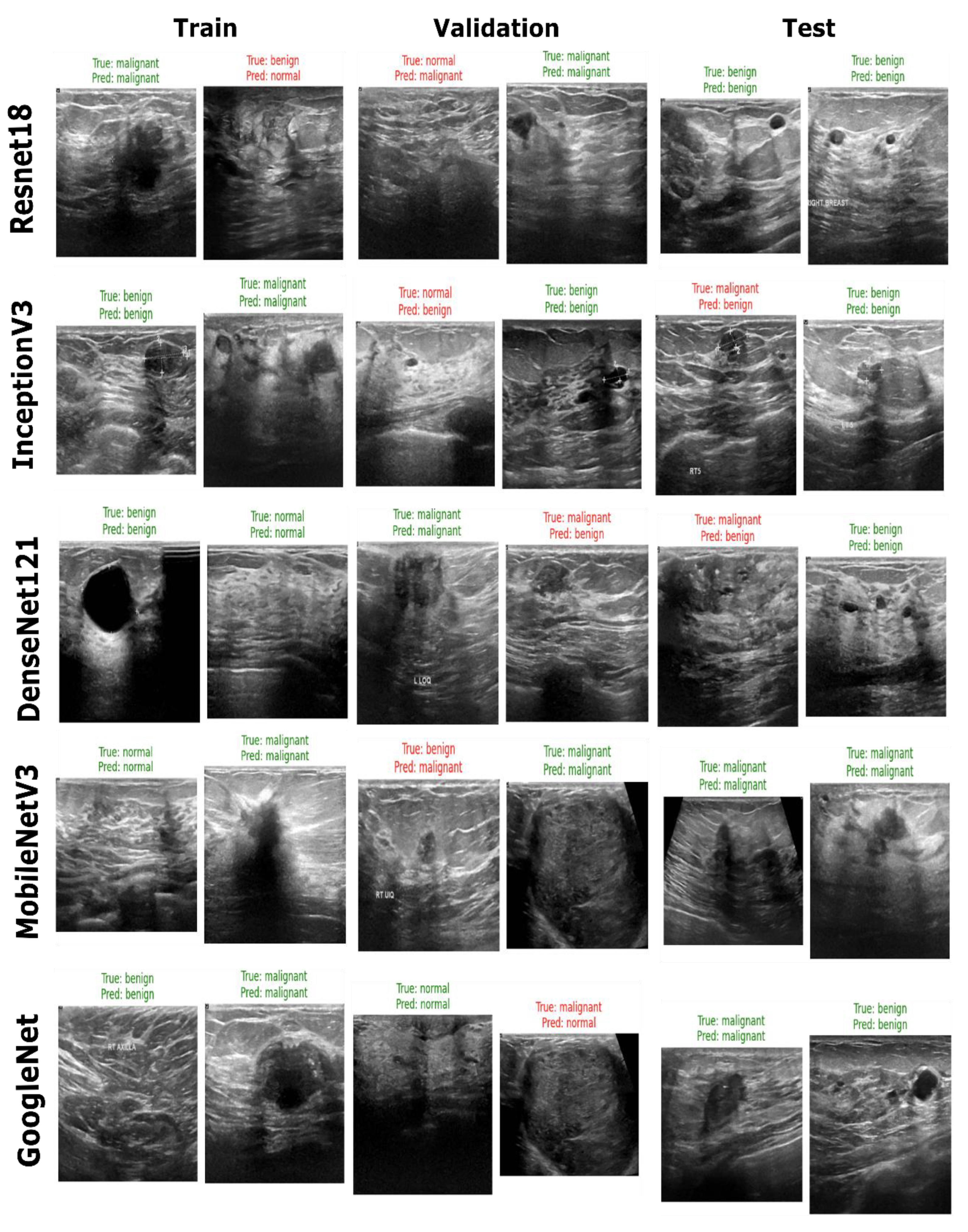
Table 3.
Optuna Hyperparameter Optimization of segmentation models.
| Encoder | Decoder | Learning rate | Weight Decay | Batch Size | Optimizer | Image size |
| Resnet18 | Unet | 0.000081 | 0.000079 | 8 | Adam | 288 |
| Resnet18 | Unet++ | 0.000155 | 1.09011 | 8 | RMSprop | 288 |
| Resnet18 | DeepLabV3 | 0.00019 | 0.00019 | 8 | AdamW | 256 |
Table 4.
Performance of Segmentation models on Training, validation and Test datasets.
| Encoder: Decoder |
Dataset |
Pixel Accuracy | Dice Coefficient | IoU | AUC score |
| Resnet18-Unet | Train | 0.97 | 0.86 | 0.76 | 0.91 |
| Validation | 0.96 | 0.76 | 0.62 | 0.85 | |
| Test | 0.96 | 0.74 | 0.59 | 0.82 | |
| Resnet18-Unet++ | Train | 0.98 | 0.87 | 0.77 | 0.92 |
| Validation | 0.96 | 0.76 | 0.60 | 0.84 | |
| Test | 0.97 | 0.83 | 0.71 | 0.91 | |
| Resnet18-DeepLabV3 | Train | 0.98 | 0.87 | 0.78 | 0.93 |
| Validation | 0.97 | 0.80 | 0.67 | 0.87 | |
| Test | 0.98 | 0.83 | 0.70 | 0.90 |
Table 5.
Optuna hyperparameter optimization of multiclass breast cancer classification models.
|
Model |
Optimizer | Learning rate | Weight Decay | FL(α)* | FL(γ)* | Batch size | β1 | β2 | F1 score |
| Resnet18 | RMSprop | 0.0000491 | 0.00027 | 0.57 | 4.03 | 32 | N/A | N/A | 0.77 |
| InceptionV3 | Adam | 0.0000163 | 0.00009 | 0.33 | 4.41 | 16 | 0.84 | 0.98 | 0.83 |
| Densenet121 | RMSprop | 0.0000246 | 0.00060 | 0.65 | 3.55 | 32 | N/A | N/A | 0.87 |
| MobilenetV3 | AdamW | 0.0001120 | 0.00626 | 0.44 | 4.86 | 8 | 0.81 | 0.96 | 0.88 |
| GoogleNet | Adam | 0.0008705 | 0.00015 | 0.73 | 4.24 | 32 | 0.91 | 0.93 | 0.82 |
*FL(α) is the weighting factor that balances different classes, when the dataset is imbalanced dataset, FL(γ) is the focusing parameter that focuses on the instances that are hard to classify.
Table 6.
Performance of the Breast Cancer classifiers on Train, Validation and Test datasets.
| Model | Dataset | F1score | Accuracy | Metric | Benign | Normal | Malignant | Macro AVG |
| Resnet18 | Train | 0.90 | 0.90 | Precision | 0.98 | 0.96 | 0.94 | 0.96 |
| Recall | 0.92 | 0.94 | 0.99 | 0.95 | ||||
| F1 score | 0.95 | 0.95 | 0.95 | 0.95 | ||||
| Test | 0.77 | 0.81 | Precision | 0.86 | 0.92 | 0.74 | 0.84 | |
| Recall | 0.63 | 0.80 | 0.97 | 0.80 | ||||
| F1 score | 0.73 | 0.86 | 0.84 | 0.81 | ||||
| Validation | 0.81 | 0.82 | Precision | 0.89 | 0.89 | 0.91 | 0.89 | |
| Recall | 0.89 | 0.84 | 0.94 | 0.89 | ||||
| F1 score | 0.89 | 0.86 | 0.92 | 0.89 | ||||
| InceptionV3 |
Train |
0.91 |
0.91 |
Precision | 0.92 | 0.85 | 0.94 | 0.90 |
| Recall | 0.85 | 0.99 | 0.93 | 0.92 | ||||
| F1 score | 0.88 | 0.91 | 0.94 | 0.91 | ||||
| Test |
0.86 | 0.83 |
Precision | 0.61 | 1.0 | 0.72 | 0.78 | |
| Recall | 0.67 | 0.78 | 0.76 | 0.74 | ||||
| F1 score | 0.64 | 0.88 | 0.74 | 0.75 | ||||
| Validation | 0.77 | 0.74 | Precision | 0.83 | 0.94 | 0.86 | 0.88 | |
| Recall | 0.83 | 0.76 | 0.95 | 0.85 | ||||
| F1 score | 0.83 | 0.84 | 0.90 | 0.86 | ||||
| Densenet121 | Train | 0.86 | 0.85 | Precision | 0.96 | 0.76 | 0.78 | 0.83 |
| Recall | 0.81 | 0.94 | 0.91 | 0.89 | ||||
| F1 score | 0.88 | 0.84 | 0.84 | 0.85 | ||||
| Test | 0.82 | 0.82 | Precision | 0.79 | 0.94 | 0.94 | 0.89 | |
| Recall | 0.86 | 0.94 | 0.89 | 0.90 | ||||
| F1 score | 0.83 | 0.94 | 0.92 | 0.90 | ||||
| Validation | 0.73 | 0.71 | Precision | 0.71 | 0.57 | 0.84 | 0.71 | |
| Recall | 0.78 | 0.72 | 0.59 | 0.70 | ||||
| F1 score | 0.75 | 0.63 | 0.70 | 0.69 | ||||
| MobileNetV3 | Train | 0.93 | 0.94 | Precision | 0.94 | 0.93 | 0.94 | 0.94 |
| Recall | 0.89 | 0.93 | 0.97 | 0.93 | ||||
| F1 score | 0.92 | 0.93 | 0.95 | 0.93 | ||||
| Test | 0.71 | 0.71 | Precision | 0.45 | 0.93 | 0.90 | 0.76 | |
| Recall | 0.79 | 0.65 | 0.71 | 0.72 | ||||
| F1 score | 0.58 | 0.76 | 0.79 | 0.71 | ||||
| Validation | 0.81 | 0.80 | Precision | 0.66 | 1.00 | 0.90 | 0.85 | |
| Recall | 1.00 | 0.67 | 0.75 | 0.81 | ||||
| F1 score | 0.79 | 0.80 | 0.82 | 0.80 | ||||
| GoogleNet | Train | 0.91 | 0.91 | Precision | 0.95 | 0.93 | 0.86 | 0.92 |
| Recall | 0.80 | 0.93 | 0.97 | 0.90 | ||||
| F1 score | 0.87 | 0.93 | 0.91 | 0.91 | ||||
| Test | 0.78 | 0.77 | Precision | 0.77 | 0.83 | 0.77 | 0.79 | |
| Recall | 0.74 | 0.67 | 0.86 | 0.75 | ||||
| F1 score | 0.75 | 0.74 | 0.81 | 0.77 | ||||
| Validation | 0.73 | 0.73 | Precision | 0.64 | 0.81 | 0.75 | 0.73 | |
| Recall | 0.86 | 0.71 | 0.66 | 0.74 | ||||
| F1 score | 0.73 | 0.76 | 0.70 | 0.73 |
Disclaimer/Publisher’s Note: The statements, opinions and data contained in all publications are solely those of the individual author(s) and contributor(s) and not of MDPI and/or the editor(s). MDPI and/or the editor(s) disclaim responsibility for any injury to people or property resulting from any ideas, methods, instructions or products referred to in the content. |
© 2025 by the authors. Licensee MDPI, Basel, Switzerland. This article is an open access article distributed under the terms and conditions of the Creative Commons Attribution (CC BY) license (http://creativecommons.org/licenses/by/4.0/).
Copyright: This open access article is published under a Creative Commons CC BY 4.0 license, which permit the free download, distribution, and reuse, provided that the author and preprint are cited in any reuse.


