
Submitted:
12 November 2025
Posted:
13 November 2025
You are already at the latest version
Abstract
Large eddy simulation (LES) within a weather research and forecasting (WRF) model coupled with an active scalar transport equation was used to simulate Atmospheric Boundary Layer (ABL) conditions during the Mosquito wildland fire, the largest wildland fire in California during September of 2022. The simulations were conducted with realistic boundary conditions derived from the NOAA High Resolution Rapid Refresh (HRRR) model, with the aim of better understanding the two-way coupling between atmospheric boundary layer (ABL) and plume dynamics. The terrain was extremely inhomogeneous and the topography varied quite significantly within the numerical domain. Initially, LES of the smoke-free ABL were conducted on nested domains, and detailed ABL data were gathered from 08-09 September, 2022. LES simulations were validated using 4 ASOS stations and NOAA-MET Twin Otter measurements and the desired accuracy has been established. The smoke plume was then released into the ABL at noon on 09 September, 2022 and the plume simulations were conducted for a period of one hour from the release. During this period, the ABL transitioned from convective to buoyancy-shear-driven regimes. Late-night and early-morning conditions are influenced by the complex topography and low-level jet, whereas buoyancy and shear control the ABL dynamics during the morning and afternoon hours. The plume vertical transport is influenced by the ABL-depth and the size of the vertical turbulence structures during that time, whereas, the wind conditions and turbulent kinetic energy within the ABL dictate the horizontal transport scales of the plume. In addition, the results demonstrate that the plume modifies the microclimate along its path.
Keywords:
scalar plume dispersion
; convective regimes
; high-resolution WRF-ARW
; passive tracers
; convective transport
; mosquito fire
1. Introduction
Wildland fires (WF) interact dynamically with the ambient atmospheric boundary layer (ABL), and the state of the ABL significantly influences the transport and mixing of the gases released from fire plumes. More importantly, the fire plume modifies the micro-climate in the region surrounding the fire. Understanding the two-way interaction between the ABL and the WF is an important and outstanding problem in atmospheric science research. With a growing number of wildland fires, both in terms of intensity and number of incidences, improving the fundamental understanding of the two-way interactions between the WF and ABL can make important contributions to the progress of atmospheric dynamics science, with implications for climate change.
It has been well established that WF create their own weather [12]. Numerical simulations[15,16,19,31] and mathematical models [1] have been used to predict behaviors, such as plume rise and, transport scales. However, predicting the dynamical interactions between the background atmospheric boundary layer and the fire plumes is extremely challenging, and most current models simplify the key physics. In Conventional fire models the fire and atmosphere couplings are not well represented for large-scale fire events [15,20,36]. Further, coupled models such as WRF-Fire [45,48] and other coupled atmosphere and fire models [18,30,33,41,42] do not account for the buoyant transport of smoke and pollutants generated by the fire. The Plume dispersion is treated as a passive scalar and hence cannot accurately account for entrainment effects due to atmospheric turbulence. This misrepresents buoyancy-generated turbulence, and hence the transport characteristics of the plume may not be accurate.
Smoke and other pollutants released from wildfires are buoyant in nature, and transport from wildfires is physically represented as a buoyant plume [11,32].Buoyant plumes released into the convective boundary layer (CBL) are significantly influenced by the dynamics of the atmospheric boundary layer (ABL). In particular, under the influence of sensible upward surface heat flux, the CBL is dominated by the competing roles of shear- and buoyancy forcings [43]. Although efforts are underway to improve the WF modeling, focusing on increasing the accuracy of WRF-Fire wildfire simulations with improved fuel mapping [34], the current framework used for WRF-Fire and other coupled models represents the plume as a passive scalar. Advancing further in this direction, a new formulation, bPlume-WRF-LES model, was implemented within the WRF Model to simulate the plume as an active scalar that interacts dynamically with the atmosphere due to the buoyancy produced from the smoke and other pollutants. This was achieved by coupling an additional transport equation for the plume gas mixture and by accounting for the buoyancy production term in the turbulence kinetic energy equation [9].
The Mosquito Wildland Fire, which began on 06 September 2022, on the western slope of the Sierra Nevada, was California’s largest wildfire of the year. The atmospheric conditions before and during the early days of the Mosquito Fire’s spread included the combination of a heat wave that produced the all-time highest temperature of 116 degrees Fahrenheit ( 320K), and vegetation moisture levels close to record lows. On 07 September, the fire grew considerably, developing a massive pyro-cumulus cloud; 08 September was the largest day of growth, as fire activity intensified and became plume-dominated, producing an enormous pyro-cumulonimbus cloud.
The California Fire Dynamics Experiment (CalFiDE) campaign was conducted during August and September 2022 to sample wild-fires in northern California and southern Oregon ([13]). The field operations were coordinated with the overpasses of the NASA Earth Observing System’s Terra satellite to obtain the regional-scale snapshots of Mosquito fire plume in the northeast of Sacramento, California using the space-based Multi-angle Imaging SpectroRadiometer (MISR) instrument [39]. The Mosquito fire was captured by MISR on 08 September around 18.49 UTC. This time corresponds to around 12pm local time in California.
The purpose of this manuscript is two-fold: First, to conduct a multi- domain, 24-hour simulation of the ABL in the Mosquito-fire region during 08-09 September, 2022, constrained by ambient meteorology, and second, to simulate for one hour the release of a fire plume during this period, under realistic ambient conditions obtained from the ABL simulations. The plume simulations were performed using a high-resolution, fine-mesh LES, so turbulence scales are captured, and were conducted for a period of 60 minutes following plume-release. The high-resolution model makes it possible to quantify ABL dynamics during fire spread and to correlate plume evolution with the ABL characteristics that influence it.
It should be noted that LES of the plume is computationally expensive and with current computational capabilities, it is possible to simulate the plume growth for a limited time, and in a smaller numerical domain than that used for the ABL simulation (See Section 2 for details). For this purpose, we first conducted WRF-LES simulation of the ABL before and during plume release, to determine the state of the ABL at each hour during this period. Using the state of the ABL as initial conditions, the plume was released into the numerical domain. This process captures the two-way interactions between the ABL and the plume as the plume spreads into the domain.
Due to the release of the plume into the atmosphere, the boundary layer characteristics, including the wind speed, wind shear, turbulent kinetic energy (TKE), turbulence production, and temperature gradient significantly influence the scales of horizontal and vertical plume transport. In addition, strong turbulent longitudinal vortices with updrafts and downdrafts originate near the ground. Thus, a vertical flux of momentum, buoyancy, and emissions is created from the WF. The horizontal transport scales of the plume are governed by the wind shear, wind strength, and the local atmospheric turbulence [3,4,7,8]. The boundary layer depth, inversion layer stability structure, and turbulence intensity in this layer influence the scales of plume vertical transport. The atmospheric stability is measured using the shear-buoyancy ratio, and the stability parameter , (where. is friction velocity, is convective velocity, is the ABL height and L is the Monin-Obukhov length scale) [21]. It is important to understand that the study of plume transport is tightly connected to the dynamics of the ABL.
In the past, the Advanced Research Version of Weather Research and Forecast (WRF-ARW) was demonstrated as an effective modeling platform to study plume transport [10,38,50,51,52]. Further, it was established that simulated meteorological data using the WRF-ARW model is comparable to the observations [2,17,50].
In the present work, the detailed atmospheric conditions in the region are simulated using a high-resolution Advanced Research version of the Weather Research Forecast Model (WRF-ARW v4.1) (hereafter WRF) [46] with realistic boundary conditions derived from the NOAA High-Resolution Rapid Refresh (HRRR) model.
As the input data for the WRF model is available at a coarser resolution, the initial and boundary conditions for the actual numerical domain are obtained using multiple nested WRF domains. The regional domain for all the cases is the Sierra Nevada region, California, United States. The plume was initialized at the center of the region ( N, W), To study the release of the plume at 12 pm local time, 09 September, 2022, high-resolution WRF-LES simulations of the ABL were conducted and the model data was gathered for the period from 06-09 September, 2022.
The objectives of this manuscript are as follows:
- To investigate the structure of the atmospheric boundary layer using WRF-LES for a 24-hour period during 08-09 September, 2022 around the plume-release location (39.006o N, 120.745o W).
- To conduct high-resolution simulations of a plume released into the ABL to investigate its impact on plume vertical and horizontal transport.
2. Methodology
2.1. Numerical Model
Large eddy simulation (LES) within a weather research and forecasting (WRF) model coupled to active scalar transport equations was developed and validated to simulate buoyant plumes [6,9]. A thorough performance assessment of the WRF-LES model has been conducted to accurately resolve the micro-scale turbulence [5,6,7,9,14]. For the sake of completeness, the numerical framework is presented briefly here. The governing equations are the compressible Euler equations with eddy viscosity and gravitational forces as follows:
where is the mixture density, is the velocity component in the i direction, is the potential temperature, is the mass fraction of m-th species, and K is the modeled TKE. p is the pressure, is the modeled stress tensor given by , is the Kronecker delta function, is the specific heat capacity at constant pressure, and is the heat flux applied at the source only. The gravitational term g is considered is the flux of the species at the surface. as a body force, which acts in the negative vertical direction. The eddy viscosity, , is defined as where and l is a length scale given as , if , otherwise . Brunt–Väisälä frequency, N, is computed as .
is the turbulent Prandtl number which is defined as . From observations, along the centerline in all plumes.
Ideal gas is assumed in the equation of state, and therefore, potential temperature can be related in the equation of state, , where R is the specific gas constant and is the specific heat ratio. In the following discussion, the horizontal and vertical velocities are presented as and . The spatial directions and , they are replaced by x and z.
Besides the small scale turbulence modeled in (??)(1e), large scale quantities, including density, velocities, temperature and mass fraction, are resolved in the conservation laws (??)(1a-1d). Note that density () is calculated based on the local mass fraction. In addition, the system simulates buoyancy effects without the Boussinesq assumption (i.e., the density is allowed to vary).
Horizontal turbulence and mixing are computed using 2nd order horizontal diffusion on model levels, whereas, the vertical mixing is evaluated from the planetary boundary layer (PBL) scheme [5]. The eddy coefficient, K, is computed using the 2-D Smagorinsky first-order closure method.
2.2. Domain Configuration
The WRF model is configured with three nested domains to conduct the ABL simulations. The physical domain is shown in Figure 1a and the computional domain is shown in Figure 1b. The topography of the domain is shown in Figure 2. In our previous studies, we tested and verified the WRF-LES model ability to simulate the ABL at scales similar to this study [5,7]. Domains D01 and D02 are nested with feedback turned “on” and were used for mesoscale simulations. The LES runs were performed in domain D03. The sizes of D01, D02 and D03 are 360 km, 103km and 34km, in the horizontal direction, respectively. The horizontal resolutions for the mesoscale domains are 3 km (D01) and 1 km (D02) and for the LES domains 333.33m is used for the ABL simulations. For all the three domains, the model top is considered at 50 hPa ( 20 km) with a total of 41 levels, including 12 levels within the ABL. The first grid point is at 24.08 m above ground. In the horizontal direction, D01 is discretized into a 120 × 120 grid, D02 into 103 × 103, and D03 into 103 × 103 grid points. The mesoscale runs are initialized at 00 UTC on 05 September, 2022, and run for a period of 4 days. Meteorological initial and boundary conditions for D01 are obtained from datasets provided by the NOAA High-Resolution Rapid Refresh (HRRR) Model. The HRRR is run operationally by NCEP’s Environmental modeling center [44] and covers the Continental United stated (CONUS) in real-time at 3-km resolution, hourly updated, cloud-resolving and including convection. Radar data are assimilated in the HRRR every 15 min over a 1-h period adding further detail to that provided by the hourly data assimilation from the 13km radar-enhanced data.
The model physics chosen in WRF are outlined in Table 1.
2.3. Meteorological Evaluation
The WRF model performance was evaluated against the hourly observations of temperature and relative humidity at 2 m, wind speed and wind direction at 10 m collected at four Automated surface observing system (ASOS) stations that are located inside D02 (Figure 3). To compensate for the lack of balloon soundings in order to perform upper-air model assessment inside D02, the wind profile data collected by the NOAA-MET Twin Otter (MET-TO) research aircraft were used. The MET-TO was equipped with Micro-pulse Doppler lidar collecting the atmospheric backscatter, vertical velocity and horizontal wind profiles. MET-TO flew over the fire area a few times between 09/08 1800 UTC to 09/09 0000 UTC and six flight legs of nearly constant altitude were chosen (Figure 4) for comparing the WRF simulated wind profiles.
The following metrics of Mean Absolute Error (MAE), Mean Bias Error (MBE), Root-Mean Square Error (RMSE), and Pearson correlation coefficient (R) were calculated for assessing the WRF model performance against ASOS observations.
where denotes the model value, is the observed value, and n represents the number of data points.
Surface meteorological fields from the WRF D02 output from 09/06 0000 UTC to 09/09 0000 UTC were used for the evaluation. The WRF grid cell corresponding to the ASOS station location was chosen based on the nearest neighbor approach. Performance metrics at individual and also averaged across all 4 ASOS stations for surface variables are shown in Tables 2 and 3. Overall, the model simulated temperature matches closely with the station observations across all 4 sites, with an average MBE of 0.02 K. Similar agreement was found with 2 m RH and 10 m wind direction fields, with an average bias of 1.36% and 3.35 deg respectively. Contrary to the wind direction, the model consistently over-predicted the wind speed at all 4 sites with an average MBE of 1.4 m/s. The wind speeds observed at the ASOS stations were weak to moderate ranging from 1-3 m/s. Given the complex terrain around the ASOS station locations, it is reasonable for the model to deviate from the observed values, especially when the winds are weak to moderate. This somewhat poor performance of the WRF model in simulating the surface winds over complex terrain was observed previously by other researchers ([28]; [47]). We assessed the sensitivity of the model performance by averaging the model output over 1-3 grid cells surrounding the ASOS station locations when comparing against the observations. However, this did not result in a significant improvement in the model performance.
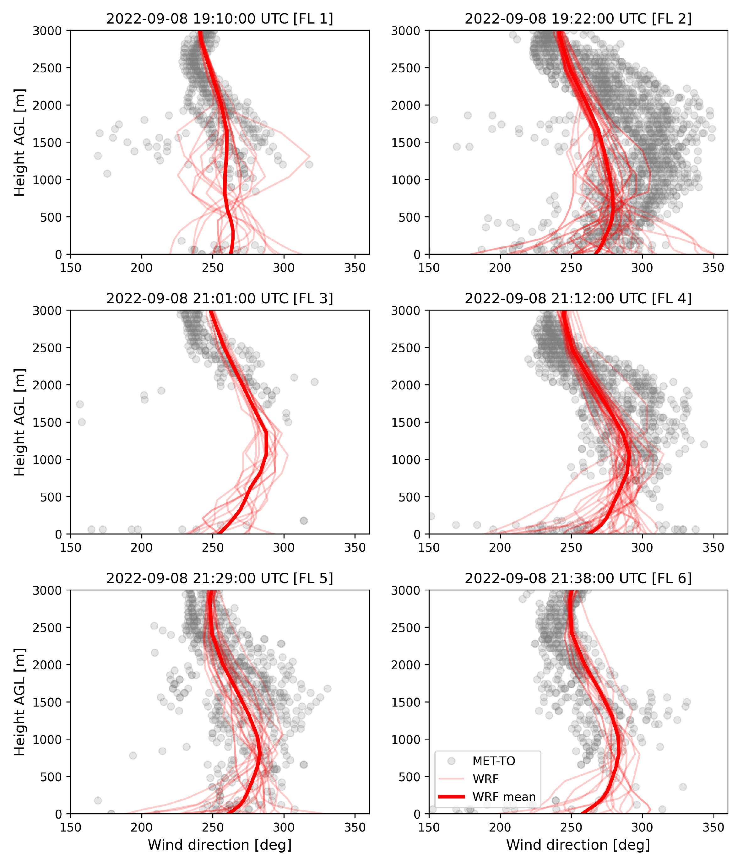
Unlike the surface wind speed, the model simulated wind profiles match closely with the wind profiles observed by MET-TO, especially the WRF model was able to capture the variations in the wind speed magnitude and wind direction profiles (Figure 6 and Figure 7). Capturing these variations is critical for proper plume dispersion above the boundary-layer as it is sensitive to the local shear and/or wind direction shear. The boundary layer height diagnosed from the wind speed profiles from flight legs (FL) 4 and 6, which is around 1300 m, matches closely with the boundary layer height estimated from the backscatter profiles collected by the MET-TO (not shown).
In summary, with the low bias in 2 m temperature and humidity fields and a good qualitative agreement with the upper-air wind speed and wind direction profiles, the WRF simulated meteorology in D02 domain is considered to be accurate enough for initializing the finer scale WRF domain (D03).

Table 2.
Performance metrics for surface variables at individual ASOS stations shown in Figure 3.
Table 2.
Performance metrics for surface variables at individual ASOS stations shown in Figure 3.
| ASOS Station | MET Variable | MAE | MBE | RMSE | R | n |
|---|---|---|---|---|---|---|
| BLU | T2 | 0.91 | -0.23 | 1.1 | 0.93 | 72 |
| RH2 | 3.10 | 0.44 | 3.80 | 0.56 | 72 | |
| U10 | 1.45 | 1.44 | 1.67 | 0.60 | 61 | |
| UDir10 | 44.1 | 3.03 | 78.6 | 0.56 | 49 | |
| GOO | T2 | 1.29 | -0.21 | 1.56 | 0.94 | 72 |
| RH2 | 3.55 | 1.91 | 4.35 | 0.64 | 72 | |
| U10 | 1.34 | 1.35 | 1.50 | 0.44 | 39 | |
| UDir10 | 29.9 | -1.93 | 42.9 | 0.50 | 60 | |
| ANU | T2 | 1.11 | 0.28 | 1.52 | 0.96 | 72 |
| RH2 | 3.06 | -0.21 | 3.85 | 0.72 | 72 | |
| U10 | 2.23 | 2.23 | 2.19 | 0.43 | 64 | |
| UDir10 | 21.9 | 5.69 | 26.7 | 0.85 | 60 | |
| PVF | T2 | 0.96 | 0.24 | 1.23 | 0.96 | 72 |
| RH2 | 3.93 | 3.32 | 4.68 | 0.73 | 72 | |
| U10 | 1.02 | 0.93 | 1.18 | 0.25 | 69 | |
| UDir10 | 30.5 | 6.58 | 52.2 | 0.85 | 69 |
Table 3.
Performance metrics for surface variables averaged across ASOS stations shown in Figure 3.
Table 3.
Performance metrics for surface variables averaged across ASOS stations shown in Figure 3.
| MET Variable | MAE | MBE | RMSE | R |
|---|---|---|---|---|
| T2 | 1.07 | 0.02 | 1.35 | 0.95 |
| RH2 | 3.41 | 1.36 | 4.17 | 0.66 |
| U10 | 1.46 | 1.43 | 1.63 | 0.43 |
| UDir10 | 31.6 | 3.35 | 50.1 | 0.69 |
Figure 5.
Correlation plot between WRF output and ASOS observed values for surface MET fields. The variable compared is mentioned in the title of the subplot.
Figure 5.
Correlation plot between WRF output and ASOS observed values for surface MET fields. The variable compared is mentioned in the title of the subplot.
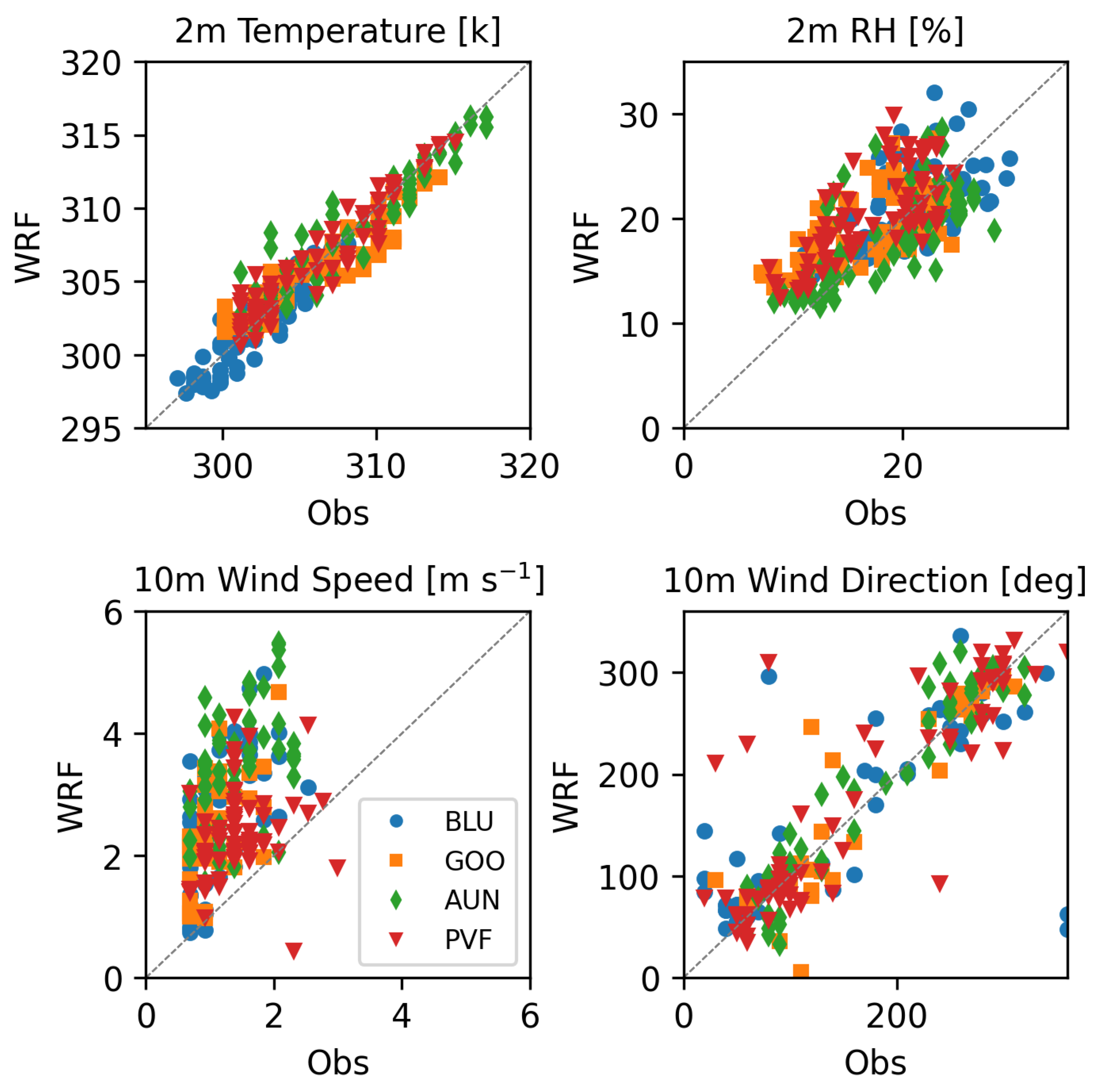
Figure 6.
Wind speed profiles in WRF D02 compared against the MET-TO observations.
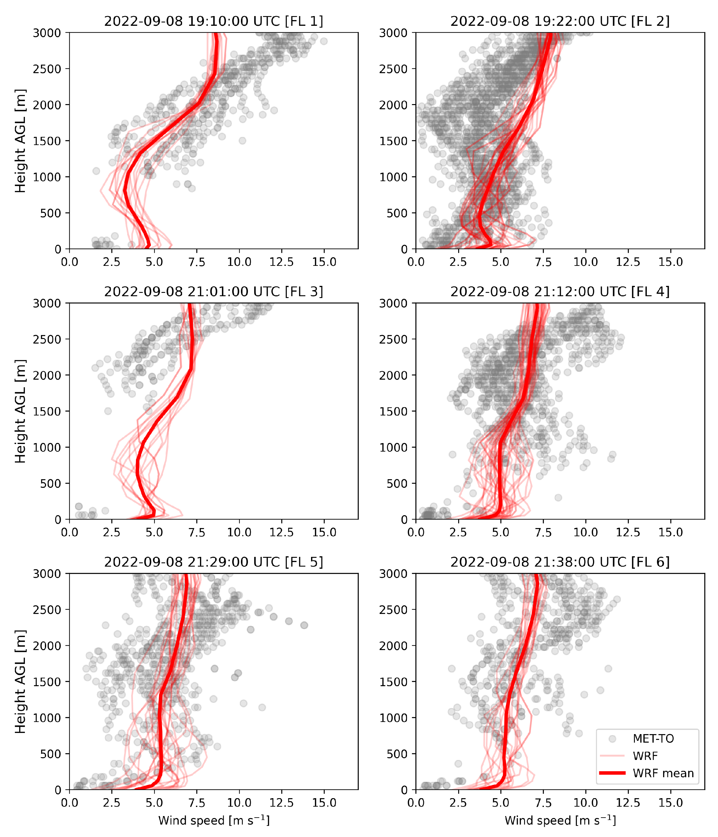
Figure 7.
Wind direction profiles in WRF D02 compared against the MET-TO observations.
3. Analysis of the Atmospheric Boundary Layer
Details of the ABL state from 5pm local time (LT=UTC-7) on 09/08/2022 to 3pm (LT) on 09/09/2022 are given in Table 4. During this period, the depth of the inversion layer varies from 162m to 1502m. The boundary layer is shallow in the late night and early morning hours; it becomes deeper as the day progresses. The stability parameter, , which is the ratio of the depth of the inversion layer to the Monin-Obukhov length, is negative throughout the period, indicating that the atmosphere is in a convectively unstable state, varying from weakly convective in the late night and early morning to highly convective in the mid-to-late afternoon. The shear velocity is imposed by regional meteorology, and varies between 0.22-0.56 m/s. Higher shear velocity is evident between 5am-3pm (LT). During this period, the Monin-Obukhov length is deeper compared to other times, suggesting that wind shear plays an important role in the horizontal transport of the plume closer to the ground. There is a sudden shift in the convective velocity during the morning hours of 09/09. The values vary between 1.0-1.48 m/s from 5 am - 3 pm, 09/09. As expected, higher convective velocities are evident during the afternoon-late evenings. The regimes of the ABL are classified using shear-buoyancy ratio and the atmospheric stability parameter () [21]. The ABL is in a purely convective state and it is highly unstable with large buoyancy-driven vertical mixing when and . In a shear-buoyancy regime, both the shear- and buoyancy forcings are dominant, and during this regime and . The Near-Neutral (NN) ABL regime is shear dominated and is weakly unstable with , .
Turbulence is generated within the ABL due the buoyancy- and shear- forcings from the combined contributions of the heat exchange between the atmosphere and the Earth’s surface and the interaction of the wind with Earth’s surface. The production of turbulence kinetic energy from the wind shear at the surface and at the inversion layer positively contributes to TKE production; meanwhile, production of turbulence kinetic energy from the mean temperature gradient or heat flux at the surface contribute positively during unstable ABL regimes and negatively during stable regimes. The corresponding length scale that represents the relative contributions of shear and buoyancy to the production of TKE is the Monin-Obukhov length (L), which is the ratio of the shear to buoyancy production of TKE, where , is the Von Karman’s constant, and is the mean potential temperature. The value of L is negative throughout the period,indicating convective stability conditions obtain even during the late night and early morning hours of the day. This is expected during the summer in California. The velocity scale for shear-driven processes is the friction velocity (based on the surface shear stress), and for the buoyancy-generating processes is the convective velocity for the buoyancy generated processes (based on the surface heat flux ). ABL regimes are classified depending on the wind speeds and the value of L relative to the ABL depth ().
The buoyancy aspects of ABL behavior follow the cycle of solar heating. However, the regional wind is considerably higher during the afternoon of 09/09 than on the evening of 09/08, which creates differences in the relative importance of buoyancy and wind shear. Specifically, the ABL is in a purely convective regime between 5pm-7pm on 09/08. The ABL is in shear-buoyancy regime from 5am-3pm on 09/09. Accordingly, the ABL transitions between the pure convective and shear- buoyancy regimes during the period of analysis. The evolution of the ABL to a shear-buoyancy regime during the fire has an important effect on the horizontal transport scales of the fire plume.
The statistical averages were calculated from the topographical surface (which is defined as the zero elevation). The terrain is extremely inhomogenous; the topography varies from 400m- 1600m within the numerical domain (see Figure 2). The hourly-averaged mean horizontal and vertical wind speed during the early hours of 09/09 are presented in Figure 8a and Figure 8b, respectively. The hourly averaged mean horizontal wind speeds and temperatures during daytime on 09/09 are presented in Figure 8c and 8d, respectively. During the early morning hours (between 1am-5am), the mean speed exhibits jet-like behavior close to the surface, as seen in both the mean horizontal and vertical velocity profiles. (Early morning horizontal wind-speed detail is provided in Figure 8e.) Daytime warming from 9 am onwards produces a negative temperature gradient close to the surface; convective conditions develop in the ABL, and vertical shear increases in this layer. The peak daytime horizontal wind speed within the ABL is close to 5 m/s. The surface temperature reaches 317 K due to solar heating, and by mid-afternoon (3 pm), a well-developed mixed layer has been produced. In the inversion layer, at 3-4 km above the surface, the regionally imposed horizontal wind peaks in a jet-like structure. Positive shear is produced at the bottom of the jet and negative shear at the top. The maximum wind speed is about 9 m/s in the jet by 3 pm on 09/09 (Figure 8c). Above the inversion layer, the wind speed first decreases and then increases, approaching geostrophic conditions in the free troposphere. As noted earlier, there is a jet-like flow close to the surface between 1am-5am on 09/09.
Table 4.
: Characteristics of the Atmospheric boundary layer between 5 pm 09/08 and 3pm 09/09. Hourly averaged statistics for inversion height (m), Monin-Obukhov’s length L (m), atmospheric stability parameter , friction velocity (m/s), convection velocity (m/s)
Table 4.
: Characteristics of the Atmospheric boundary layer between 5 pm 09/08 and 3pm 09/09. Hourly averaged statistics for inversion height (m), Monin-Obukhov’s length L (m), atmospheric stability parameter , friction velocity (m/s), convection velocity (m/s)
| Time | (m) | L(m) | (m/s) | ||
|---|---|---|---|---|---|
| 5 pm 09/08 | 1502 | -17 | -88. | 0.22 | 1.18 |
| 7 pm 09/08 | 1502 | -22 | -68.3 | 0.24 | 1.18 |
| 9pm 09/08 | 528 | -41 | -12.8 | 0.29 | 1.08 |
| 11 pm 09/08 | 379 | -64 | -5.9 | 0.34 | 1.07 |
| 1am 09/09 | 162 | -68 | -2.4 | 0.34 | 0.88 |
| 3 am 09/09 | 162 | -71 | -2.3 | 0.35 | 0.89 |
| 5 am 09/09 | 258 | -107 | -2.41 | 0.4 | 1.08 |
| 7 am 09/09 | 379 | -183 | -2 | 0.48 | 1.01 |
| 9am 09/09 | 711 | -201 | -3.5 | 0.41 | 1.29 |
| 11 am 09/09 | 932 | -272 | -3.4 | 0.4 | 1.47 |
| 1 pm 09/09 | 1195 | -281 | -4.2 | 0.56 | 1.49 |
| 3 pm 09/09 | 1502 | -105 | -14.3 | 0.4 | 1.48 |
During this time, there is an increase in near-surface vertical velocity. One possible explanation is the formation of nocturnal low-level jets which generally occur at this height. The coastal low-level jet’s in California have been linked to a baroclinic mechanism, in which winds remain in geostrophic balance and a wind speed maximum forms due to the coupling of the thermal wind with a surface layer below. Topography and terrain have been shown to contribute to California coastal jets through the shape of the coastline and to be the dominant factor in barrier jets that form along mountain ranges, such as the Sierra Nevada [40]. Though a jet-like trend is evident in the early morning hours in both the horizontal and vertical wind speed components, the magnitude of the jet is not as high as generally observed with low-level-jets (LLJs) during this season, which is of the order of . In the next section, we investigate whether this is due to domain averaging and the effect of the topography on the wind speed variation.
As noted in Figure 8, there is a jet-like behavior in the wind-speed profile close to the surface. In Figure 9, the wind speed in the plane is plotted, to highlight the influence of topography on the wind speed spatial variation. At 5pm on 09/09, the wind is relatively constant within the entire domain as seen in Figure 9a. Figure 9b-9d shows the wind speed at 1am, 3am and 5 am on 09/09, respectively. During the early morning hours, topography plays a strong role in creating significant gradients across the terrain. Jet-like behavior dominates on Western side of the domain. The effects of topography and the jet-like behavior generate turbulence mechanically during the night. As the sign of the temperature gradient reverses, the turbulence due to buoyancy takes over and topographic effects are not as dominant. This is also expected, as many studies indicate strong topographic effects during the stable conditions([49]).
Contour plots of the hourly averaged vertical velocity fields in the plane are shown in Figure 10. At 5pm on 09/08 (Figure 10a), intermittent (in space) strong shear layer uplift is identified close to the surface. This structure strengthens between 5 pm and 11pm as begins to increase (Figure 10a-10d). The flow field is dominated by strong up and down-drafts that extend to 6km above the surface (Figure 10b-10d). During these times, the ABL is strongly convective, with vertical shear instabilities dominating the transport processes. A clear pattern of alternating updrafts and downdrafts is formed from 5am -onwards. Starting at 5am on 09/09 (Figure 10g-l), well-defined updrafts and downdrafts are evident close to the surface. They extend up to a height of 2km above the surface. To explain this, the domain-averaged horizontal- and vertical- wind profiles in the early morning hours are plotted in Figure 8c and 8d, respectively, are analyzed. At 7 pm on 09/08 the vertical wind shear is strong at the inversion layer, and winds are gentle near the surface. Over the late-night and early morning hours of 09/09, the vertical wind shear is weakened near the inversion layer and the horizontal wind strengthens closer to the surface; within a narrow layer near the surface, very strong shear is generated. Close to the surface, as the day progresses, strong vertical gradients ()develop and the strength of the vertical wind shear increases. Very strong structures develop by mid-afternoon (3pm). However, the increased horizontal wind shear on 09/09 (Figure 8) suppresses convection above the ABL.
The horizontal velocity field in the plane at above the surface at 1 pm on 09/09 is shown in Figure 11a. The flow field is characterized by a pattern of high-speed and low-speed elongated streaks. Above this level, the streaks become less organized and the spacing between them increases with height, as might be expected from the discussion of Figure 12. The horizontal velocity in the plane sampled at the middle of the y dimension at 1 pm on 09/09 is shown in Figure 11b. The ABL is in the shear-buoyancy regime, with winds varying between 4 and 6 m/s, indicating strong shear within the boundary layer, to a height of 1.5 km above the surface. The winds are generally even stronger within the inversion layer, which extends up to 5 km. Above 5 km, winds diminish to the top of the inversion layer. It should be noted that horizontal streaks are not evident (at all heights) until the horizontal winds pick up around 5 am on 09/09. (Figure not shown). Overall, the flow structures reveal the presence of three dynamically distinct regions: the ABL which is below the inversion layer, the inversion layer, and the region above the inversion layer. Within the ABL, buoyancy driven turbulent mixing dictates the flow field, which is characterized by alternating strong updrafts and downdrafts that contribute to the vertical transport of momentum, heat, and species. Within the inversion layer, there is a strong shear-layer produced by strong horizontal winds within this layer, and above the inversion layer, the winds are governed by slower geostrophic winds.
The turbulent kinetic energy (TKE) is analyzed next. The hourly averaged TKE in the plane is given in Figure 12. Figure 12a shows the TKE at 5pm on 09/08. Two distinct regions of high TKE are observed: The first is at a height of 2km above the surface, generated primarily be horizontal wind shear at the bottom of the inversion layer (Figure 8). The second region is defined by TKE generated close to the surface, primarily by buoyant convection close to the surface. However, the near-surface TKE magnitude at this time is much lower than that at 2km at this time. As time progresses, the intensity of TKE at 2 km diminishes and the near-surface TKE becomes stronger (Figure 12b-Figure 12f). The region of high TKE on 09/09 extents up to 500m above the surface. By 1 pm, the TKE builds up to a depth of 2 km (Figure 12j). High TKE corresponds to faster mixing and entrainment. The high TKE is due to the turbulence productions from the combined contribution of shear-generated and buoyancy-generated turbulence. Due to the negative temperature gradient, both the shear- and buoyancy-sources of turbulence production are positive and resulting in higher TKE, whereas during the early morning or nighttime conditions, the shear-generated and buoyancy-generated turbulence counteract each other. TKE also contributes to horizontal transport of momentum and heat. In conclusion, the shear within the inversion layer causes the TKE build-up within this layer during the late evening and early morning conditions. As the day progresses, the turbulence within the boundary layer starts to build-up, and the balance between the TKE in the inversion layer and the turbulence production within the boundary layer together dictate the amount of turbulence generated within the layer.
In summary, the characteristics of ABL between 5pm 09/08 and 3pm 09/09 have been analyzed using the WRF-LES simulations. The results demonstrate that the ABL is in a weekly convective regimes from 5pm 09/08 to 3 am 09/09 and later, the ABL transitions to a shear-buoyancy regime. During this period, the ABL height deepens to a maximum height of 1.2km. Around the time when the smoke plume is introduced (noon on 09/09), strong ABL turbulence had developed within the boundary layer due to solar heating, and in addition, the regionally imposed horizontal wind has also increased. During the shear-buoyancy regime (morning/late afternoon), the turbulence consists of strong up- and down-drafts in the vertical-planes, and with a clear pattern of alternating high-speed and low-speed streaks in the horizontal plane. Two distinct regions of high TKE are observed: The first is at the inversion layer, which is at height of 2km above the surface. In this region, the TKE is generated primarily by horizontal wind shear. The second region is in the near-surface region, where the TKE is generated primarily by buoyant convection. The relative strength of the TKE between the inversion layer and the near-surface region is the key factor of importance and it varies at different instants of the diurnal cycle. During the morning/afternoon hours of 09/09, TKE is higher at the near-surface region than at the inversion height. However, on the previous night, between 11 pm and 1 am, a higher TKE is generated at the inversion layer than in the near-surface region. The vertical structure becomes more organized and extends up to 4 km over the entire domain. It is likely that warm air from the inversion layer is being pushed down and cooler air ascends. As the ground cools, the temperature difference between the inversion height and the surface increases. The turbulence is low during this period, and there is not much mixing resulting in elongated structures indicating that warm columns of air are descending. Between 1am-5am, a localized low level jet develops, producing mechanical turbulence close to the surface, and thus enhancing the turbulence during this time. Topographic effects are also significant during this time resulting in apparent spatial inhomogeneity.
4. Plume Characteristics
A heated air plume was released into the ABL from a continuous circular source located at the ground. For the purpose of this study, the diameter of the source was 400m, and the center of the source was placed at ( N, W). The background ABL velocity profile, temperature profile and surface heat flux, were obtained from the ABL simulations initiated at 11am on 09/09. The plume source gas is lighter than the ambient atmosphere and the density difference generates buoyancy. The LES domain is as follows: 4 km × 4 km × 7 km size (i.e., 10D × 10D × 17.5D) along the two cross-stream (horizontal) and axial (vertical) directions, with the source located at the center of the bottom boundary. The computational domain was discretized using a uniform Cartesian grid with 100 × 100 × 700 nodes in the cross-stream and axial directions. Periodic boundary conditions were imposed on the side boundaries, whereas a constant-pressure boundary condition was imposed at the top. At the center of the bottom boundary, where the source was located, a constant plume surface flux was specified. The heat flux boundary condition elsewhere along the bottom surface was fixed at zero for the entirety of simulation. There was no momentum at the source, so the flow originated purely from the buoyancy difference between the source and the ambient air. The source buoyancy flux () was prescribed as . The total simulation time was 50 minutes.
Figure 13 shows the evolution of the plume over time in the plane over 50 minutes. Initially, the plume is similar to a jet; it transports vertically to a height a 2km without significant mixing (Figure 13a-e). Beyond this height, mixing and entrainment are evident and the plume expands radially outwards (Figure 13a-f). Beyond this height, mixing and entrainment are evident and the plume expands radially outwards (Figure 13g). The mixing results in the plume spreading horizontally and turning toward the surface (Figure 13 h). This further intensifies with time, as seen in Figure 13i, as the plume spreads horizontally to a distance of 1.5km. Figure 14 shows the plume transport and spread at different time instants in the plane (vertically averaged). Initially the plume spreads radially 500m away from the source (Figure 14a); subsequently, it extends horizontally close to 1 km downstream (Figure 14b). Further on, it transports in the cross-wind direction as well (Figure 14c-d). The plume behavior is closely related to the ABL characteristics. During plume injection, the ABL depth is around 1km and TKE is concentrated at a height of 2km above the surface (Figure 7j). The vertical velocity consists of updrafts and downdrafts and which carry the momentum and heat flux of the plume (Figure 5j). The vertical rolls extend to a depth of 2km-2.5km above the surface. At plume release, the underlying ABL dynamics influences the vertical transport and the horizontal spread. Further, the evolution of the ABL over time controls the plume dynamics.
Temperature contours in the plane are shown in Figure 15. The interactions between the atmospheric turbulence with the plume turbulence are seen. During the start of the plume, strong convective turbulence with turbulent bursts near the surface is evident (Figure 15 a-b). At a later time, the higher plume temperatures reach a height of 1 km vertically and 500m horizontally (Figure 15 c). Plume mixing and dilution become stronger, altering the local temperature surrounding the plume (Figure 15d).
5. Conclusions
The purpose of the present work is to complement the CALFIDE field campaign efforts by conducting a numerical modeling study to improve our understanding of the role the ambient atmospheric condition plays in smoke plume transport and mixing. In particular, the Mosquito fire was captured by MISR on 09 September, at 12pm local time in California. We demonstrate the influence that the atmospheric boundary layer evolution has on plume development. Using a high-resolution Advanced Research Version of the Weather Research Forecast Model with realistic boundary conditions derived from the HRRR model, the detailed atmospheric conditions in the Sierra Nevada region, California, United States were simulated, both before and during the plume observation period on 09 September, 12 pm local time.
The ABL simulations have been validated using 4 ASOS stations and NOAA-MET Twin otter. With the low bias in 2 m temperature and humidity fields and a good qualitative agreement with the upper-air wind speed and wind direction profiles, the WRF simulated meteorology is considered to be accurate for the plume simulations.
During the smoke-plume analysis period, the ABL transitions from a purely convective to a shear-buoyancy regime, which has an important effect on the horizontal transport scales of the fire plume. The horizontal transport scales of the plume are governed by the wind shear, wind strength, and local atmospheric turbulence. The boundary layer depth, depth of the turbulent structures, and turbulence intensity in this layer influence the plume vertical transport scales.
There is strong vertical and horizontal shear within the ABL, to a depth of 1.5 km above the surface. In this layer, the horizontal winds are strong, varying between 4 m/s and 6 m/s. Above this layer, much stronger winds are present, up to a height of 5km in the inversion layer. MISR reported a similar pattern of horizontal wind shear: winds of 2.8 m/s below 2 km, and stronger winds of 4.7 m/s above ([39]). The MODIS fire radiative power (FRP) reported a high value of 230 W/m2, and the surface heat flux at the plume source in the model is 240 W/m2. MISR data analysis shows that the near-source plume resides at 3km above the surface, whereas 30 km downwind the smoke approaches the surface. In the present simulation study, the plume reaches a height of 3 km, and there is mixing with the atmosphere up to a height of 4 km during the first hour after initial plume injection. Subsequently, after reaching the maximum height, the mixed layer expands along the downstream direction and bends clockwise towards the surface. There are strong downstream winds of 4.5 m/s within 2km and 6.5 m/s between 2km-4km. Hence, when the plume is within 2km-4km, it is rapidly transported horizontally, and as the plume descends to within 2km of the surface, it slows down. In addition, there is high TKE within this region, and the combination of wind and turbulence dictates the extent of horizontal transport. Overall, it is clear that the ABL height, the height of the vertical rolls (updrafts and downdrafts), and the layer of peak TKE at the inversion level, together control the plume height to be 3 km above the surface. The higher wind speed above the boundary layer, and horizontal winds and the high TKE within the boundary layer, influence the horizontal transport of the plume.
Due to computational limitations, the domain for the plume numerical simulation is 5km, and hence the plume can be tracked over a limited distance compared to the MISR observations, which capture a downwind plume extent estimated to represent about eight hours of smoke emissions. The vertical transport and the trends of the horizontal transport are in good qualitative agreement with the near-source MISR results.
Analysis of the temperature fields provide valuable insight on the influence of the plume on the micro-climate. The ABL is characterized by higher temperature closer to the surface. As the high temperature plume interacts with the ambient temperature fields, the mixing and entrainment cause an increase of the ABL temperature and the mean temperature gradients. The mean temperature gradients result in the generation of additional turbulence fluctuations (Chang and Bhaganagar (2023)). The ABL turbulence is altered along the plume trajectory. As the scales of plume transport are an order of a few kilometers, the influence of the plume on the micro-climate is significant.
The current work is offered as a contribution to wildfire smoke-plume analysis, highlighting the importance of understanding the atmospheric boundary layer state in detail for predicting plume horizontal and vertical transport. In particular, it is important to understand the state of the ABL before and during the spread of the plume. Follow-on work will include running the plume simulation for about eight hours, so capture the estimated range of ages of the full plume observed by MISR.
Acknowledgments
The authors thank Alan Brewer, Chemical Science Laboratory, NOAA for helping access and interpret the NOAA-MET Twin Otter flight observations used in this study. Funding for SB was provided by the NOAA cooperative agreement NA220AR4320151 for the Cooperative Institute for Earth System Research and Data Science (CIESRDS). The statements, findings, conclusions, recommendations, and opinions expressed here are those of the authors and do not necessarily reflect the views of NOAA or the US Department of Commerce.
References
- Andrews, Patricia L. 2007. Behaveplus fire modeling system: past, present, and future. In In: Proceedings of 7th Symposium on Fire and Forest Meteorology; 23-25 October 2007, Bar Harbor, Maine. Boston, MA: American Meteorological Society. 13 p.
- Avolio, E, S Federico, MM Miglietta, T Lo Feudo, CR Calidonna, and Anna Maria Sempreviva. Sensitivity analysis of wrf model pbl schemes in simulating boundary-layer variables in southern italy: An experimental campaign. Atmos. Res. 2017, 192, 58–71. [Google Scholar] [CrossRef]
- Banta, Robert M, Christoph J Senff, Allen B White, Michael Trainer, Richard T McNider, Ralph J Valente, Shane D Mayor, Raul J Alvarez, R Michael Hardesty, David Parrish, et al. Daytime buildup and nighttime transport of urban ozone in the boundary layer during a stagnation episode. J. Geophys. Res. Atmos. 2017, 103, 22519–22544. [Google Scholar]
- Barr, Sumner, Thomas G Kyle, William E Clements, and William Sedlacek. Plume dispersion in a nocturnal drainage wind. Atmos. Environ. (1967) 2017, 17, 1423–1429. [Google Scholar]
- Bhaganagar, Kiran and Sudheer R Bhimireddy. 2017. Assessment of the plume dispersion due to chemical attack on april 4, , in syria. Nat. Hazards 2017, 88, 1893–1901. [Google Scholar] [CrossRef]
- Bhaganagar, Kiran and Sudheer R. Bhimireddy. Numerical investigation of starting turbulent buoyant plumes released in neutral atmosphere. Journal of Fluid Mechanics 2017, 900, 32–1. [Google Scholar]
- Bhimireddy, Sudheer R and Kiran Bhaganagar. Performance assessment of dynamic downscaling of wrf to simulate convective conditions during sagebrush phase 1 tracer experiments. Atmosphere 2017, 9, 505. [Google Scholar]
- Bhimireddy, Sudheer R and Kiran Bhaganagar. Short-term passive tracer plume dispersion in convective boundary layer using a high-resolution wrf-arw model. Atmospheric Pollution Research 2017, 9, 901–911. [Google Scholar]
- Bhimireddy, Sudheer R and Kiran Bhaganagar. Implementing a new formulation in wrf-les for buoyant plume simulations: bplume-wrf-les model. Monthly Weather Review 2017, 149, 2299–2319. [Google Scholar]
- Blaylock, Brian K, John D Horel, and Erik T Crosman. Impact of lake breezes on summer ozone concentrations in the salt lake valley. J. Appl. Meteorol. Climatol. 2017, 56, 353–370. [Google Scholar] [CrossRef]
- Bowman, David MJS and Fay H Johnston. Wildfire smoke, fire management, and human health. EcoHealth 2017, 2, 76–80. [Google Scholar]
- Cannon, Susan H and Jerry DeGraff. 2009. The increasing wildfire and post-fire debris-flow threat in western usa, and implications for consequences of climate change. Landslides–disaster risk reduction 2009, 177–190.
- Carroll, Brian, W. Brewer, Edward Strobach, Neil Lareau, Steven Brown, Mario Valero, Adam Kochanski, Craig Clements, Ralph Kahn, Katherine Noyes, Amanda Makowiecki, Maxwell Holloway, Michael Zucker, Kathleen Clough, Jack Drucker, Kristen Zuraski, Jeff Peischl, Brandi Mccarty, Richard Marchbanks, and Tyler Salas. , 01. Measuring coupled fire-atmosphere dynamics: The california fire dynamics experiment (calfide). Bulletin of the American Meteorological Society 2024. [CrossRef]
- Chang, Chen and Bhaganagar. Energetics of buoyancy-generated turbulent flows with active scalar: pure buoyant plume. Journal of Fluid Mechanics 2017, 954, 23–1. [Google Scholar]
- Clarke, Hamish, Jason P Evans, and Andrew J Pitman. Fire weather simulation skill by the weather research and forecasting (wrf) model over south-east australia from 1985 to 2009. International Journal of Wildland Fire 2017, 22, 739–756. [Google Scholar]
- Coen, Janice L, Marques Cameron, John Michalakes, Edward G Patton, Philip J Riggan, and Kara M Yedinak. Wrf-fire: coupled weather–wildland fire modeling with the weather research and forecasting model. Journal of Applied Meteorology and Climatology 2017, 52, 16–38. [Google Scholar]
- Coniglio, Michael C, James Correia Jr, Patrick T Marsh, and Fanyou Kong. Verification of convection-allowing wrf model forecasts of the planetary boundary layer using sounding observations. Weather Forecast. 2017, 28, 842–862. [Google Scholar]
- Couto, Flavio Tiago, Jean-Baptiste Filippi, Roberta Baggio, Cátia Campos, and Rui Salgado. Triggering pyro-convection in a high-resolution coupled fire–atmosphere simulation. Fire 2017, 7, 92. [Google Scholar]
- De Wekker, Stephan FJ, Meinolf Kossmann, Jason C Knievel, Lorenzo Giovannini, Ethan D Gutmann, and Dino Zardi. Meteorological applications benefiting from an improved understanding of atmospheric exchange processes over mountains. Atmosphere 2017, 9, 371. [Google Scholar]
- Di Giuseppe, Francesca, Florian Pappenberger, Fredrik Wetterhall, Blazej Krzeminski, Andrea Camia, Giorgio Libertá, and Jesus San Miguel. The potential predictability of fire danger provided by numerical weather prediction. Journal of Applied Meteorology and Climatology 2017, 55, 2469–2491. [Google Scholar]
- Dosio, Alessandro, Jordi Vilà-Guerau de Arellano, Albert AM Holtslag, and Peter JH Builtjes. Dispersion of a passive tracer in buoyancy-and shear-driven boundary layers. J. Appl. Meteorol. 2017, 42, 1116–1130. [Google Scholar]
- Dudhia, Jimy. Numerical study of convection observed during the winter monsoon experiment using a mesoscale two-dimensional model. J. Atmos. Sci. 2017, 46, 3077–3107. [Google Scholar]
- Ek, MB, KE Mitchell, Y Lin, P Grunmann, E Rogers, G Gayno, V Koren, and JD Tarpley. Implementation of the upgraded noah land-surface model in the ncep operational mesoscale eta model. J. Geophys. Res. 2017, 108, 8851. [Google Scholar]
- Ferrier, Brad S, Yi Jin, Ying Lin, Thomas Black, Eric Rogers, and Geoff DiMego. 2002. Implementation of a new grid-scale cloud and precipitation scheme in the ncep eta model. In Conference on weather analysis and forecasting, Volume 19, pp. 280–283. AMS.
- Hong, Song-You, Yign Noh, and Jimy Dudhia. A new vertical diffusion package with an explicit treatment of entrainment processes. Mon. Weather Rev. 2017, 134, 2318–2341. [Google Scholar]
- Hu, Xiao-Ming, John W Nielsen-Gammon, and Fuqing Zhang. Evaluation of three planetary boundary layer schemes in the wrf model. J. Appl. Meteorol. Climatol. 2017, 49, 1831–1844. [Google Scholar]
- Janjic, ZI. 1996. The surface layer parameterization in the ncep eta model. World Meteorol. Organ.-Publ.-WMO TD 4–16.
- Jiménez, Pedro A, Jimy Dudhia, J Fidel González-Rouco, JP Montávez, Elena García-Bustamante, Jorge Navarro, Jordi Vilà-Guerau de Arellano, and A Muñoz-Roldán. An evaluation of wrf’s ability to reproduce the surface wind over complex terrain based on typical circulation patterns. Journal of Geophysical Research: Atmospheres 2017, 118, 7651–7669. [Google Scholar]
- Kain, John S and J Michael Fritsch. 1993. Convective parameterization for mesoscale models: The kain-fritsch scheme. In The representation of cumulus convection in numerical models, pp. 165–170. Springer.
- Kolaitis, Dionysios I, Christos Pallikarakis, and Maria A Founti. Comparative assessment of wildland fire rate of spread models: effects of wind velocity. Fire 2017, 6, 188. [Google Scholar]
- Kumar, Mukesh, Branko Kosović, Hara P Nayak, William C Porter, James T Randerson, and Tirtha Banerjee. Evaluating the performance of wrf in simulating winds and surface meteorology during a southern california wildfire event. Frontiers in Earth Science 2017, 11, 1305124. [Google Scholar]
- Lareau, Neil P and Craig B Clements. The mean and turbulent properties of a wildfire convective plume. Journal of Applied Meteorology and Climatology 2017, 56, 2289–2299. [Google Scholar] [CrossRef]
- Linn, Rodman, Jon Reisner, Jonah J Colman, and Judith Winterkamp. Studying wildfire behavior using firetec. International journal of wildland fire 2017, 11, 233–246. [Google Scholar]
- Michael, Yaron, Gilad Kozokaro, Steve Brenner, and Itamar M Lensky. Improving wrf-fire wildfire simulation accuracy using sar and time series of satellite-based vegetation indices. Remote Sensing 2017, 14, 2941. [Google Scholar]
- Mlawer, Eli J, Steven J Taubman, Patrick D Brown, Michael J Iacono, and Shepard A Clough. Radiative transfer for inhomogeneous atmospheres: Rrtm, a validated correlated-k model for the longwave. J. Geophys. Res. Atmos. 2017, 102, 16663–16682. [Google Scholar]
- Mölders, Nicole. Suitability of the weather research and forecasting (wrf) model to predict the june 2005 fire weather for interior alaska. Weather and Forecasting 2017, 23, 953–973. [Google Scholar]
- Noh, Ying, WG Cheon, SY Hong, and S Raasch. Improvement of the k-profile model for the planetary boundary layer based on large eddy simulation data. Bound. Layer Meteorol. 2017, 107, 401–427. [Google Scholar]
- Nottrott, Anders, Jan Kleissl, and Ralph Keeling. Modeling passive scalar dispersion in the atmospheric boundary layer with wrf large-eddy simulation. Atmos. Environ. 2017, 82, 172–182. [Google Scholar]
- Noyes, K. and R. Kahn. , 02. Satellite multi-angle observations of wildfire smoke plumes during the calfide field campaign: Aerosol plume heights, particle property evolution, and aging timescales. Journal of Geophysical Research: Atmospheres 2017, 129. [Google Scholar] [CrossRef]
- Parish, Thomas R. Forcing of the summertime low-level jet along the california coast. Journal of Applied Meteorology and Climatology 2017, 39, 2421–2433. [Google Scholar]
- Peace, Mika, Jesse Greenslade, Hua Ye, and Jeffrey D Kepert. Simulations of the waroona fire using the coupled atmosphere–fire model access-fire. Journal of Southern Hemisphere Earth Systems Science 2017, 72, 126–138. [Google Scholar]
- Price, Samuel “Jake” and Matthew J Germino. Modeling of fire spread in sagebrush steppe using farsite: an approach to improving input data and simulation accuracy. Fire Ecology 2017, 18, 23. [Google Scholar]
- Salesky, Scott T, Marcelo Chamecki, and Elie Bou-Zeid. On the nature of the transition between roll and cellular organization in the convective boundary layer. Boundary-layer meteorology 2017, 163, 41–68. [Google Scholar] [CrossRef]
- S. G. Benjamin, S.S. Weygandt, J.M. Brown M. Hu C.R. Alexander T.G. Smirnova J.B. Olson E.P. James D.C. Dowell G.A. Grell H. Lin S.E. Peckham T.L. Smith W.R. Moninger J.S. Kenyon G.S. Manikin. A north american hourly assimilation and model forecast cycle: the rapid refresh. Monthly Weather Review 2017, 144, 1669–1694. [Google Scholar]
- Shamsaei, Kasra, Timothy W Juliano, Matthew Roberts, Hamed Ebrahimian, Branko Kosovic, Neil P Lareau, and Ertugrul Taciroglu. Coupled fire-atmosphere simulation of the 2018 camp fire using wrf-fire. International journal of wildland fire 2017, 32, 195–221. [Google Scholar]
- Skamarock, William C and Joseph B Klemp. A time-split nonhydrostatic atmospheric model for weather research and forecasting applications. J. Comput. Phys. 2017, 227, 3465–3485. [Google Scholar]
- Solbakken, Kine, Yngve Birkelund, and Eirik Mikal Samuelsen. Evaluation of surface wind using wrf in complex terrain: Atmospheric input data and grid spacing. Environmental Modelling & Software 2017, 145, 105182. [Google Scholar]
- Sullivan, Andrew L. Wildland surface fire spread modelling, 1990–2007. 1: Physical and quasi-physical models. International Journal of Wildland Fire 2017, 18, 349–368. [Google Scholar]
- Weil, Jeffrey C, Peter P Sullivan, Edward G Patton, and Chin-Hoh Moeng. Statistical variability of dispersion in the convective boundary layer: Ensembles of simulations and observations. Bound. Layer Meteorol. 2017, 145, 185–210. [Google Scholar]
- Yerramilli, Anjaneyulu, Challa Venkata Srinivas, Hari Prasad Dasari, Francis Tuluri, Loren D White, Julius Baham, John H Young, Robert Hughes, Chuck Patrick, Mark G Hardy, et al. Simulation of atmospheric dispersion of elevated releases from point sources in mississippi gulf coast with different meteorological data. Int. J. Environ. Res. Public Health 2017, 6, 1055–1074. [Google Scholar]
- Yu, Shaocai, Rohit Mathur, Jonathan Pleim, George Pouliot, David Wong, Brian Eder, Kenneth Schere, Rob Gilliam, and S Trivikrama Rao. Comparative evaluation of the impact of wrf-nmm and wrf-arw meteorology on cmaq simulations for o3 and related species during the 2006 texaqs/gomaccs campaign. Atmos. Pollut. Res. 2017, 3, 149–162. [Google Scholar]
- Yver, CE, HD Graven, Donald D Lucas, PJ Cameron-Smith, RF Keeling, and RF Weiss. Evaluating transport in the wrf model along the california coast. Atmos. Chem. Phy. 2017, 13, 1837–1852. [Google Scholar]
Figure 1.
(a) Top figure: Location of the mosquito fire, b Domains (D01, D02, D03) for the WRF-LES simulations.The plume was initialized at N, W. The fire area mapped in (a) represents an 4 km region centered within the 33 km D03 domain in (b).
Figure 1.
(a) Top figure: Location of the mosquito fire, b Domains (D01, D02, D03) for the WRF-LES simulations.The plume was initialized at N, W. The fire area mapped in (a) represents an 4 km region centered within the 33 km D03 domain in (b).
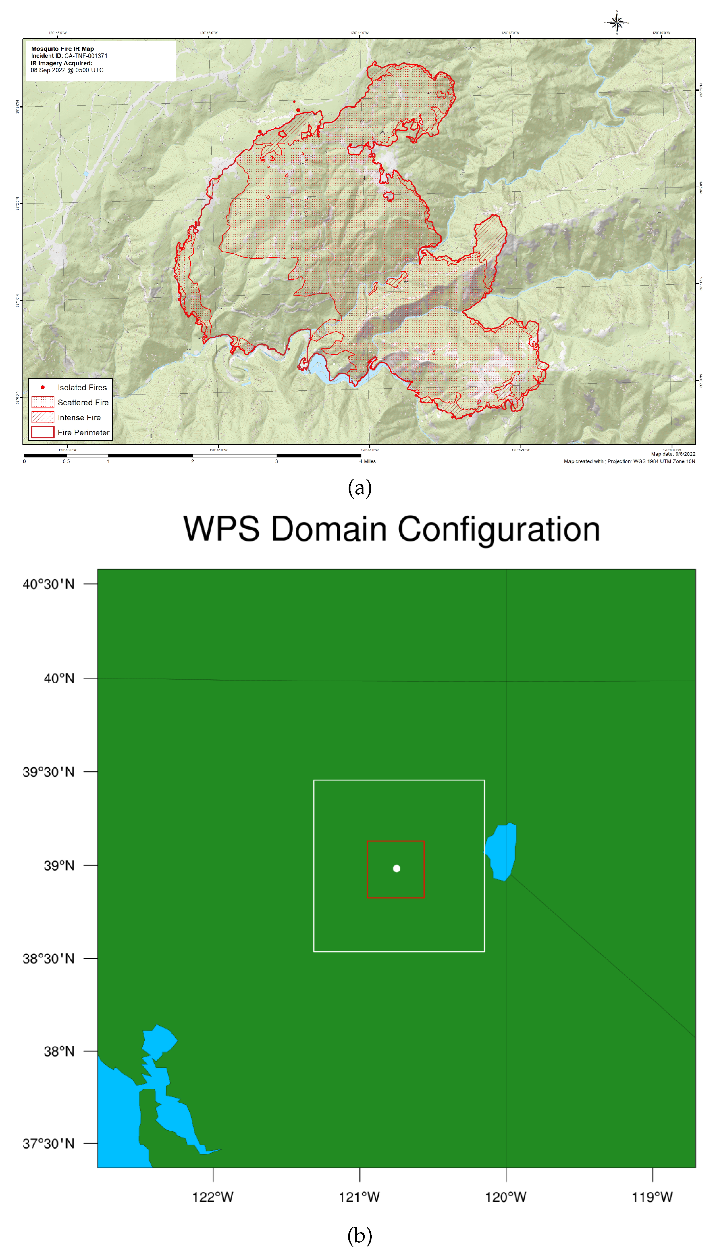
Figure 2.
The boundary conditions obtained from the HRRR initialization data corresponding to the physical domain D03 used in the LES simulation. A. The height of the terrain vs. latitude-longitude, B. The cross-sectional plane of the terrain. The plume was initialized at the center of the region ( N, W)
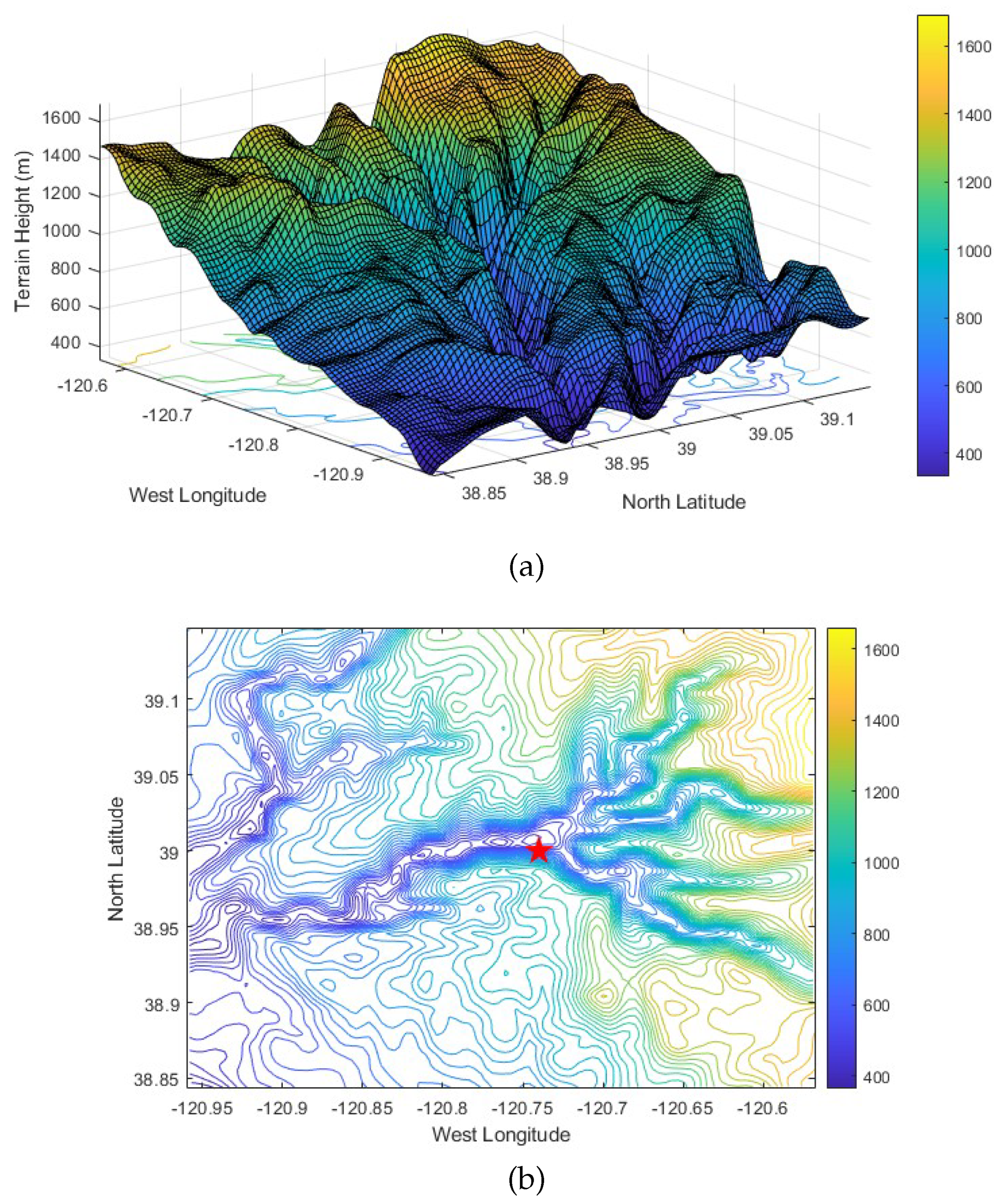
Figure 3.
ASOS station locations in WRF D02.
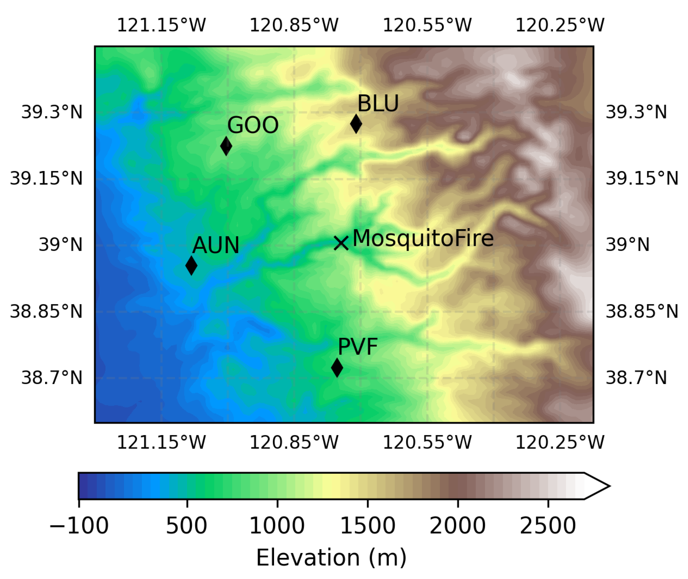
Figure 4.
NOAA-Met Twin Otter flight legs in WRF D02 domain. The value in the paranthesis represents the average flight altitude for the flight leg (FL).
Figure 4.
NOAA-Met Twin Otter flight legs in WRF D02 domain. The value in the paranthesis represents the average flight altitude for the flight leg (FL).
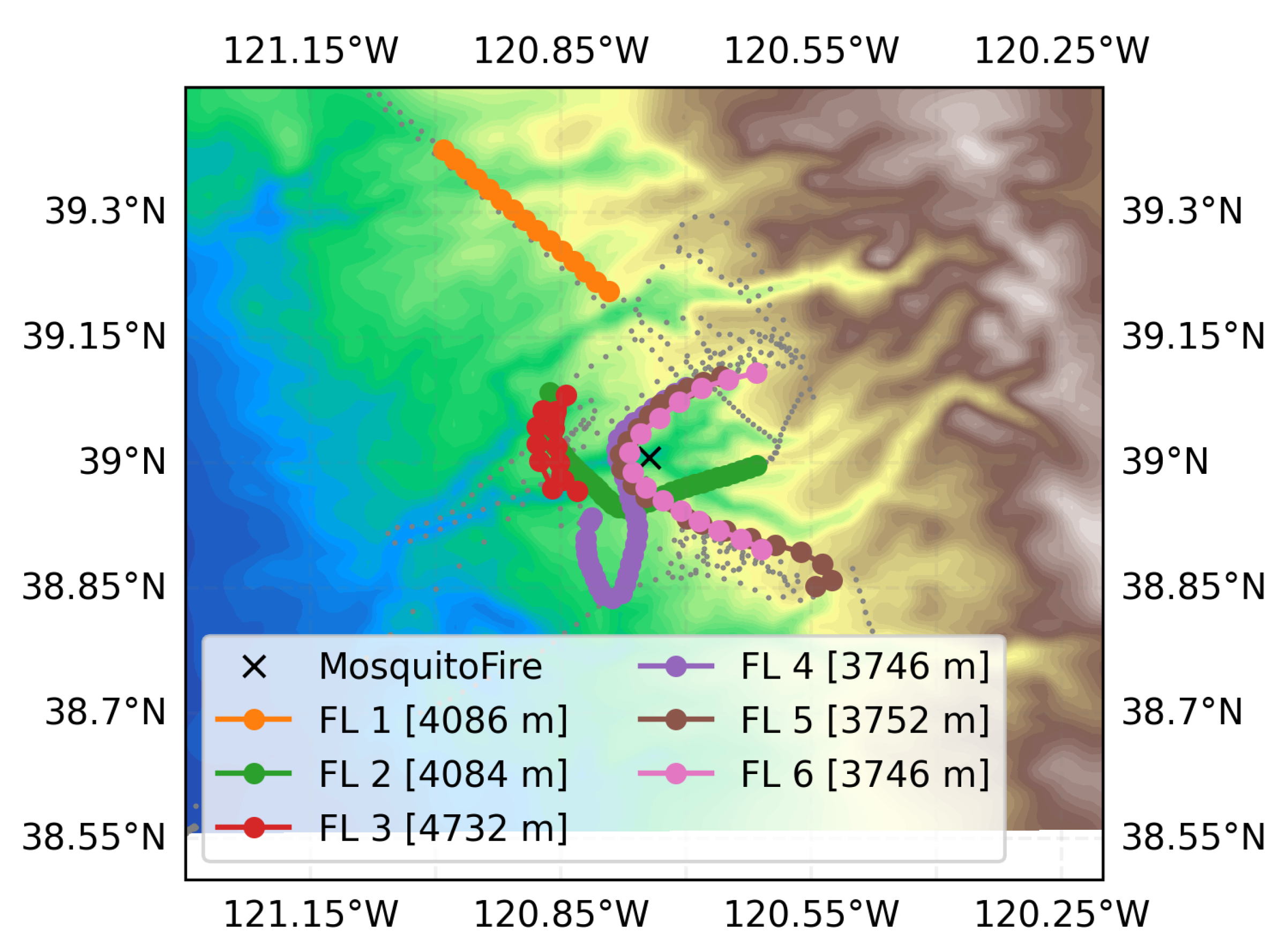
Figure 8.
During the early morning hours of 09/09 the hourly averged profiles of a. horizontal wind speed profiles, b. vertical wind speed profiles, c. mean horizontal wind speed profiles, d. mean temperature profiles.
Figure 8.
During the early morning hours of 09/09 the hourly averged profiles of a. horizontal wind speed profiles, b. vertical wind speed profiles, c. mean horizontal wind speed profiles, d. mean temperature profiles.
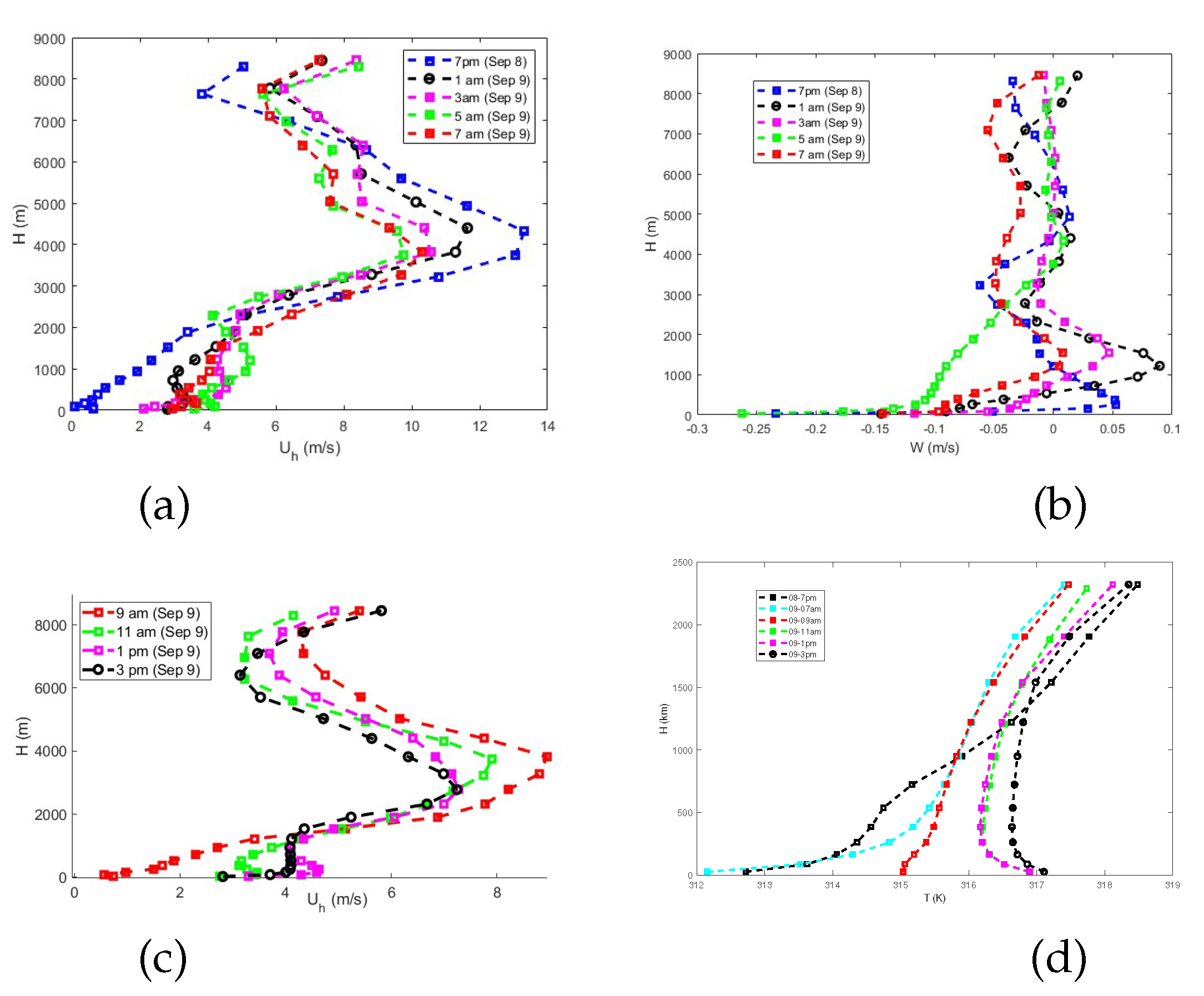
Figure 9.
Contour plot of the wind speed (m/s) plotted in the plane for the D03 domain at a. 5 pm (09/08), b. 1 am (09/09), c. 3 am (09/09), d. 5 am (09/09)
Figure 9.
Contour plot of the wind speed (m/s) plotted in the plane for the D03 domain at a. 5 pm (09/08), b. 1 am (09/09), c. 3 am (09/09), d. 5 am (09/09)
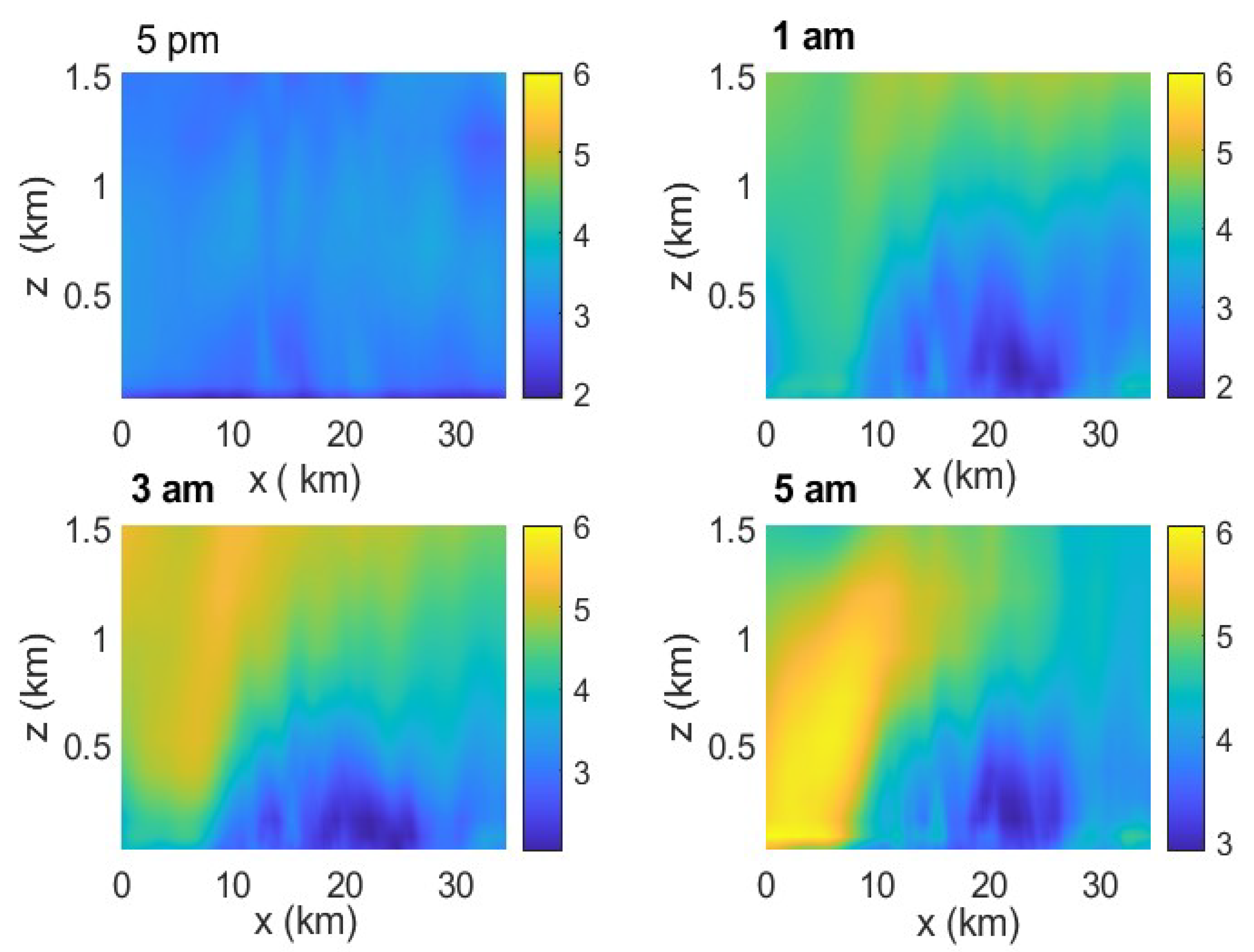
Figure 10.
Contour plot of the vertical velocity in the Mosquito fire plume , sampled in the plane for the D03 domain during 08-09 at a. 5 pm, b. 7 pm, c. 9pm, d. 11 pm, e.1am, f.3am, g. 5am, h, 7am, i. 9am, j. 11am, k. 1pm, l. 3pm. Note the scale changes from panel to panel.
Figure 10.
Contour plot of the vertical velocity in the Mosquito fire plume , sampled in the plane for the D03 domain during 08-09 at a. 5 pm, b. 7 pm, c. 9pm, d. 11 pm, e.1am, f.3am, g. 5am, h, 7am, i. 9am, j. 11am, k. 1pm, l. 3pm. Note the scale changes from panel to panel.
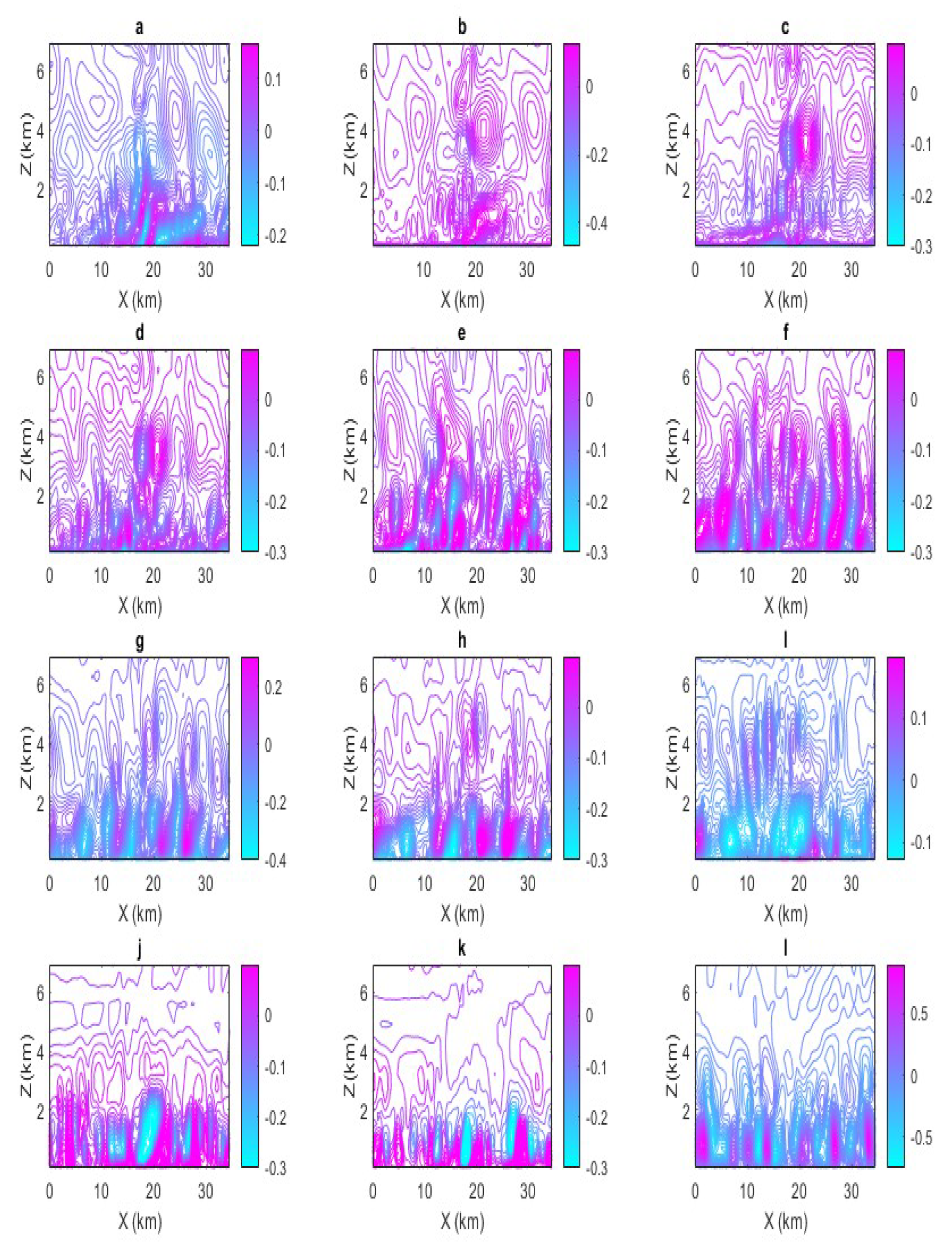
Figure 11.
The contour plot of the horizontal velocity at 1 pm on 09 September a. (top figure) Sampled in the horizontal plane, at above the surface, b. (lower figure) Sampled in plane at the mid-surface.
Figure 11.
The contour plot of the horizontal velocity at 1 pm on 09 September a. (top figure) Sampled in the horizontal plane, at above the surface, b. (lower figure) Sampled in plane at the mid-surface.
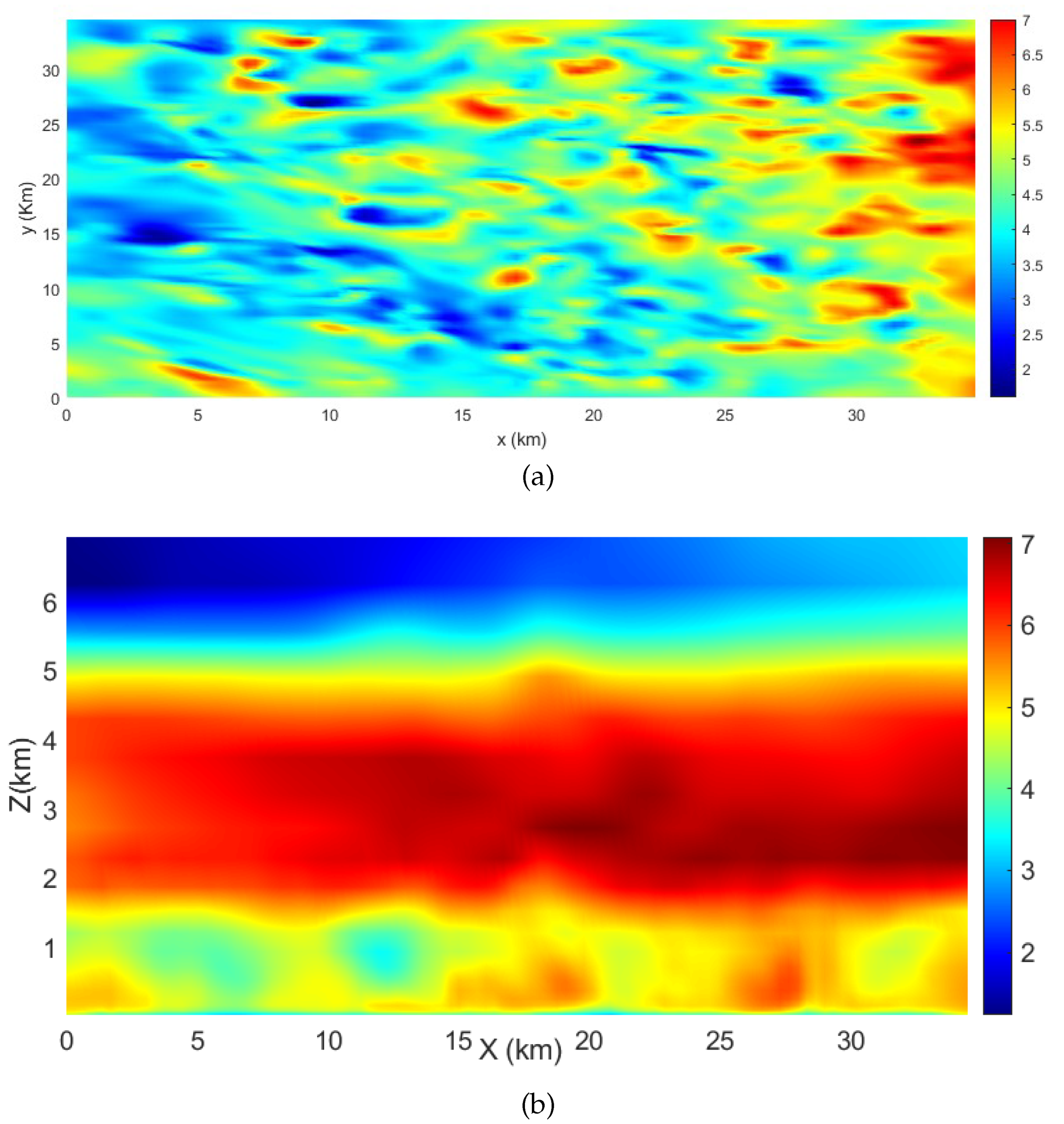
Figure 12.
Contour plot of the Turbulent kinetic energy (TKE) sampled in the plane between 08-09 September plotted at a. 5 pm, b. 7 pm, c. 9pm, d. 11 pm, e.1am, f.3am, g. 5am, h, 7am, i. 9am, j. 11am, k. 1pm, l. 3pm.
Figure 12.
Contour plot of the Turbulent kinetic energy (TKE) sampled in the plane between 08-09 September plotted at a. 5 pm, b. 7 pm, c. 9pm, d. 11 pm, e.1am, f.3am, g. 5am, h, 7am, i. 9am, j. 11am, k. 1pm, l. 3pm.
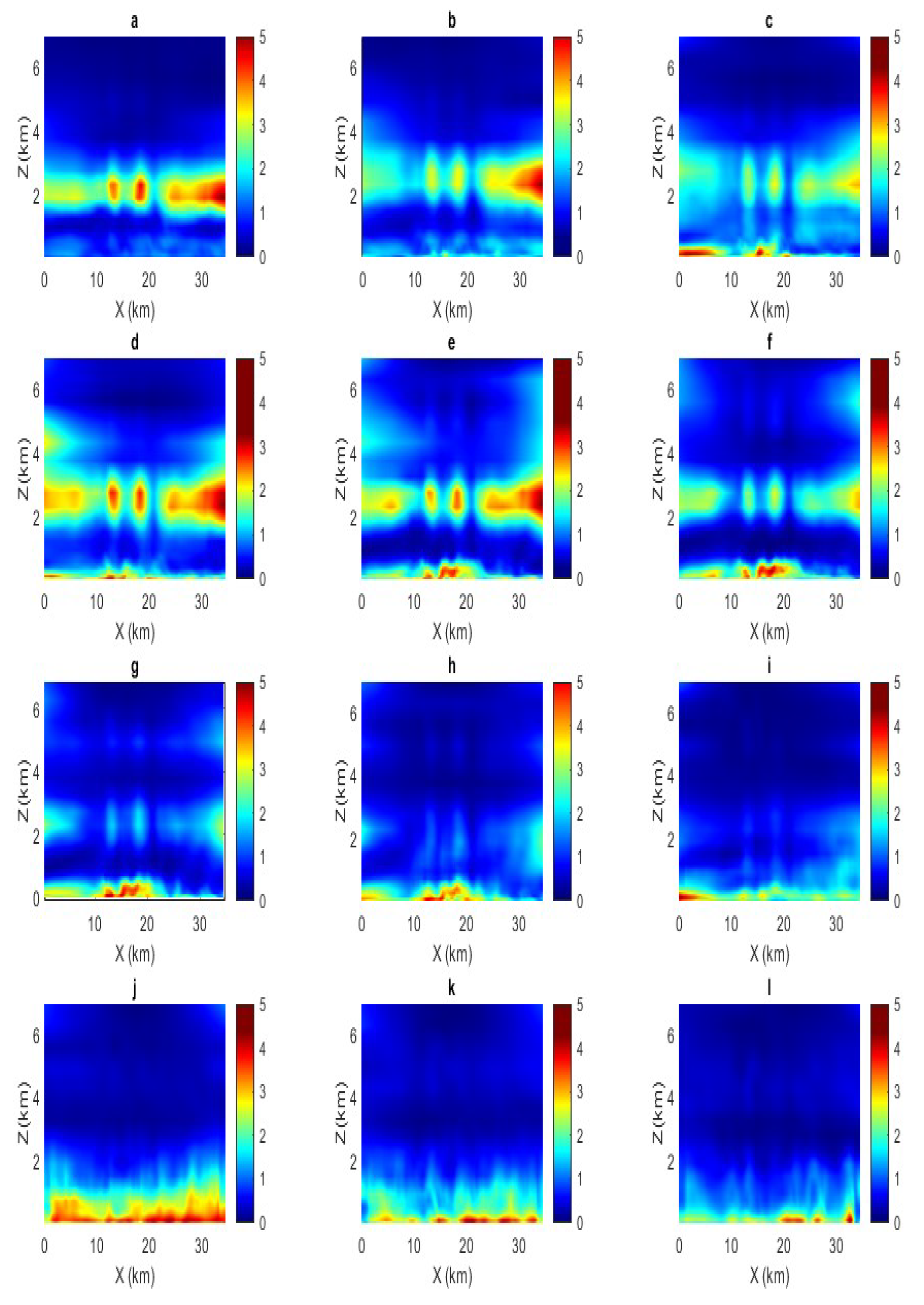
Figure 13.
Contour plot of the plume concentration (kg/kg) sampled in the plane at times from the start of the plume release: a. 10 min, b. 20 min, c. 25 min, d. 30 min, e.40, f.35min, g. 40min, h, 45min, i. 50 min.
Figure 13.
Contour plot of the plume concentration (kg/kg) sampled in the plane at times from the start of the plume release: a. 10 min, b. 20 min, c. 25 min, d. 30 min, e.40, f.35min, g. 40min, h, 45min, i. 50 min.
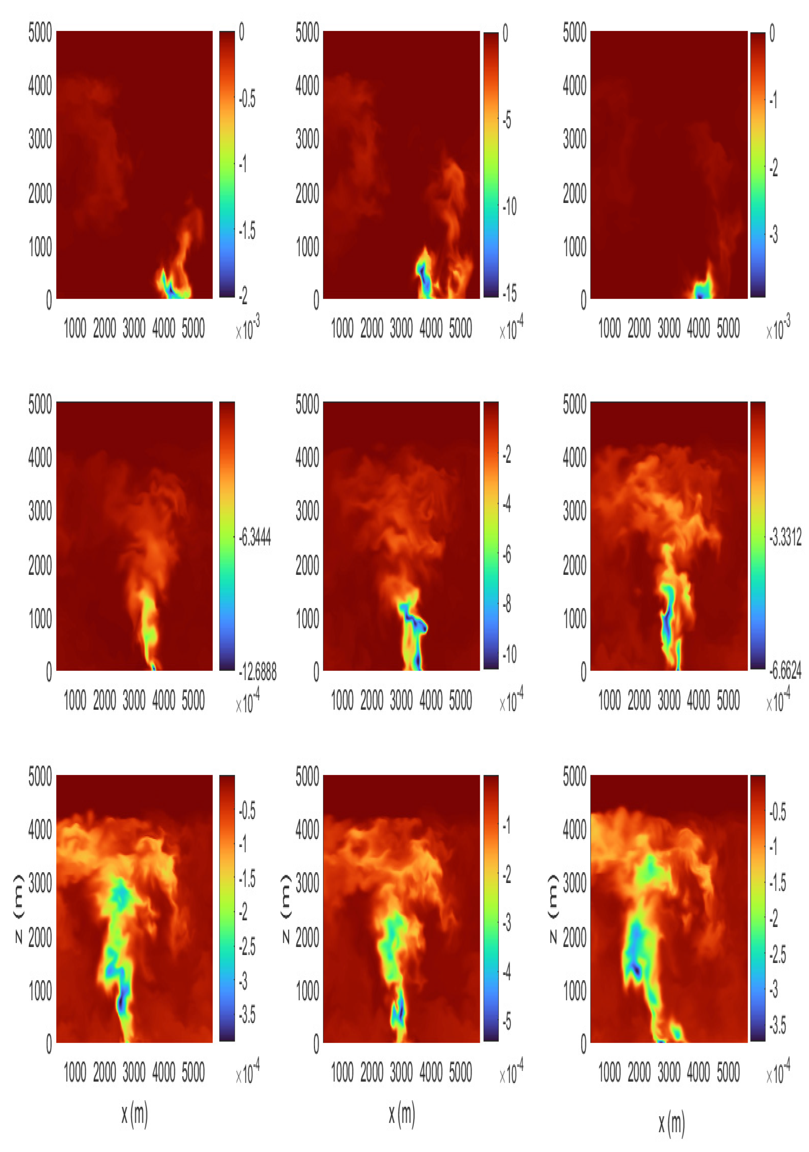
Figure 14.
Contour plot of the plume concentration (kg/kg) sampled in the plane (averaged vertically) at times from the start of the plume release: a. 20 min, b. 30 min, c. 40 min, d. 50 min.
Figure 14.
Contour plot of the plume concentration (kg/kg) sampled in the plane (averaged vertically) at times from the start of the plume release: a. 20 min, b. 30 min, c. 40 min, d. 50 min.
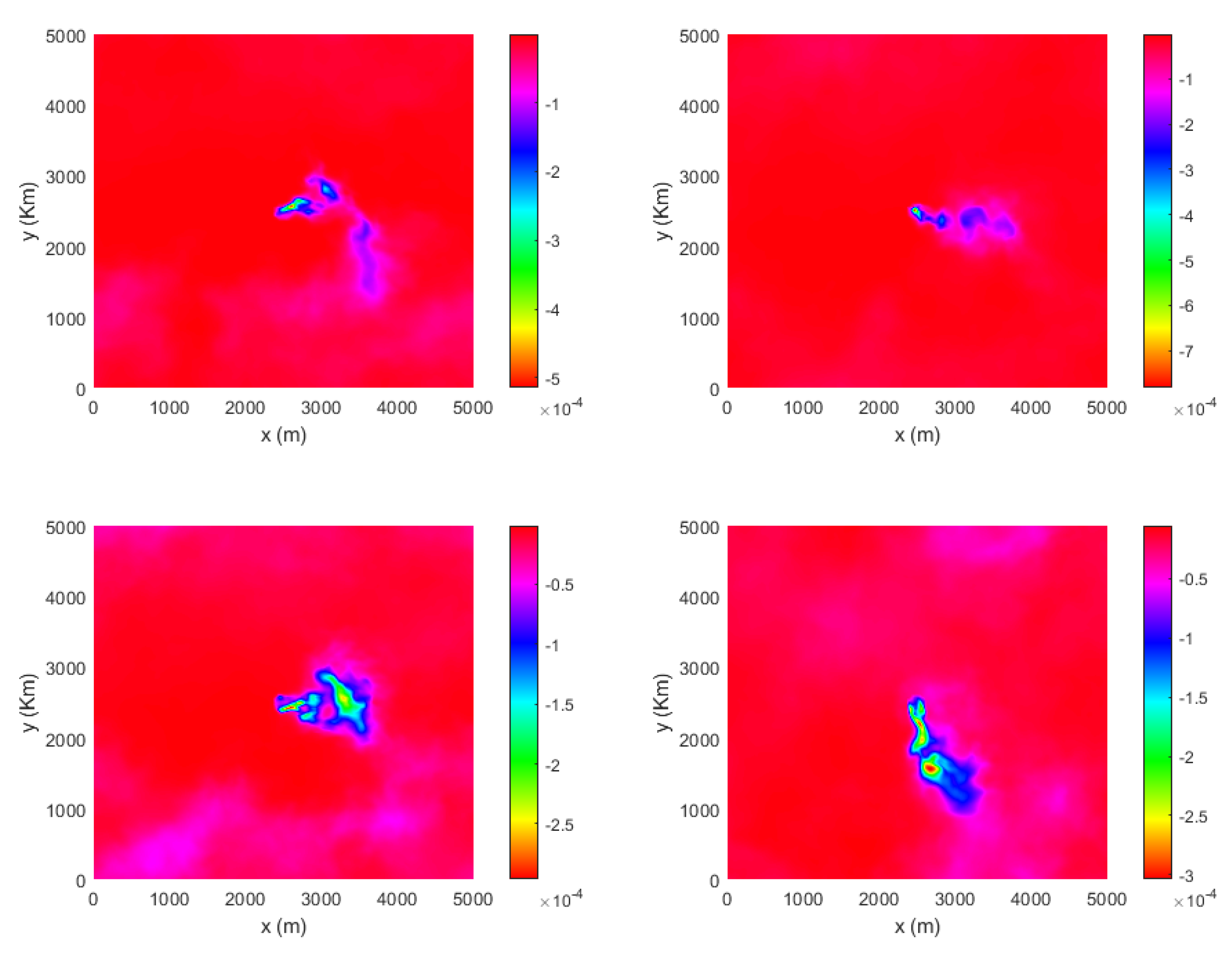
Figure 15.
Contour plot of the plume Temperature field sampled in the plane at times from the start of the plume release: a. 10 min, b. 20 min, c. 30 min, d. 40 min.
Figure 15.
Contour plot of the plume Temperature field sampled in the plane at times from the start of the plume release: a. 10 min, b. 20 min, c. 30 min, d. 40 min.
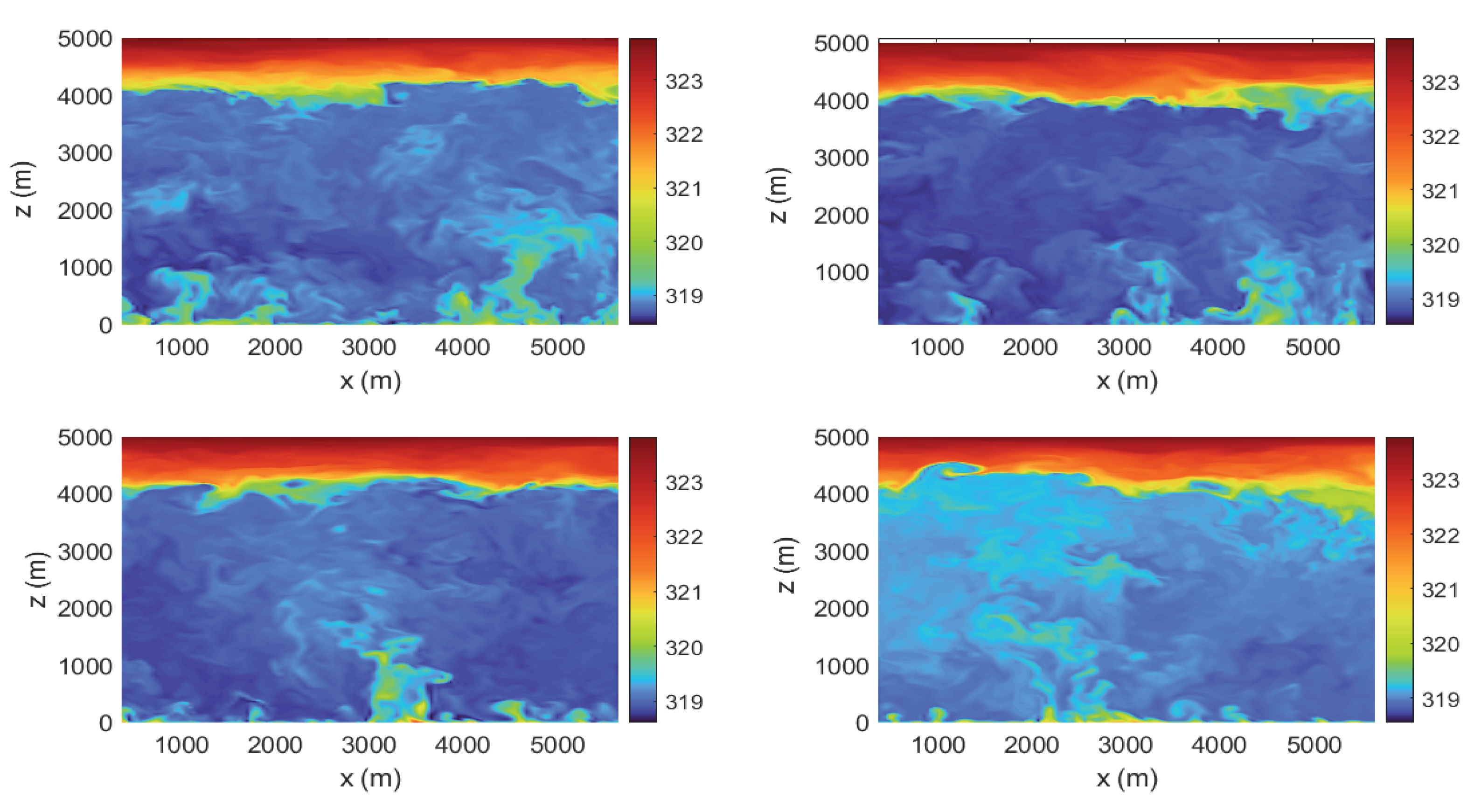
Table 1.
WRF model configuration.
| WRF Model Physics | |
|---|---|
| Longwave Radiation | RRTM scheme [35] |
| Shortwave Radiation | MM5 scheme [22] |
| Microphysics | Ferrier [24] |
| Cumulus | Kain-Fritsch [29] |
| PBL | YSU scheme with ysu_top_downmixing turned "on" [25,26,37] |
| Surface layer | Monin-Obukhov [27] |
| Land Surface model | Noah LSM [23] |
Disclaimer/Publisher’s Note: The statements, opinions and data contained in all publications are solely those of the individual author(s) and contributor(s) and not of MDPI and/or the editor(s). MDPI and/or the editor(s) disclaim responsibility for any injury to people or property resulting from any ideas, methods, instructions or products referred to in the content. |
© 2025 by the authors. Licensee MDPI, Basel, Switzerland. This article is an open access article distributed under the terms and conditions of the Creative Commons Attribution (CC BY) license (http://creativecommons.org/licenses/by/4.0/).
Copyright: This open access article is published under a Creative Commons CC BY 4.0 license, which permit the free download, distribution, and reuse, provided that the author and preprint are cited in any reuse.


