
Submitted:
11 November 2025
Posted:
12 November 2025
You are already at the latest version
Abstract
The first (main) aim of the article is to define and practically apply the parameterized Kolmogorov-Smirnov goodness-of-fit test for normality. These modifications consist in varying a formula for calculating the empirical distribution function (EDF). The second contribution is to expand the EDF family with four new proposals. The third contribution is to create a family of alternative distributions, consisting of both older and newer distributions that, thanks to their flexibility, belong to all groups of skewness and kurtosis signs. Critical values are obtained using 106 order statistics for sample sizes n = 10, 20 and at a significance level a = 0.05. The fourth contribution is to calculate the power of the analyzed tests for alternative distributions based on 105 values of test statistics, with parameters selected so that they are similar to the normal distribution in various ways. The effectiveness of the analyzed tests is illustrated by analyzing real datasets.
Keywords:
goodness-of-fit test
; tests for normality
; kolmogorov-smirnov test
; lilliefors test
; test power
1. Introduction
Numerous goodness-of-fit tests (GoFTs) have been considered and applied in many scientific fields. GoFTs for normality are very popular in economics and finance. GoFTs are used to analyze market behavior (distribution of rates of return, trading volume or asset prices), assess market efficiency and identify deviations from ideal market conditions, analyze stochastic processes (asset prices or changes in commodity prices). In demography, the fertility curve is almost normally distributed. In econometrics, normality tests are used to check whether regression errors are normally distributed. This is important for the proper evaluation of regression models because violating the assumption of normality can lead to erroneous statistical conclusions.
One of the most common normality testing procedures available in statistical software is the Kolmogorov-Smirnov (KS) test [1,2], which belongs to the empirical distribution function (EDF) tests. Other popular EDF tests include the Cramer-von Mises (CM) test [3,4], Lilliefors (LF) test [5], Kuiper (K) test [6], Watson (W) test [7] and Anderson-Darling (AD) test [8].
Let be independent, sorted, and identically distributed observations from an unknown continuous cumulative distribution function (CDF) . We wish to determine whether coincides with the cumulative distribution function (CDF) of the normal distribution . Then, we are interested in testing the following hypothesis against . The EDF is given by , where for and for .
The -corrected KS test [9], investigated further by Khamis [10,11,12], redefines the value of the EDF at the data points and compares the redefined EDF to the CDF at the data points. Let the EDF at the i-th data point be given by
Harter [9] selected for study.
Bloom [13] proposed the transformation
to decrease the mean square error (MSE) of certain statistics. Note that . The transformation (2) was used to create the GoFTs.
Sulewski [14] used the Bloom’s formula to create the one-component LF GoFT with statistic
We know perfectly well that the greatest discrepancy between the theoretical and empirical distribution functions may occur at different positions in the series. The probability of this discrepancy occurring for a given positional statistic is smaller the more extreme is. Hence, the idea of a two-component test statistic described in [15]. The first component is, as in the original LF test, absolute value of the greatest discrepancy between sample and population distributions. The second component is a position in an ordered sample at which this discrepancy is located.
Sulewski and Stoltmann [16] used the Bloom’s formula to create the modified CM (MCM) GoFT with statistic
Simulation studies for the MCM test and for the one- and two-component LF tests were carried out for the following methods of calculating :
- – occurs in the KS statistic,
- – occurs in the KS statistic,
- – occurs in the CM statistic,
- – the mean value of i-th order statistics of the beta distribution,
- – the median of i-th order statistics of the beta distribution,
- – the mean value of i-th order statistic of the normal distribution,
- – founded by Filliben [17],
- – founded by Harter [9].
Six of the EDF definitions listed above (except and ) have .
Recently, many articles have been devoted to the goodness-of-fit tests (GoFTs) for normality. Table 1 shows the authors of works created in the 21st century and analyzed sample sizes. Sample sizes are in bold.
The small samples that dominate in Table 1, can be used in experimental economics, where papers were published with samples of a dozen or so people in a group. This is where strong tests can be put to great use. It may happen that the results will be: in the original paper, the hypothesis was accepted, and when a stronger test is applied, the hypothesis is rejected.
The first (main) aim of the article is to define and practically apply the parameterized KS test for normality. The second aim is to expand the EDF family with four new proposals. The third aim is to create a family of alternative distributions (alternatives), consisting of both older and newer distributions that, thanks to their flexibility, belongs to various groups of skewness and excess kurtosis signs. The fourth aim is to calculate the power of the analyzed tests for alternatives based on values of test statistics, with parameters selected so, that alternatives are similar to the Gaussian distribution in various ways.
The rest of this article is structured as follows. In Section 2, we define the parameterized KS GoFT test for normality. Section 3 is devoted to the similarity measure of the alternative to the normal distribution. In Section 4, we present the alternatives divided into nine groups according to their skewness and excess kurtosis signs (values). Power study is presented in Section 5 and real data examples are provided in Section 6. Finally, concluding remarks are presented in Section 7. Additional material can be found in Appendix.
2. Parameterized Kolmogorov-Smirnov Test for Normality
Before we present the parameterized KS test (the first contribution of the paper), we would like to expand the EDF family (the second contribution of the paper) with four new proposals and given by
thus, eight of the EDF definitions listed earlier are on the line and five of them are on the line (see Figure 1). The previously analyzed values unevenly fill the line on the interval . Four values belong to the interval . The value represents the interval and the values 0.9 represent the interval . The new representatives of line, also located at the corners of the square, are EDFs with and .
Let . Let’s remember that the KS test statistic is given by the formula
Our idea is to parametrize the EDF in (5) using the Bloom’s formula (2). Parametrized KS (PKS) test statistic is defined as
Note that .
3. Similarity Measure
Let’s assume that and , . The Malachov inequality is defined as [57].
A review of recent statistical literature shows that cases with small skewness and excess kurtosis values do not dominate in testing for normality. It is very interesting to see how the GoFTs responds to samples coming from alternatives close to the normal distribution.
Let be a PDF of the alternative distribution with the vector of parameters . The similarity measure M of the alternative distribution (A) to the normal distribution is defined as [14]
where is the PDF of the normal distribution. The takes values on . The when PDFs are identical.
Figure 2 shows values of the similarity measure , when an alternative distribution is the Student t distribution with v degrees of freedom. Note that if then obviously .
4. Alternative Distributions
As mentioned earlier, there are many articles devoted to testing for normality. In these articles, many alternative distributions (alternatives) have been used, among them asymmetric and symmetric ones. Recall that symmetric distributions with undefined and are Cauchy and slash distributions.
The alternatives can be divided into four groups, depending on the support and shape of their densities (see e.g. [49,58]. These groups include symmetric alternatives with support , asymmetric alternatives with support , alternatives with support and alternatives with support . Gan and Koehler [59], Krauczi [60] and Torabi et al. [49] divided alternatives into five groups, namely: asymmetric short-tailed, asymmetric long-tailed, symmetric short-tailed, symmetric close to normal and symmetric long-tailed alternatives. Sulewski [14,15] divided alternatives into twelve groups A1-F2 due to their and signs as well as bimodality.
Our idea is to divide the alternatives into nine groups according to their and signs [16]. Groups 0, A-H are defined in Table 2.
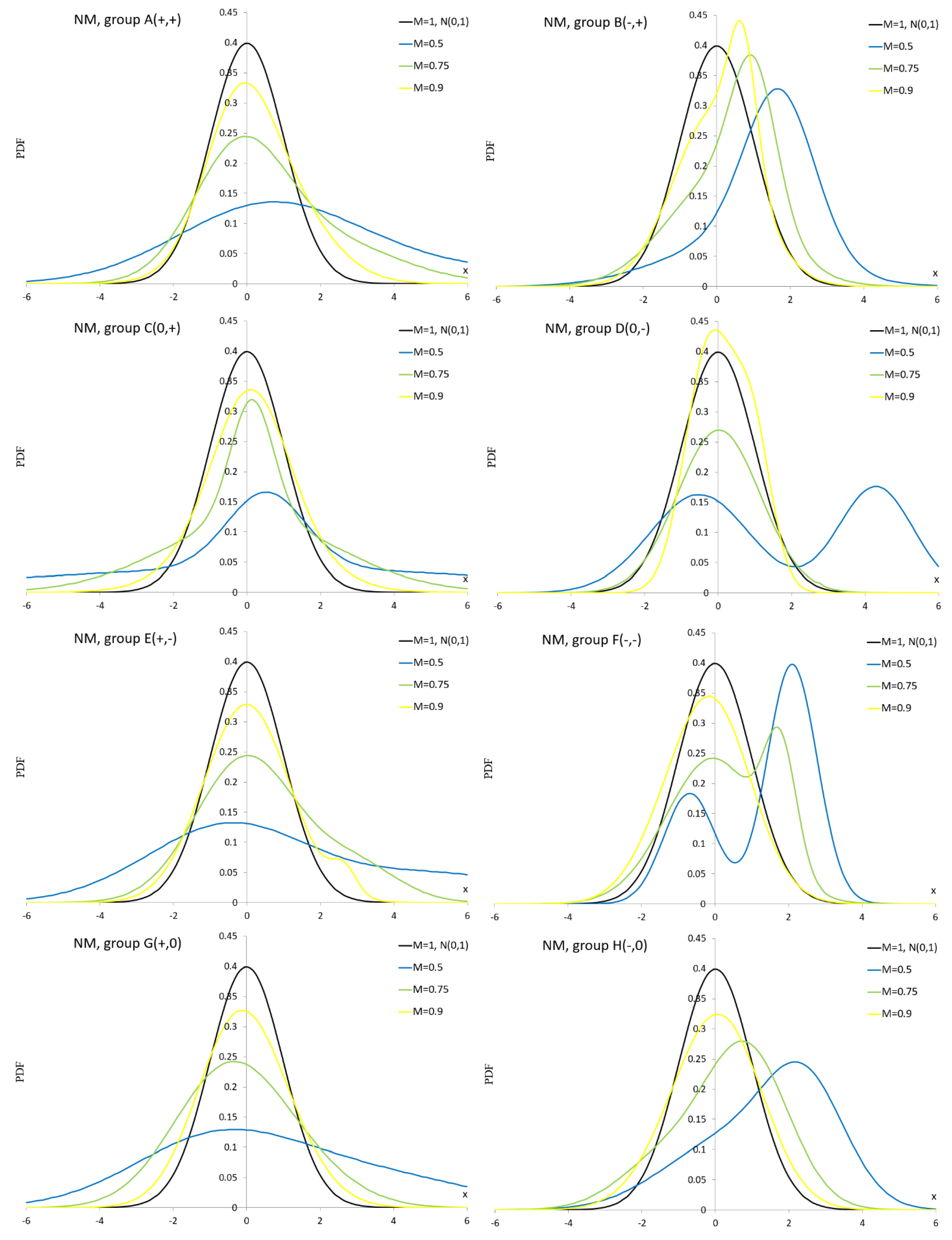
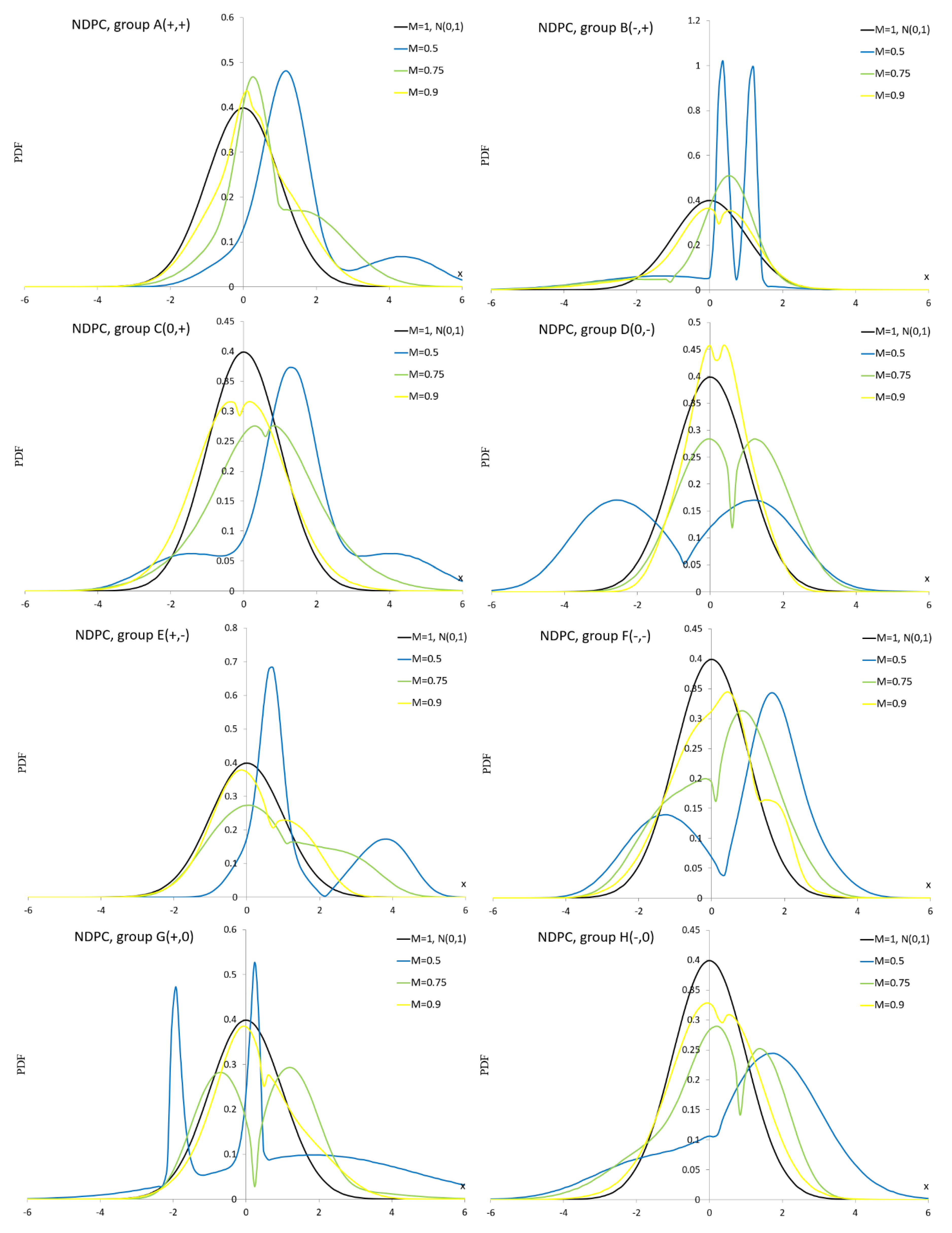
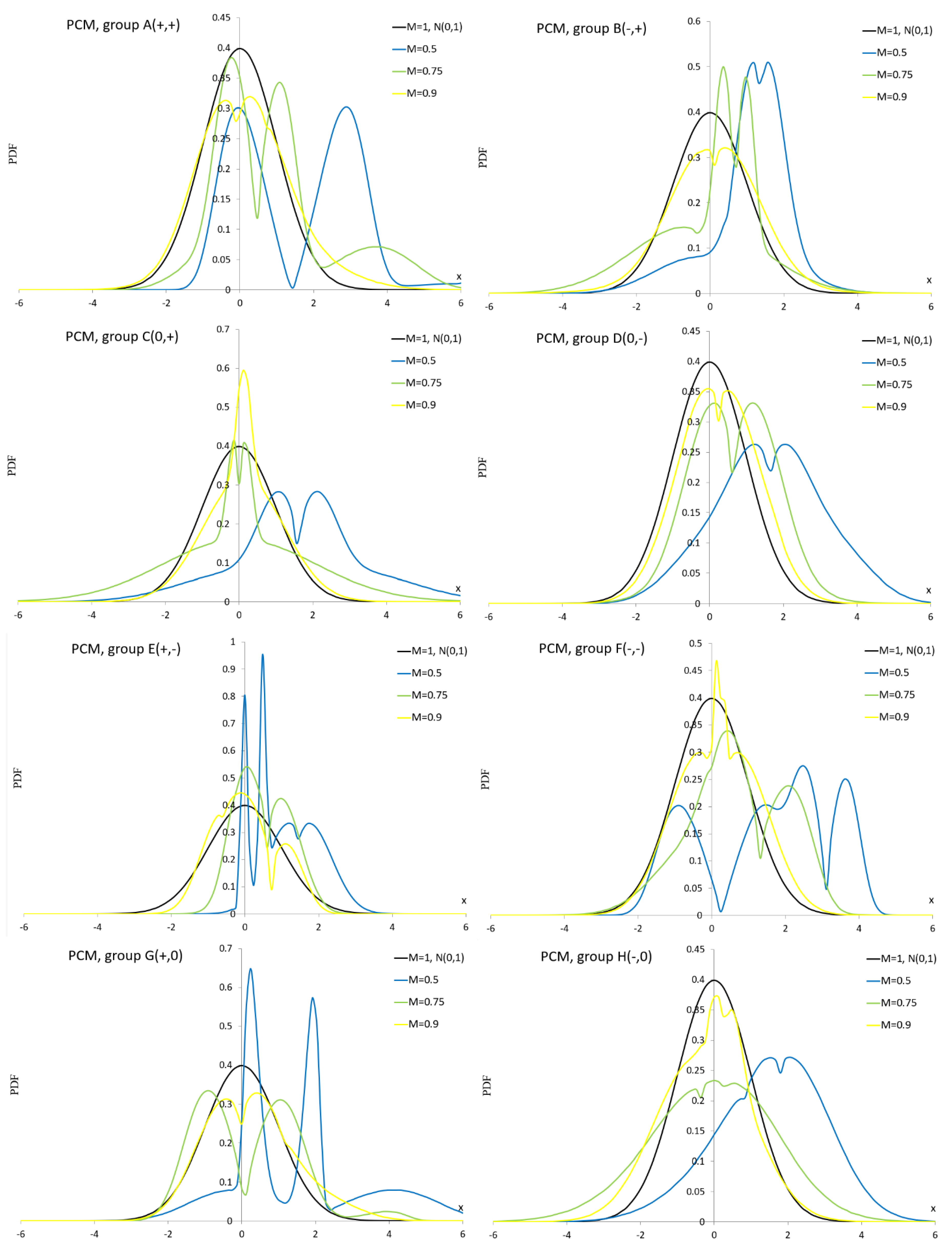
The first (main) criterion for selecting an alternative for Monte Carlo simulation is that and calculated for the alternative parameters belong to all analyzed groups. This criterion is fulfilled by five distributions defined in an infinite domain, such as: the Edgeworth series (ES) and Pearson (P) as monolithic distributions with parameters and , the normal mixture (NM) as a mixture of two normal distributions, the normal distribution with plasticizing component (NDPC) as a mixture of normal and non-normal distributions and the plasticizing component mixture (PCM) as a mixture of two identical non-normal distributions.
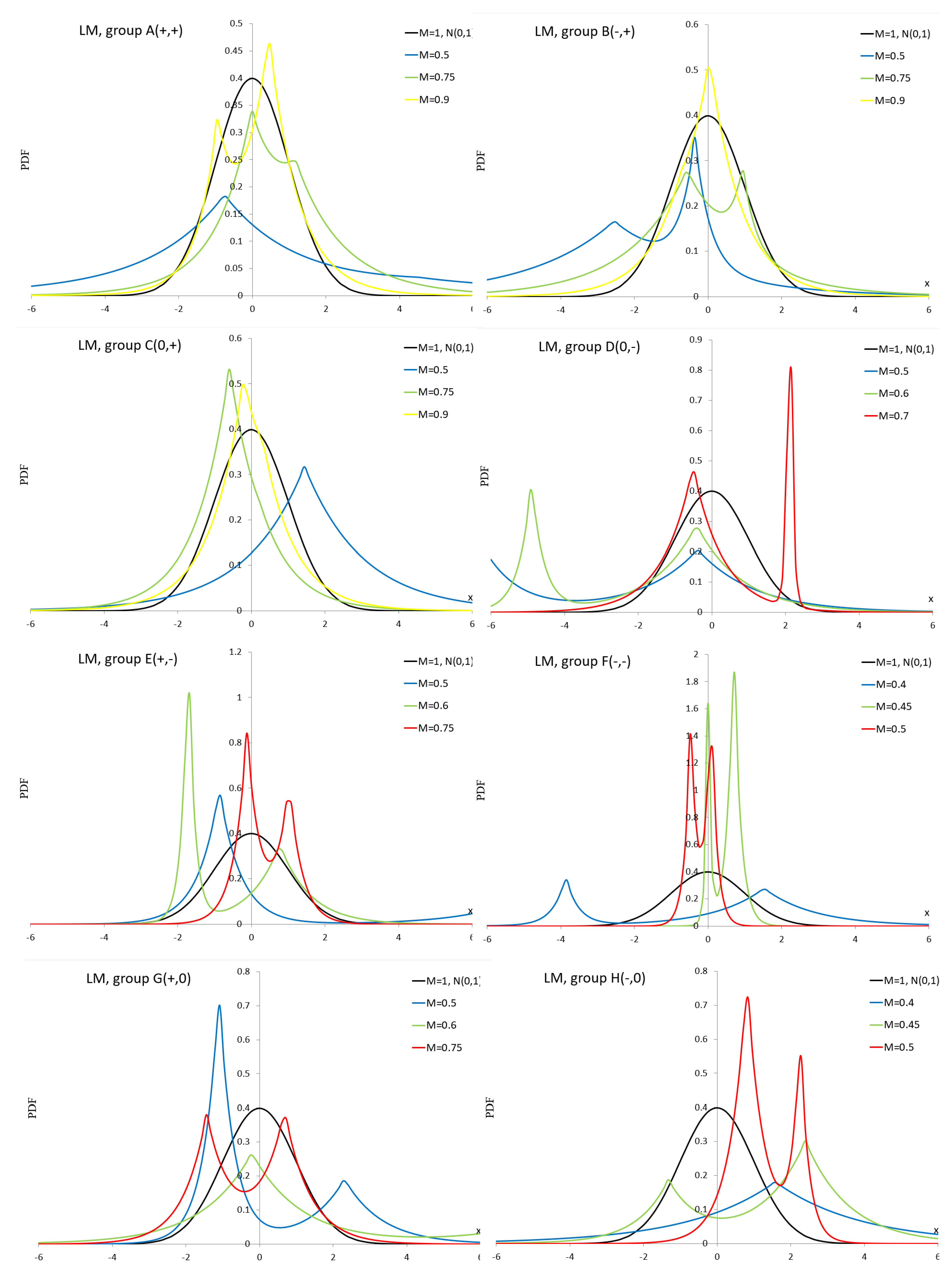
The second criterion for selecting an alternative distribution for Monte Carlo simulation is that and calculated for the alternative parameters belong to all analyzed groups except one (group 0). This criterion is fulfilled by the Laplace mixture (LM) distribution belonging to the groups A – H and defined in an infinite domain.
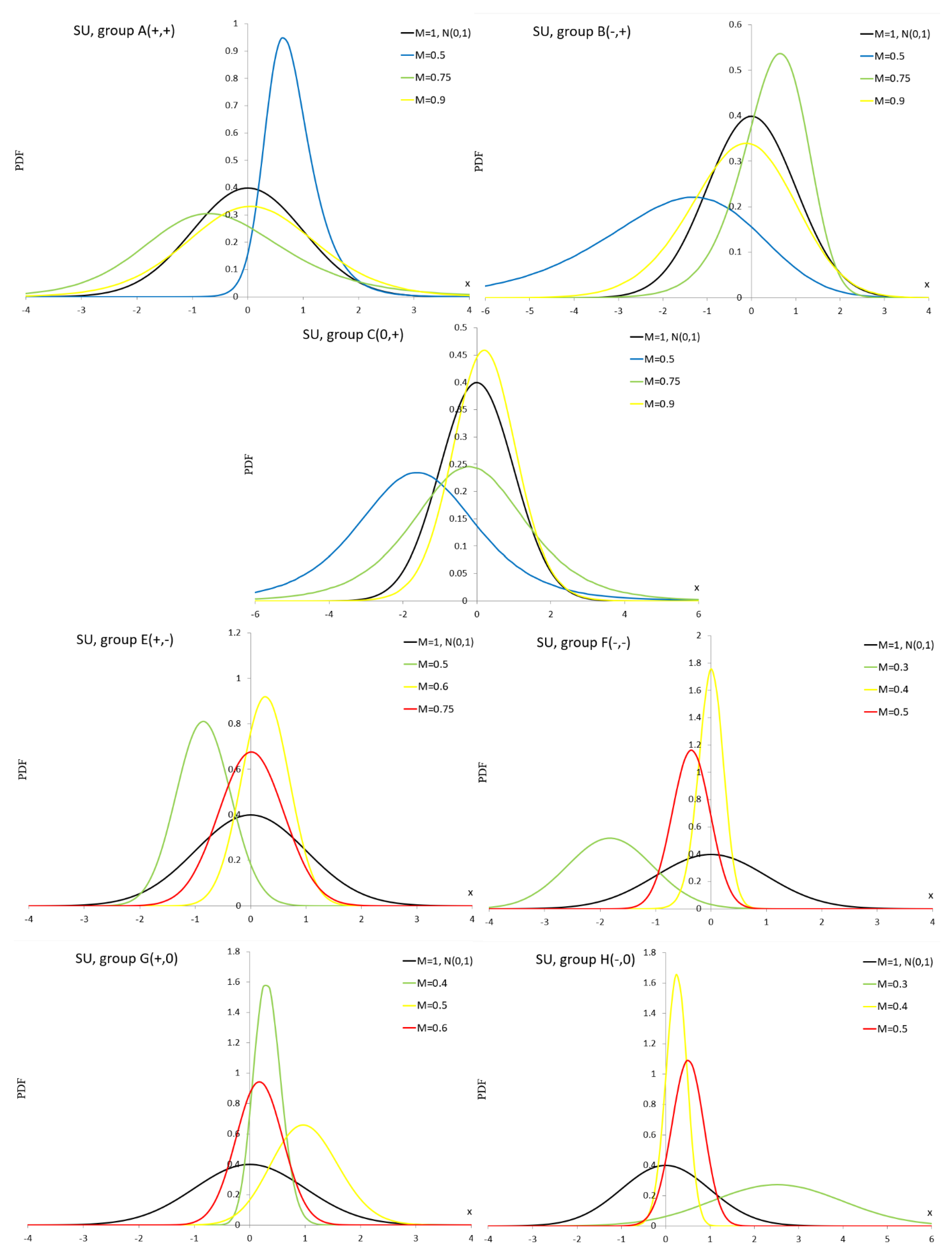
The third criterion for selecting an alternative for Monte Carlo simulation is that and calculated for the alternative parameters belong to all analyzed groups except two groups. These alternatives can be very similar to the normal distribution. This criterion is fulfilled by the SB Johnson distribution (except groups 0, C) and SU Johnson distribution (except groups 0, D).
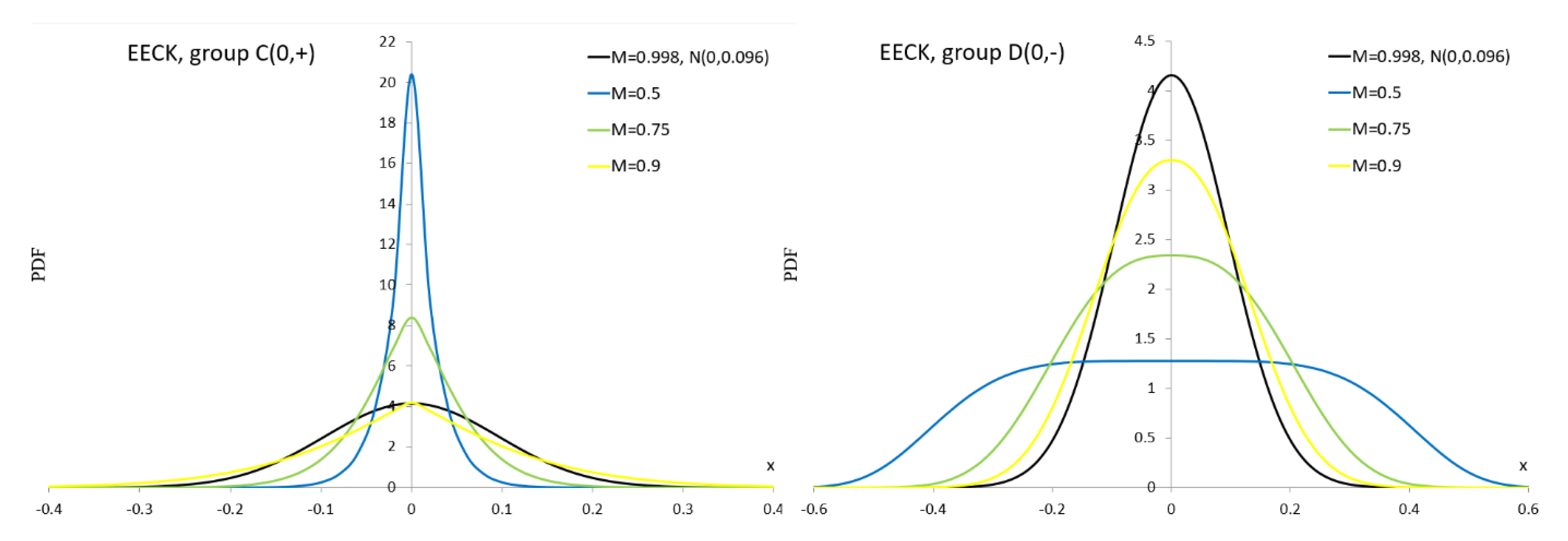
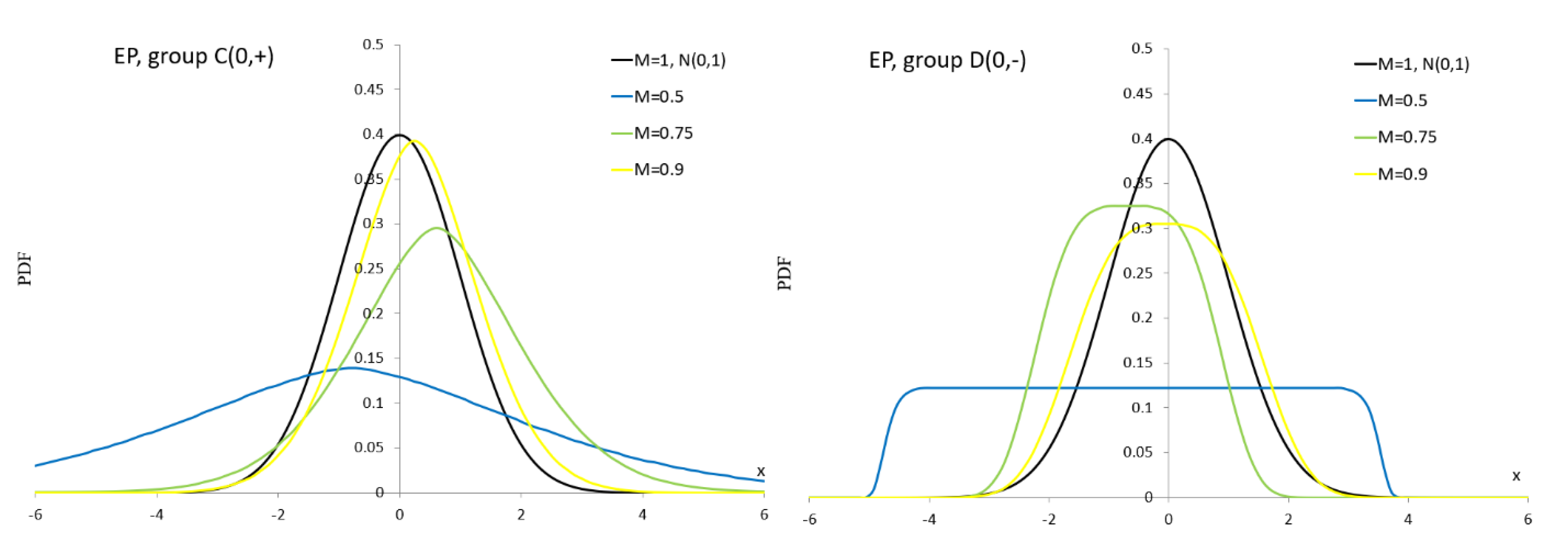
The fourth criterion for selecting an alternative for Monte Carlo simulation is that and calculated for the alternative parameters belong to the C-D groups. These symmetric alternatives can be very similar to the normal distribution. This criterion is fulfilled by the extended easily changeable kurtosis (EECK) distribution defined in finite domain and the exponential power (EP) distribution defined in an infinite domain.
PDFs of selected alternatives and their special cases are presented in Appendix.
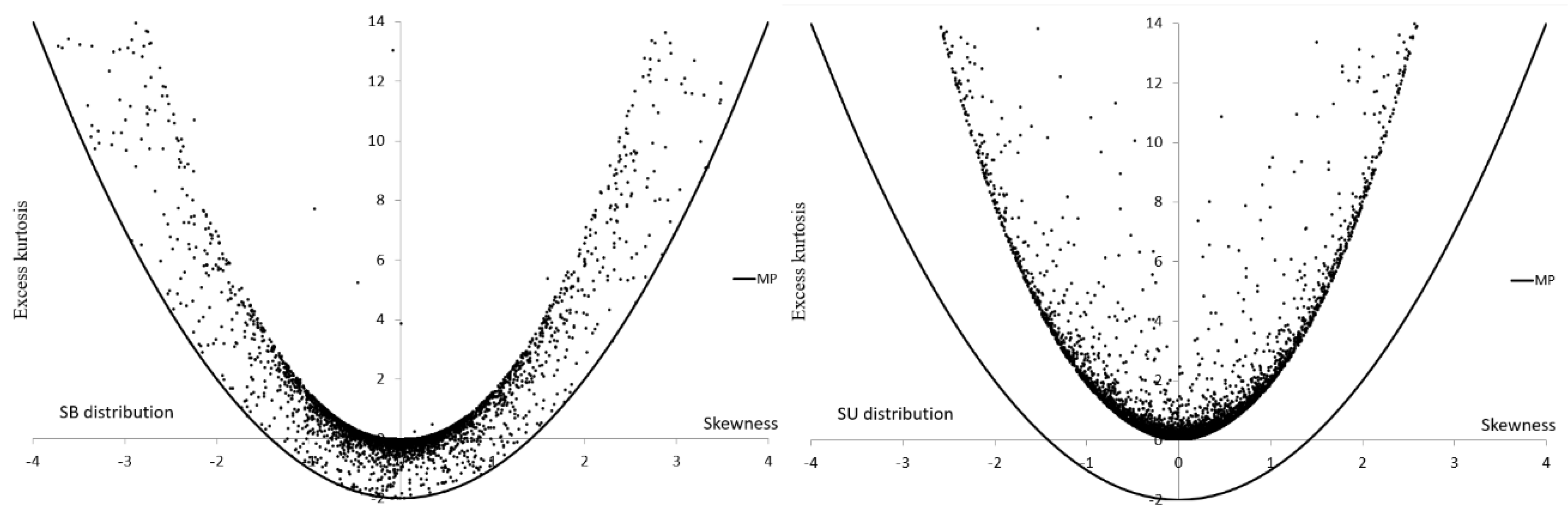
Let be coordinate of a point described by skewness and excess kurtosis, respectively. For every alternative, values of are calculated for randomly determined values of parameters influencing and in the Malakhov area (MA) [57]. If , then . The parameter ranges of the alternatives are selected to maximize MA filling (see Table 3). Figure 2, Figure 3, Figure 4 and Figure 5 present sets of points located in the MA for non-symmetric alternatives. It is interesting that the MA for SB and SU are separate, they complement each other.
We also calculate the skewness-kurtosis-square (SKS) measure necessary to compare the flexibility of alternatives. Circles of diameter and coordinates of their centers determined by and are placed within the MA. Then colored area fraction is calculated. Square sides equal to seem a reasonable alternative to circles since they simplify calculation of the total-colored area. Obviously, when some squares overlap, only one is taken into account. The SKS measure is given by [15]
where denotes a total number of squares within the MA, – a number of squares to which the point has fallen. The measure takes values in . The maximum value denotes a perfect dispersal of points in the MA.
Table 3 shows that the numerical ranges of and for asymmetric alternatives in the MA , due to the appropriately randomly selected parameter of the alternatives, except the SU, are similar. The range is not the most important. The interior is also important and therefore we also present values of SKS measures obtained for square side (see Table 4). Figure 3 and Table 4 confirm what could be expected, that the most flexible distributions are P and ES.
Figure 5.
A graphical range of and . The PCM and LM distributions.
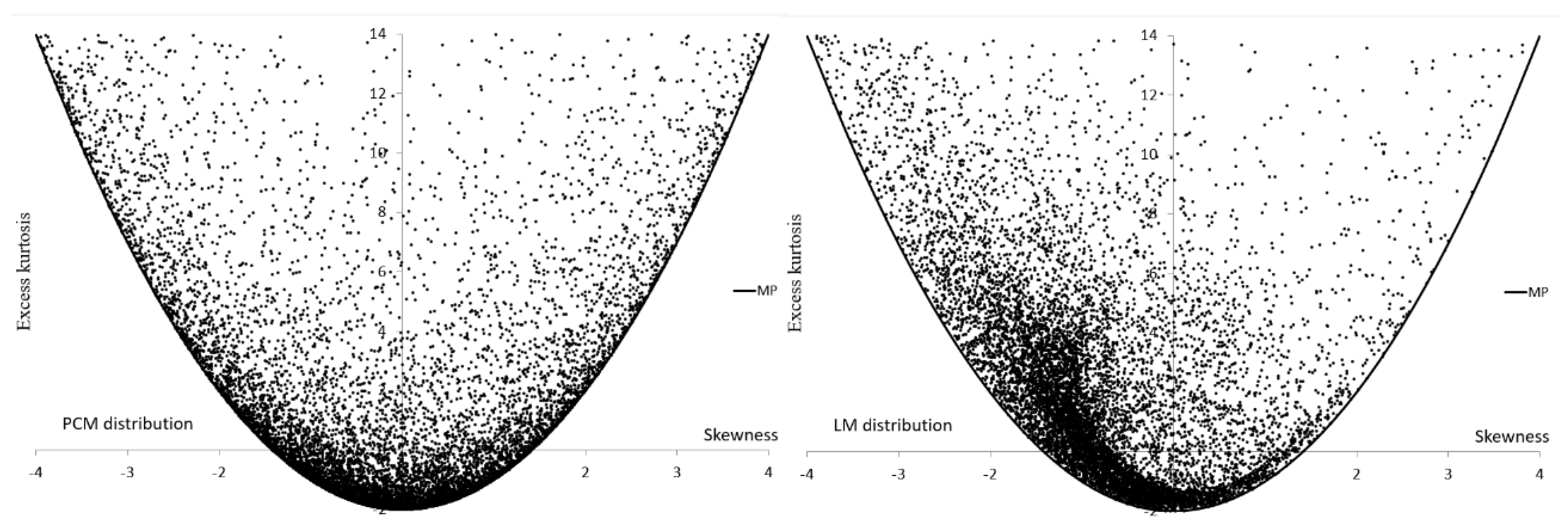
Figure 6.
A graphical range of and . The SB and SU distributions.
We choose values of alternative parameters to obtain the appropriate similarity measure M. Dominant values of this measure are .
Appendix presents Table A1–Table A10 with vectors of the alternative parameter , mean ,standard deviation , skewness , excess kurtosis and the similarity measure M for the analyzed alternatives. The skewness and excess kurtosis tend to zero, while the similarity measure tends to unity. Often, the mean tends to zero, and the standard deviation tends to unity, while the similarity measure tends to unity. PDF formulas and PDF curves (see Figure A1–Figure A10) for the alternative values are also provided in Appendix.
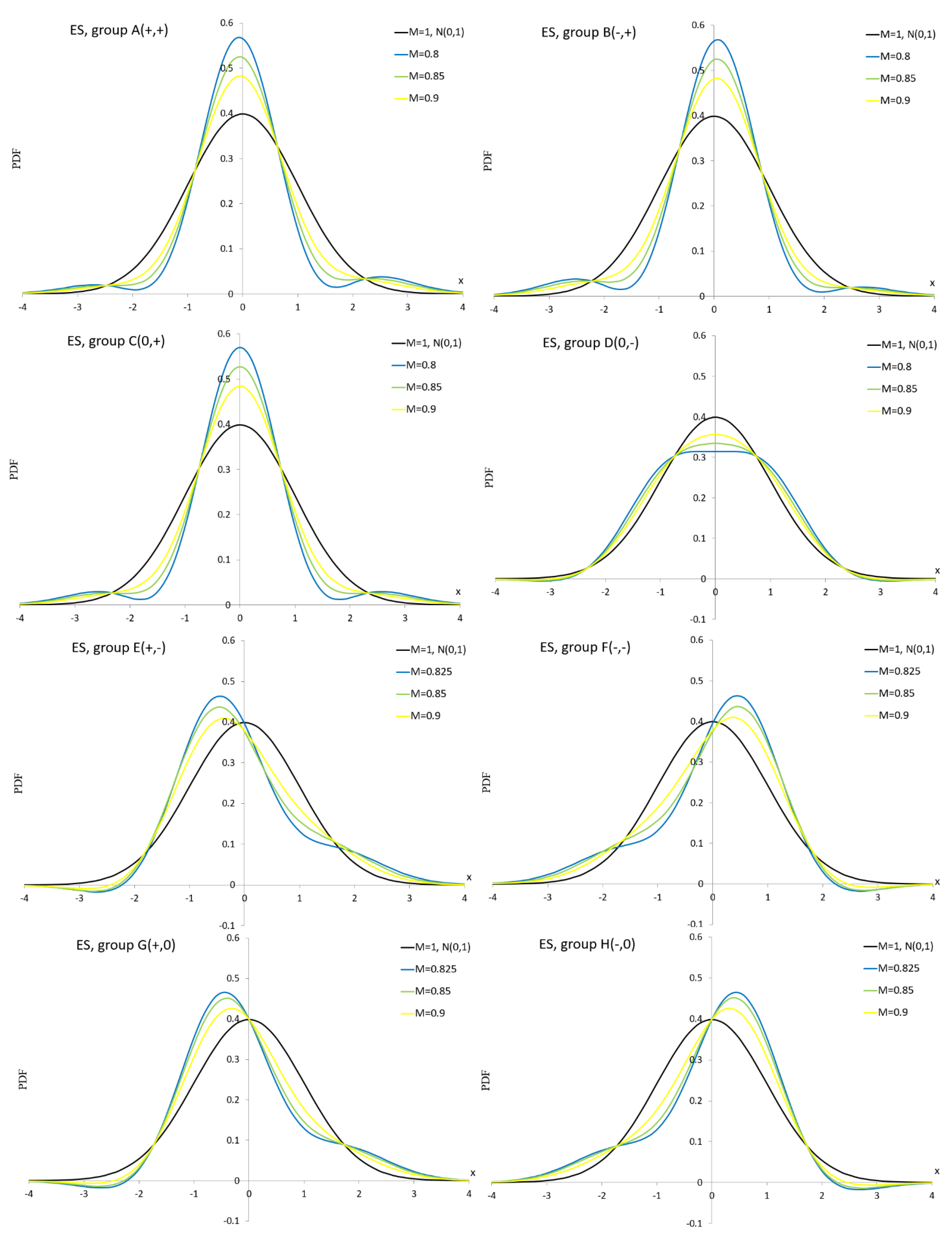
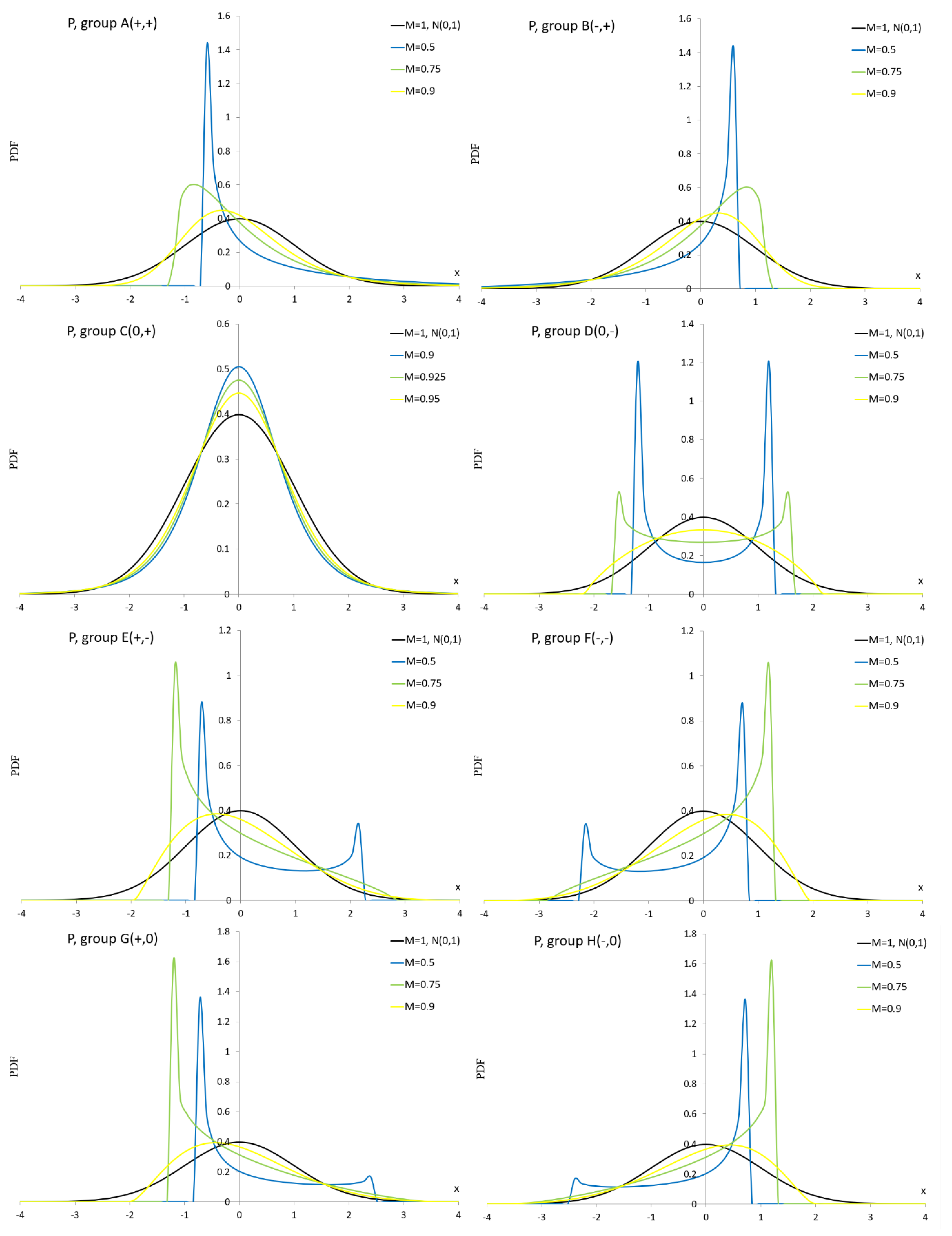
As can be seen in Figure A1, the ES distribution is not suitable for simulation studies for groups D–H because we observe negative PDF values even though the normalization condition is met. Figure A2 shows bathtub shapes. Figure A3, Figure A4 and Figure A6 show unimodal and bimodal shapes. In Figure A5 we can see very interesting multimodal shapes. In Figure A7 dominate unimodal shapes and Figure A8 shows only unimodal shapes. In Figure A9, we observe flat modes and in Figure A10, very flat modes with table shapes.
5. Power Study
In [34], a sample of the most recent comparisons (since 1990) has been used to rank 55 different normality tests. The overall winner of this analysis is the regression-based Shapiro-Wilk (SW) test of normality.
The parametrized KS (PKS) test with the statistic (6) was compared with the one-component LF test with the statistic (3), Shapiro–Wilk (SW) [61], Shapiro-Francia (SF) [62], AD and CM tests. To study the power of tests, critical values (the type I error equals ) were calculated using order statistics. The power of tests (PoTs) was calculated based on values of test statistics. Table 5 shows critical values (CVs) and test sizes (TSs) for sample sizes . The TS values are close to 0.05, so the simulation procedures are correct.
Complete simulation results with power values fill a table with 20 columns (20 tests) and 60 rows (10 alternatives, 2 sample sizes, 3 similarity measures). Presenting such large tables is difficult due to the size of the article. Therefore, the conclusions are applied to the full results, and only the most interesting results (tests with the highest power) will be shown in Table 6, Table 7, Table 8, Table 9, Table 10, Table 11, Table 12 and Table 13. Alternatives are indexed, i.e. the larger the index, the more the distribution resembles a normal distribution (e.g. index three denotes the similarity measure 0.9). The highest values are in bold.
Of course, it is expected that the power of the GoFTs increases as the sample size increases. This basic assumption is not met for the SB (groups C and D) and SU (groups D and E) alternatives. In these cases, the power is close to the significance level. It is expected that the power of the GoFTs decreases as the value of the similarity measure (7) increases. This basic assumption is not met for the P (groups A - H), PCM (groups C, D and H), LM (groups D and H), SB (groups C, D and H), SU (groups C, D, E, F and H) and EECK (group C) alternatives.
The average PoTs is the highest for group B alternatives, followed by groups E and F. This means that the GoFTs best detect samples from asymmetric distributions with positive excess kurtosis. The worst thing, as you might expect, is detecting samples from symmetric distributions. The GoFTs best detect samples from the Pearson distribution and the worst from the EECK distribution.
Based on the results from Table 6, Table 7, Table 8, Table 9, Table 10, Table 11, Table 12 and Table 13, we can conclude that and SF tests are the most powerful for the group A of alternatives; and SF tests are the most powerful for the group B of alternatives; SF test is the most powerful for the group C of alternatives; and tests are the most powerful for the group D of alternatives; test is the most powerful for the group E of alternatives; and SW tests are the most powerful for the group F of alternatives; test is the most powerful for the group G of alternatives and test is the most powerful for the group H of alternatives.
6. Real Data Examples
In this section, we present an application of the analyzed GoFT in real datasets to illustrate its potentiality. Details related to examples I – XXX are presented in Table 14.
When fitting the normal distribution to the data, we calculate p-values for the analyzed GoFTs based on statistic values (see Table 15, Table 16 and Table 17). The lowest p-value for the analyzed tests is in bold. The non-normality is the most pronounced by parameterized GoFTs, namely (example V), (examples I – III, V – VIII, XII, XIV, XV, XVII, XVIII, XXIV – XXVI, XXVIII and XXIX), (example V), (example V), (examples IV, XIII, XVI and XX), (examples IX, X, XI, XXII, XXIII, XXVII and XXX), (examples XIX and XXIII) and (examples X, XI and XXI).
7. Conclusions
The analyzed GoFTs detect samples from asymmetric distributions with positive excess kurtosis best and samples from symmetric distributions with positive excess kurtosis worst. The mentioned tests detect samples from a Pearson distribution best and those from the EP distribution worst.
The parameterized GoFT, called , stands out in the alternative groups A, E and G. The new parameterized KS GoFT stands out among the alternatives B , D, F , and H .
The good performance of the parameterized GoFTs, including the new proposal, was demonstrated by analyzing thirty real datasets.
Author Contributions
Conceptualization, D.S. and P.S.; methodology, P.S.; software, D.S. and P.S.; validation, D.S. and P.S.; formal analysis, P.S.; investigation, D.S. and P.S.; resources, D.S. and P.S.; data curation, D.S. and P.S.; writing—original draft preparation, D.S. and P.S.; writing—review and editing, D.S. and P.S.; visualization, D.S. and P.S.; supervision, P.S.; project administration, D.S. All authors have read and agreed to the published version of the manuscript.
Funding
This research received no external funding.
Informed Consent Statement
Not applicable.
Conflicts of Interest
The authors declare no conflicts of interest.
Abbreviations
The following abbreviations are used in this manuscript:
| A | Alternative distribution |
| AD | Anderson-Darling test |
| ALT | Alternative distribution |
| CDF | Cumulative distribution function |
| CM | Cramer-von Mises test |
| CV | Critical value |
| EDF | Empirical distribution function |
| EECK | Extended easily changeable kurtosis distribution |
| EP | Exponential power distribution |
| ES | Edgeworth series |
| GoFT | Goodness-of-fit test |
| K | Kuiper test |
| KS | Kolmogorov-Smirnov test |
| LF | Lilliefors test |
| M | Similarity measure |
| MA | Malakhov area |
| MCM | Modified Cramer-von Mises test |
| MSE | Mean square error |
| NDPC | Normal distribution with plasticizing component distribution |
| NM | Normal mixture distribution |
| P | Pearson distribution |
| PCM | Plasticizing component mixture distribution |
| Probability density function | |
| PKS | Parametrized KS test |
| PoT | Power of tests |
| SB | Johnson SB distribution |
| SKS | Skewness-kurtosis-square measure |
| SU | Johnson SU distribution |
| TS | Test size |
| Ts | Numbered tests |
| W | Watson test |
Appendix A
Appendix A.1. Edgeworth Series Distribution
PDF of the Edgeworth series (ES) with parameters and is given by [63]
where. We have , obviously.

Table A1.
Vectors of ES parameter , mean , standard deviation , skewness , excess kurtosis and similarity measure M. Groups 0, A-H.
Table A1.
Vectors of ES parameter , mean , standard deviation , skewness , excess kurtosis and similarity measure M. Groups 0, A-H.
| Group | ||||||
|---|---|---|---|---|---|---|
| 0 | 0 | 1 | 0 | 0 | ||
| A | (0.4,3.33) | 0 | 1 | 0.4 | 3.33 | |
| (0.3,2.499) | 0 | 1 | 0.3 | 2.499 | ||
| (0.2,1.666) | 0 | 1 | 0.2 | 1.666 | ||
| B | (-0.4,3.33) | 0 | 1 | -0.4 | 3.33 | |
| (-0.3,2.499) | 0 | 1 | -0.3 | 2.499 | ||
| (-0.2,1.666) | 0 | 1 | -0.2 | 1.666 | ||
| C | (0,3.428) | 0 | 1 | 0 | 3.428 | |
| (0,2.571) | 0 | 1 | 0 | 2.571 | ||
| (0,1.71) | 0 | 1 | 0 | 1.71 | ||
| D | (0,-3.428) | 0 | 1 | 0 | -3.428 | |
| (0,-2.571) | 0 | 1 | 0 | -2.571 | ||
| (0,-1.71) | 0 | 1 | 0 | -1.71 | ||
| E | (1.39,-0.067) | 0 | 1 | 1.39 | -0.067 | |
| (1.175,-0.46) | 0 | 1 | 1.175 | -0.46 | ||
| (0.775,-0.408) | 0 | 1 | 0.775 | -0.408 | ||
| F | (-1.39,-0.067) | 0 | 1 | -1.39 | -0.067 | |
| (-1.175,-0.46) | 0 | 1 | -1.175 | -0.46 | ||
| (-0.775,-0.408) | 0 | 1 | -0.775 | -0.408 | ||
| G | (1.391,0) | 0 | 1 | 1.391 | 0 | |
| (1.19,0) | 0 | 1 | 1.19 | 0 | ||
| (0.795,0) | 0 | 1 | 0.795 | 0 | ||
| H | (-1.391,0) | 0 | 1 | -1.391 | 0 | |
| (-1.19,0) | 0 | 1 | -1.19 | 0 | ||
| (-0.795,0) | 0 | 1 | -0.795 | 0 |
Figure A1.
PDF curves of the ES distribution for parameter values presented in Table A1.
Figure A1.
PDF curves of the ES distribution for parameter values presented in Table A1.
Appendix A.2. Pearson Distribution
Let
then the PDF of the Pearson (P) distribution is given by (Pearson 1895)
where and , , are normalizing constants defined as
A special case of the P distribution is the normal for .
Table A2.
Vectors of the P parameter , mean , standard deviation , skewness , excess kurtosis and similarity measure M. Groups 0, A-H.
Table A2.
Vectors of the P parameter , mean , standard deviation , skewness , excess kurtosis and similarity measure M. Groups 0, A-H.
| Group | ||||||
|---|---|---|---|---|---|---|
| 0 | (0,0) | 0 | 1 | 0 | 0 | |
| A | (2.04,4.1) | 0 | 1 | 2.04 | 4.1 | |
| (1.62,3.845) | 0 | 1 | 1.62 | 3.845 | ||
| (0.9,2) | 0 | 1 | 0.9 | 2 | ||
| B | (-2.04,4.1) | 0 | 1 | -2.04 | 4.1 | |
| (-1.62,3.845) | 0 | 1 | -1.62 | 3.845 | ||
| (-0.9,2) | 0 | 1 | -0.9 | 2 | ||
| C | (0,11.2) | 0 | 1 | 0 | 11.2 | |
| (0,3.65) | 0 | 1 | 0 | 3.65 | ||
| (0,1.521) | 0 | 1 | 0 | 1.521 | ||
| D | (0,-1.695) | 0 | 1 | 0 | -1.695 | |
| (0,-1.315) | 0 | 1 | 0 | -1.315 | ||
| (0,-0.89) | 0 | 1 | 0 | -0.89 | ||
| E | (0.985,-0.5) | 0 | 1 | 0.985 | -0.5 | |
| (0.715,-0.475) | 0 | 1 | 0.715 | -0.475 | ||
| (0.515,-0.2) | 0 | 1 | 0.515 | -0.2 | ||
| F | (-0.985,-0.5) | 0 | 1 | -0.985 | -0.5 | |
| (-0.715,-0.475) | 0 | 1 | -0.715 | -0.475 | ||
| (-0.515,-0.2) | 0 | 1 | -0.515 | -0.2 | ||
| G | (1.164,0) | 0 | 1 | 1.164 | 0 | |
| (0.879,0) | 0 | 1 | 0.879 | 0 | ||
| (0.578,0) | 0 | 1 | 0.578 | 0 | ||
| H | (-1.164,0) | 0 | 1 | -1.164 | 0 | |
| (-0.879,0) | 0 | 1 | -0.879 | 0 | ||
| (-0.578,0) | 0 | 1 | -0.578 | 0 |
Figure A2.
PDF curves of the P distribution for parameter values presented in Table A2.
Figure A2.
PDF curves of the P distribution for parameter values presented in Table A2.
Appendix A.3. Normal Mixture Distribution
PDF of the normal mixture (NM) distribution is given by
where and .
Special cases of the NM distribution are:
- normal for , for ,
- location contaminated normal (LCN) ,
- scale contaminated normal (SCN) .
Table A3.
Vectors of the NM parameter , mean , standard deviation , skewness , excess kurtosis and similarity measure M. Groups 0, A-H.
Table A3.
Vectors of the NM parameter , mean , standard deviation , skewness , excess kurtosis and similarity measure M. Groups 0, A-H.
| Group | ||||||
|---|---|---|---|---|---|---|
| 0 | 0 | 1 | 0 | 0 | ||
| 0 | 1 | 0 | 0 | |||
| A | (0.572,2.472,5.614,3.454,0.787) | 1.646 | 3.408 | 0.685 | 0.755 | |
| (-0.215,1.254,1.979,1.99,0.639) | 0.577 | 1.883 | 0.645 | 0.502 | ||
| (0.497,1.376,-0.268,0.884,0.612) | 0.2 | 1.265 | 0.287 | 0.249 | ||
| B | (0.502,2.019,1.708,0.953,0.36) | 1.274 | 1.544 | -0.748 | 1.502 | |
| (0.06,1.437,1.004,0.609,0.634) | 0.406 | 1.285 | -0.5 | 0.499 | ||
| (0.709,0.368,-0.072,1.115,0.193) | 0.079 | 1.06 | -0.301 | 0.15 | ||
| C | (0.519,6.599,0.519,1.058,0.665) | 0.519 | 5.416 | 0 | 1.398 | |
| (0.137,0.581,0.137,2.391,0.294) | 0.137 | 2.034 | 0 | 1.054 | ||
| (0.1,0.988,0.1,1.543,0.532) | 0.1 | 1.278 | 0 | 0.554 | ||
| D | (-0.511,1.353,4.293,1.021,0.551) | 1.645 | 2.681 | 0 | -1.28 | |
| (2.707,0.013,0.017,1.125,0.238) | 0.657 | 1.509 | 0 | -1.001 | ||
| (1.243,0.621,-0.39,0.811,0.347) | 0.111 | 1.09 | 0 | -0.63 | ||
| E | (-0.475,2.22,5.318,2.427,0.721) | 1.141 | 3.457 | 0.5 | -0.204 | |
| (-0.019,1.369,2.979,1.15,0.829) | 0.494 | 1.748 | 0.339 | -0.1 | ||
| (2.635,0.35,-0.015,1.166,0.038) | 0.086 | 1.253 | 0.137 | -0.075 | ||
| F | (-0.692,0.705,2.1,0.679,0.324) | 1.195 | 1.476 | -0.542 | -0.852 | |
| (-0.055,1.277,1.781,0.443,0.775) | 0.358 | 1.377 | -0.3 | -0.5 | ||
| (-0.09,1.08,-1.581,0.92,0.9) | -0.239 | 1.155 | -0.071 | -0.042 | ||
| G | (2.686,3.099,-0.964,2.217,0.471) | 0.755 | 3.232 | 0.4 | 0 | |
| (-0.56,1.465,1.411,1.45,0.8) | -0.166 | 1.661 | 0.151 | 0 | ||
| (-0.286,1.114,0.984,1.105,0.801) | -0.033 | 1.222 | 0.101 | 0 | ||
| H | (2.425,1.101,0.272,1.693,0.526) | 1.404 | 1.775 | -0.499 | 0 | |
| (0.864,1.125,-1.339,1.241,0.735) | 0.28 | 1.511 | -0.386 | 0 | ||
| (0.429,1.078,-0.364,1.228,0.434) | -0.02 | 1.23 | -0.1 | 0 |
Figure A3.
PDF curves of the NM distribution for parameter values presented in Table A3.
Figure A3.
PDF curves of the NM distribution for parameter values presented in Table A3.
Appendix A.4. Normal Distribution with Plasticizing Component
PDF of the normal distribution with plasticizing component (NDPC) is given by [64]
where and .
Special cases of the NDPC distribution are: for ; for and plasticizing component for .
Table A4.
Vectors of NDPC parameter , mean ,standard deviation , skewness , excess kurtosis and similarity measure M. Groups 0, A-H.
Table A4.
Vectors of NDPC parameter , mean ,standard deviation , skewness , excess kurtosis and similarity measure M. Groups 0, A-H.
| Group | ||||||
|---|---|---|---|---|---|---|
| 0 | () | 0 | 1 | 0 | 0 | |
| () | 0 | 1 | 0 | 0 | ||
| A | (1.194,0.601,2.186,2.592,2,0.666) | 1.526 | 1.5 | 1.002 | 1.001 | |
| (0.265,0.415,0.996,1.541,1.16,0.313) | 0.767 | 1.288 | 0.426 | 0.152 | ||
| (0.173,0.358,0.289,1.268,1.132,0.198) | 0.266 | 1.104 | 0.056 | 0.071 | ||
| B | (-1.321,1.842,0.741,0.459,2.56,0.287) | 0.15 | 1.4 | -1.764 | 3.3 | |
| (0.539,0.632,-1.078,2.061,1.174,0.741) | 0.12 | 1.34 | -1.499 | 2.986 | ||
| (-0.966,1.824,0.259,0.889,1.1,0.26) | -0.059 | 1.305 | -0.899 | 1.999 | ||
| C | (1.308,0.656,1.308,3.261,2,0.613) | 1.308 | 1.884 | 0 | 0.504 | |
| (0.571,1.023,0.571,1.962,1.15,0.505) | 0.571 | 1.508 | 0 | 0.325 | ||
| (-0.097,1.332,-0.097,1.058,1.1,0.614) | -0.097 | 1.223 | 0 | 0.101 | ||
| D | (-0.692,2.203,-0.692,2.544,1.759,0.25) | -0.692 | 2.265 | 0 | -1 | |
| (0.323,1.312,0.605,1.335,1.2,0.01) | 0.602 | 1.266 | 0 | -0.587 | ||
| (0.179,0.494,0.179,1.163,1.426,0.443) | 0.179 | 0.862 | 0 | -0.202 | ||
| E | (0.675,0.284,2.122,1.968,2.104,0.374) | 1.581 | 1.565 | 0.749 | -0.849 | |
| (0.423,1.032,1.058,2.077,1.815,0.494) | 0.744 | 1.544 | 0.311 | -0.667 | ||
| (-0.134,0.993,0.671,1.211,1.479,0.583) | 0.202 | 1.115 | 0.115 | -0.4 | ||
| F | (1.609,0.59,0.322,2.194,1.609,0.309) | 0.72 | 1.784 | -0.491 | -0.728 | |
| (0.617,0.737,0.129,1.752,1.465,0.332) | 0.291 | 1.395 | -0.239 | -0.526 | ||
| (-0.046,1.156,1.261,0.799,1.87,0.876) | 0.116 | 1.191 | -0.1 | -0.2 | ||
| G | (1.88,2.736,-0.848,1.122,6.437,0.679) | 1.005 | 2.656 | 0.524 | 0 | |
| (2.419,1.56,0.237,1.384,1.476,0.074) | 0.398 | 1.409 | 0.35 | 0 | ||
| (0.055,0.702,0.474,1.586,1.328,0.473) | 0.276 | 1.191 | 0.31 | 0 | ||
| H | (1.642,1.247,0.202,2.681,1.428,0.554) | 1 | 2.018 | -0.594 | 0 | |
| (-1.246,1.326,0.858,1.103,1.242,0.313) | 0.2 | 1.496 | -0.5 | 0 | ||
| (-0.115,1.286,0.306,1.091,1.093,0.465) | 0.11 | 1.189 | -0.1 | 0 |
Figure A4.
PDF curves of the NDPC for parameter values presented in Table A4.
Figure A4.
PDF curves of the NDPC for parameter values presented in Table A4.
Appendix A.5. Plasticizing Component Mixture Distribution
Special cases of the PCM distribution are: for ; for ; plasticizing components and for , respectively.
Table A5.
Vectors of PCM parameter , mean , standard deviation , skewness , excess kurtosis and similarity measure M. Groups 0, A-H.
Table A5.
Vectors of PCM parameter , mean , standard deviation , skewness , excess kurtosis and similarity measure M. Groups 0, A-H.
| Group | ||||||
|---|---|---|---|---|---|---|
| 0 | ) | 0 | 1 | 0 | 0 | |
| () | 0 | 1 | 0 | 0 | ||
| A | (1.415,1.684,2.194,11.252,5.474,2.331,0.9) | 2.399 | 3.622 | 2.647 | 7.663 | |
| (0.444,0.899,1.602,1.653,2.506,1.876,0.64) | 0.879 | 1.604 | 0.913 | 0.412 | ||
| (-0.076,1.056,1.1,0.701,1.646,1.095,0.71) | 0.149 | 1.268 | 0.374 | 0.374 | ||
| B | (1.366,0.572,1.11,0.502,1.669,1.253,0.658) | 1.071 | 1.099 | -0.978 | 1.565 | |
| (0.67,0.425,1.576,-0.323,1.696,1.05,0.349) | 0.024 | 1.444 | -0.569 | 0.606 | ||
| (-0.204,2.209,1.205,0.133,1.139,1.05,0.076) | 0.107 | 1.224 | -0.122 | 0.457 | ||
| C | (1.597,2.518,1.263,1.596,0.856,1.285,0.526) | 1.597 | 1.797 | 0 | 0.601 | |
| (0.012,0.274,1.256,0.012,2.046,1.01,0.183) | 0.012 | 1.846 | 0 | 0.598 | ||
| (0.127,1.089,1.01,0.127,0.183,1.01,0.863) | 0.127 | 1.01 | 0 | 0.401 | ||
| D | (1.631,0.893,1.05,1.632,2.104,1.554,0.498) | 1.632 | 1.488 | 0 | -0.268 | |
| (0.639,1.576,1.167,0.64,1.085,1.199,0.163) | 0.64 | 1.12 | 0 | -0.251 | ||
| (0.666,1.123,4.041,0.233,1.069,1.05,0.01) | 0.237 | 1.052 | 0 | -0.198 | ||
| E | (1.472,0.782,1.11,0.236,0.291,3.203,0.692) | 1.091 | 0.861 | 0.38 | -0.8 | |
| (-0.196,0.341,1.064,0.613,0.758,1.204,0.153) | 0.489 | 0.734 | 0.201 | -0.7 | ||
| (0.722,0.703,1.304,-0.57,0.598,1.05,0.455) | 0.018 | 0.893 | 0.179 | -0.617 | ||
| F | (0.261,1.419,1.909,3.099,0.744,1.567,0.57) | 1.481 | 1.757 | -0.3 | -1.107 | |
| (0.037,1.295,1.076,1.316,1.171,1.654,0.485) | 0.696 | 1.326 | -0.204 | -0.4 | ||
| (0.201,0.121,1.573,0.184,1.177,1.161,0.066) | 0.185 | 1.087 | -0.003 | -0.331 | ||
| G | (1.088,0.894,3.782,1.969,2.71,1.792,0.55) | 1.484 | 1.793 | 0.6 | 0 | |
| (1.515,2.553,3.55,0.07,1.328,1.619,0.07) | 0.171 | 1.359 | 0.501 | 0 | ||
| (-0.034,1.072,1.159,1.146,1.51,1.301,0.756) | 0.254 | 1.238 | 0.401 | 0 | ||
| H | (0.816,1.867,1.24,1.787,1.272,1.05,0.278) | 1.517 | 1.475 | -0.302 | 0 | |
| (-0.364,1.889,1.057,0.29,1.413,1.05,0.527) | -0.055 | 1.682 | -0.154 | 0 | ||
| (0.286,0.405,1.27,-0.263,1.261,1.05,0.112) | -0.202 | 1.188 | -0.128 | 0 |
Figure A5.
PDF curves of the PCM distribution for parameter values presented in Table A5.
Figure A5.
PDF curves of the PCM distribution for parameter values presented in Table A5.
Appendix A.6. Laplace Mixture Distribution
PDF of the Laplace mixture (LM) distribution is given by
where and .
Special cases of the LM distribution are Laplace (L) for and for .
Table A6.
Vectors of LM parameter , mean , standard deviation , skewness , excess kurtosis and similarity measure M. Groups A-H.
Table A6.
Vectors of LM parameter , mean , standard deviation , skewness , excess kurtosis and similarity measure M. Groups A-H.
| Group | ||||||
|---|---|---|---|---|---|---|
| A | (4.521,7.174,-0.757,1.959,0.313) | 0.895 | 6.594 | 1.172 | 9.074 | |
| (1.169,1.491,-0.019,0.849,0.56) | 0.646 | 1.863 | 0.4 | 3.454 | ||
| (0.452,0.818,-0.947,0.482,0.762) | 0.119 | 1.219 | 0.224 | 1.644 | ||
| B | (-0.358,0.405,-2.549,2.309,0.234) | -2.036 | 3.018 | -0.407 | 3.5 | |
| (0.94,0.335,-0.571,1.585,0.122) | -0.387 | 2.164 | -0.202 | 3.136 | ||
| (-0.736,0.911,0.04,0.878,0.132) | -0.062 | 1.275 | -0.034 | 2.773 | ||
| C | (1.445,1.571,-2.516,1.87,1) | 1.445 | 2.222 | 0 | 3 | |
| (0.246,0.844,-0.59,0.905,0.043) | -0.554 | 1.287 | 0 | 2.894 | ||
| (0.319,0.86,-0.21,0.874,0.222) | -0.092 | 1.251 | 0 | 2.815 | ||
| D | (-6.131,0.945,-0.386,1.54,0.366) | -2.487 | 3.364 | 0 | -0.648 | |
| (-4.898,0.343,-0.415,1.234,0.29) | -1.716 | 2.523 | 0 | -0.597 | ||
| (2.115,0.07,-0.512,0.822,0.208) | 0.034 | 1.486 | 0 | -0.005 | ||
| E | (7.186,1.509,-0.869,0.58,0.309) | 1.62 | 3.966 | 1.005 | -0.403 | |
| (-1.711,0.177,0.773,0.823,0.421) | -0.274 | 1.522 | 0.5 | -0.32 | ||
| (1.023,0.358,-0.118,0.348,0.428) | 0.37 | 0.753 | 0.15 | -0.014 | ||
| F | (-3.863,0.348,1.522,1.359,0.248) | 0.184 | 2.872 | -0.18 | -0.556 | |
| (0.006,0.065,0.703,0.189,0.227) | 0.545 | 0.378 | -0.17 | -0.286 | ||
| (-0.466,0.161,0.08,0.159,0.48) | -0.182 | 0.354 | -0.05 | -0.2 | ||
| G | (2.309,1.022,-1.1,0.418,0.391) | 0.233 | 1.949 | 0.85 | 0 | |
| (-0.208,1.335,7.917,1.899,0.712) | 2.132 | 4.261 | 0.839 | 0 | ||
| (0.679,0.702,-1.434,0.642,0.532) | -0.31 | 1.422 | 0.036 | 0 | ||
| H | (-9.234,0.124,1.581,2.321,0.161) | -0.159 | 4.983 | -0.556 | 0 | |
| (-1.322,0.83,2.398,1.181,0.291) | 1.317 | 2.287 | -0.1 | 0 | ||
| (0.81,0.479,2.254,0.229,0.736) | 1.191 | 0.878 | -0.032 | 0 |
Figure A6.
PDF curves of the LM distribution for parameter values presented in Table A6.
Figure A6.
PDF curves of the LM distribution for parameter values presented in Table A6.
Appendix A.7. Johnson SB Distribution
PDF of the Johnson SB (SB) distribution is given by [65]
where.
Table A7.
Vectors of the SB parameter , mean ,standard deviation , skewness , excess kurtosis and similarity measure M. Groups A –B, D –H.
Table A7.
Vectors of the SB parameter , mean ,standard deviation , skewness , excess kurtosis and similarity measure M. Groups A –B, D –H.
| Group | ||||||
|---|---|---|---|---|---|---|
| A | (1.972,1.819,-0.45,4) | 0.613 | 0.411 | 0.649 | 0.3 | |
| (2.482,2.23,-1.665,7.423) | 0.237 | 0.618 | 0.584 | 0.298 | ||
| (3.092,2.702,-2.908,12.271) | 0.132 | 0.832 | 0.518 | 0.267 | ||
| B | (-4.086,2.097,-5.424,6.348) | 0.074 | 0.351 | -1 | 1.488 | |
| (-2.614,2.258,-5.722,7.58) | -0.021 | 0.611 | -0.6 | 0.341 | ||
| (-1.992,2.198,-6.446,8.974) | -0.129 | 0.823 | -0.485 | 0.099 | ||
| D | (0,3.149,-2.116,4.115) | -0.059 | 0.319 | 0 | -0.176 | |
| (0,3.958,-4.707,9.414) | 0 | 0.585 | 0 | -0.117 | ||
| (0,4.304,-8.154,15.856) | -0.227 | 0.909 | 0 | -0.1 | ||
| E | (0.664,0.45,-0.027,4.679) | 1.377 | 1.38 | 0.856 | -0.558 | |
| (0.834,0.754,-0.727,3.258) | 0.26 | 0.726 | 0.788 | -0.25 | ||
| (0.867,2.297,-4.627,10.828) | -0.18 | 1.095 | 0.2 | -0.227 | ||
| F | (-0.716,0.448,-0.622,1.618) | 0.534 | 0.47 | -0.931 | -0.4 | |
| (-1.044,1.22,-4.394,5.493) | -0.665 | 0.88 | -0.603 | -0.145 | ||
| (-1.202,1.515,-4.252,6.217) | -0.065 | 0.837 | -0.522 | -0.1 | ||
| G | (1.64,2.044,-3.761,8.045) | -1.199 | 0.819 | 0.452 | 0 | |
| (1.825,2.345,-1.984,6.623) | 0.145 | 0.596 | 0.401 | 0 | ||
| (2.952,4.082,-5.487,16.27) | -0.135 | 0.87 | 0.24 | 0 | ||
| H | (-1.357;1.565;-1.601;3.202) | 0.605 | 0.41 | -0.563 | 0 | |
| (-2.046;2.695;-5.081;7.468) | -0.032 | 0.592 | -0.354 | 0 | ||
| (-2.068;2.73;-7.098;10.398) | -0.07 | 0.814 | -0.35 | 0 |
Figure A7.
PDF curves of the SB distribution for parameter values presented in Table A7.
Figure A7.
PDF curves of the SB distribution for parameter values presented in Table A7.

Appendix A.8. Johnson SU Distribution
PDF of the Johnson SU (SU) distribution is given by [65]
where .
Table A8.
Vectors of the SU parameter , mean , standard deviation , skewness , excess kurtosis and similarity measure M. Groups A – C, E – H.
Table A8.
Vectors of the SU parameter , mean , standard deviation , skewness , excess kurtosis and similarity measure M. Groups A – C, E – H.
| Group | ||||||
|---|---|---|---|---|---|---|
| A | (-1.246,2.021,0.257,0.731) | 0.800 | 0.501 | 1.014 | 2.911 | |
| (-0.569,2.063,-1.301,2.625) | -0.477 | 1.499 | 0.493 | 1.720 | ||
| (-0.11,2.762,-0.069,3.319) | 0.072 | 1.286 | 0.049 | 0.648 | ||
| B | (2.502,2.889,2.029,3.828) | -1.949 | 2 | -0.8 | 1.455 | |
| (2.564,3.308,2.137,1.902) | 0.435 | 0.8 | -0.636 | 0.926 | ||
| (2.296,5.558,2.36,6.031) | -0.246 | 1.2 | -0.218 | 0.2 | ||
| C | (0,1.821,-1.617,3.096) | -1.617 | 1.992 | 0 | 2 | |
| (0,1.829,-0.205,2.967) | -0.205 | 1.897 | 0 | 1.97 | ||
| (0,3.372,0.204,2.935) | 0.204 | 0.91 | 0 | 0.403 | ||
| E | (-22.518,45.262,-11.095,19.766) | -0.848 | 0.492 | 0.031 | -0.007 | |
| (1.29,40.539,-0.294,-17.564) | 0.155 | 0.484 | 0.491 | -0.784 | ||
| (0.244,21.027,-0.134,-12.383) | 0.01 | 0.59 | 0.002 | -0.007 | ||
| F | (0.861,18.997,-1.158,14.674) | -1.824 | 0.774 | -0.011 | -0.005 | |
| (0.756,3.676,0.166,0.819) | -0.010 | 0.236 | -0.359 | -0.450 | ||
| (13.843,36.36,4.174,11.623) | -0.360 | 0.343 | -0.030 | -0.077 | ||
| G | (-9.342,11.021,-1.575,1.981) | 0.32 | 0.25 | 0.207 | 0 | |
| (-23.944,18.041,-8.486,5.409) | 1.009 | 0.606 | 0.15 | 0 | ||
| (-9.349,85.071,-3.763,35.754) | 0.174 | 0.423 | 0.004 | 0 | ||
| H | (0.738,49.723,3.6,73.029) | 2.516 | 1.469 | -0.001 | 0 | |
| (2.547,7.276,0.835,1.65) | 0.24 | 0.243 | -0.141 | 0 | ||
| (4.211,10.507,1.959,3.55) | 0.491 | 0.367 | -0.11 | 0 |
Figure A8.
PDF curves of the SU distribution for parameter values presented in Table A8.
Figure A8.
PDF curves of the SU distribution for parameter values presented in Table A8.
Appendix A.9. Extended Easily Changeable Kurtosis Distribution
PDF of the extended easily changeable kurtosis (EECK) distribution is given by [66]
where . Special cases of the EECK distribution are: uniform , triangle and easily changeable kurtosis [67] distributions.
Table A9.
Vectors of the EECK parameter , mean ,standard deviation , skewness , excess kurtosis and similarity measure M. Groups A-H.
Table A9.
Vectors of the EECK parameter , mean ,standard deviation , skewness , excess kurtosis and similarity measure M. Groups A-H.
| Group | ||||||
|---|---|---|---|---|---|---|
| C | (46.018,1.043) | 0 | 0.032 | 0 | 2.256 | |
| (40.914,1.366) | 0 | 0.06 | 0 | 0.921 | ||
| (10.676,1.184) | 0 | 0.128 | 0 | 0.912 | ||
| D | (60.495,4.846) | 0 | 0.244 | 0 | -0.921 | |
| (48.76,2.738) | 0 | 0.15 | 0 | -0.51 | ||
| (48.76,2.211) | 0 | 0.115 | 0 | -0.238 |
Figure A9.
PDF curves of the EECK distribution for parameter values presented in Table A9.
Figure A9.
PDF curves of the EECK distribution for parameter values presented in Table A9.
Appendix A.10. Exponential Power Distribution
Special case of the EP distribution is the for .
Table A10.
Vectors of the EP parameter , mean ,standard deviation , skewness , excess kurtosis and similarity measure M.
Table A10.
Vectors of the EP parameter , mean ,standard deviation , skewness , excess kurtosis and similarity measure M.
| Group | ||||||
|---|---|---|---|---|---|---|
| C | (-0.796,2.985,1.609) | -0.796 | 3.257 | 0 | 0.536 | |
| (90.611,1.385,1.695) | 0.611 | 1.478 | 0 | 0.386 | ||
| (90.251,1.033,1.785) | 0.251 | 1.079 | 0 | 0.253 | ||
| D | (-0.611,3.71,28.792) | -0.611 | 2.368 | 0 | -1.188 | |
| (-0.673,1.198,3.828) | -0.673 | 0.994 | 0 | -0.783 | ||
| (-0.05,1.272,3.117) | -0.05 | 1.11 | 0 | -0.619 |
Figure A10.
PDF curves of the EP distribution for parameter values presented in Table A10.
Figure A10.
PDF curves of the EP distribution for parameter values presented in Table A10.
References
- Kolmogorov, A.N. Sulla Determinazione Empirica di una Legge di Distribuzione. Giornale dell’Istituto Italiano degli Attuari 1933, 4, 83–91. [Google Scholar]
- Smirnov, N.V. Tabled distribution of the Kolmogorov–Smirnov statistic (sample). Annals of Mathematical Statistics 1948, 19, 279–281. [Google Scholar] [CrossRef]
- Cramér, H. On the Composition of Elementary Errors. Scandinavian Actuarial Journal 1928, 1, 13–74. [Google Scholar] [CrossRef]
- von Mises, R.E. Wahrscheinlichkeit, Statistik und Wahrheit; Julius Springer: Berlin, Germany, 1931. [Google Scholar]
- Lilliefors, H.W. On the Kolmogorov–Smirnov test for normality with mean and variance unknown. Journal of the American Statistical Association 1967, 62, 399–402. [Google Scholar] [CrossRef]
- Kuiper, N.H. Tests concerning random points on a circle. Proceedings of the Koninklijke Nederlandse Akademie van Wetenschappen, Series A 1960, 63, 38–47. [Google Scholar] [CrossRef]
- Watson, G.S. Goodness-of-fit tests on a circle (Part II). Biometrika 1962, 49((1–2)), 57–63. [Google Scholar] [CrossRef]
- Anderson, T.W.; Darling, D.A. Asymptotic Theory of Certain “Goodness-of-Fit” Criteria Based on Stochastic Processes. Annals of Mathematical Statistics 1952, 23, 193–212. [Google Scholar] [CrossRef]
- Harter, H.L.; Khamis, H.J.; Lamb, R.E. Modified Kolmogorov–Smirnov Tests of Goodness of Fit. Communications in Statistics–Simulation and Computation 1984, 13, 293–323. [Google Scholar] [CrossRef]
- Khamis, H.J. The δ-Corrected Kolmogorov–Smirnov Test for Goodness of Fit. Journal of Statistical Planning and Inference 1990, 24, 317–335. [Google Scholar] [CrossRef]
- Khamis, H.J. The δ-Corrected Kolmogorov–Smirnov Test with Estimated Parameters. Journal of Nonparametric Statistics 1992, 2, 17–27. [Google Scholar] [CrossRef]
- Khamis, H.J. A Comparative Study of the δ-Corrected Kolmogorov–Smirnov Test. Journal of Applied Statistics 1993, 20, 401–421. [Google Scholar] [CrossRef]
- Bloom, G. Statistical Estimates and Transformed Beta Variables; Wiley: New York, NY, USA, 1958. [Google Scholar]
- Sulewski, P. Modified Lilliefors goodness-of-fit test for normality. Communications in Statistics–Simulation and Computation 2020, 51, 1199–1219. [Google Scholar] [CrossRef]
- Sulewski, P. Two component modified Lilliefors test for normality. Equilibrium. Quarterly Journal of Economics and Economic Policy 2021, 16, 429–455. [Google Scholar] [CrossRef]
- Sulewski, P.; Stoltmann, D. Modified Cramér–von Mises goodness-of-fit test for normality. Przegląd Statystyczny 2023, 70, 1–36. [Google Scholar] [CrossRef]
- Filliben, J.J. The Probability Plot Correlation Coefficient Test for Normality. Technometrics 1975, 17, 111–117. [Google Scholar] [CrossRef]
- Bonett, D.G.; Seier, E. A Test of Normality with High Uniform Power. Computational Statistics and Data Analysis 2002, 40, 435–445. [Google Scholar] [CrossRef]
- Afeez, B.M.; Maxwell, O.; Otekunrin, O.; Happiness, O. Selection and Validation of Comparative Study of Normality Test. American Journal of Mathematics and Statistics 2018, 8, 190–201. [Google Scholar]
- Aliaga, A.M.; Martínez-González, E.; Cayón, L.; Argüeso, F.; Sanz, J.L.; Barreiro, R.B. Goodness-of-Fit Tests of Gaussianity: Constraints on the Cumulants of the MAXIMA Data. New Astronomy Reviews 2003, 47(8–10), 821–826.
- Marange, C.; Qin, Y. An empirical likelihood ratio based comparative study on tests for normality of residuals in linear models. Advances in Methodology and Statistics 2019, 16, 1–16. [Google Scholar] [CrossRef]
- Bontemps, C.; Meddahi, N. Testing Normality: A GMM Approach. Journal of Econometrics 2005, 124, 149–186. [Google Scholar] [CrossRef]
- Sulewski, P. Modification of Anderson–Darling goodness-of-fit test for normality. Afinidad 2019, 76, 588. [Google Scholar]
- Luceno, A. Fitting the generalized Pareto distribution to data using maximum goodness-of-fit estimators. Computational Statistics & Data Analysis 2006, 51, 904–917. [Google Scholar]
- Tavakoli, M.; Arghami, N.; Abbasnejad, M. A goodness-of-fit test for normality based on Balakrishnan–Sanghvi information. Journal of the Iranian Statistical Society 2019, 18, 177–190. [Google Scholar] [CrossRef]
- Yazici, B.; Yolacan, S.A. Comparison of various tests of normality. Journal of Statistical Computation and Simulation 2007, 77, 175–183. [Google Scholar] [CrossRef]
- Mishra, P.; Pandey, C.M.; Singh, U.; Gupta, A.; Sahu, C.; Keshri, A. Descriptive statistics and normality tests for statistical data. Annals of Cardiac Anaesthesia 2019, 22, 67–74. [Google Scholar] [CrossRef]
- Gel, Y.R.; Miao, W.; Gastwirth, J.L. Robust Directed Tests of Normality against Heavy-Tailed Alternatives. Computational Statistics & Data Analysis 2007, 51, 2734–2746. [Google Scholar] [CrossRef]
- Kellner, J.; Celisse, A. A One-Sample Test for Normality with Kernel Methods. Bernoulli 2019, 25, 1816–1837. [Google Scholar] [CrossRef]
- Coin, D. A Goodness-of-Fit Test for Normality Based on Polynomial Regression. Computational Statistics and Data Analysis 2008, 52, 2185–2198. [Google Scholar] [CrossRef]
- Wijekularathna, D.K.; Manage, A.B.; Scariano, S.M. Power analysis of several normality tests: A Monte Carlo simulation study. Communications in Statistics–Simulation and Computation 2020, 51, 757–773. [Google Scholar] [CrossRef]
- Brys, G.; Hubert, M.; Struyf, A. Goodness-of-Fit Tests Based on a Robust Measure of Skewness. Computational Statistics 2008, 23, 429–442. [Google Scholar] [CrossRef]
- Gel, Y.R.; Gastwirth, J.L. A Robust Modification of the Jarque–Bera Test of Normality. Economics Letters 2008, 99, 30–32. [Google Scholar] [CrossRef]
- Hernandez, H. Testing for Normality: What Is the Best Method. ForsChem Research Reports 2021, 6, 2021–05. [Google Scholar]
- Romao, X.; Delgado, R.; Costa, A. An empirical power comparison of univariate goodness-of-fit tests of normality. Journal of Statistical Computation and Simulation 2010, 80, 545–591. [Google Scholar] [CrossRef]
- Khatun, N. Applications of Normality Test in Statistical Analysis. Open Journal of Statistics 2021, 11, 113–123. [Google Scholar] [CrossRef]
- Razali, N.M.; Wah, Y.B. Power comparisons of Shapiro–Wilk, Kolmogorov–Smirnov, Lilliefors and Anderson–Darling tests. Journal of Statistical Modeling and Analytics 2011, 2, 21–33. [Google Scholar]
- Arnastauskaitė, J.; Ruzgas, T.; Bražėnas, M. An Exhaustive Power Comparison of Normality Tests. Mathematics 2021, 9, 788. [Google Scholar] [CrossRef]
- Noughabi, H.A.; Arghami, N.R. Monte Carlo comparison of seven normality tests. Journal of Statistical Computation and Simulation 2011, 81, 965–972. [Google Scholar] [CrossRef]
- Bayoud, H.A. Tests of Normality: New Test and Comparative Study. Communications in Statistics–Simulation and Computation 2021, 50, 4442–4463. [Google Scholar] [CrossRef]
- Yap, B.W.; Sim, C.H. Comparisons of various types of normality tests. Journal of Statistical Computation and Simulation 2011, 81, 2141–2155. [Google Scholar] [CrossRef]
- Uhm, T.; Yi, S. A comparison of normality testing methods by empirical power and distribution of p-values. Communications in Statistics–Simulation and Computation 2021, 1–14.
- Chernobai, A.; Rachev, S.T.; Fabozzi, F.J. Composite Goodness-of-Fit Tests for Left-Truncated Loss Samples. In Handbook of Financial Econometrics and Statistics; Lee, C.-F., Ed.; Springer: New York, NY, USA, 2012; pp. 575–596. [Google Scholar]
- Sulewski, P. Two-piece power normal distribution. Communications in Statistics–Theory and Methods 2021, 50, 2619–2639. [Google Scholar] [CrossRef]
- Ahmad, F.; Khan, R.A. A Power Comparison of Various Normality Tests. Pakistan Journal of Statistics and Operation Research 2015, 11, 331–345. [Google Scholar] [CrossRef]
- Desgagné, A.; Lafaye de Micheaux, P.; Ouimet, F. Goodness-of-Fit Tests for Laplace, Gaussian and Exponential Power Distributions Based on λ-th Power Skewness and Kurtosis. Statistics 2022, 56, 1–29. [Google Scholar] [CrossRef]
- Mbah, A.K.; Paothong, A. Shapiro–Francia test compared to other normality tests using expected p-value. Journal of Statistical Computation and Simulation 2015, 85, 3002–3016. [Google Scholar] [CrossRef]
- Uyanto, S.S. An extensive comparison of 50 univariate goodness-of-fit tests for normality. Austrian Journal of Statistics 2022, 51, 45–97. [Google Scholar] [CrossRef]
- Torabi, H.; Montazeri, N.H.; Grane, A. A test of normality based on the empirical distribution function. SORT 2016, 40, 55–88. [Google Scholar]
- Ma, Y.; Kitani, M.; Murakami, H. On modified Anderson–Darling test statistics with asymptotic properties. Communications in Statistics–Theory and Methods 2024, 53, 1420–1439. [Google Scholar] [CrossRef]
- Feuerverger, A. On Goodness of Fit for Operational Risk. International Statistical Review 2016, 84, 434–455. [Google Scholar] [CrossRef]
- Giles, D.E. New Goodness-of-Fit Tests for the Kumaraswamy Distribution. Stats 2024, 7, 373–389. [Google Scholar] [CrossRef]
- Nosakhare, U.H.; Bright, A.F. Evaluation of techniques for univariate normality test using Monte Carlo simulation. American Journal of Theoretical and Applied Statistics 2017, 6((5–1)), 51–61. [Google Scholar]
- Borrajo, M.I.; González-Manteiga, W.; Martínez-Miranda, M.D. Goodness-of-Fit Test for Point Processes First-Order Intensity. Computational Statistics & Data Analysis 2024, 194, 107929. [Google Scholar]
- Desgagné, A.; Lafaye de Micheaux, P. A Powerful and Interpretable Alternative to the Jarque–Bera Test of Normality Based on 2nd-Power Skewness and Kurtosis, Using the Rao’s Score Test on the APD Family. Journal of Applied Statistics 2018, 45, 2307–2327. [Google Scholar] [CrossRef]
- Terán-García, E.; Pérez-Fernández, R. A robust alternative to the Lilliefors test of normality. Journal of Statistical Computation and Simulation 2024, 1–19. [Google Scholar] [CrossRef]
- Malachov, A.N. A Cumulant Analysis of Random Non-Gaussian Processes and Their Transformations; Soviet Radio: Moscow, 1978. [Google Scholar]
- Esteban, M.D.; Castellanos, M.E.; Morales, D.; Vajda, I. Monte Carlo Comparison of Four Normality Tests Using Different Entropy Estimates. Communications in Statistics–Simulation and Computation 2001, 30, 285–761. [Google Scholar] [CrossRef]
- Gan, F.F.; Koehler, K.J. Goodness-of-Fit Tests Based on P–P Probability Plots. Technometrics 1990, 32, 289–303. [Google Scholar] [CrossRef]
- Krauczi, E. A study of the quantile correlation test of normality. TEST: An Official Journal of the Spanish Society of Statistics and Operations Research 2009, 18, 156–165. [Google Scholar] [CrossRef]
- Shapiro, S.S.; Wilk, M.B. An analysis of variance test for normality. Biometrika 1965, 52, 591–611. [Google Scholar] [CrossRef]
- Shapiro, S.S.; Francia, R.S. An approximate analysis of variance test for normality. Journal of the American Statistical Association 1972, 67, 215–216. [Google Scholar] [CrossRef]
- Stuart, A.; Kendall, M.G. The Advanced Theory of Statistics; Hafner Publishing Company: New York, 1968. [Google Scholar]
- Sulewski, P. Normal distribution with plasticizing component. Communications in Statistics–Theory and Methods 2022, 51, 3806–3835. [Google Scholar] [CrossRef]
- Johnson, N.L. Systems of Frequency Curves Generated by Methods of Translation. Biometrika 1949, 36, 149–176. [Google Scholar] [CrossRef]
- Sulewski, P. Extended Easily Changeable Kurtosis Distribution. REVSTAT–Statistical Journal, accepted December 2023.
- Sulewski, P. Easily Changeable Kurtosis Distribution. Austrian Journal of Statistics 2023, 52, 1–24. [Google Scholar] [CrossRef]
- Lunetta, G. Di una generalizzazione dello schema della curva normale. Annali della Facoltà di Economia e Commercio di Palermo 1963, 17, 237–244. [Google Scholar]
- Kendall, M.G.; Stuart, A. The Advanced Theory of Statistics: Distribution Theory, Vol. 1; Hafner Publishing Company: New York, NY, USA, 1968. [Google Scholar]
- Subbotin, M.T. On the law of frequency of errors. Matematicheskii Sbornik 1923, 31, 296–301. [Google Scholar]
- Pearson, K. Memoir on skew variation in homogeneous material. Philosophical Transactions of the Royal Society of London, Series A 1895, 186, 343–414. [Google Scholar]
Figure 1.
Graphical representation of EDF definitions.
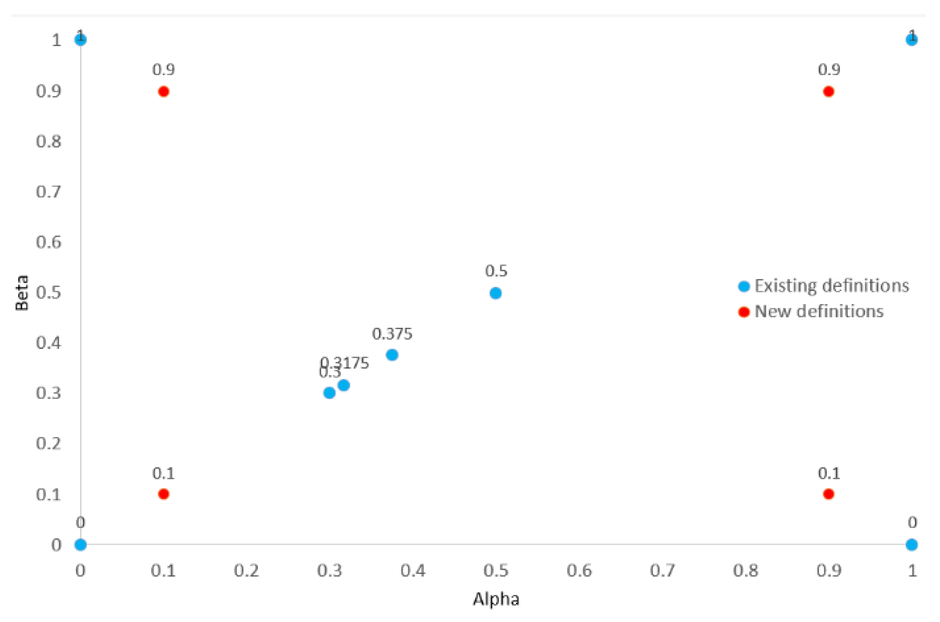
Figure 2.
Similarity measure for Student t distribution with v degrees of freedom.
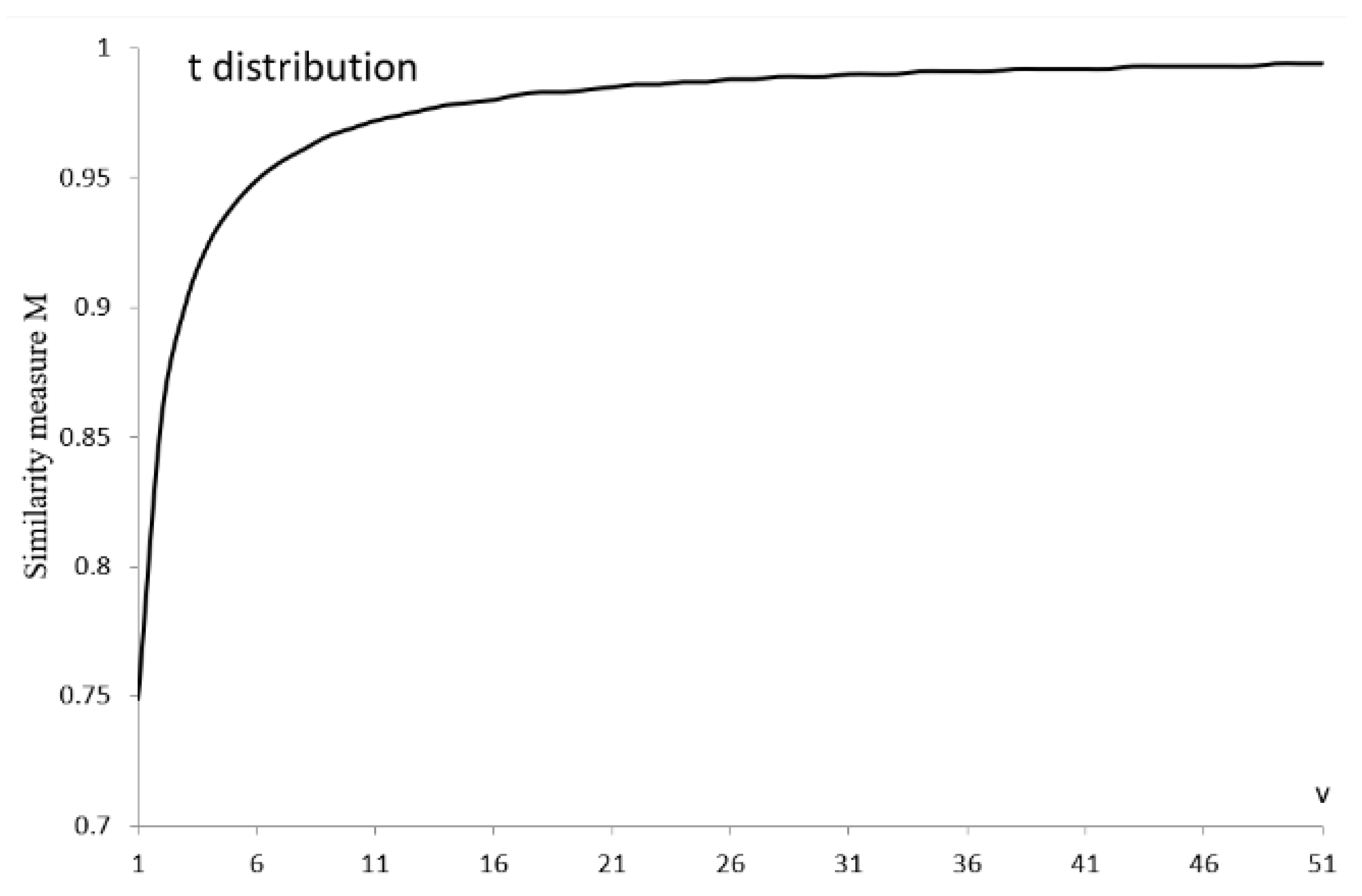
Figure 3.
A graphical range of and . The ES and P distributions.
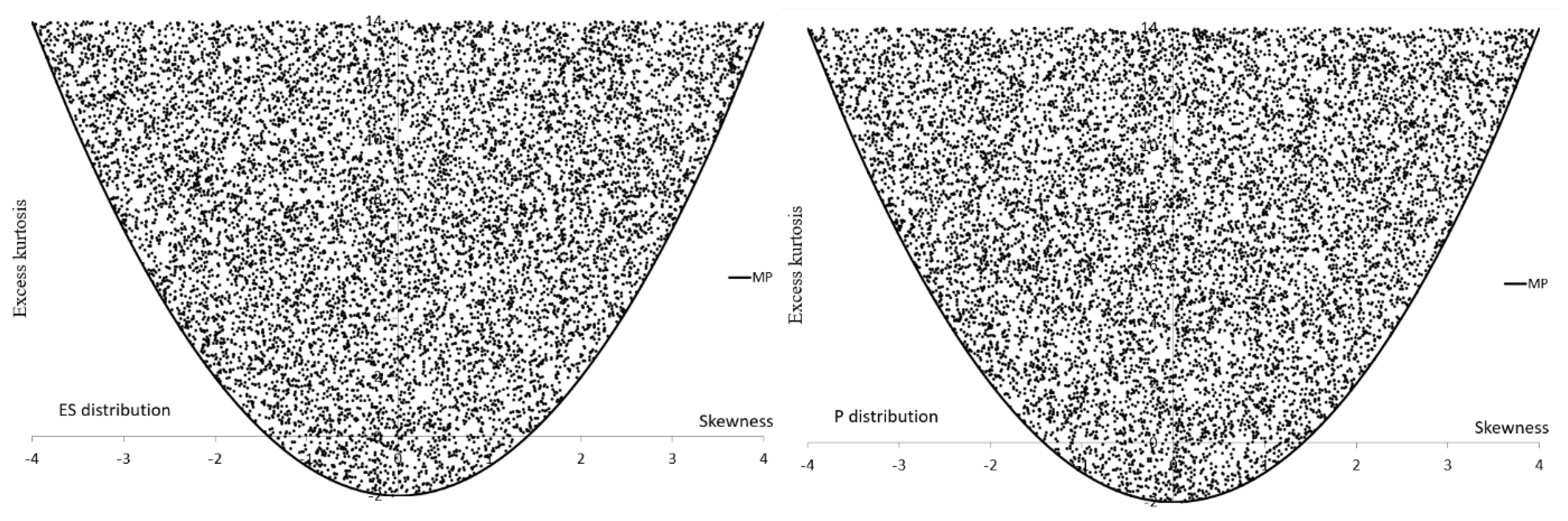
Figure 4.
A graphical range of and . The NM and NDPC distributions.
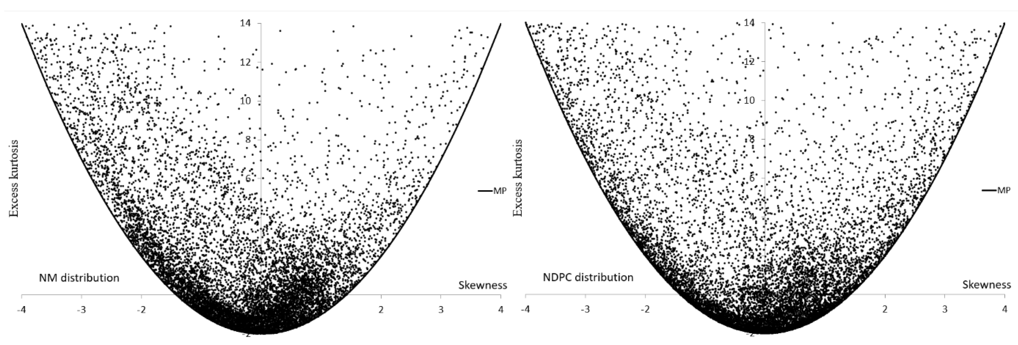
Table 1.
Articles devoted to normal GoFTs created in 21st century [16].
Table 1.
Articles devoted to normal GoFTs created in 21st century [16].
| Article | Sample sizes | Article | Sample sizes |
|---|---|---|---|
| Bonett and Seier [18] | 10,20,…,50,100 | Afeez et al. [19] |
10,30,50,100,300, 500,1000 |
| Aliaga et al. [20] | - | Marange and Qin [21] | 15, 30, 50, 80, 100, 150, 200 |
| Bontemps and Meddahi [22] | 100,250,500,1000 | Sulewski [23](2019) | 10,12,…,30,40,50 |
| Luceno [24] | 100 | Tavakoli et al. [25] |
5,6,…,15,20,25,30,40, 50,…,100 |
| Yazici and Yolacan [26] | 20,30,40,50 | Mishra et al. [27] | , |
| Gel et al. [28] | 20,50,100 | Kellner and Celisse [29] | 50,75,100,200,300,400 |
| Coin [30] | 20,50,200 | Wijekularathna et al. [31] |
5,10,20,30,50,75,100,200, 500,1000,2000 |
| Brys et al. [32] | 100,1000 | Sulewski [14] | 10,14,20 |
| Gel and Gastwirth [33] | 30,50,100 | Hernandez [34] | 5,10,…,30 |
| Romao et al. [35] | 25,50,100 | Khatun [36] |
10,20,25,30,40,50,100, 200,300 |
| Razali and Wah [37] |
20,30,50,100,200,…, 500,1000,2000 |
Arnastauskaitė et al. [38] | ,,…, |
| Noughabi and Arghami [39] | 10,20,30,50 | Bayoud [40] | 10,20,…,50,60,80,100 |
| Yap and Sim [41] |
10,20,30,50,100,300, 500,1000,2000 |
Uhm and Yi [42] | 10,20,30,100,200,300 |
| Chernobai et al. [43] | Sulewski [44] | 20,50,100 | |
| Ahmad and Khan [45] | 10,20,…,50,100,200,500 | Desgagné et al. [46] | 20,50,100,200 |
| Mbah and Paothong [47] |
10,20,30,50,100,200,…, 500,1000,2500,5000 |
Uyanto [48] | 10,30,50,70,100 |
| Torabi et al. [49] | 10,20,50,100,1000 | Ma et al. [50] | 10,30,50 |
| Feuerverger [51] | 200 | Giles [52] |
10,25,50,100,250, 500,1000 |
| Nosakhare and Bright [53] | 5,10,…,50,100 | Borrajo et al. [54] | 50,100,200,500 |
| Desgagné and Lafaye de Micheaux [55] | 10,12,…,20,50,100,200 | Terán-García and Pérez-Fernández [56] | 25,900 |
Table 2.
Groups of alternatives with signs (values) of and .
| Group | Group | ||||
|---|---|---|---|---|---|
| 0 | zero | zero | |||
| A | positive | positive | E | positive | negative |
| B | negative | positive | F | negative | negative |
| C | zero | positive | G | positive | zero |
| D | zero | negative | H | negative | zero |
Table 3.
A numerical range of and for alternatives in the MA .
| Alternative | Parameter ranges | ||
|---|---|---|---|
| ES | |||
| P | |||
| NM | |||
| NDPC | |||
| PCM | |||
| LM | |||
| SB | |||
| SU | |||
| EECK | 0 | ||
| EP | 0 |
Table 4.
SKS measure for alternatives in the MA for square side .
| Alternative | ||||
|---|---|---|---|---|
| ES | 0.9764 | 0.6733 | 0.4744 | 0.2507 |
| P | 0.9712 | 0.6791 | 0.4754 | 0.2524 |
| NM | 0.8874 | 0.3727 | 0.2779 | 0.1701 |
| NDPC | 0.9529 | 0.3845 | 0.2823 | 0.1677 |
| PCM | 0.9607 | 0.3644 | 0.2620 | 0.1546 |
| LM | 0.9005 | 0.3697 | 0.2770 | 0.1698 |
| SB | 0.4162 | 0.1052 | 0.0736 | 0.0432 |
| SU | 0.3953 | 0.0945 | 0.0687 | 0.0428 |
| EECK | 0 | 0 | 0 | 0 |
| EP | 0 | 0 | 0 | 0 |
Table 5.
Critical values (CVs) and test sizes (TSs) of analyzed GoFTs for sample sizes .
| No | GoFT | CV | TS | ||
|---|---|---|---|---|---|
| 1 | 0.2010 | 0.1622 | 0.049 | 0.050 | |
| 2 | 0.2417 | 0.1784 | 0.051 | 0.050 | |
| 3 | 0.2316 | 0.1748 | 0.051 | 0.049 | |
| 4 | 0.2419 | 0.1785 | 0.049 | 0.050 | |
| 5 | 0.2026 | 0.163 | 0.049 | 0.050 | |
| 6 | 0.2325 | 0.1746 | 0.051 | 0.050 | |
| 7 | 0.2268 | 0.173 | 0.050 | 0.049 | |
| 8 | 0.2327 | 0.1747 | 0.050 | 0.049 | |
| 9 | 0.2741 | 0.1971 | 0.052 | 0.050 | |
| 10 | 0.3413 | 0.2268 | 0.051 | 0.050 | |
| 11 | 0.3211 | 0.2133 | 0.051 | 0.050 | |
| 12 | 0.2619 | 0.192 | 0.050 | 0.050 | |
| 13 | 0.2769 | 0.1981 | 0.051 | 0.050 | |
| 14 | 0.3313 | 0.2218 | 0.051 | 0.050 | |
| 15 | 0.3141 | 0.211 | 0.051 | 0.050 | |
| 16 | 0.2635 | 0.1925 | 0.050 | 0.050 | |
| 17 | 0.1194 | 0.1232 | 0.050 | 0.050 | |
| 18 | 0.6867 | 0.7227 | 0.050 | 0.050 | |
| 19 | 0.8424 | 0.9034 | 0.050 | 0.051 | |
| 20 | 0.8445 | 0.9044 | 0.050 | 0.051 | |
Table 6.
The power of numbered tests (Ts) (see Table 5) for group A of alternatives (ALTs).
Table 6.
The power of numbered tests (Ts) (see Table 5) for group A of alternatives (ALTs).
| ALT/T | n | 19 | 20 | 18 | 17 | 3 | n | 19 | 20 | 18 | 17 | 3 |
|---|---|---|---|---|---|---|---|---|---|---|---|---|
| 10 | 0.285 | 0.254 | 0.248 | 0.234 | 0.220 | 20 | 0.570 | 0.502 | 0.473 | 0.419 | 0.371 | |
| 10 | 0.201 | 0.175 | 0.173 | 0.163 | 0.159 | 20 | 0.396 | 0.333 | 0.311 | 0.275 | 0.248 | |
| 10 | 0.134 | 0.117 | 0.115 | 0.108 | 0.110 | 20 | 0.242 | 0.200 | 0.179 | 0.159 | 0.149 | |
| ALT/T | n | 20 | 18 | 19 | 17 | 4 | n | 20 | 19 | 18 | 17 | 11 |
| 10 | 0.846 | 0.815 | 0.804 | 0.788 | 0.758 | 20 | 0.997 | 0.993 | 0.993 | 0.986 | 0.976 | |
| 10 | 0.846 | 0.812 | 0.804 | 0.783 | 0.754 | 20 | 0.997 | 0.993 | 0.993 | 0.986 | 0.977 | |
| 10 | 0.845 | 0.814 | 0.805 | 0.785 | 0.757 | 20 | 0.997 | 0.994 | 0.993 | 0.987 | 0.977 | |
| ALT/T | n | 4 | 8 | 19 | 20 | 18 | n | 4 | 8 | 19 | 20 | 18 |
| 10 | 0.135 | 0.133 | 0.111 | 0.104 | 0.103 | 20 | 0.199 | 0.193 | 0.194 | 0.188 | 0.171 | |
| 10 | 0.136 | 0.133 | 0.105 | 0.102 | 0.100 | 20 | 0.200 | 0.194 | 0.177 | 0.177 | 0.167 | |
| 10 | 0.082 | 0.081 | 0.066 | 0.064 | 0.064 | 20 | 0.098 | 0.094 | 0.085 | 0.081 | 0.079 | |
| ALT/T | n | 4 | 8 | 17 | 18 | 19 | n | 4 | 8 | 17 | 18 | 3 |
| 10 | 0.387 | 0.384 | 0.340 | 0.339 | 0.334 | 20 | 0.680 | 0.673 | 0.662 | 0.665 | 0.621 | |
| 10 | 0.180 | 0.178 | 0.133 | 0.129 | 0.119 | 20 | 0.299 | 0.292 | 0.244 | 0.227 | 0.222 | |
| 10 | 0.063 | 0.063 | 0.057 | 0.056 | 0.058 | 20 | 0.069 | 0.069 | 0.062 | 0.059 | 0.064 | |
| ALT/T | n | 20 | 4 | 8 | 18 | 17 | n | 20 | 18 | 19 | 4 | 17 |
| 10 | 0.594 | 0.549 | 0.550 | 0.589 | 0.578 | 20 | 0.896 | 0.895 | 0.863 | 0.831 | 0.871 | |
| 10 | 0.227 | 0.259 | 0.255 | 0.219 | 0.204 | 20 | 0.493 | 0.479 | 0.465 | 0.458 | 0.434 | |
| 10 | 0.067 | 0.079 | 0.078 | 0.064 | 0.062 | 20 | 0.094 | 0.082 | 0.097 | 0.098 | 0.076 | |
| ALT/T | n | 19 | 18 | 17 | 20 | 8 | n | 19 | 18 | 20 | 17 | 3 |
| 10 | 0.409 | 0.393 | 0.393 | 0.376 | 0.378 | 20 | 0.704 | 0.691 | 0.659 | 0.689 | 0.638 | |
| 10 | 0.174 | 0.152 | 0.148 | 0.154 | 0.143 | 20 | 0.316 | 0.267 | 0.272 | 0.250 | 0.230 | |
| 10 | 0.100 | 0.092 | 0.090 | 0.094 | 0.079 | 20 | 0.161 | 0.130 | 0.143 | 0.119 | 0.115 | |
| ALT/T | n | 4 | 8 | 20 | 19 | 18 | n | 4 | 8 | 20 | 19 | 18 |
| 10 | 0.117 | 0.115 | 0.089 | 0.087 | 0.084 | 20 | 0.172 | 0.166 | 0.165 | 0.152 | 0.143 | |
| 10 | 0.107 | 0.105 | 0.079 | 0.079 | 0.076 | 20 | 0.146 | 0.141 | 0.132 | 0.125 | 0.116 | |
| 10 | 0.096 | 0.095 | 0.071 | 0.071 | 0.069 | 20 | 0.127 | 0.122 | 0.112 | 0.108 | 0.100 | |
| ALT/T | n | 4 | 8 | 19 | 20 | 18 | n | 19 | 20 | 4 | 18 | 8 |
| 10 | 0.150 | 0.147 | 0.137 | 0.129 | 0.124 | 20 | 0.250 | 0.240 | 0.225 | 0.214 | 0.219 | |
| 10 | 0.100 | 0.100 | 0.100 | 0.091 | 0.089 | 20 | 0.165 | 0.146 | 0.135 | 0.131 | 0.132 | |
| 10 | 0.061 | 0.061 | 0.071 | 0.066 | 0.065 | 20 | 0.096 | 0.083 | 0.068 | 0.076 | 0.068 |
Table 7.
The power of numbered tests (Ts) (see Table 5) for group B of alternatives (ALTs).
Table 7.
The power of numbered tests (Ts) (see Table 5) for group B of alternatives (ALTs).
| ALT/T | n | 19 | 20 | 18 | 17 | 11 | n | 19 | 20 | 18 | 17 | 11 |
|---|---|---|---|---|---|---|---|---|---|---|---|---|
| 10 | 0.282 | 0.249 | 0.249 | 0.233 | 0.225 | 20 | 0.572 | 0.501 | 0.472 | 0.418 | 0.382 | |
| 10 | 0.202 | 0.177 | 0.174 | 0.163 | 0.163 | 20 | 0.394 | 0.331 | 0.306 | 0.270 | 0.258 | |
| 10 | 0.132 | 0.115 | 0.117 | 0.111 | 0.115 | 20 | 0.240 | 0.198 | 0.181 | 0.162 | 0.164 | |
| ALT/T | n | 20 | 18 | 19 | 17 | 9 | n | 20 | 19 | 18 | 17 | 9 |
| 10 | 0.846 | 0.815 | 0.804 | 0.787 | 0.780 | 20 | 0.997 | 0.994 | 0.993 | 0.986 | 0.970 | |
| 10 | 0.845 | 0.814 | 0.804 | 0.786 | 0.778 | 20 | 0.997 | 0.993 | 0.993 | 0.986 | 0.971 | |
| 10 | 0.847 | 0.813 | 0.806 | 0.784 | 0.777 | 20 | 0.997 | 0.994 | 0.993 | 0.987 | 0.970 | |
| ALT/T | n | 15 | 14 | 10 | 11 | 2 | n | 14 | 10 | 15 | 11 | 2 |
| 10 | 0.170 | 0.164 | 0.164 | 0.171 | 0.163 | 20 | 0.261 | 0.261 | 0.266 | 0.269 | 0.253 | |
| 10 | 0.141 | 0.143 | 0.143 | 0.141 | 0.142 | 20 | 0.223 | 0.223 | 0.215 | 0.214 | 0.214 | |
| 10 | 0.102 | 0.107 | 0.107 | 0.101 | 0.106 | 20 | 0.152 | 0.152 | 0.141 | 0.139 | 0.146 | |
| ALT/T | n | 15 | 11 | 14 | 10 | 2 | n | 19 | 20 | 18 | 11 | 15 |
| 10 | 0.682 | 0.678 | 0.689 | 0.689 | 0.689 | 20 | 0.950 | 0.949 | 0.960 | 0.952 | 0.952 | |
| 10 | 0.401 | 0.403 | 0.390 | 0.390 | 0.389 | 20 | 0.710 | 0.689 | 0.682 | 0.676 | 0.672 | |
| 10 | 0.165 | 0.166 | 0.157 | 0.157 | 0.156 | 20 | 0.302 | 0.282 | 0.247 | 0.260 | 0.257 | |
| ALT/T | n | 15 | 11 | 14 | 10 | 2 | n | 14 | 10 | 11 | 15 | 2 |
| 10 | 0.269 | 0.270 | 0.258 | 0.258 | 0.257 | 20 | 0.454 | 0.454 | 0.464 | 0.461 | 0.444 | |
| 10 | 0.237 | 0.234 | 0.243 | 0.243 | 0.242 | 20 | 0.431 | 0.431 | 0.416 | 0.418 | 0.421 | |
| 10 | 0.060 | 0.061 | 0.060 | 0.060 | 0.060 | 20 | 0.068 | 0.068 | 0.068 | 0.068 | 0.067 | |
| ALT/T | n | 19 | 20 | 18 | 17 | 11 | n | 19 | 20 | 18 | 17 | 11 |
| 10 | 0.202 | 0.189 | 0.186 | 0.179 | 0.180 | 20 | 0.377 | 0.340 | 0.338 | 0.312 | 0.293 | |
| 10 | 0.167 | 0.148 | 0.146 | 0.141 | 0.141 | 20 | 0.305 | 0.260 | 0.247 | 0.227 | 0.217 | |
| 10 | 0.162 | 0.140 | 0.144 | 0.142 | 0.131 | 20 | 0.284 | 0.237 | 0.239 | 0.230 | 0.204 | |
| ALT/T | n | 14 | 10 | 2 | 15 | 6 | n | 14 | 10 | 2 | 20 | 13 |
| 10 | 0.167 | 0.167 | 0.166 | 0.165 | 0.163 | 20 | 0.274 | 0.274 | 0.263 | 0.293 | 0.260 | |
| 10 | 0.111 | 0.111 | 0.110 | 0.108 | 0.108 | 20 | 0.158 | 0.158 | 0.151 | 0.140 | 0.150 | |
| 10 | 0.097 | 0.097 | 0.096 | 0.094 | 0.094 | 20 | 0.130 | 0.130 | 0.123 | 0.104 | 0.123 | |
| ALT/T | n | 15 | 11 | 14 | 10 | 2 | n | 14 | 10 | 11 | 15 | 2 |
| 10 | 0.130 | 0.130 | 0.130 | 0.130 | 0.129 | 20 | 0.192 | 0.192 | 0.189 | 0.188 | 0.184 | |
| 10 | 0.112 | 0.112 | 0.112 | 0.112 | 0.111 | 20 | 0.156 | 0.156 | 0.152 | 0.152 | 0.149 | |
| 10 | 0.070 | 0.070 | 0.068 | 0.068 | 0.068 | 20 | 0.078 | 0.078 | 0.077 | 0.077 | 0.075 |
Table 8.
The power of numbered tests (Ts) (see Table 5) for group C of alternatives (ALTs).
Table 8.
The power of numbered tests (Ts) (see Table 5) for group C of alternatives (ALTs).
| ALT/T | n | 19 | 20 | 18 | 17 | 3 | n | 19 | 20 | 18 | 17 | 3 |
|---|---|---|---|---|---|---|---|---|---|---|---|---|
| 10 | 0.284 | 0.249 | 0.245 | 0.230 | 0.220 | 20 | 0.571 | 0.495 | 0.470 | 0.413 | 0.366 | |
| 10 | 0.201 | 0.174 | 0.173 | 0.161 | 0.159 | 20 | 0.397 | 0.330 | 0.308 | 0.272 | 0.245 | |
| 10 | 0.135 | 0.117 | 0.116 | 0.109 | 0.111 | 20 | 0.240 | 0.196 | 0.179 | 0.159 | 0.149 | |
| ALT/T | n | 19 | 18 | 20 | 3 | 17 | n | 19 | 20 | 18 | 17 | 3 |
| 10 | 0.137 | 0.124 | 0.121 | 0.119 | 0.119 | 20 | 0.243 | 0.209 | 0.193 | 0.178 | 0.169 | |
| 10 | 0.137 | 0.123 | 0.122 | 0.119 | 0.117 | 20 | 0.242 | 0.210 | 0.190 | 0.174 | 0.166 | |
| 10 | 0.138 | 0.120 | 0.122 | 0.116 | 0.115 | 20 | 0.240 | 0.206 | 0.190 | 0.174 | 0.166 | |
| ALT/T | n | 3 | 7 | 19 | 17 | 18 | n | 17 | 3 | 7 | 18 | 19 |
| 10 | 0.222 | 0.219 | 0.204 | 0.216 | 0.202 | 20 | 0.391 | 0.387 | 0.380 | 0.357 | 0.325 | |
| 10 | 0.138 | 0.135 | 0.135 | 0.130 | 0.127 | 20 | 0.214 | 0.213 | 0.208 | 0.203 | 0.205 | |
| 10 | 0.064 | 0.064 | 0.072 | 0.063 | 0.064 | 20 | 0.070 | 0.072 | 0.070 | 0.075 | 0.095 | |
| ALT/T | n | 3 | 17 | 7 | 18 | 19 | n | 17 | 3 | 18 | 7 | 11 |
| 10 | 0.181 | 0.179 | 0.178 | 0.169 | 0.166 | 20 | 0.318 | 0.302 | 0.292 | 0.295 | 0.279 | |
| 10 | 0.059 | 0.059 | 0.059 | 0.060 | 0.064 | 20 | 0.063 | 0.064 | 0.065 | 0.064 | 0.062 | |
| 10 | 0.052 | 0.053 | 0.052 | 0.054 | 0.052 | 20 | 0.052 | 0.051 | 0.054 | 0.051 | 0.050 | |
| ALT/T | n | 3 | 7 | 19 | 11 | 17 | n | 3 | 7 | 11 | 17 | 15 |
| 10 | 0.085 | 0.083 | 0.093 | 0.082 | 0.082 | 20 | 0.108 | 0.105 | 0.104 | 0.109 | 0.101 | |
| 10 | 0.119 | 0.117 | 0.103 | 0.107 | 0.108 | 20 | 0.175 | 0.172 | 0.161 | 0.159 | 0.158 | |
| 10 | 0.084 | 0.082 | 0.079 | 0.079 | 0.077 | 20 | 0.106 | 0.104 | 0.102 | 0.097 | 0.099 | |
| ALT/T | n | 19 | 18 | 3 | 17 | 7 | n | 19 | 18 | 20 | 17 | 3 |
| 10 | 0.177 | 0.159 | 0.159 | 0.157 | 0.156 | 20 | 0.312 | 0.271 | 0.260 | 0.265 | 0.253 | |
| 10 | 0.170 | 0.152 | 0.151 | 0.150 | 0.148 | 20 | 0.300 | 0.257 | 0.251 | 0.249 | 0.238 | |
| 10 | 0.164 | 0.146 | 0.145 | 0.142 | 0.141 | 20 | 0.290 | 0.242 | 0.240 | 0.232 | 0.221 | |
| ALT/T | n | 18 | 17 | 11 | 13 | 19 | n | 18 | 17 | 1 | 2 | 6 |
| 10 | 0.050 | 0.050 | 0.051 | 0.051 | 0.050 | 20 | 0.050 | 0.049 | 0.049 | 0.049 | 0.049 | |
| 10 | 0.051 | 0.051 | 0.051 | 0.050 | 0.051 | 20 | 0.051 | 0.051 | 0.050 | 0.051 | 0.051 | |
| 10 | 0.051 | 0.051 | 0.050 | 0.050 | 0.050 | 20 | 0.050 | 0.050 | 0.051 | 0.050 | 0.050 | |
| ALT/T | n | 19 | 20 | 18 | 3 | 7 | n | 19 | 20 | 18 | 17 | 3 |
| 10 | 0.104 | 0.093 | 0.091 | 0.090 | 0.088 | 20 | 0.169 | 0.144 | 0.131 | 0.120 | 0.115 | |
| 10 | 0.106 | 0.094 | 0.092 | 0.091 | 0.089 | 20 | 0.169 | 0.143 | 0.130 | 0.120 | 0.116 | |
| 10 | 0.063 | 0.059 | 0.058 | 0.059 | 0.059 | 20 | 0.079 | 0.071 | 0.065 | 0.063 | 0.063 | |
| ALT/T | n | 19 | 3 | 7 | 18 | 17 | n | 19 | 18 | 20 | 17 | 3 |
| 10 | 0.155 | 0.140 | 0.137 | 0.137 | 0.135 | 20 | 0.263 | 0.223 | 0.217 | 0.217 | 0.210 | |
| 10 | 0.091 | 0.084 | 0.082 | 0.082 | 0.080 | 20 | 0.134 | 0.107 | 0.111 | 0.103 | 0.104 | |
| 10 | 0.096 | 0.088 | 0.086 | 0.085 | 0.084 | 20 | 0.141 | 0.116 | 0.116 | 0.113 | 0.115 | |
| ALT/T | n | 19 | 3 | 7 | 18 | 11 | n | 19 | 20 | 3 | 18 | 7 |
| 10 | 0.072 | 0.067 | 0.066 | 0.065 | 0.065 | 20 | 0.093 | 0.079 | 0.076 | 0.076 | 0.074 | |
| 10 | 0.066 | 0.063 | 0.062 | 0.060 | 0.060 | 20 | 0.079 | 0.069 | 0.067 | 0.066 | 0.066 | |
| 10 | 0.060 | 0.057 | 0.056 | 0.057 | 0.057 | 20 | 0.069 | 0.062 | 0.060 | 0.059 | 0.059 |
Table 9.
The power of numbered tests (Ts) (see Table 5) for group D of alternatives (ALTs).
Table 9.
The power of numbered tests (Ts) (see Table 5) for group D of alternatives (ALTs).
| ALT/T | n | 20 | 18 | 17 | 19 | 1 | n | 20 | 18 | 19 | 17 | 1 |
|---|---|---|---|---|---|---|---|---|---|---|---|---|
| 10 | 0.667 | 0.601 | 0.528 | 0.481 | 0.481 | 20 | 0.981 | 0.949 | 0.917 | 0.888 | 0.802 | |
| 10 | 0.666 | 0.598 | 0.524 | 0.483 | 0.480 | 20 | 0.981 | 0.949 | 0.919 | 0.888 | 0.801 | |
| 10 | 0.664 | 0.597 | 0.523 | 0.483 | 0.477 | 20 | 0.980 | 0.951 | 0.918 | 0.890 | 0.804 | |
| ALT/T | n | 9 | 1 | 13 | 5 | 20 | n | 18 | 9 | 20 | 13 | 1 |
| 10 | 0.199 | 0.208 | 0.189 | 0.199 | 0.184 | 20 | 0.471 | 0.416 | 0.413 | 0.402 | 0.426 | |
| 10 | 0.237 | 0.218 | 0.218 | 0.206 | 0.213 | 20 | 0.432 | 0.470 | 0.479 | 0.448 | 0.413 | |
| 10 | 0.055 | 0.058 | 0.053 | 0.056 | 0.047 | 20 | 0.060 | 0.064 | 0.054 | 0.062 | 0.071 | |
| ALT/T | n | 1 | 9 | 5 | 13 | 17 | n | 1 | 17 | 5 | 9 | 18 |
| 10 | 0.126 | 0.119 | 0.120 | 0.114 | 0.111 | 20 | 0.227 | 0.237 | 0.219 | 0.212 | 0.231 | |
| 10 | 0.063 | 0.064 | 0.062 | 0.062 | 0.052 | 20 | 0.084 | 0.070 | 0.081 | 0.082 | 0.066 | |
| 10 | 0.049 | 0.049 | 0.049 | 0.050 | 0.047 | 20 | 0.049 | 0.046 | 0.048 | 0.049 | 0.045 | |
| ALT/T | n | 9 | 1 | 13 | 5 | 2 | n | 1 | 9 | 5 | 13 | 4 |
| 10 | 0.049 | 0.049 | 0.049 | 0.048 | 0.048 | 20 | 0.050 | 0.049 | 0.049 | 0.049 | 0.049 | |
| 10 | 0.061 | 0.061 | 0.059 | 0.060 | 0.054 | 20 | 0.077 | 0.076 | 0.075 | 0.074 | 0.066 | |
| 10 | 0.050 | 0.050 | 0.050 | 0.049 | 0.048 | 20 | 0.053 | 0.052 | 0.052 | 0.051 | 0.049 | |
| ALT/T | n | 1 | 18 | 5 | 17 | 20 | n | 18 | 17 | 1 | 5 | 20 |
| 10 | 0.215 | 0.197 | 0.208 | 0.201 | 0.177 | 20 | 0.422 | 0.432 | 0.412 | 0.401 | 0.341 | |
| 10 | 0.270 | 0.270 | 0.260 | 0.260 | 0.250 | 20 | 0.572 | 0.539 | 0.514 | 0.502 | 0.507 | |
| 10 | 0.213 | 0.224 | 0.205 | 0.206 | 0.212 | 20 | 0.458 | 0.396 | 0.384 | 0.374 | 0.424 | |
| ALT/T | n | 1 | 9 | 5 | 13 | 4 | n | 9 | 13 | 1 | 5 | 14 |
| 10 | 0.049 | 0.049 | 0.048 | 0.049 | 0.048 | 20 | 0.048 | 0.048 | 0.048 | 0.047 | 0.047 | |
| 10 | 0.049 | 0.049 | 0.049 | 0.049 | 0.049 | 20 | 0.051 | 0.051 | 0.050 | 0.049 | 0.050 | |
| 10 | 0.051 | 0.050 | 0.050 | 0.049 | 0.049 | 20 | 0.048 | 0.048 | 0.048 | 0.048 | 0.047 | |
| ALT/T | n | 11 | 15 | 9 | 12 | 18 | n | 15 | 11 | 14 | 2 | 10 |
| 10 | 0.052 | 0.051 | 0.051 | 0.052 | 0.052 | 20 | 0.050 | 0.050 | 0.050 | 0.050 | 0.050 | |
| 10 | 0.052 | 0.052 | 0.051 | 0.051 | 0.051 | 20 | 0.051 | 0.051 | 0.051 | 0.051 | 0.051 | |
| 10 | 0.051 | 0.051 | 0.051 | 0.051 | 0.051 | 20 | 0.050 | 0.050 | 0.050 | 0.050 | 0.050 | |
| ALT/T | n | 9 | 1 | 13 | 5 | 14 | n | 9 | 1 | 13 | 5 | 18 |
| 10 | 0.065 | 0.063 | 0.062 | 0.060 | 0.052 | 20 | 0.086 | 0.085 | 0.082 | 0.080 | 0.078 | |
| 10 | 0.053 | 0.052 | 0.052 | 0.051 | 0.048 | 20 | 0.057 | 0.055 | 0.055 | 0.053 | 0.046 | |
| 10 | 0.050 | 0.049 | 0.050 | 0.049 | 0.047 | 20 | 0.051 | 0.050 | 0.050 | 0.049 | 0.044 | |
| ALT/T | n | 9 | 1 | 13 | 5 | 18 | n | 20 | 18 | 9 | 1 | 13 |
| 10 | 0.083 | 0.081 | 0.078 | 0.077 | 0.074 | 20 | 0.188 | 0.163 | 0.130 | 0.129 | 0.124 | |
| 10 | 0.059 | 0.058 | 0.057 | 0.056 | 0.047 | 20 | 0.056 | 0.061 | 0.072 | 0.070 | 0.069 | |
| 10 | 0.055 | 0.054 | 0.053 | 0.053 | 0.045 | 20 | 0.045 | 0.050 | 0.061 | 0.060 | 0.059 |
Table 10.
The power of numbered tests (Ts) (see Table 5) for group E of alternatives (ALTs).
Table 10.
The power of numbered tests (Ts) (see Table 5) for group E of alternatives (ALTs).
| ALT/T | n | 20 | 18 | 17 | 4 | 19 | n | 20 | 18 | 19 | 17 | 4 |
|---|---|---|---|---|---|---|---|---|---|---|---|---|
| 10 | 0.775 | 0.740 | 0.701 | 0.684 | 0.685 | 20 | 0.990 | 0.979 | 0.970 | 0.961 | 0.936 | |
| 10 | 0.778 | 0.741 | 0.703 | 0.687 | 0.685 | 20 | 0.991 | 0.979 | 0.970 | 0.960 | 0.935 | |
| 10 | 0.776 | 0.741 | 0.704 | 0.688 | 0.686 | 20 | 0.991 | 0.980 | 0.970 | 0.962 | 0.937 | |
| ALT/T | n | 4 | 8 | 18 | 17 | 20 | n | 4 | 8 | 18 | 17 | 20 |
| 10 | 0.137 | 0.135 | 0.093 | 0.092 | 0.089 | 20 | 0.212 | 0.205 | 0.166 | 0.163 | 0.157 | |
| 10 | 0.093 | 0.091 | 0.064 | 0.065 | 0.063 | 20 | 0.122 | 0.117 | 0.087 | 0.087 | 0.086 | |
| 10 | 0.065 | 0.064 | 0.053 | 0.053 | 0.051 | 20 | 0.071 | 0.070 | 0.057 | 0.056 | 0.052 | |
| ALT/T | n | 4 | 8 | 17 | 18 | 1 | n | 4 | 8 | 17 | 18 | 1 |
| 10 | 0.693 | 0.689 | 0.659 | 0.645 | 0.628 | 20 | 0.963 | 0.962 | 0.974 | 0.969 | 0.951 | |
| 10 | 0.107 | 0.105 | 0.072 | 0.073 | 0.077 | 20 | 0.165 | 0.159 | 0.127 | 0.127 | 0.124 | |
| 10 | 0.081 | 0.079 | 0.058 | 0.056 | 0.062 | 20 | 0.102 | 0.099 | 0.075 | 0.073 | 0.077 | |
| ALT/T | n | 4 | 8 | 1 | 5 | 18 | n | 4 | 8 | 1 | 18 | 5 |
| 10 | 0.153 | 0.151 | 0.130 | 0.125 | 0.116 | 20 | 0.278 | 0.270 | 0.244 | 0.244 | 0.236 | |
| 10 | 0.087 | 0.086 | 0.076 | 0.074 | 0.066 | 20 | 0.135 | 0.131 | 0.120 | 0.109 | 0.117 | |
| 10 | 0.073 | 0.071 | 0.056 | 0.055 | 0.051 | 20 | 0.090 | 0.087 | 0.067 | 0.069 | 0.065 | |
| ALT/T | n | 1 | 4 | 8 | 5 | 18 | n | 1 | 4 | 8 | 5 | 18 |
| 10 | 0.864 | 0.874 | 0.873 | 0.859 | 0.873 | 20 | 0.997 | 0.997 | 0.997 | 0.997 | 0.998 | |
| 10 | 0.434 | 0.411 | 0.409 | 0.417 | 0.395 | 20 | 0.741 | 0.732 | 0.728 | 0.728 | 0.739 | |
| 10 | 0.125 | 0.129 | 0.128 | 0.122 | 0.109 | 20 | 0.211 | 0.215 | 0.213 | 0.206 | 0.191 | |
| ALT/T | n | 20 | 4 | 8 | 18 | 17 | n | 20 | 18 | 19 | 17 | 4 |
| 10 | 0.495 | 0.442 | 0.437 | 0.458 | 0.427 | 20 | 0.892 | 0.844 | 0.799 | 0.791 | 0.746 | |
| 10 | 0.213 | 0.232 | 0.229 | 0.197 | 0.186 | 20 | 0.502 | 0.441 | 0.401 | 0.394 | 0.410 | |
| 10 | 0.048 | 0.063 | 0.062 | 0.048 | 0.048 | 20 | 0.049 | 0.051 | 0.042 | 0.051 | 0.069 | |
| ALT/T | n | 4 | 8 | 1 | 5 | 12 | n | 4 | 19 | 8 | 20 | 18 |
| 10 | 0.052 | 0.052 | 0.050 | 0.050 | 0.049 | 20 | 0.052 | 0.052 | 0.052 | 0.051 | 0.050 | |
| 10 | 0.051 | 0.051 | 0.051 | 0.051 | 0.051 | 20 | 0.049 | 0.050 | 0.049 | 0.050 | 0.050 | |
| 10 | 0.050 | 0.051 | 0.052 | 0.052 | 0.051 | 20 | 0.049 | 0.049 | 0.049 | 0.049 | 0.048 |
Table 11.
The power of numbered tests (Ts) (see Table 5) for group F of alternatives (ALTs).
Table 11.
The power of numbered tests (Ts) (see Table 5) for group F of alternatives (ALTs).
| ALT/T | n | 20 | 18 | 9 | 13 | 17 | n | 20 | 18 | 19 | 17 | 9 |
|---|---|---|---|---|---|---|---|---|---|---|---|---|
| 10 | 0.778 | 0.738 | 0.735 | 0.726 | 0.701 | 20 | 0.990 | 0.980 | 0.969 | 0.961 | 0.953 | |
| 10 | 0.777 | 0.741 | 0.736 | 0.727 | 0.703 | 20 | 0.990 | 0.980 | 0.970 | 0.962 | 0.954 | |
| 10 | 0.778 | 0.739 | 0.735 | 0.726 | 0.701 | 20 | 0.990 | 0.979 | 0.969 | 0.961 | 0.954 | |
| ALT/T | n | 9 | 13 | 14 | 10 | 2 | n | 9 | 13 | 14 | 10 | 2 |
| 10 | 0.322 | 0.321 | 0.312 | 0.312 | 0.310 | 20 | 0.597 | 0.595 | 0.589 | 0.589 | 0.577 | |
| 10 | 0.105 | 0.101 | 0.089 | 0.089 | 0.089 | 20 | 0.152 | 0.147 | 0.132 | 0.132 | 0.127 | |
| 10 | 0.056 | 0.056 | 0.057 | 0.057 | 0.057 | 20 | 0.058 | 0.058 | 0.060 | 0.060 | 0.059 | |
| ALT/T | n | 13 | 9 | 14 | 10 | 2 | n | 9 | 14 | 10 | 13 | 2 |
| 10 | 0.295 | 0.295 | 0.289 | 0.289 | 0.287 | 20 | 0.550 | 0.549 | 0.549 | 0.549 | 0.536 | |
| 10 | 0.101 | 0.102 | 0.099 | 0.099 | 0.098 | 20 | 0.145 | 0.144 | 0.144 | 0.144 | 0.137 | |
| 10 | 0.054 | 0.054 | 0.053 | 0.053 | 0.053 | 20 | 0.055 | 0.056 | 0.055 | 0.056 | 0.054 | |
| ALT/T | n | 9 | 13 | 14 | 10 | 2 | n | 20 | 18 | 9 | 13 | 17 |
| 10 | 0.143 | 0.141 | 0.130 | 0.130 | 0.130 | 20 | 0.340 | 0.318 | 0.253 | 0.249 | 0.269 | |
| 10 | 0.067 | 0.064 | 0.058 | 0.058 | 0.058 | 20 | 0.063 | 0.067 | 0.084 | 0.080 | 0.066 | |
| 10 | 0.051 | 0.050 | 0.048 | 0.048 | 0.048 | 20 | 0.041 | 0.044 | 0.052 | 0.051 | 0.045 | |
| ALT/T | n | 9 | 13 | 18 | 17 | 6 | n | 18 | 17 | 9 | 13 | 1 |
| 10 | 0.276 | 0.277 | 0.299 | 0.287 | 0.275 | 20 | 0.624 | 0.589 | 0.520 | 0.519 | 0.529 | |
| 10 | 0.234 | 0.236 | 0.225 | 0.224 | 0.237 | 20 | 0.475 | 0.464 | 0.429 | 0.430 | 0.397 | |
| 10 | 0.131 | 0.127 | 0.112 | 0.115 | 0.111 | 20 | 0.204 | 0.216 | 0.226 | 0.220 | 0.229 | |
| ALT/T | n | 9 | 13 | 14 | 10 | 2 | n | 20 | 9 | 13 | 14 | 10 |
| 10 | 0.524 | 0.518 | 0.488 | 0.488 | 0.485 | 20 | 0.916 | 0.814 | 0.808 | 0.792 | 0.792 | |
| 10 | 0.129 | 0.129 | 0.126 | 0.126 | 0.125 | 20 | 0.181 | 0.200 | 0.200 | 0.202 | 0.202 | |
| 10 | 0.106 | 0.106 | 0.106 | 0.106 | 0.105 | 20 | 0.123 | 0.149 | 0.149 | 0.153 | 0.153 | |
| ALT/T | n | 11 | 15 | 14 | 10 | 2 | n | 11 | 14 | 10 | 15 | 19 |
| 10 | 0.051 | 0.051 | 0.051 | 0.051 | 0.051 | 20 | 0.051 | 0.052 | 0.051 | 0.051 | 0.051 | |
| 10 | 0.067 | 0.066 | 0.065 | 0.065 | 0.065 | 20 | 0.078 | 0.077 | 0.077 | 0.076 | 0.078 | |
| 10 | 0.052 | 0.052 | 0.051 | 0.051 | 0.051 | 20 | 0.054 | 0.054 | 0.054 | 0.054 | 0.050 |
Table 12.
The power of numbered tests (Ts) (see Table 5) for group G of alternatives (ALTs).
Table 12.
The power of numbered tests (Ts) (see Table 5) for group G of alternatives (ALTs).
| ALT/T | n | 20 | 18 | 17 | 19 | 4 | n | 20 | 18 | 19 | 17 | 4 |
|---|---|---|---|---|---|---|---|---|---|---|---|---|
| 10 | 0.801 | 0.767 | 0.733 | 0.727 | 0.715 | 20 | 0.992 | 0.985 | 0.978 | 0.971 | 0.950 | |
| 10 | 0.800 | 0.765 | 0.732 | 0.727 | 0.716 | 20 | 0.992 | 0.985 | 0.978 | 0.971 | 0.949 | |
| 10 | 0.801 | 0.766 | 0.733 | 0.726 | 0.715 | 20 | 0.993 | 0.984 | 0.978 | 0.970 | 0.950 | |
| ALT/T | n | 4 | 8 | 18 | 17 | 20 | n | 4 | 8 | 20 | 18 | 19 |
| 10 | 0.095 | 0.094 | 0.066 | 0.065 | 0.066 | 20 | 0.124 | 0.119 | 0.094 | 0.091 | 0.087 | |
| 10 | 0.063 | 0.062 | 0.052 | 0.052 | 0.051 | 20 | 0.067 | 0.066 | 0.056 | 0.054 | 0.056 | |
| 10 | 0.057 | 0.057 | 0.051 | 0.051 | 0.050 | 20 | 0.061 | 0.060 | 0.052 | 0.051 | 0.052 | |
| ALT/T | n | 4 | 8 | 1 | 5 | 18 | n | 4 | 8 | 18 | 20 | 1 |
| 10 | 0.174 | 0.172 | 0.128 | 0.127 | 0.122 | 20 | 0.304 | 0.296 | 0.238 | 0.244 | 0.237 | |
| 10 | 0.095 | 0.095 | 0.104 | 0.101 | 0.094 | 20 | 0.155 | 0.155 | 0.168 | 0.164 | 0.170 | |
| 10 | 0.095 | 0.094 | 0.065 | 0.065 | 0.068 | 20 | 0.131 | 0.126 | 0.094 | 0.088 | 0.087 | |
| ALT/T | n | 4 | 8 | 1 | 5 | 18 | n | 4 | 8 | 18 | 17 | 1 |
| 10 | 0.273 | 0.270 | 0.208 | 0.207 | 0.206 | 20 | 0.514 | 0.504 | 0.407 | 0.403 | 0.405 | |
| 10 | 0.137 | 0.137 | 0.139 | 0.135 | 0.130 | 20 | 0.241 | 0.239 | 0.258 | 0.250 | 0.244 | |
| 10 | 0.086 | 0.084 | 0.061 | 0.061 | 0.063 | 20 | 0.105 | 0.101 | 0.080 | 0.074 | 0.072 | |
| ALT/T | n | 4 | 8 | 17 | 18 | 1 | n | 17 | 4 | 8 | 18 | 1 |
| 10 | 0.573 | 0.569 | 0.518 | 0.512 | 0.517 | 20 | 0.870 | 0.881 | 0.877 | 0.868 | 0.859 | |
| 10 | 0.513 | 0.509 | 0.456 | 0.448 | 0.422 | 20 | 0.834 | 0.835 | 0.830 | 0.820 | 0.778 | |
| 10 | 0.089 | 0.090 | 0.102 | 0.100 | 0.117 | 20 | 0.172 | 0.143 | 0.147 | 0.165 | 0.186 | |
| ALT/T | n | 4 | 8 | 20 | 18 | 17 | n | 4 | 8 | 20 | 18 | 19 |
| 10 | 0.090 | 0.089 | 0.064 | 0.062 | 0.061 | 20 | 0.117 | 0.113 | 0.096 | 0.087 | 0.087 | |
| 10 | 0.083 | 0.081 | 0.059 | 0.059 | 0.058 | 20 | 0.103 | 0.099 | 0.084 | 0.077 | 0.077 | |
| 10 | 0.068 | 0.067 | 0.053 | 0.053 | 0.053 | 20 | 0.077 | 0.074 | 0.061 | 0.058 | 0.059 | |
| ALT/T | n | 4 | 8 | 19 | 17 | 5 | n | 4 | 8 | 19 | 20 | 18 |
| 10 | 0.064 | 0.063 | 0.054 | 0.053 | 0.053 | 20 | 0.071 | 0.069 | 0.060 | 0.060 | 0.057 | |
| 10 | 0.059 | 0.059 | 0.051 | 0.051 | 0.051 | 20 | 0.066 | 0.064 | 0.054 | 0.055 | 0.053 | |
| 10 | 0.050 | 0.050 | 0.050 | 0.050 | 0.050 | 20 | 0.050 | 0.050 | 0.050 | 0.049 | 0.049 |
Table 13.
The power of numbered tests (Ts) (see Table 5) for group H of alternatives (ALTs).
Table 13.
The power of numbered tests (Ts) (see Table 5) for group H of alternatives (ALTs).
| ALT/T | n | 20 | 18 | 9 | 13 | 17 | n | 20 | 18 | 19 | 17 | 9 |
|---|---|---|---|---|---|---|---|---|---|---|---|---|
| 10 | 0.801 | 0.764 | 0.757 | 0.750 | 0.732 | 20 | 0.992 | 0.984 | 0.978 | 0.971 | 0.963 | |
| 10 | 0.801 | 0.766 | 0.759 | 0.752 | 0.731 | 20 | 0.993 | 0.984 | 0.979 | 0.970 | 0.962 | |
| 10 | 0.800 | 0.767 | 0.757 | 0.751 | 0.735 | 20 | 0.993 | 0.985 | 0.979 | 0.971 | 0.962 | |
| ALT/T | n | 14 | 10 | 2 | 13 | 6 | n | 14 | 10 | 2 | 13 | 9 |
| 10 | 0.118 | 0.118 | 0.117 | 0.115 | 0.114 | 20 | 0.175 | 0.175 | 0.167 | 0.168 | 0.168 | |
| 10 | 0.098 | 0.098 | 0.097 | 0.095 | 0.095 | 20 | 0.131 | 0.131 | 0.125 | 0.123 | 0.123 | |
| 10 | 0.058 | 0.058 | 0.058 | 0.058 | 0.058 | 20 | 0.063 | 0.063 | 0.061 | 0.060 | 0.060 | |
| ALT/T | n | 14 | 10 | 2 | 13 | 15 | n | 14 | 10 | 2 | 13 | 15 |
| 10 | 0.165 | 0.165 | 0.164 | 0.157 | 0.163 | 20 | 0.280 | 0.280 | 0.269 | 0.264 | 0.269 | |
| 10 | 0.095 | 0.095 | 0.094 | 0.096 | 0.092 | 20 | 0.131 | 0.131 | 0.124 | 0.126 | 0.122 | |
| 10 | 0.055 | 0.055 | 0.055 | 0.057 | 0.054 | 20 | 0.060 | 0.060 | 0.058 | 0.059 | 0.057 | |
| ALT/T | n | 14 | 10 | 2 | 13 | 9 | n | 14 | 10 | 2 | 13 | 9 |
| 10 | 0.080 | 0.080 | 0.079 | 0.078 | 0.078 | 20 | 0.101 | 0.101 | 0.097 | 0.096 | 0.095 | |
| 10 | 0.063 | 0.063 | 0.063 | 0.063 | 0.063 | 20 | 0.071 | 0.071 | 0.069 | 0.069 | 0.069 | |
| 10 | 0.074 | 0.074 | 0.074 | 0.074 | 0.074 | 20 | 0.092 | 0.092 | 0.088 | 0.088 | 0.088 | |
| ALT/T | n | 18 | 17 | 20 | 13 | 6 | n | 18 | 17 | 20 | 9 | 13 |
| 10 | 0.387 | 0.361 | 0.373 | 0.348 | 0.366 | 20 | 0.744 | 0.693 | 0.707 | 0.632 | 0.638 | |
| 10 | 0.128 | 0.132 | 0.117 | 0.166 | 0.159 | 20 | 0.239 | 0.252 | 0.193 | 0.278 | 0.277 | |
| 10 | 0.133 | 0.135 | 0.122 | 0.092 | 0.080 | 20 | 0.256 | 0.260 | 0.206 | 0.188 | 0.181 | |
| ALT/T | n | 14 | 10 | 2 | 13 | 9 | n | 14 | 10 | 9 | 13 | 2 |
| 10 | 0.110 | 0.110 | 0.109 | 0.110 | 0.110 | 20 | 0.165 | 0.165 | 0.160 | 0.160 | 0.157 | |
| 10 | 0.079 | 0.079 | 0.078 | 0.077 | 0.077 | 20 | 0.099 | 0.099 | 0.094 | 0.095 | 0.094 | |
| 10 | 0.079 | 0.079 | 0.078 | 0.077 | 0.076 | 20 | 0.099 | 0.099 | 0.095 | 0.094 | 0.094 | |
| ALT/T | n | 11 | 14 | 10 | 2 | 15 | n | 14 | 10 | 11 | 15 | 2 |
| 10 | 0.051 | 0.051 | 0.051 | 0.051 | 0.051 | 20 | 0.051 | 0.051 | 0.051 | 0.051 | 0.050 | |
| 10 | 0.060 | 0.060 | 0.060 | 0.060 | 0.060 | 20 | 0.068 | 0.067 | 0.066 | 0.066 | 0.066 | |
| 10 | 0.058 | 0.058 | 0.058 | 0.058 | 0.058 | 20 | 0.062 | 0.062 | 0.061 | 0.061 | 0.060 |
Table 14.
Real data examples with sources, sample size, and values.
| Ex | Description | Source | n | ||
|---|---|---|---|---|---|
| I | Socio-economic data (percentage of draftees receiving highest mark on army examination) for 47 French-speaking provinces of Switzerland. | R package swiss[3] | 47 | ||
| II | The data give the distances taken to stop. | cars[2] | 50 | 0.782 | 0.248 |
| III | Socio-economic data (draftees receiving highest mark on army examination) for 47 French-speaking provinces of Switzerland. | swiss[3] | 47 | 0.461 | -0011 |
| IV | Measurements of the height of timber in 31 felled black cherry trees. | trees[2] | 31 | -0.375 | -0.569 |
| V | Displacement of 32 cars (1973–74 models). | mtcars[3] | 32 | 0.400 | -1.090 |
| VI | Gross horsepower of 32 cars (1973–74 models). | mtcars[4] | 32 | 0.761 | 0.052 |
| VII | Rear axle ratio of 32 cars (1973–74 models). | mtcars[5] | 32 | 0.279 | -0.565 |
| VIII | The data includes weight (1,000 lbs) of 32 cars (1973–74 models). | mtcars[6] | 32 | 0.444 | 0.172 |
| IX | Lawyers’ ratings of state judges in the US Superior Court (Preparation for trial).. | USJudge Ratings[7] | 43 | -0.681 | 0.141 |
| X | Lawyers’ ratings of state judges in the US Superior Court (Judicial integrity). | USJudge Ratings[2] | 43 | -0.843 | 0.414 |
| XI | Lawyers’ ratings of state judges in the US Superior Court (Demeanor). | USJudge Ratings[3] | 43 | -0.948 | 0432 |
| XII | Daily air quality measurements in New York (wind in mph). | air quality[3] | 153 | 0.344 | 0.069 |
| XIII | Statistics in arrests per 100,000 residents for percent urban population in each of the 50 US states. | US Arrests[3] | 50 | -0.219 | -0.784 |
| XIV | A regular time series giving the luteinizing hormone in blood samples at 10 mins intervals from a human female, 48 samples. | lh | 48 | 0.284 | -0.746 |
| XV | Statistics in arrests per 100,000 residents for assault in each of the 50 US states. | US Arrests[2] | 50 | 0.227 | -1.069 |
| XVI | From a survey of the clerical employees of a large financial organization, the data are aggregated from the questionnaires of the approximately 35 employees for each of 30 (randomly selected) departments. The numbers give the percent proportion of favorable responses to questions in each department (variable: “does not allow special privileges”). | attitude[2] | 30 | -0.227 | -0.514 |
| XVII | As in example XVI (variable “Too critical”). | attitude[5] | 30 | 0.208 | -0.431 |
| XVIII | A set of macroeconomic data that provides information on the number of unemployed. | longley[3] | 16 | 0.158 | -1.065 |
| XIX | A set of macroeconomic data that provides information on the number of people in the armed forces. | longley[4] | 16 | -0.404 | -0.949 |
| XX | A set of macroeconomic data that provides information on the number of people employed. | longley[7] | 16 | -0.094 | -1.351 |
| XXI | Daily air quality measurements in New York (temperature in degrees F). | air quality[4] | 153 | -0.374 | -0.429 |
| XXII | Measurements on 48 rock samples from a petroleum reservoir (area of pores space, in pixels out of 256 by 256). | rock[1] | 48 | -0.304 | -0.262 |
| XXIII | As in example XVI (variable: “handling of employee complaints”). | attitude[1] | 30 | -0.377 | -0.609 |
| XXIV | A set of macroeconomic data that provides information on the number of unemployed. | longley[3] | 16 | 0.158 | -1.065 |
| XXV | The data give the distances taken to stop. | cars[2] | 50 | 0.782 | 0.248 |
| XXVI | Measurements in centimeters of the sepal length for 50 flowers from each of 3 species of iris. The species are Iris setosa, versicolor, and virginica. | iris[1] | 150 | 0.312 | -0.574 |
| XXVII | An experiment to compare yields (as measured by dried weight of plants). | Plant Growth[1] | 30 | -0.153 | -0.659 |
| XXVIII | The data consists of five experiments, each consisting of 20 consecutives `runs’. The response is the speed of light measurement, suitably coded (km/sec, with 299000 subtracted). | morley[3] | 100 | -0.018 | 0.263 |
| XXIX | The mean annual temperature in degrees Fahrenheit in New Haven, Connecticut. | nhtemp | 60 | -0.074 | 0.499 |
| XXX | A classical N, P, K (nitrogen, phosphate, potassium) factorial experiment on the growth of peas in pounds/plot (the plots were (1/70) acre). | npk[5] | 24 | 0.261 | -0.290 |
Table 15.
The p-values for the GoFTs related to examples I–X.
| GoFT | I | II | III | IV | V | VI | VII | VIII | IX | X |
|---|---|---|---|---|---|---|---|---|---|---|
| 0.29 | 0.039 | 0.298 | 0.216 | 0.002 | 0.020 | 0.024 | 0.212 | 0.217 | 0.036 | |
| 0.507 | 0.102 | 0.517 | 0.172 | 0.016 | 0.084 | 0.115 | 0.336 | 0.148 | 0.019 | |
| 0.29 | 0.049 | 0.294 | 0.364 | 0.005 | 0.030 | 0.055 | 0.091 | 0.254 | 0.032 | |
| 0.194 | 0.025 | 0.193 | 0.574 | 0.002 | 0.013 | 0.020 | 0.082 | 0.444 | 0.089 | |
| 0.287 | 0.039 | 0.296 | 0.226 | 0.002 | 0.020 | 0.026 | 0.194 | 0.219 | 0.035 | |
| 0.457 | 0.084 | 0.459 | 0.182 | 0.011 | 0.064 | 0.089 | 0.278 | 0.157 | 0.020 | |
| 0.286 | 0.047 | 0.292 | 0.344 | 0.004 | 0.028 | 0.050 | 0.098 | 0.248 | 0.032 | |
| 0.204 | 0.027 | 0.205 | 0.495 | 0.002 | 0.014 | 0.021 | 0.087 | 0.387 | 0.072 | |
| 0.533 | 0.095 | 0.531 | 0.132 | 0.012 | 0.073 | 0.084 | 0.472 | 0.139 | 0.020 | |
| 0.515 | 0.269 | 0.520 | 0.150 | 0.084 | 0.299 | 0.337 | 0.378 | 0.126 | 0.017 | |
| 0.493 | 0.116 | 0.496 | 0.238 | 0.022 | 0.102 | 0.165 | 0.248 | 0.166 | 0.018 | |
| 0.278 | 0.042 | 0.290 | 0.274 | 0.003 | 0.023 | 0.035 | 0.137 | 0.230 | 0.033 | |
| 0.527 | 0.096 | 0.526 | 0.139 | 0.012 | 0.075 | 0.089 | 0.440 | 0.140 | 0.020 | |
| 0.527 | 0.223 | 0.528 | 0.152 | 0.061 | 0.235 | 0.306 | 0.383 | 0.128 | 0.017 | |
| 0.503 | 0.113 | 0.512 | 0.223 | 0.021 | 0.098 | 0.152 | 0.263 | 0.161 | 0.018 | |
| 0.306 | 0.049 | 0.323 | 0.240 | 0.004 | 0.029 | 0.044 | 0.162 | 0.205 | 0.028 | |
| 0.37 | 0.049 | 0.354 | 0.438 | 0.023 | 0.054 | 0.050 | 0.166 | 0.274 | 0.072 | |
| 0.379 | 0.051 | 0.364 | 0.439 | 0.022 | 0.059 | 0.054 | 0.106 | 0.233 | 0.048 | |
| 0.291 | 0.044 | 0.284 | 0.520 | 0.052 | 0.057 | 0.124 | 0.106 | 0.157 | 0.029 | |
| 0.265 | 0.039 | 0.257 | 0.405 | 0.021 | 0.050 | 0.109 | 0.093 | 0.171 | 0.022 |
Table 16.
The p-values for the GoFTs related to examples XI - XX.
| GoFT | XI | XII | XIII | XIV | XV | XVI | XVII | XVIII | XIX | XX |
|---|---|---|---|---|---|---|---|---|---|---|
| 0.009 | 0.016 | 0.442 | 0.220 | 0.028 | 0.484 | 0.449 | 0.525 | 0.128 | 0.411 | |
| 0.005 | 0.022 | 0.411 | 0.397 | 0.089 | 0.398 | 0.728 | 0.819 | 0.050 | 0.338 | |
| 0.009 | 0.011 | 0.694 | 0.205 | 0.050 | 0.691 | 0.363 | 0.888 | 0.077 | 0.723 | |
| 0.030 | 0.009 | 0.804 | 0.135 | 0.022 | 0.784 | 0.256 | 0.471 | 0.159 | 0.439 | |
| 0.009 | 0.015 | 0.463 | 0.217 | 0.029 | 0.499 | 0.435 | 0.553 | 0.119 | 0.431 | |
| 0.005 | 0.020 | 0.431 | 0.347 | 0.073 | 0.420 | 0.648 | 0.836 | 0.053 | 0.355 | |
| 0.009 | 0.012 | 0.665 | 0.204 | 0.047 | 0.666 | 0.367 | 0.847 | 0.079 | 0.679 | |
| 0.023 | 0.010 | 0.751 | 0.144 | 0.023 | 0.805 | 0.271 | 0.492 | 0.168 | 0.459 | |
| 0.005 | 0.027 | 0.314 | 0.416 | 0.071 | 0.326 | 0.702 | 0.793 | 0.069 | 0.249 | |
| 0.004 | 0.042 | 0.351 | 0.632 | 0.089 | 0.352 | 0.781 | 0.794 | 0.048 | 0.314 | |
| 0.005 | 0.019 | 0.541 | 0.395 | 0.118 | 0.515 | 0.710 | 0.780 | 0.042 | 0.531 | |
| 0.009 | 0.013 | 0.557 | 0.208 | 0.037 | 0.573 | 0.393 | 0.690 | 0.094 | 0.536 | |
| 0.005 | 0.026 | 0.331 | 0.411 | 0.074 | 0.338 | 0.726 | 0.791 | 0.065 | 0.262 | |
| 0.004 | 0.037 | 0.358 | 0.640 | 0.091 | 0.356 | 0.786 | 0.795 | 0.048 | 0.315 | |
| 0.005 | 0.020 | 0.512 | 0.394 | 0.111 | 0.487 | 0.709 | 0.823 | 0.043 | 0.478 | |
| 0.007 | 0.015 | 0.518 | 0.234 | 0.043 | 0.523 | 0.444 | 0.767 | 0.075 | 0.470 | |
| 0.022 | 0.052 | 0.590 | 0.316 | 0.064 | 0.588 | 0.645 | 0.712 | 0.136 | 0.485 | |
| 0.015 | 0.054 | 0.544 | 0.351 | 0.053 | 0.569 | 0.738 | 0.665 | 0.107 | 0.398 | |
| 0.011 | 0.111 | 0.595 | 0.447 | 0.102 | 0.589 | 0.848 | 0.677 | 0.175 | 0.452 | |
| 0.006 | 0.117 | 0.439 | 0.271 | 0.040 | 0.554 | 0.897 | 0.481 | 0.112 | 0.260 |
Table 17.
The p-values for the GoFTs related to examples XXI–XXX.
| GoFT | XI | XII | XIII | XIV | XV | XVI | XVII | XVIII | XIX | XX |
|---|---|---|---|---|---|---|---|---|---|---|
| 0.017 | 0.484 | 0.116 | 0.522 | 0.038 | 0.005 | 0.738 | 0.100 | 0.398 | 0.824 | |
| 0.011 | 0.340 | 0.056 | 0.818 | 0.102 | 0.011 | 0.535 | 0.145 | 0.332 | 0.694 | |
| 0.015 | 0.481 | 0.085 | 0.888 | 0.048 | 0.008 | 0.727 | 0.074 | 0.244 | 0.868 | |
| 0.026 | 0.734 | 0.265 | 0.473 | 0.026 | 0.004 | 0.964 | 0.058 | 0.215 | 0.769 | |
| 0.017 | 0.481 | 0.111 | 0.551 | 0.038 | 0.005 | 0.732 | 0.096 | 0.378 | 0.843 | |
| 0.012 | 0.358 | 0.060 | 0.835 | 0.084 | 0.010 | 0.559 | 0.129 | 0.350 | 0.718 | |
| 0.015 | 0.478 | 0.087 | 0.848 | 0.047 | 0.008 | 0.723 | 0.076 | 0.256 | 0.864 | |
| 0.023 | 0.674 | 0.213 | 0.492 | 0.027 | 0.005 | 0.927 | 0.062 | 0.228 | 0.790 | |
| 0.012 | 0.349 | 0.068 | 0.791 | 0.095 | 0.009 | 0.562 | 0.167 | 0.399 | 0.742 | |
| 0.009 | 0.292 | 0.050 | 0.793 | 0.267 | 0.022 | 0.478 | 0.265 | 0.281 | 0.644 | |
| 0.010 | 0.347 | 0.050 | 0.776 | 0.115 | 0.014 | 0.552 | 0.128 | 0.284 | 0.714 | |
| 0.016 | 0.474 | 0.096 | 0.688 | 0.042 | 0.006 | 0.717 | 0.085 | 0.310 | 0.866 | |
| 0.012 | 0.346 | 0.064 | 0.789 | 0.096 | 0.009 | 0.554 | 0.163 | 0.384 | 0.728 | |
| 0.009 | 0.297 | 0.051 | 0.794 | 0.223 | 0.020 | 0.483 | 0.235 | 0.288 | 0.648 | |
| 0.010 | 0.345 | 0.051 | 0.819 | 0.112 | 0.014 | 0.544 | 0.131 | 0.293 | 0.703 | |
| 0.015 | 0.437 | 0.082 | 0.764 | 0.048 | 0.007 | 0.668 | 0.094 | 0.340 | 0.823 | |
| 0.022 | 0.698 | 0.227 | 0.710 | 0.046 | 0.049 | 0.959 | 0.223 | 0.217 | 0.871 | |
| 0.015 | 0.713 | 0.250 | 0.663 | 0.048 | 0.022 | 0.971 | 0.256 | 0.274 | 0.892 | |
| 0.026 | 0.659 | 0.353 | 0.674 | 0.043 | 0.028 | 0.971 | 0.306 | 0.347 | 0.816 | |
| 0.010 | 0.557 | 0.257 | 0.480 | 0.038 | 0.010 | 0.885 | 0.513 | 0.598 | 0.860 |
Disclaimer/Publisher’s Note: The statements, opinions and data contained in all publications are solely those of the individual author(s) and contributor(s) and not of MDPI and/or the editor(s). MDPI and/or the editor(s) disclaim responsibility for any injury to people or property resulting from any ideas, methods, instructions or products referred to in the content. |
© 2025 by the authors. Licensee MDPI, Basel, Switzerland. This article is an open access article distributed under the terms and conditions of the Creative Commons Attribution (CC BY) license (http://creativecommons.org/licenses/by/4.0/).
Copyright: This open access article is published under a Creative Commons CC BY 4.0 license, which permit the free download, distribution, and reuse, provided that the author and preprint are cited in any reuse.


