
Submitted:
11 November 2025
Posted:
12 November 2025
You are already at the latest version
Abstract
The emergence of Artificial Neural Networks (ANN) and its deep learning form, called Artificial Intelligence (AI), opened a new path to improve energy efficiency and the indoor environment. A small collaborating network team is now extending the passive house approach in a book entitled "Retrofitting: The Energy and Environment of Buildings" (Gruyter Publishers [5]) and presenting generalized AI modeling in the following paper. This concept utilizes a long-term neural network with a short-term memory (LSTM) and three stages (training, validation, and testing) for the optimization of hourly data collected over one full year. The non-residential buildings are less affected by space occupants. This paper examines the feasibility of a uniform, climate-modified technology, as our objective is to create a universal and affordable approach to buildings, assisting in slowing the rate of climate change. Hence, the idea of creating a generalized neural network for predicting electricity consumption in relation to weather conditions was born. This network is designed to forecast electricity consumption for buildings linked to local weather conditions; however, different categories of buildings are grouped in one set. While this will lower the large set precision, our question is whether such a network would work. If so, in the future we will create multi-variant, local residential systems with the capability of predicting energy use.
Keywords:
buildings energy consumption model
; LSTM
; AI
; LSTM optimization
; automatic control systems
State of the Art
1. Introduction
1.1. Literature Review
Papers [6,7] addressed recurrent neural network, [8] addressed normalization of measured variables by a transformation called scaling, [9,10] were focused on long series with temporary memory (LSTM) type of ANN addressed indoor climate in buildings.
A large data set [11,12] that included non-residential buildings from three continents was made public in 2017 and explained in subsequent publications [13,14,15]. It created a foundation for several works. For instance, [16] compared two approaches: statistical, based on computational models and based on data patterns. In 2020, an autoencoder based on convolutional neural networks was proposed to detect outliers in the series of electricity consumption measurements [17,18]. Following the successful application of hourly energy consumption, where the model was trained and tested for each building separately, the method of building-electricity profile classification was extended to different service periods [19].
Model prediction for electricity consumption of buildings located in /Phoenix/USA [20] included data grouped in categories (Office, PrimClass, UnivClass, UnivDorm, UnivLab) and use of different AI techniques (random forest, LightGBM, XGBoost) with R2 fit quality of the neural network model score in the range of [0.596; 0.935]. Energy ratings [21,22] in these types of building-energy research, outliers [23] were eliminated, and attention was paid to the classification of buildings [24]. A few papers explaining the basic developments in the ANN [25,26,27], Adam’s optimization [28,29], a need for attention to avoid overfitting [30,31], and dealing with the drop of further iterations [32] completes the basic literature review [8].
From recent advances, we would like to mention the International Energy Agency (IEA): New report on Energy and AI (14 April 2025). The 'World Energy Outlook Special Report on Energy and AI', developed by the International Energy Agency (IEA). This report underscores the AI implications for the global energy sector, including the applications of AI in buildings and particularly its potential to enhance energy efficiency and demand response. AI can optimize heating, ventilation, and air conditioning (HVAC) systems, enable demand response programs, adjust energy use during peak periods to reduce strain on the grid and lower energy costs as it integrates systems BMS, SMS and EMS existing in the building. However, the adoption of AI in buildings is limited by factors such as fragmented ownership, lack of digitalization, and inadequate incentives. Overcoming one of these barriers is an objective of our work.
1.2. Novelty of This Work
While analysis of all factors affecting consumption of energy is necessary to understand their impact and interactions, the validity of numerical models cannot be expanded beyond the case studied. Yet, the objective of our network was to create affordable, climate modified, universal technology for new and retrofitted buildings, and the initial research [1,2,3,4] showed the ANN models to be much more precise than traditional numeric models. Yet, the objective of our network was to create affordable, climate modified, universal technology for new and retrofitted buildings and the access to publicly available data from 507 buildings located on three continents gave us an opportunity to create a globalized AI model.
Applying methodology of statistical preparation of data including removal of outliers to the data from Genome Project: [6,7], we created a global aggregation of data including variety of building types and climates in which these data were collected. This global data set is not expected to yield a high precision but will indicate if universal models can be established. and what is the lowest precision of AI network, from which all individual models will be better (see later text).
2. Materials and Methods
The data used in this paper are publicly available.
2.1. Origin of Measurement Data
Building Data Genome Project dataset contains hourly electricity consumption measurements for 507 non-residential buildings from the years 2010–2016, where for each building one-year data is recorded. In addition to electricity, the data characterizes the weather and surroundings, and energy efficiency of the building. All buildings are public utility or office buildings located in the United States, Europe, and Southeast Asia. After processing, the global data set is used to validate the AI algorithms.
2.2. Measurement Data Analysis
The data consists of building characteristics, hourly values of electricity consumption measurements, and information on weather conditions at the time of data collection. Attributes divided into identifying, numerical, and qualitative will be presented in histograms and frequency graphs of individual classes. Outliers of electricity consumption will be identified using the interquartile range statistical method.
2.3. Building Characteristics
The list of all attributes contained in data files, together with information on the percentage of missing values, contains the building identifier (uid), building nickname. The building nickname (nickname) is the name assigned to the building, e.g. Abbey. The building identifier (uid) is a short name that denotes a primary use of the space and the building nickname (nickname), e.g. Of-fice_Abbey. The weather file name (newweatherfilename) refers to the CSV file with weather data over time. The date of the first measurement (datestart) and the date of the last measurement (da-teend) are attributes that will also be included in the electricity consumption measurements them-selves, so they will not be included in the machine learning as separate attributes. However, they provide information on the times when the electricity consumption measurements were taken. The measurements included in the dataset included 44.4 % in 2015, 41.6% in 2014-2015. The remaining measurements were taken in the years 2010-2013. Energy efficiency is measured using the ENERGY STAR an indicator used in the United States and Canada [21].
The indicator value of 50 means average efficiency, while 75 denotes very good energy efficiency, which allows you to receive a certificate from Energy Star. Yet only 5 % of buildings have the index determined (Figure 1). The type of heating has been determined for 25 % of buildings and in 90 % it is gas and in 3 % electricity. The buildings in the data set were used in 3 sectors: educational institutions (Education 91.5 %) and commercial facilities (Commercial Property).
Office space was indicated as the main use of the building (primaryspaceusage) with a score of 30.8% (Figure 2). Next are primary and secondary school classrooms, college laboratories, and college classrooms with shares of 20.7 %, 18.7 %, and 16 %, respectively. The last category is student dormitories, with 13.8% of buildings.
The energy efficiency class (rating) is in this project expressed as the Building Energy Rating (BER) indicator on a scale from A (the most energy efficient) to G [22]. For the buildings examined, the low energy efficiency classes D, C and E prevail (Figure 3). Buildings with usable area from 399 m2 to 8163 m2 prevail.
The number of floors (numberoffloors) is also related to the usable area. 64.5% of buildings are up to 3 floors (Figure 4), still, the number of floors is missing for 75 % of buildings.
The number of users (occupants) is missing for 79 % cases, though 59% have up to 414 users. More than 2/3 of the buildings surveyed (68.4 %) are in the United States and 28.2 % are located in Europe.
Figure 5 shows a good distribution of climates from cold/dry (NY), cold /wet (Chicago) though mild/ wet (London and Los Angelos) to hot and dry Phenix) and hot /wet (Singapore).
Most buildings were constructed in the second half of the 20th century and in the 21st century. However, there are also cases of buildings constructed in the 19th and even 17th centuries (Figure 6).
Hourly electricity consumption measurements, taken for 365 consecutive days for each building, were divided into separate CSV files for each building. Each file contains a column with the timestamp of the measurement and the value of electricity consumption during the last hour expressed in kWh. As part of the preparation and analysis, the measurement data was read from the individual files together with the appropriate identifier. In the graph showing the course of electricity consumption of a smaller data sample covering 2 weeks (Figure 7), one can observe daily fluctuations in electricity consumption.
There are 4,442,544 measurements for all buildings, approximately 8,762 for each of the 507 buildings. The histogram of electricity consumption indicates that as many as 91.3% of all measurements are in the first 3 intervals of the histogram – range [0; 315.01), and 95.9 % of measurements are in the first 5 intervals of the histogram – range [0; 525.01)
The box plot (Figure 8) comparing the range of electricity consumption values for the first 35 buildings in the set shows significant differences between the mean values and interquartile ranges for individual buildings.
To identify buildings containing outliers in electricity consumption, the measurements were grouped by building and then the arithmetic mean, median, standard deviation, minimum and maximum values were calculated for each building according to the formulas given below.
where:
– value of electricity consumption,
– number of electricity consumption values.
Then, the interquartile range was calculated for each of these statistics to identify outliers according to the following formulas:
where:
– first order quartile,
– third order quartile,
– a set of outliers,
– minimum value,
– maximum value.
Any building for which any of the above-mentioned electricity consumption statistics were considered an outlier was removed. In this way, 64 buildings (12.6% of all buildings) were identified as having outliers. After removing outliers, the set contains 3,881,832 measurements, and the histogram of electricity consumption measurements is as follows (Figure 9).
Figure 9 shows a much smaller data range [0; 461.5], still one may observe concentration of values close to 0.
2.4. c
Separate files named weatherX.csv, where X are consecutive numbers starting at 0, contain data on weather conditions over time. The files are assigned to the appropriate buildings based on their location using the attribute newweatherfilename, which contains the name of the appropriate CSV file. The following characteristics (attributes) contained in the weather files are used: timestamp, TemperatureC, Dew PointC, Sea Level, Humidity, PressurehPa, VisibilityKm, Wind Direction, SpeedKm/h, Gust, Precipitationmm, Events, Conditions, WindDirDegrees, and Time zone,
The distribution of temperature (temperature) (Figure 10) and dew point follow a normal distribution with most values accumulated in the range from 3.84°C to 20.16°C for temperature and from -4.4°C to 17.84°C for dew point. Both attributes have small missing values around 0.1 %.
The values of air humidity are distributed uniformly in the whole range from 4% to 100%, however, values higher than 76% dominate indicating humid climate. The frequency of occurrence of individual wind directions (winddirection) is also uniform with no wind (Calm) and westerly wind (West) as the most numerous classes.
The most common atmospheric conditions that prevailed during measurement collection were clear sky (Clear) and cloud cover of varying intensity (Mostly Cloudy, Overcast, Partly Cloudy, Scattered Clouds).
2.5. Preparation of Data for the Evaluation
As predicting energy consumption can be addressed only with statistically valid data. By excluding buildings with outlier electricity consumption, the range was reduced from 3,150 kWh to 461 kWh. Furthermore some attributes showed missing values as high as 70% and it was necessary to supplement them with values appropriate for the attribute type.
The data on electricity consumption did not have missing values but the connection weather conditions was made by connecting the closest possible measurement of weather conditions using the time stamp.
For weather, missing values of attributes were supplemented with the last known value of the parameters within a given building. Some attributes were removed, e.g., precipitation. The qualitative attributes were encoded. As a result of encoding, n additional positions were created for each attribute. The data encoded in this way have a total of 133 input attributes and 1 output attribute, which will be used in the process of training and evaluating artificial intelligence models.
The data prepared in this way was divided into training, validation and test sets by buildings so that all measurements from a given building were in one set, which will ensure independence between the sets. The training set will be used to train neural networks, the validation set to evaluate the network in individual machine learning epochs, and the test set will be used to evaluate the model after the machine learning process is complete. The training set contains measurement data for 60% of buildings, i.e. 2,357,112-time measurements for 303 buildings. The validation set contains measurement data for 20% of buildings, i.e. 771,096-time measurements for 102 buildings. The test set contains measurement data for the remaining 20% of buildings, i.e. 753,624-time measurements for 102 buildings.
Then, the data contained in the sets were scaled. The scaling operation transformed the values of the input attributes to the range from 0 to 1. The data prepared in this way were transformed into a form acceptable to the LSTM network. For this purpose, for each value of the output attribute (electricity consumption), the last 6 rows of input attributes were assigned within a given building. It was also necessary to remove the first 5 measurements of electricity consumption. The resulting dimensionality of the input data of the neural network for the training, validation and test sets is (2,347,011, 6, 133), (761,900, 6, 133) and (744,438, 6, 133), respectively.
To evaluate the precision and stability of the models, the mean square error (formula above), mean absolute error (MAE), error (E) and absolute error (AE) were used, the formulas of which are presented below.
where:
– real value of observation,
– predicted value of observation,
– number of observations.
3. Results
3.1. Learning Process and Evaluation of Neural Network Models
The optimization of the neural network model was carried out in two stages. In the first stage, the optimal number of cells in the LSTM layer of the recurrent neural network was selected. In the second stage, the optimization of the hyperparameters was performed. The prediction errors of the electricity consumption measurements of the selected model were presented in histograms divided into training, validation and test sets.
3.2. Optimization of the Neural Network Structure
The parameter that significantly determines the time needed to train and evaluate a neural network is its size. Networks with 2, 4, 8, 16, 32, 64, 128 and 256 cells in the LSTM layer were trained and validated 5 times to study the stability of the network and the impact of the initial weight values on the learning process. Each network had the same hyperparameter settings for each number of cells in the LSTM layer.
A previously prepared training set was used for training. A previously prepared validation set was also provided for data validation. The dropout and recursive dropout of the LSTM layer were set to 0.1. The mean square error (MSE) was selected as the loss function, and the mean absolute error (MAE) was also calculated. The Adam algorithm was responsible for training the neural network.
The size of the data packet was set to 1024. To limit the training time, the number of epochs was limited to 15. Training was also stopped if loss function did not change in the next 5 epochs. Comparing the mean square error values of individual network structures for the training set showed that networks with 32 and more cells are promising.
The analysis on the test set indicates smaller differences, though noticeable and networks with the number of cells 16, 32 and 128 seem to be the most promising with respect to the mean values and interquartile range. Figure 11 shows the box plot of mean absolute error for validation tests and again networks with the number of LSTM layer cells equal to 16 and 32 are characterized by the best stability and accuracy. Figure 11 shows the interquartile range of the mean absolute error of the obtained models under test conditions.
Figure 11.
Box plot of mean absolute error after 15 epochs (5 approaches) [29] on the validation set for models with different number of cells in a single LSTM layer.
Figure 11.
Box plot of mean absolute error after 15 epochs (5 approaches) [29] on the validation set for models with different number of cells in a single LSTM layer.
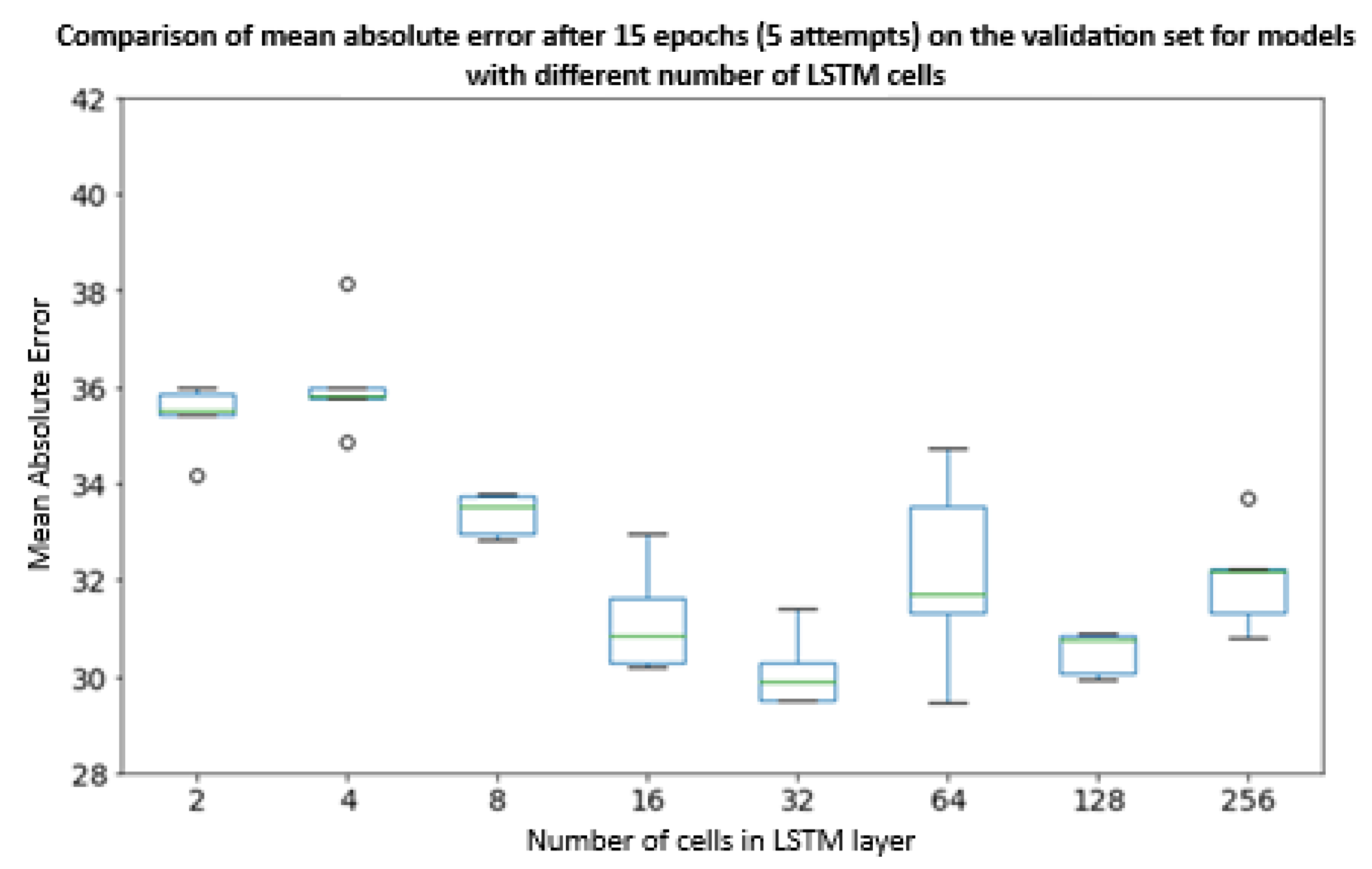
Figure 12.
Graph of the interquartile range of the mean absolute error of the obtained models after 15 epochs (5 approaches) [29] for the test set due to the different number of cells in a single LSTM layer.
Figure 12.
Graph of the interquartile range of the mean absolute error of the obtained models after 15 epochs (5 approaches) [29] for the test set due to the different number of cells in a single LSTM layer.
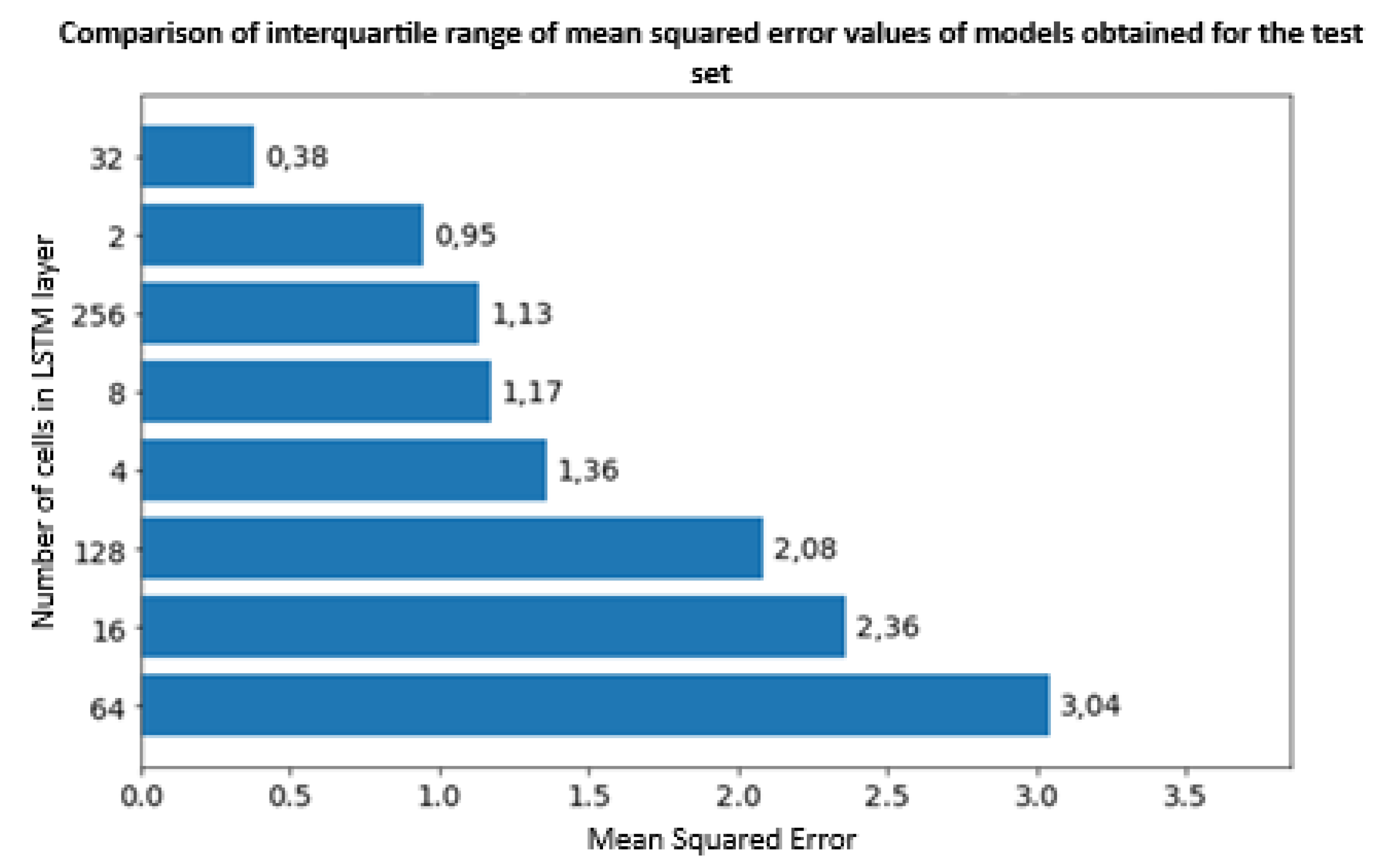
Effectively all studied cases of training, validation, testing indicate the network with the number of LSTM layer cells equal to 32 is characterized by the best stability and prediction accuracy and such a structure will be used for optimization of hyperparameters.
3.3. Hyperparameter Optimization
The hyperparameter optimization of the model containing 32 cells in the LSTM layer was performed in two stages. In the first stage, the activation function, recursive activation function, dropout, and recursive dropout were selected. The configuration of the models is shown in the table below (Table 1).
The number of training epochs increased to 100. The number of epochs to stop after no improvement in the loss function increased to 10. Each model has been trained once. The evaluation of the test model is shown in Figure 13, below.
In terms of the mean square error value for the test set, the smallest error was shown by models numbered 11, 8, 13 and 12 (Figure 13). Of these models, only model number 12 is in the top four best models evaluated for the validation set. The remaining models are characterized by larger errors.
The smallest error for the test was shown by models numbered 12, 15, 10 and 11 (Figure 14). Of these models, the top four best models evaluated for the validation set are models numbered 12 and 10. The remaining models have a larger errors. Based on the analysis, model number 11 was selected as the best model, due to the smallest mean square error and one of the smallest mean absolute errors for the test set. The model with a sigmoid activation function, hyperbolic tangent as a recursive activation function, dropout equal to 0.2 and recursive dropout equal to 0.1 will be used in the next stage of hyperparameter optimization.
In the second stage of hyperparameter optimization, the kernel and recursive regularization functions were selected. The model configuration is shown in the table below (Table 2).
The number of 100 training epochs was maintained, as well as the number of 10 epochs after which training is stopped due to the lack of improvement in the loss function value for the validation set. Each of the given models was trained once. The evaluation of the test model is shown below.
Figure 15.
Comparison of the mean square error values of the obtained models in the second stage of hyperparameter optimization for the test set.
Figure 15.
Comparison of the mean square error values of the obtained models in the second stage of hyperparameter optimization for the test set.
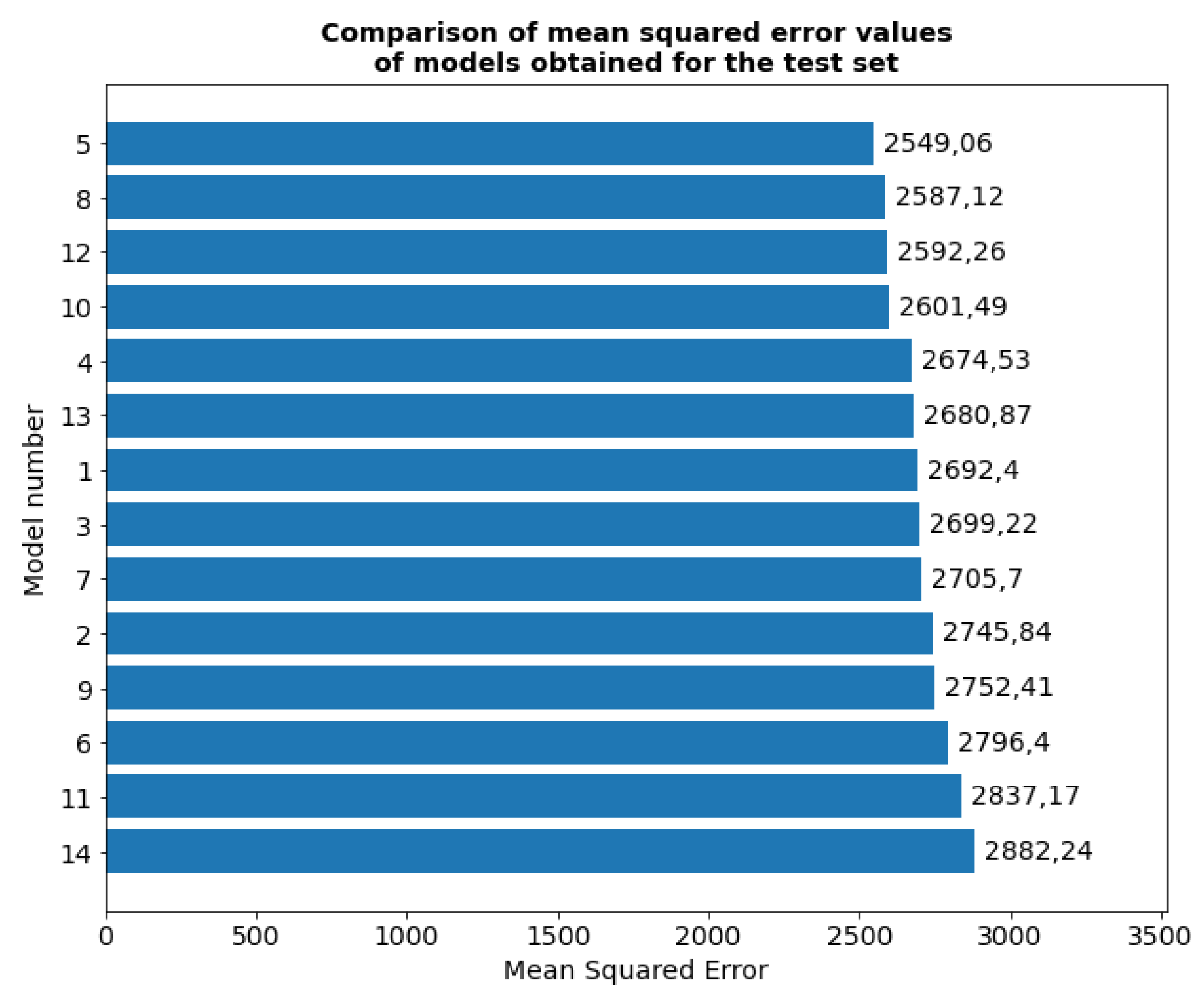
Figure 16.
Comparison of the mean absolute error values of the obtained models in the second stage of hyperparameter optimization for the test set.
Figure 16.
Comparison of the mean absolute error values of the obtained models in the second stage of hyperparameter optimization for the test set.
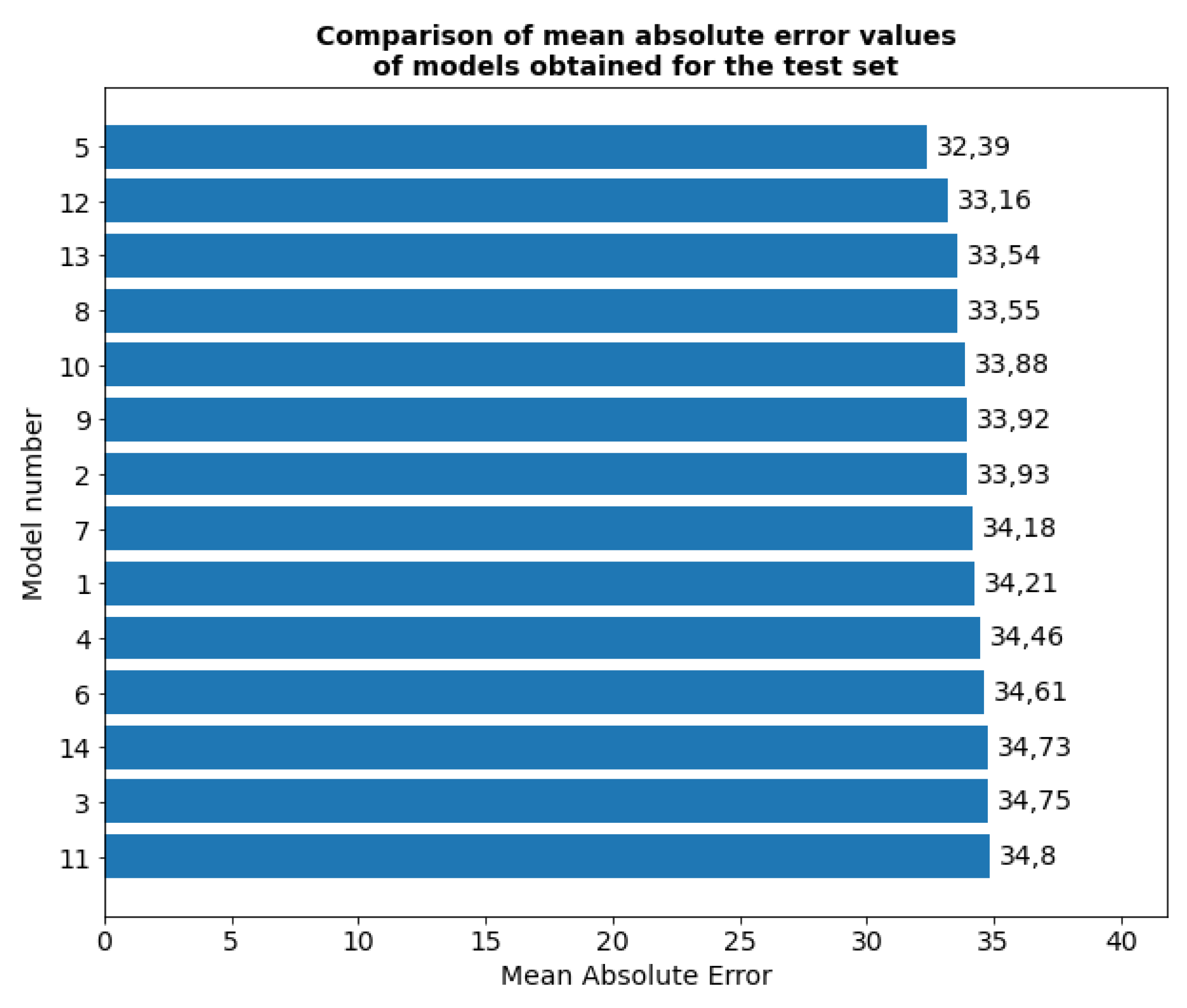
Based on the analysis of the results of the 2nd stage of optimization, the best model turned out to be model number 5, which has an L1 kernel regularization function and a recursive one.
3.4. Evaluation of the Best Neural Network Model
As a result of the optimization of the structure and hyperparameters of the recurrent LSTM neural network, a model containing 32 cells in the hidden layer, a sigmoid activation function, a hyperbolic tangent as the recursive activation function, a dropout of 0.2, a recursive dropout of 0.1, and L1 as the kernel regularization function and the recursive regularization function was selected. Below is the analysis of the learning process and the error values for individual observations from the validation and testing sets.
From the course of the learning process (Figure 17 and Figure18) it can be concluded that the model started the overfitting phase in epoch 18. From this epoch the value of the loss function for the validation set started to increase despite the decreasing value for the training set. The stop function detected this dependence and ended the learning process after 27 epochs, and the model weights were restored to the values from epoch 16 (the lowest value of the loss function for the validation set).
The histogram of the observation error (Figure 18) indicates an even distribution of errors between the training, validation and test sets. The concentration of the error value around value 0 is also visible, in the range [-34.4; 41.7) there are 73.4% of all measurements. However, the entire range of the errors is from -364.6 to 143.3 with a tendency to underestimate the measurement values. Further analysis showed that 99% of the measurements in the range from percentile 0.5 to 99.5 are in the range from -203.3 to 81.7. In turn, 95% of the measurements in the range from percentile 2.5 to 97.5 are in the range from -132.3 to 61 (Figure 19).
Then, the absolute error was analyzed using a similar method. A one-sided interval was evaluated.
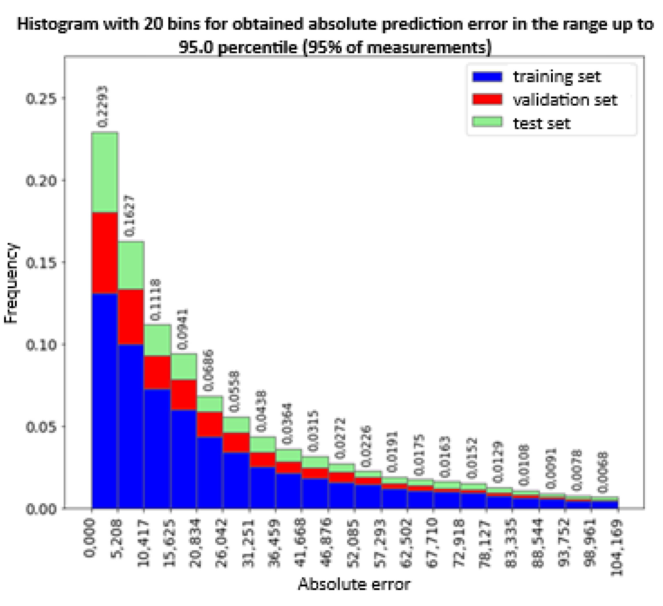
The histograms of the absolute error value (Figure 21 and Figure 22) confirm a correct distribution of errors between the training, validation and test sets. A one-sided distribution of the error value is also visible - close to the value of 0. In the range of up to 36.5 kWh of the error, 72.8% of all hourly measurements of electricity consumption are found. Further analysis showed that 99% of measurements have an error of less than 173.5 kWh of hourly electricity consumption (Figure 21). On the other hand, 95% of measurements have an error of less than 104.169 kWh of hourly electricity consumption (Figure 22). Optimization of the structure of the neural network with one LSTM layer showed that the network with 32 cells in the LSTM layer is the most optimal size of the neural network among the tested sizes from 2 to 256 cells. Which indicates that depending on the complexity of the problem being studied, both a too simple and too complex neural network will not be characterized by the best prediction accuracy. Further optimization of hyperparameters allowed for the selection of model parameters that are characterized by the lack of overfitting to the training set.
Figure 20.
Histogram of the absolute prediction error of individual observations for all sets.
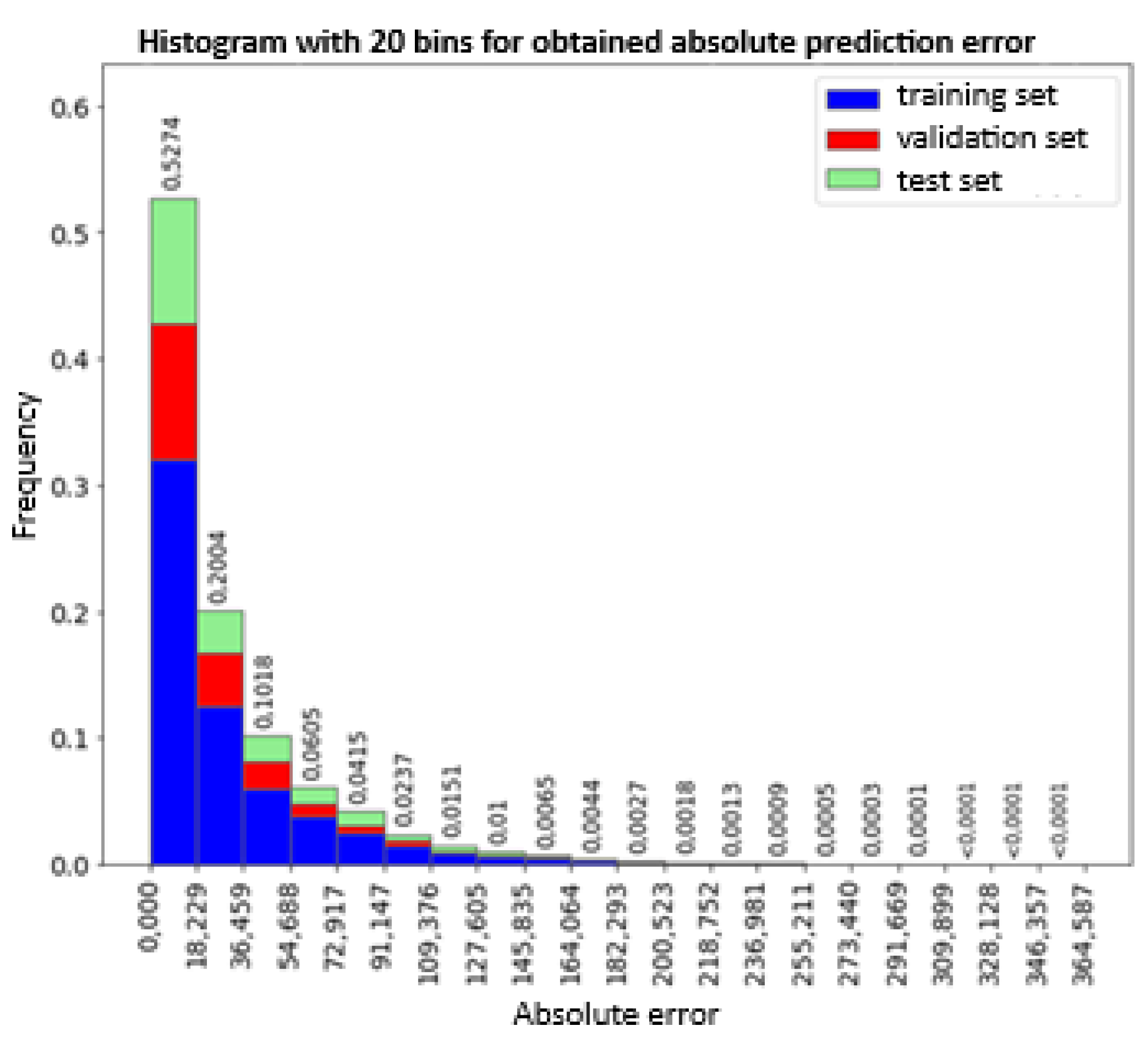
Figure 21.
Histogram of the absolute prediction error of 99% of the observations falling within the 99th percentile for all data sets.
Figure 21.
Histogram of the absolute prediction error of 99% of the observations falling within the 99th percentile for all data sets.
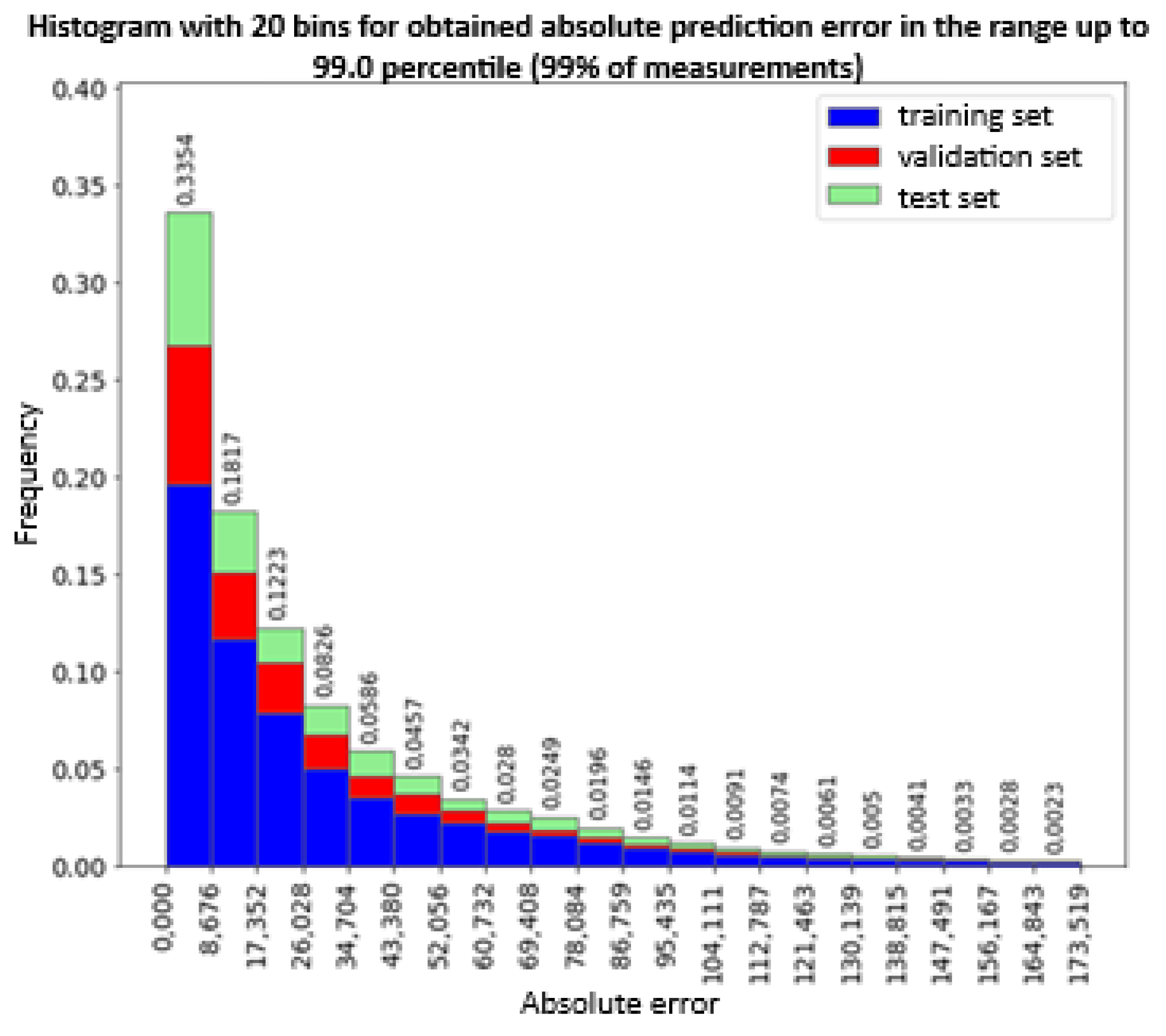
Figure 22.
Histogram of the absolute prediction error of 95% of the observations falling within the 95th percentile for all data sets.
Figure 22.
Histogram of the absolute prediction error of 95% of the observations falling within the 95th percentile for all data sets.
4. Discussion
A definition of human intelligence (Oxford Dictionary) includes: (1) cognitive ability: to learn, understand, and think logically, (2) adaptability: effectively utilize knowledge and skills in novel circumstances, (3) reasoning and problem-solving: to analyze information, and apply reason to solve problems. Being smart typically means being more practical and having adaptable intelligence, particularly in everyday life. Despite of the fact that those definitions do not involve time, both in smart and in intelligence testing, short period is involved.
In the learning stage, AI builds relationships and carry them to any new situation assuming that they are like those encountered in the learning stage. Thus, the precision of AI evaluation depends on how well the input file is prepared and whether all impact factors are included in the analyzed matrix. A more complex LSTM network, with two, three or more LSTM layers, could have higher precision, however, at the expense of the training speed. We have, decided to use one LSTM layer because our objective was not related to the model precision, but to the question of whether or not, one may construct a universal, weather dependent energy model for space heating and cooling.
Such a model had to include all variables, tall and small buildings, hot and cold climates, important and not important characteristics for measured energy, building and weather. In the input data was no air tightness of the building, because this critical building characteristics is only used in North America and Germany. Furthermore, the data were scaled (normalized), to the range (0, 1) modifying impact of all factors. For this reason, the precision shown in the absolute error characterization (Figure 21 and Figure 22) can only be considered as measure of data set consistency not does not characterize the buildings. The results shown in this paper indicated that a universal energy model for different climates and diverse building characteristics can be developed, for any defined type of building.
5. Future Research
As the conclusion of this work indicates the energy solution though a universal energy modeling, we may now define how the final energy model will look like. It will contain three sub-models, each with different precision that may be integrated or not, depending on the quality of monitoring results that can now be precisely defined. Monitoring must be included in the design of any new or retrofitting building. The future energy model will include three parts.
- Part one is identical to what we do now, except for using hourly data for transmission of heat through the whole building enclosure system (opaque and glazed together).
- Part two relates to air flow through the building enclosure. As a minimum it requires whole building airtightness characterization. We recommend that for each dwelling evaluated we require also hourly measurements of the air pressure difference in between the selected indoor and outdoor locations. Those measurements must be performed at the same height above ground. Furthermore, the information about exterior wall orientation, prevailing wind orientation, the height of the dwelling and the total building height must be included in the monitoring data.
- Part three relates to the solar gains for the evaluated dwelling, we do not specify at this stage because there is not enough practical experience but it is likely that hourly measurement of total solar radiation on horizontal planes (e.g. roof) will be required in addition to some characterization of ambient conditions.
6. Conclusions
Using the hourly data from diverse, non-residential buildings and review of literature led us to constructing a globalized, universal AI model. Preparation of data removed 64 buildings classified as outliers. Hourly measurements of electrical use, weather and building characteristics were presented for which unidirectional and recurrent neural networks. Measurement data are divided into training, validation and learning sets and prepared for a long-term system and short-term memory (LSTM) model. Optimization of the ANN gave 32 cells in one LSTM layer. This model was further optimized for hyperparameters to find the smallest mean square and mean absolute error for the test set.
The best LSTM model was a neural network with a sigmoid activation function and hyperbolic tangent as a recursive activation function. The dropout coefficient is 0.2, and the recursive dropout - 0.1. The L1 function (lasso regression) was determined to be the best function of kernel regularization and recursive regularization. A generalized model for predicting hourly electricity consumption for non-residential buildings based on weather conditions was created and the analysis results confirm that AI model may be created for heating and cooling of any universal, climate modified technology for new or retrofitted buildings.
Nevertheless, the same data analysis revealed significant differences in the variation of efficiency values for different buildings. The prediction error of the observations ranges from -134.3 kWh to 61 kWh for 95% of the measurements. The maximum absolute error for 95% of the measurements is 104.2 kWh (Figure 22), The mean absolute error was 32.4 kWh that in comparison to mean hourly electrical consumption of 77kWh (see Figure 9) is 40%, indicating a need for much more precise building categorization.
Author Contributions
Conceptualization, A.R., M.D., P.D.; methodology A.R., M.D., P.D.; software P.D., M.D., M.G., A.R.; validation P.D., M.G.; formal analysis P.D., M.D., A.R.; investigation, P.D.; resources P.D., A.R., S.K.; data curation P.D., M.G.; writing—original draft preparation, P.D., M.D; writing, P.D., M.D., A.R., MB, S.K.; review and editing A.R., M.B.; visualization, P.D., M.G.; supervision, A.R., M.D., P.D.; project administration, A.R., M.D., P.D. All authors have read and agreed to the published version of the manuscript.
Funding
This research received no external funding.
Conflicts of Interest
The authors declare no conflicts of interest.
References
- Romanska-Zapala A. and M., Bomberg, Can artificial neuron networks be used for control of HVAC in Environmental Quality Management systems? CESBE Conference, July 3, 2019, Prague, Czech Republic.
- Romanska-Zapala A., P. Dudek, M. Górny and M. Dudzik, Modular statistical system for an integrated environmental control, NSB 2020 Conference proceed, Sept 6-9, 2020 Tallinn, Estonia 621.
- Dudzik M, Anna Romanska-Zapala and Mark Bomberg,2020, A neural network for monitoring and characterization of buildings with 1 Environmental Quality Management, Part 1: Verification under steady state conditions.
- Dudzik, M. Towards Characterization of Indoor Environment in Smart Buildings: Modelling PMV Index Using Neural Network with One Hidden Layer. Sustainability 2020, 12, 6749. [Google Scholar] [CrossRef]
- Bomberg M., D.W., Yarbrough, and H. Saber, Retrofitting, energy efficency and indoor envirornment in Buildings.
- Salehinejad H., Sankar S., Barfett J., Colak E., Valaee S., (2018). Recent Advances in Recurrent Neural Networks, arXiv:1801.01078 [cs.NE], acsess22 Feb 2018. arXiv:1801.01078 [cs.
- Bushkovskyi, O. HOW BUSINESS CAN BENEFIT FROM RECURRENT NEURAL NETWORKS: 8 MAJOR APPLICATIONS, https://theappsolutions.com/blog/development/recurrent-neural-networks/ (access 03.09.2022).
- Brownlee, J. How to Use Standard Scaler and MinMaxScaler Transforms in Python, https://machinelearningmastery.com/standardscaler-and-minmaxscaler-transforms-in-python/ 2020 , (access 03.09.2022).
- Olah, Ch. 2015, Understanding LSTM Networks, https://colah.github.io/posts/2015-08-Understanding-LSTMs/, (access 04.09.2022).
- Calzone, O. 2021, An Intuitive Explanation of LSTM, https://medium.com/@ottaviocalzone/an-intuitive-explanation-of-lstm-a035eb6ab42c, 2021, (access 04.09.2022).
- Clayton M., Forrest M.. The Building Data Genome Project: An open, public data set from non-residential building electrical meters, Energy Procedia, Volume 122, September 2017, Pages 439-444, ISSN 1876-6102.
- Clayton M., Tian J. Building Data Genome Project 1, https://www.kaggle.com/datasets/claytonmiller/building-data-genome-project-v1, 2017 (access 26.08.2022).
- Clayton, M. , Screening Meter Data: Characterization of Temporal Energy Data from Large Groups of Non-Residential Buildings, ETH Zürich, 2017.
- Clayton M., Forrest M. Mining electrical meter data to predict principal building use, performance class, and operations strategy for hundreds of non-residential building, Energy and Buildings, 156, 2017 (Supplement C), 360–373.
- Clayton, M. What's in the box?! Towards explainable machine learning applied to non-residential building smart meter classification, Energy and Buildings 199, 2019, 523-536.
- Koste, K. Exploration, Clustering, and Day-Ahead Forecasting, https://www.kaggle.com/code/kevinkoste/exploration-clustering-and-day-ahead-forecasting, 2019, (access 26.08.2022).
- Fu, C. Timeseries FDD using an Autoencoder [meters], https://www.kaggle.com/code/patrick0302/timeseries-fdd-using-an-autoencoder-meters, 2020 (access 26.08.2022).
- Fu, C. , Prediction results in New York, https://www.kaggle.com/code/patrick0302/prediction-results-in-new-york, 2020 (access 26.08.2022).
- Bohao, X. Classify the target offices in client-group1, https://www.kaggle.com/code/xibohao/classify-the-target-offices-in-client-group1, 2020 (access 26.08.2022).
- Zhenyu, D. Models accuracy comparison for Phoenix, https://www.kaggle.com/code/douzhenyu/models-accuracy-comparison-for-phoenix, 2021 (access 26.08.2022).
- How the 1-100 ENERGY STAR Score is Calculated, https://www.energystar.gov/buildings/benchmark/understand_metrics/how_score_calculated (access 29.08.2022).
- Find out what a Building Energy Rating (BER) Certificate means for a property's energy efficiency and how it is calculated., https://www.seai.ie/home-energy/building-energy-rating-ber/understand-a-ber-rating/ (access 29.08.2022).
- What Is the Interquartile Range Rule? How to Detect the Presence of Outliers, https://www.thoughtco.com/what-is-the-interquartile-range-rule-3126244 (access 29.08.2022).
- Hancock, J.T.; Khoshgoftaar, T.M. Survey on categorical data for neural networks. J Big Data 2020, 7, 28. [Google Scholar] [CrossRef]
- Sazlı M. H, . A brief review of feed-forward neural networks, Communications Faculty of Sciences University of Ankara Series A2-A3 Physical Sciences and Engineering, vol. 50, no. 01, pp. 0-0, Jan. 2006.
- Feng W., 19. Neural Network, https://runawayhorse001.github.io/LearningApacheSpark/fnn.html, 2017 (access 03.09.2022).
- Melcher, K. A Friendly Introduction to [Deep] Neural Networks, https://www.knime.com/blog/a-friendly-introduction-to-deep-neural-networks, 2021 (access 03.09.2022).
- Brownlee, J. Gentle Introduction to the Adam Optimization Algorithm for Deep Learning, https://machinelearningmastery.com/adam-optimization-algorithm-for-deep-learning/ , 2017, (access 03.09.2022).
- Prakharry. Intuition of Adam Optimizer, https://www.geeksforgeeks.org/intuition-of-adam-optimizer/ 2020 , (access 03.09.2022).
- Overfitting. Learn how to avoid overfitting, so that you can generalize data outside of your model accurately, https://www.ibm.com/cloud/learn/overfitting, 2021 (access 03.09.2022).
- Pykes, A. Fighting Overfitting With L1 or L2 Regularization: Which One Is Better?, https://neptune.ai/blog/fighting-overfitting-with-l1-or-l2-regularization, 2022 (access 03.09.2022).
- Brownlee, J. A Gentle Introduction to Dropout for Regularizing Deep Neural Networks, https://machinelearningmastery.com/dropout-for-regularizing-deep-neural-networks/ , 2018, (access 03.09.2022).
Figure 1.
Energy efficiency histogram (frequency vs value of the index).
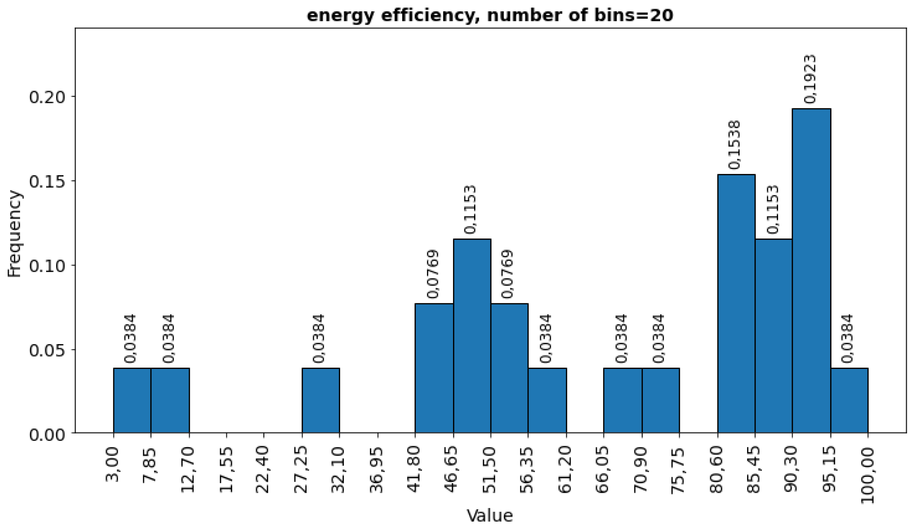
Figure 2.
Frequency of occurrence of the building's usable area.
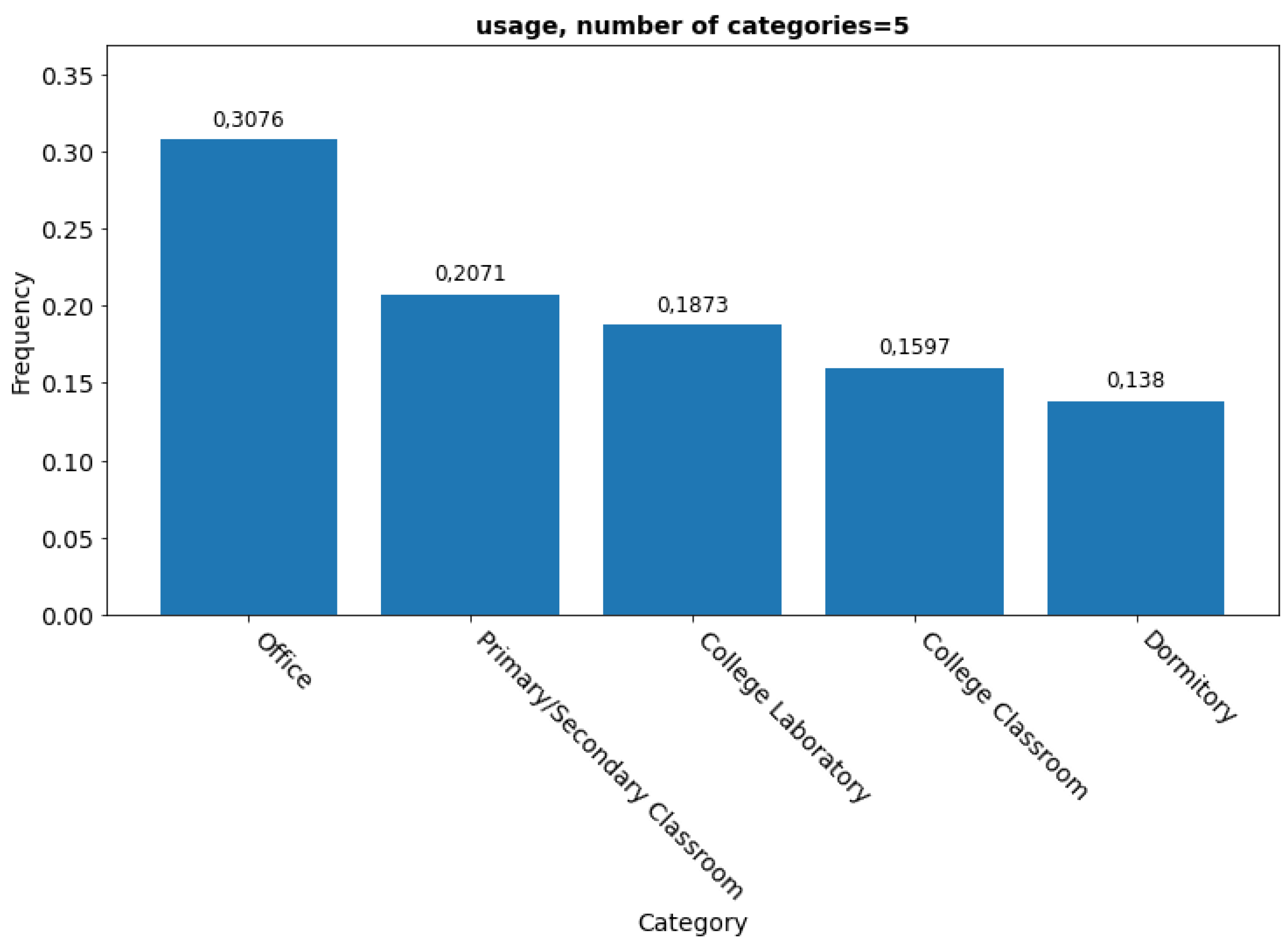
Figure 3.
Frequency of occurrence of individual energy efficiency rating (6 classes).
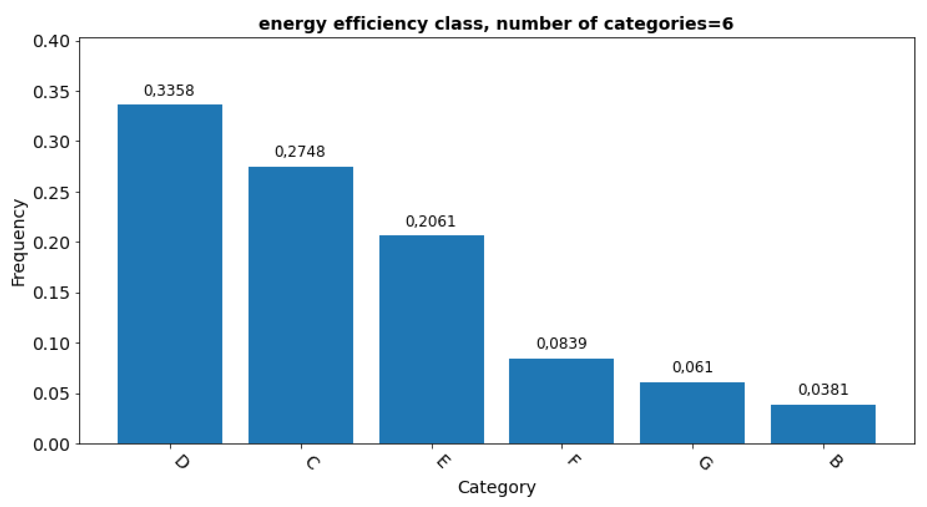
Figure 4.
Histogram of the number of floors.
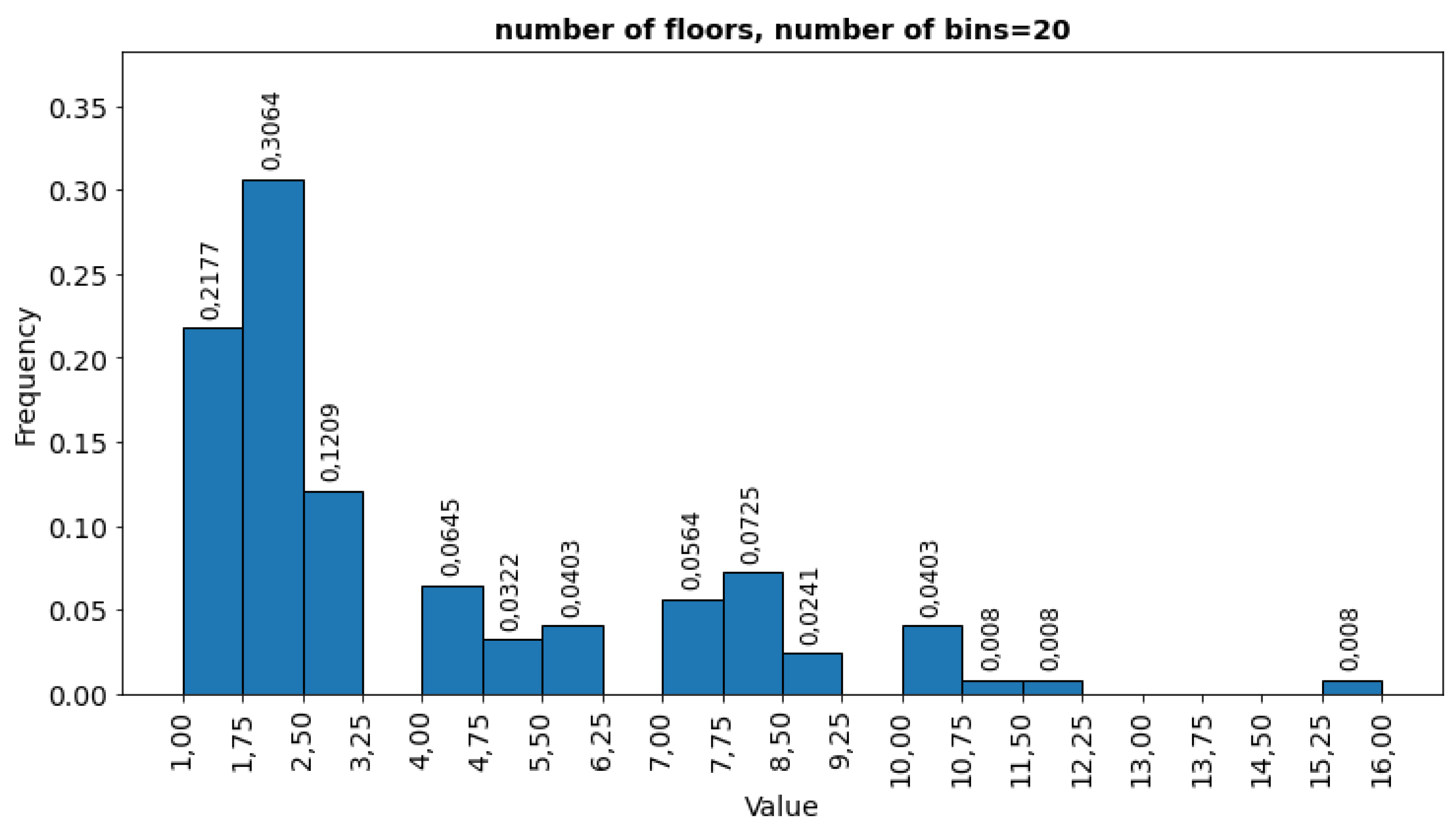
Figure 5.
Time zone frequency.
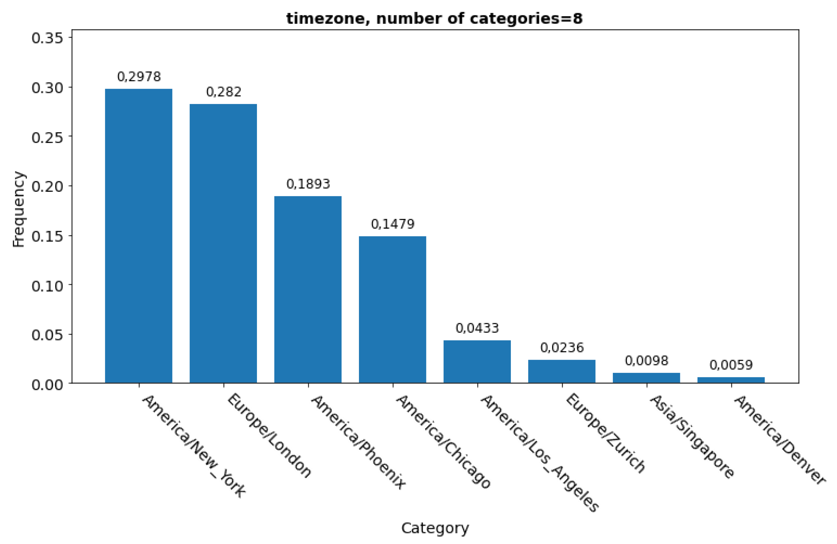
Figure 6.
Histogram of year of construction.
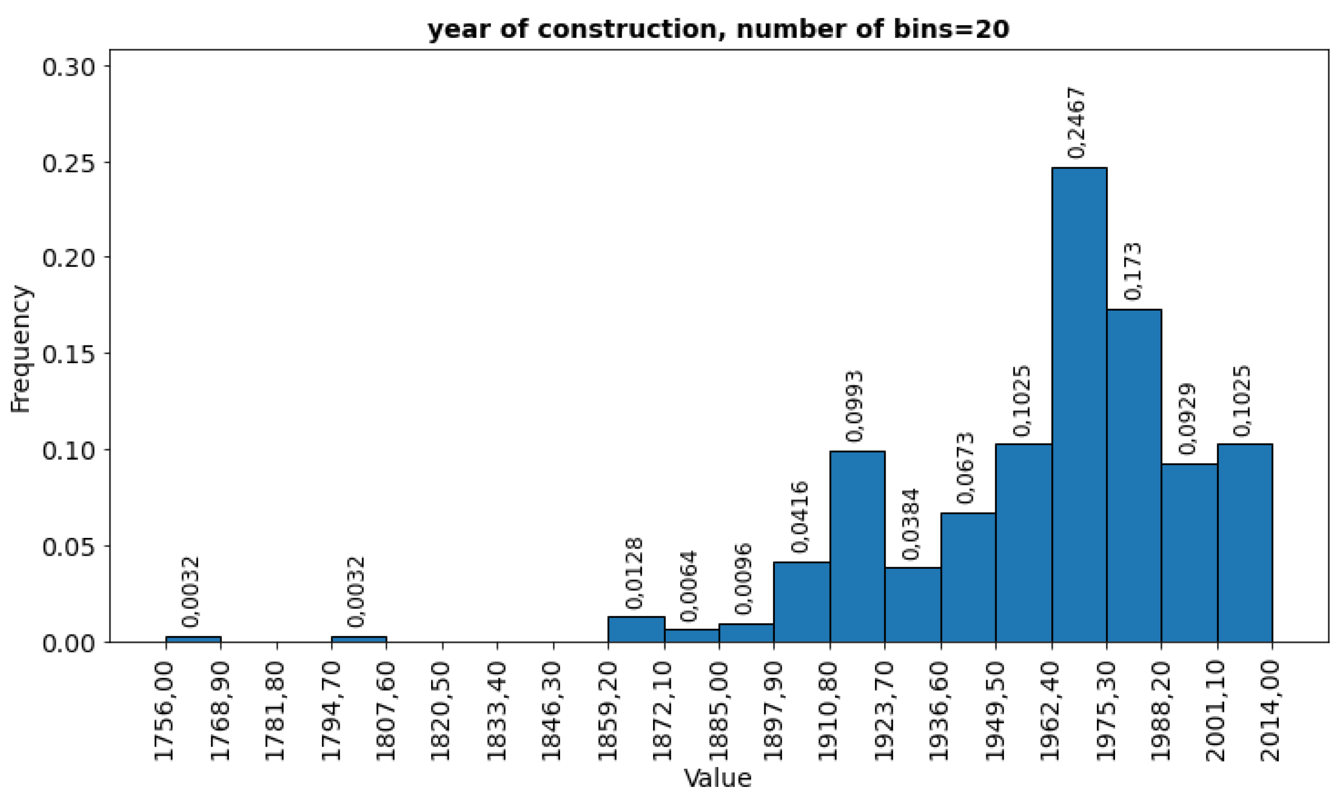
Figure 7.
Electricity consumption during the first 2 weeks of collecting electricity consumption measurements.
Figure 7.
Electricity consumption during the first 2 weeks of collecting electricity consumption measurements.
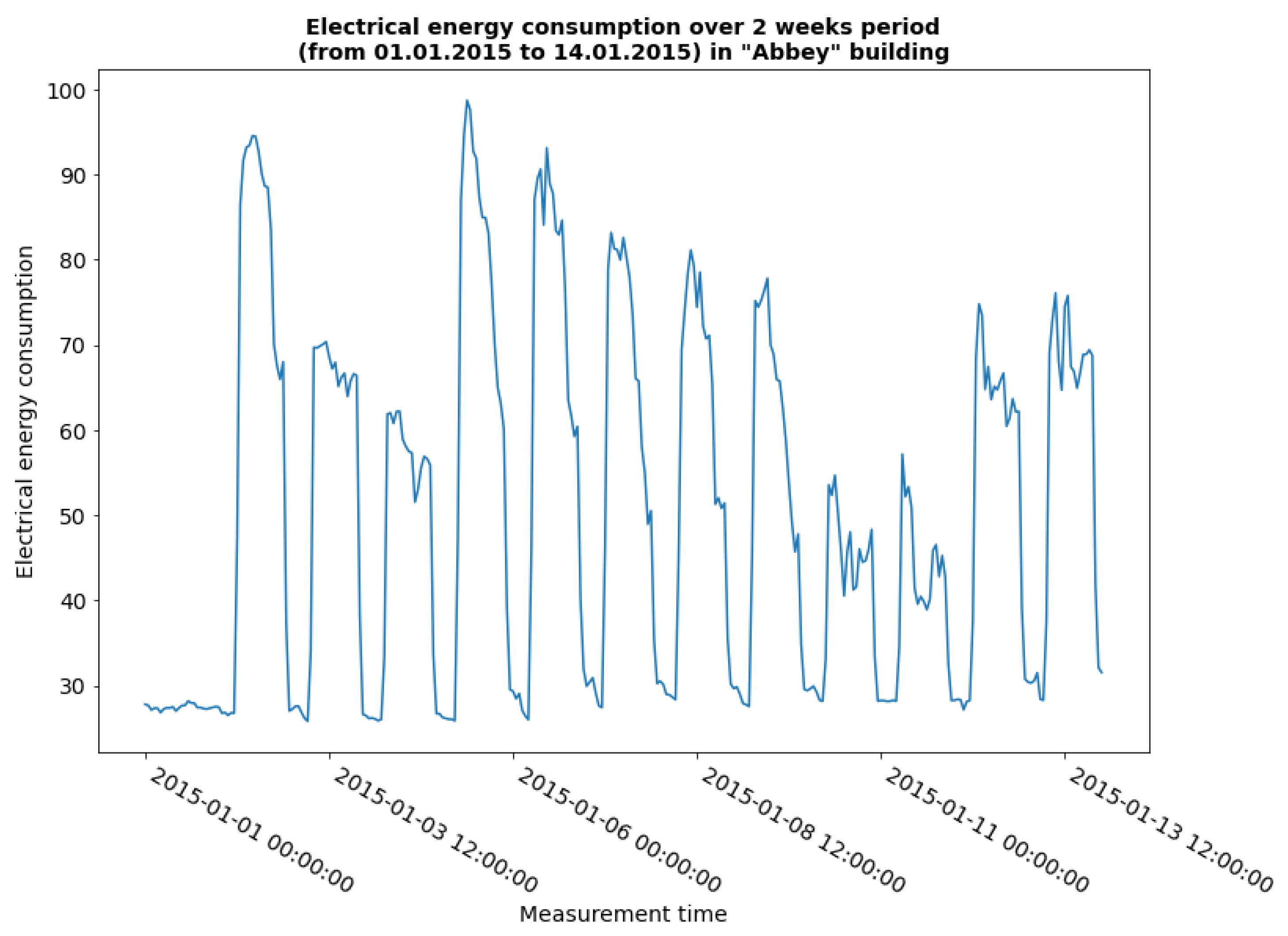
Figure 8.
Comparison of the range of electricity consumption values for the first 35 buildings from the dataset.
Figure 8.
Comparison of the range of electricity consumption values for the first 35 buildings from the dataset.
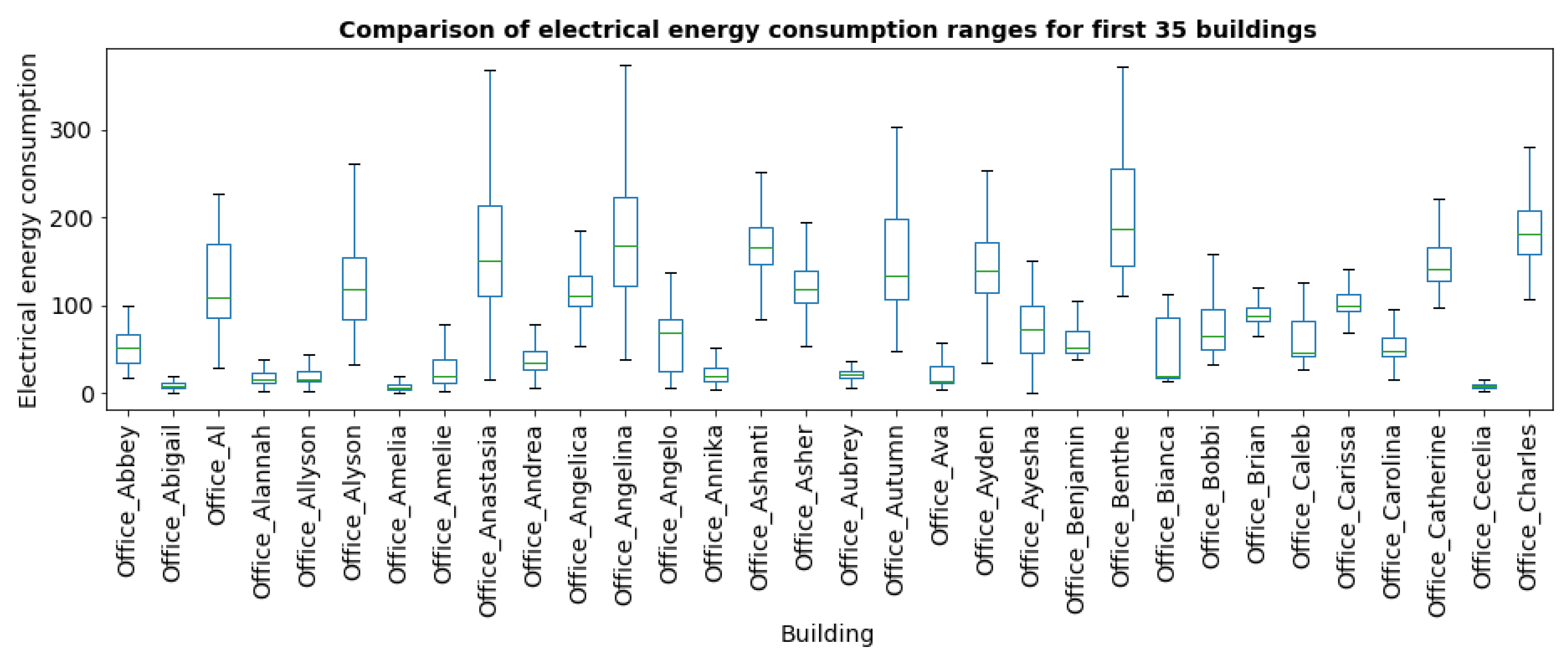
Figure 9.
Histogram of electricity consumption for buildings without outliers.
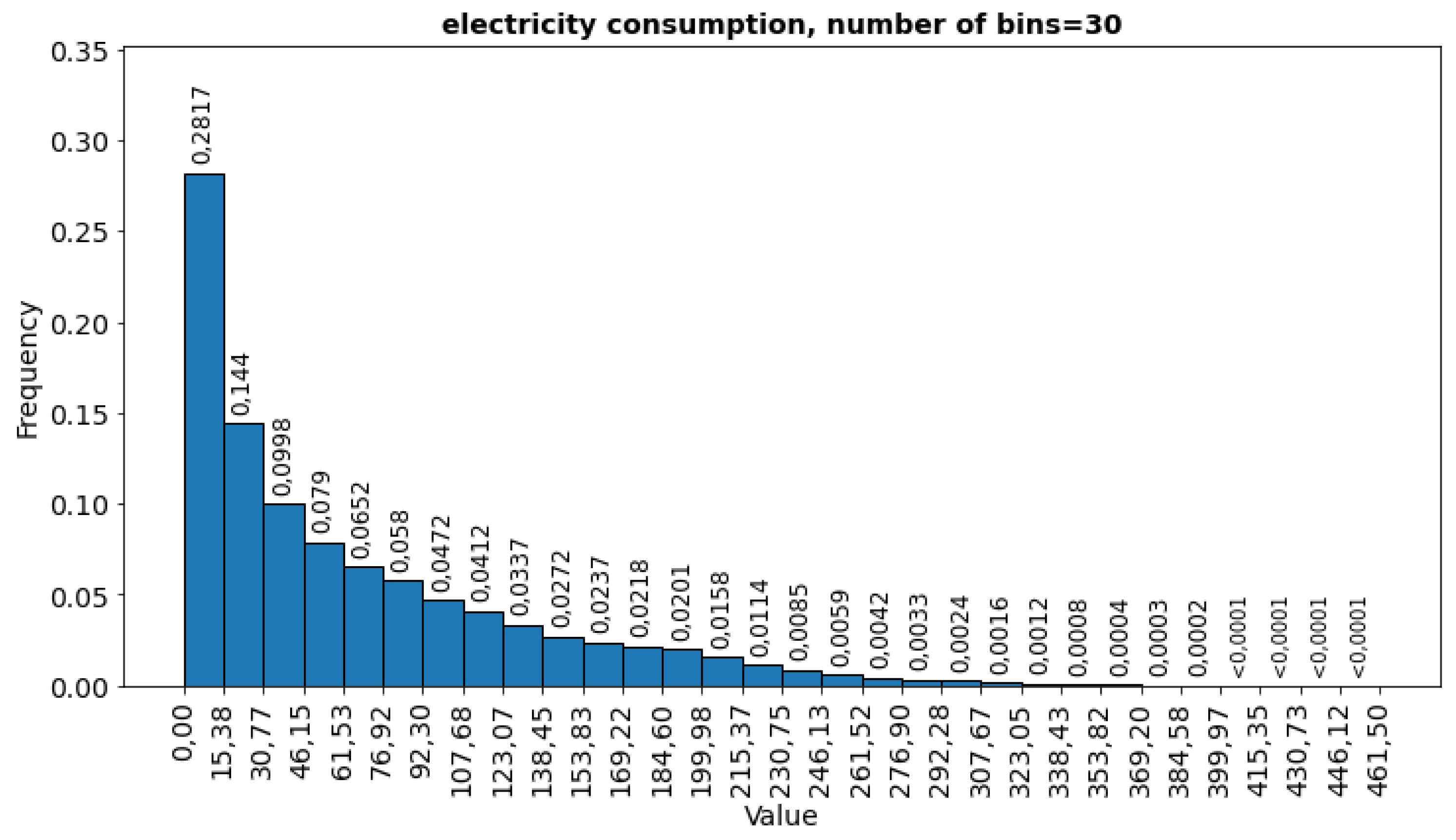
Figure 10.
Histogram for temperature [°C].
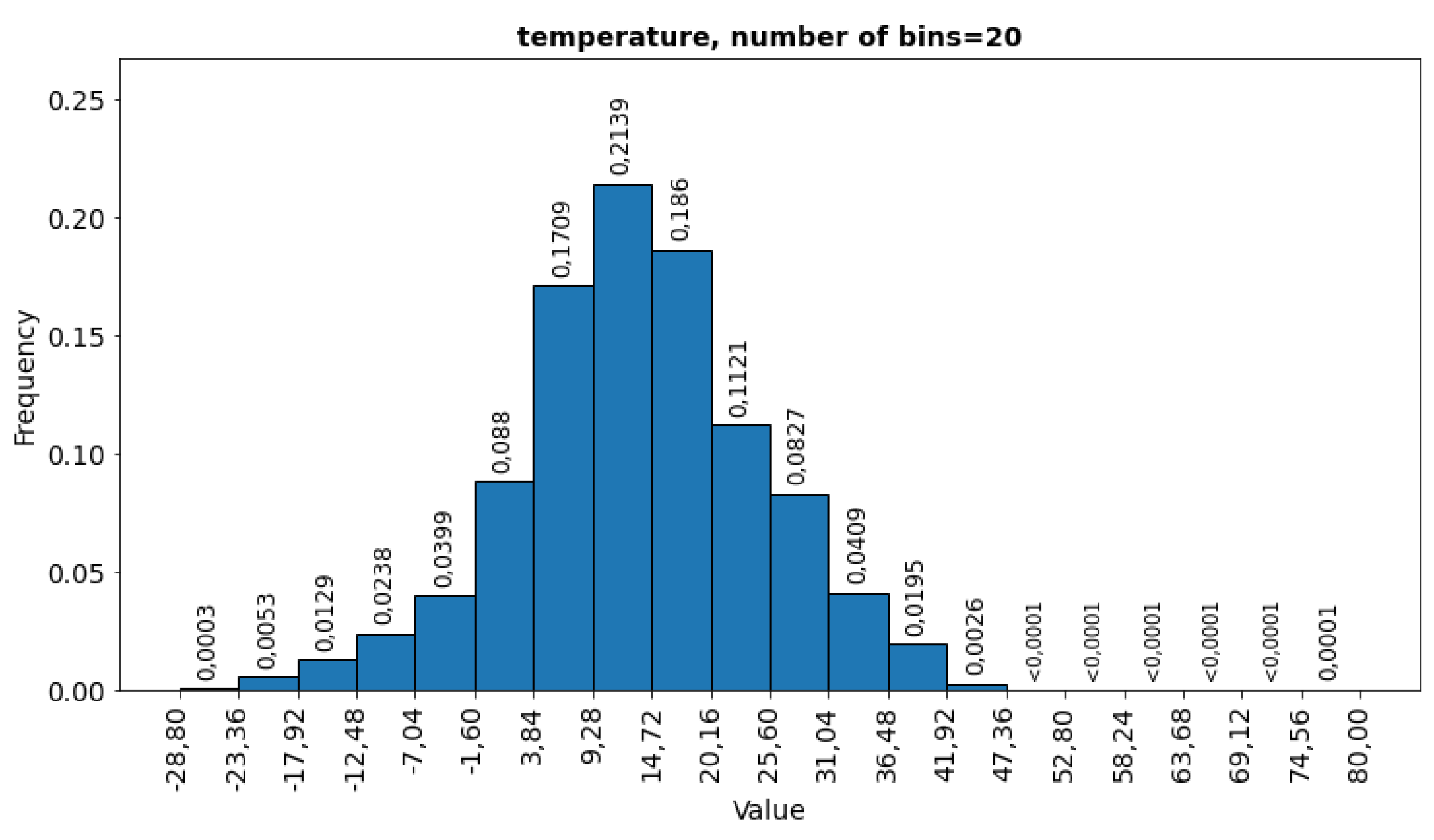
Figure 13.
Comparison of the mean square error values of the obtained models in the first stage of hyperparameter optimization for the validation set.
Figure 13.
Comparison of the mean square error values of the obtained models in the first stage of hyperparameter optimization for the validation set.
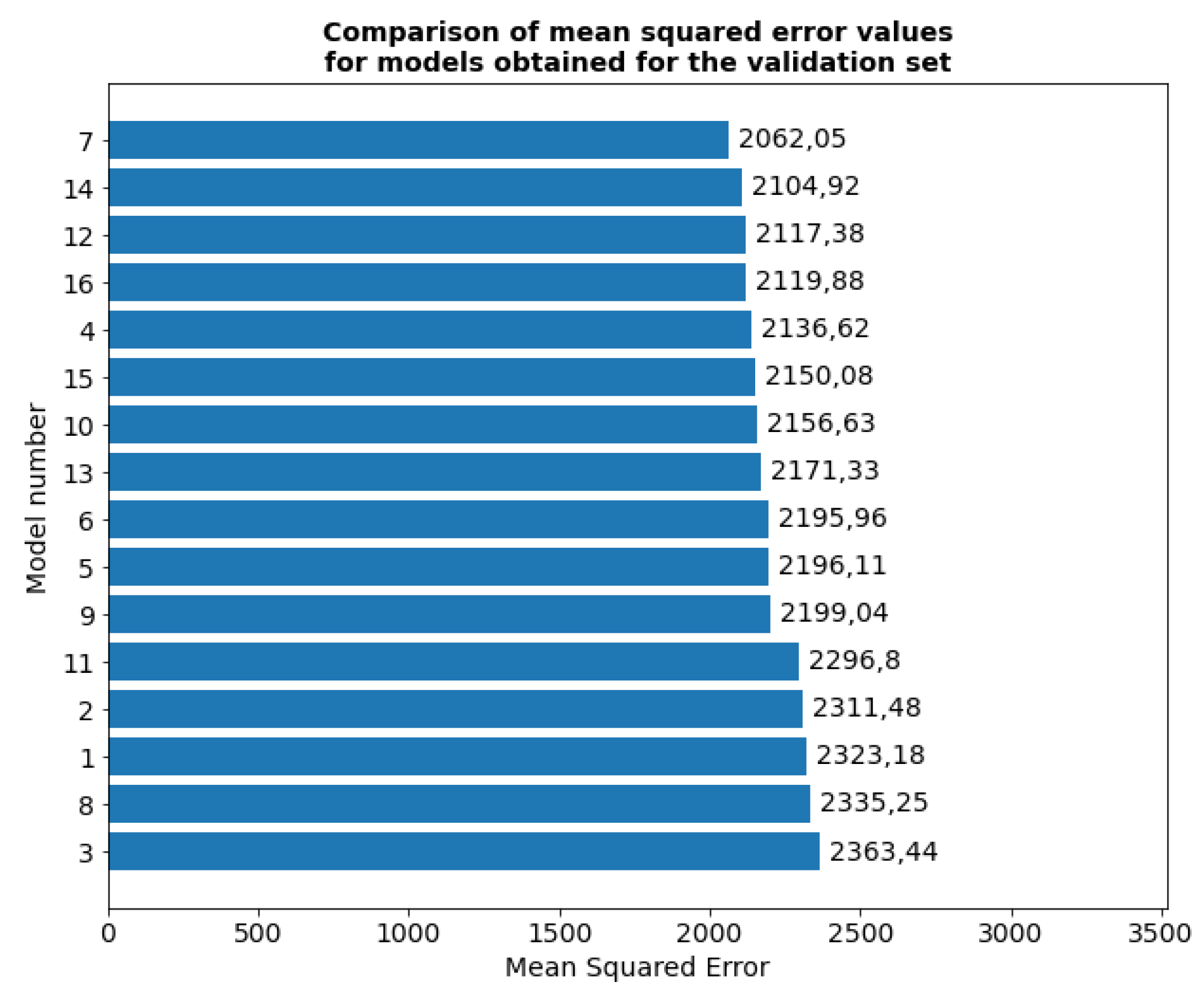
Figure 14.
Comparison of the mean absolute error values of the obtained models in the first stage of hyperparameter optimization for the test set.
Figure 14.
Comparison of the mean absolute error values of the obtained models in the first stage of hyperparameter optimization for the test set.
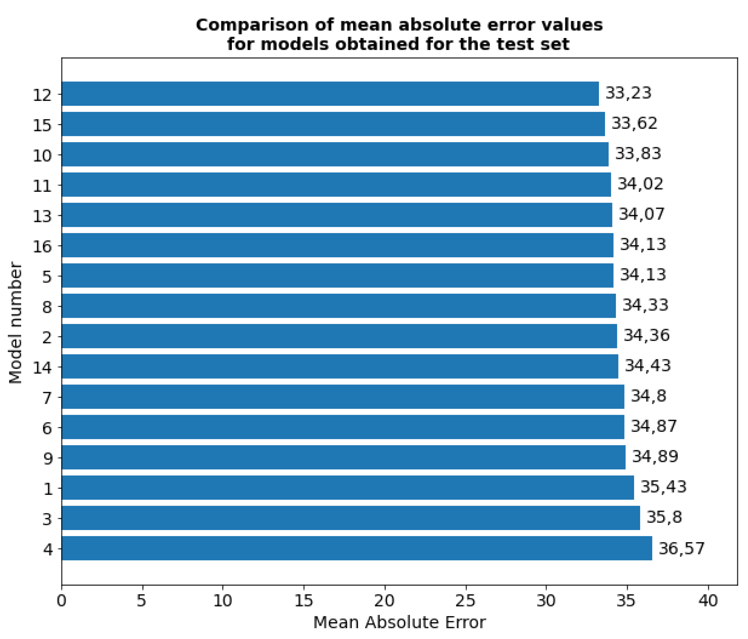
Figure 17.
The value of the mean absolute error for the training and validation sets in each epoch of model training.
Figure 17.
The value of the mean absolute error for the training and validation sets in each epoch of model training.
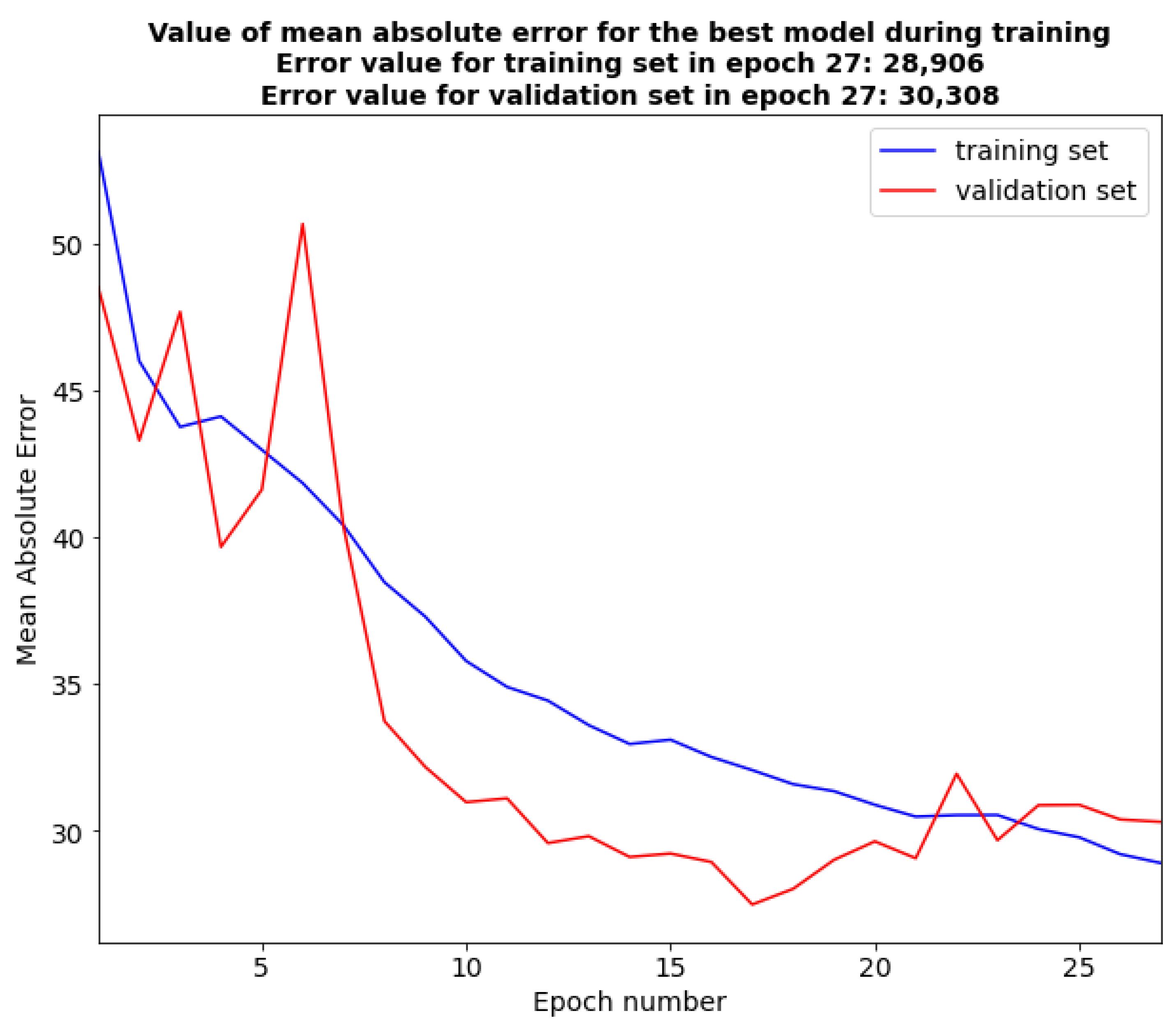
Figure 18.
Histogram of the prediction error of individual observations for all sets.
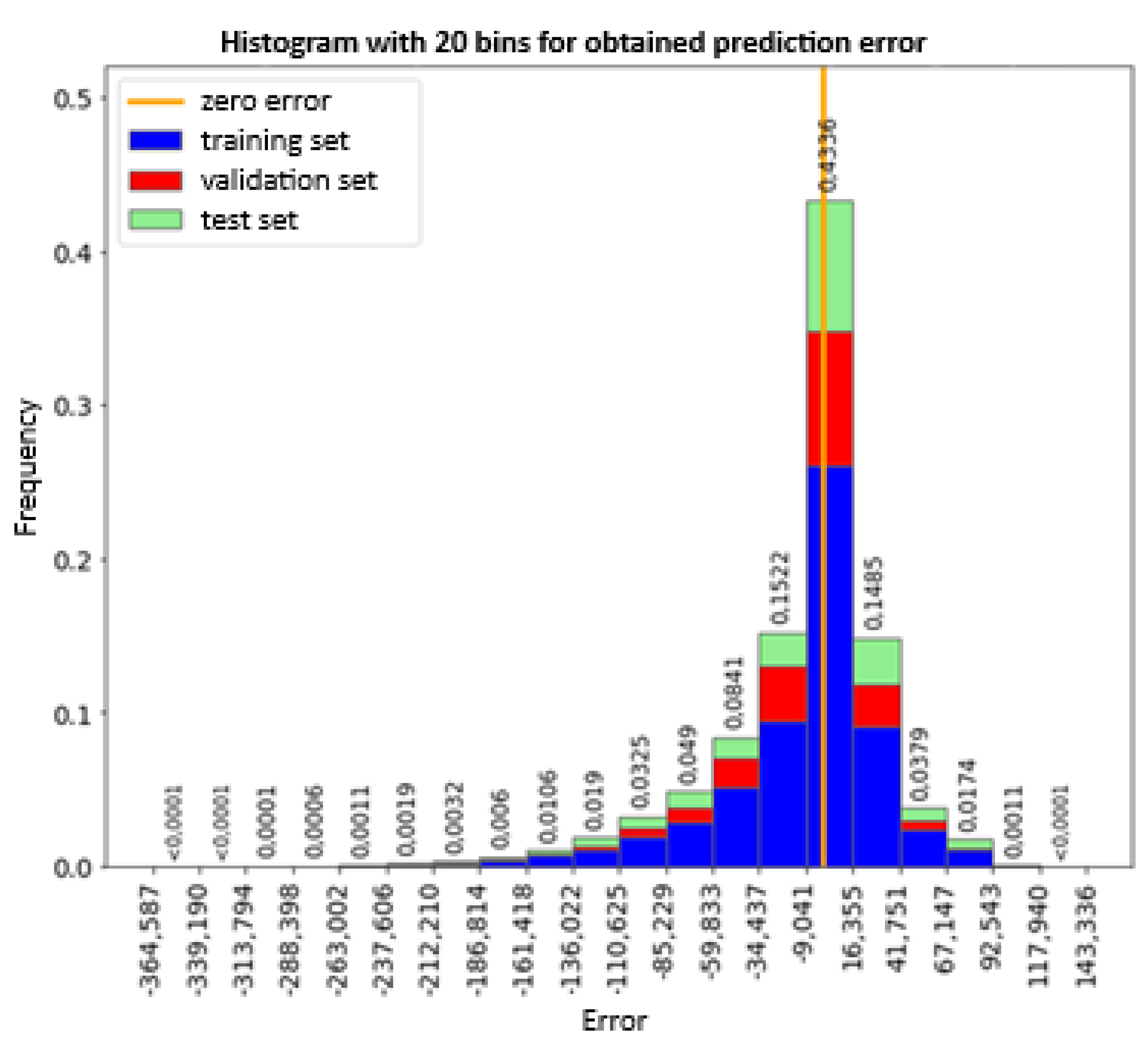
Figure 19.
Histogram of the prediction error of 95% of observations between the 2.5th and 97.5th percentile for all data sets.
Figure 19.
Histogram of the prediction error of 95% of observations between the 2.5th and 97.5th percentile for all data sets.
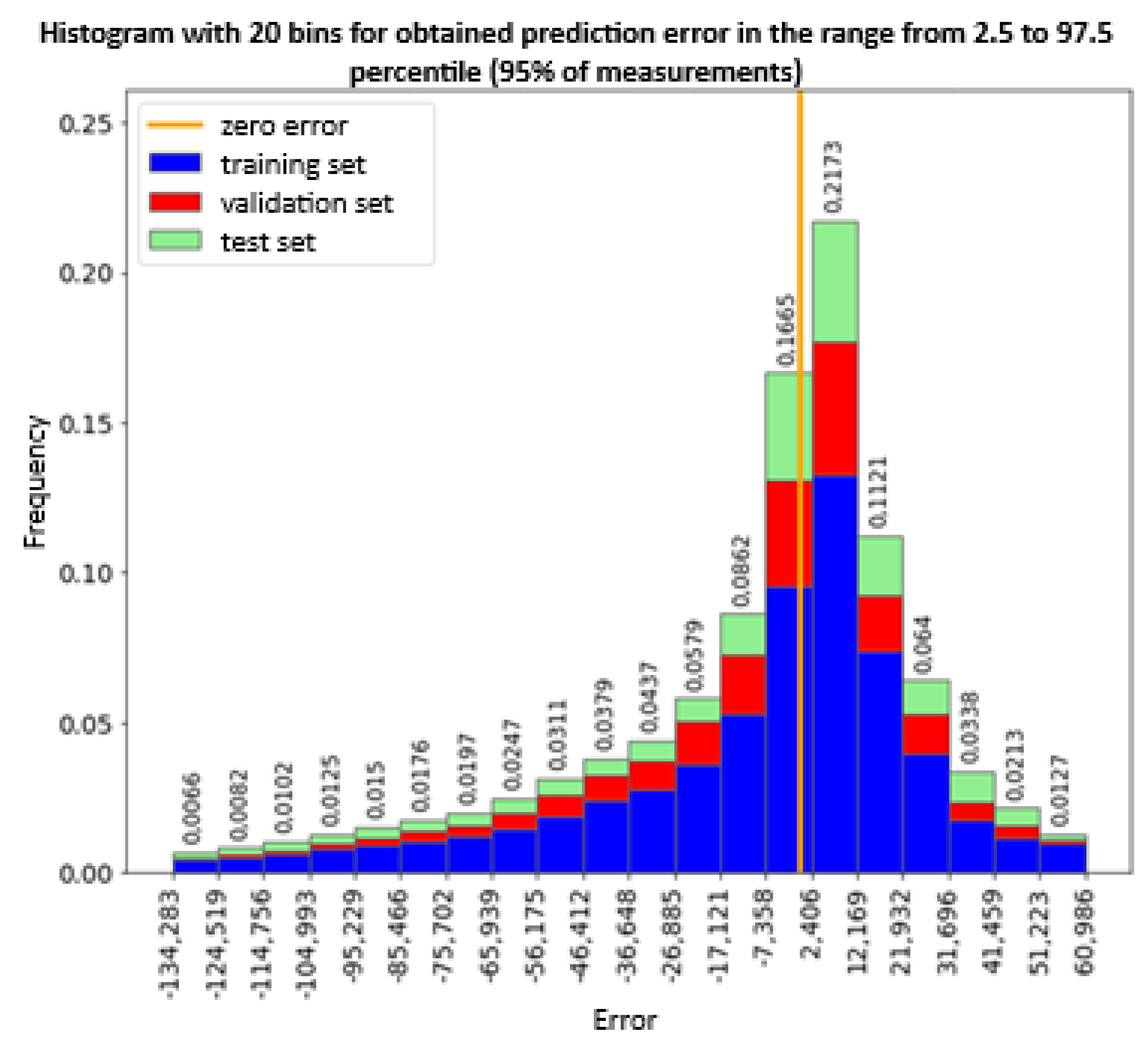

Table 1.
Configuration of activation function, recursive activation function, dropout and recursive dropout hyperparameter optimization models.
Table 1.
Configuration of activation function, recursive activation function, dropout and recursive dropout hyperparameter optimization models.
| Model Number | Activation Function | Recursive activation function | Dropout | Recursive dropout |
|---|---|---|---|---|
| 1 | hyperbolic tangent | hyperbolic tangent | 0,1 | 0,1 |
| 2 | hyperbolic tangent | hyperbolic tangent | 0,1 | 0,2 |
| 3 | hyperbolic tangent | hyperbolic tangent | 0,2 | 0,1 |
| 4 | hyperbolic tangent | hyperbolic tangent | 0,2 | 0,2 |
| 5 | hyperbolic tangent | sigmoidal | 0,1 | 0,1 |
| 6 | hyperbolic tangent | sigmoidal | 0,1 | 0,2 |
| 7 | hyperbolic tangent | sigmoidal | 0,2 | 0,1 |
| 8 | hyperbolic tangent | sigmoidal | 0,2 | 0,2 |
| 9 | sigmoidal | hyperbolic tangent | 0,1 | 0,1 |
| 10 | sigmoidal | hyperbolic tangent | 0,1 | 0,2 |
| 11 | sigmoidal | hyperbolic tangent | 0,2 | 0,1 |
| 12 | sigmoidal | hyperbolic tangent | 0,2 | 0,2 |
| 13 | sigmoidal | sigmoidal | 0,1 | 0,1 |
| 14 | sigmoidal | sigmoidal | 0,1 | 0,2 |
| 15 | sigmoidal | sigmoidal | 0,2 | 0,1 |
| 16 | sigmoidal | sigmoidal | 0,2 | 0,2 |
Table 2.
Configuration of hyperparameter optimization models of kernel and recursive regularization functions.
Table 2.
Configuration of hyperparameter optimization models of kernel and recursive regularization functions.
| Model number | Kernel regularization function | Recursive regularization function |
|---|---|---|
| 1 | - | L1 |
| 2 | - | L2 |
| 3 | - | l1l2 |
| 4 | L1 | - |
| 5 | L1 | L1 |
| 6 | L1 | L2 |
| 7 | L1 | L1L2 |
| 8 | L2 | - |
| 9 | L2 | L1 |
| 10 | L2 | L2 |
| 11 | L2 | L1L2 |
| 12 | L1L2 | - |
| 13 | L1L2 | L1 |
| 14 | L1L2 | L2 |
| 15 | L1L2 | L1L2 |
Disclaimer/Publisher’s Note: The statements, opinions and data contained in all publications are solely those of the individual author(s) and contributor(s) and not of MDPI and/or the editor(s). MDPI and/or the editor(s) disclaim responsibility for any injury to people or property resulting from any ideas, methods, instructions or products referred to in the content. |
© 2025 by the authors. Licensee MDPI, Basel, Switzerland. This article is an open access article distributed under the terms and conditions of the Creative Commons Attribution (CC BY) license (http://creativecommons.org/licenses/by/4.0/).
Copyright: This open access article is published under a Creative Commons CC BY 4.0 license, which permit the free download, distribution, and reuse, provided that the author and preprint are cited in any reuse.


