
Submitted:
15 March 2025
Posted:
17 March 2025
You are already at the latest version
Abstract
Heating, ventilation, and air conditioning (HVAC) systems account for 60% of the energy consumption in commercial buildings. Each year, millions of dollars are spent on electricity bills by commercial building operators. To address this energy consumption challenge, a predictive model named Bayesian optimisation Convolution Neural Network Multivariate Long Short-term Memory (BO CNN-M-LSTM) is introduced in this research. The proposed model is designed to perform load forecasting, optimizing energy usage in commercial buildings. The CNN block extracts local features, whereas the M-LSTM captures temporal dependencies. The hyperparameter fine tuning framework applied Bayesian optimization to enhance output prediction by modifying model properties with data characteristics. Moreover, to improve occupant well-being in commercial buildings, the thermal comfort adaptive model developed by de Dear and Brager was applied to ambient temperature in the preprocessing stage. As a result, across all four datasets, the BO CNN-M-LSTM consistently outperformed other models, achieving an 8% improvement in mean percentage absolute error (MAPE), 2% in normalized root mean square error (NRMSE), and 2% in R2 score.This indicates the consistent in performance of BO CNN-M-LSTM under varying environmental factors, highlight the model robustness and adaptability.Hence, the BO CNN-M-LSTM model is a highly effective predictive load forecasting tool for commercial building HVAC systems.
Keywords:
Load Forecasting
; Thermal Comfort
; Commercial Building
; Renewable Energy
; Control Engineering
; Deep Learning
1. Introduction
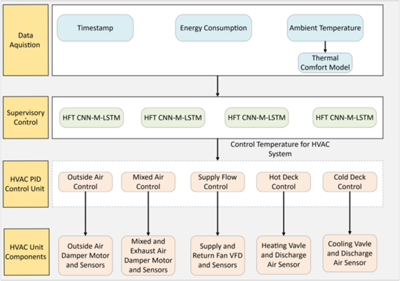
With the significant increase of energy consumption and the integration of loads into commercial buildings, energy saving scheme have become a critical direction for sustainable development. For instance, in 2022, commercial buildings made up 30% of global final energy consumption, of which 35% was in the form of electricity [1]. In a related finding, the U.S. Energy Information Administration’s 2018 Commercial Buildings Energy Consumption Survey (CBECS) [2] revealed that electricity constituted 60% of the U.S.’s energy use for commercial buildings, making it a primary energy source. Heating, ventilation, and air conditioning (HVAC) systems were the main users of this electricity, resulting in an annual expenditure of USD 119 billion, or 84% of total energy costs in commercial buildings. These figures highlight the considerable energy consumption and associated costs of HVAC systems, underscoring the pressing need for increased energy efficiency in the building sector. Therefore, the development and implementation of effective control strategies for HVAC systems is essential, as displayed in Figure 1.
The systematic review indicates that local HVAC controllers, such as process control or sequencing control, can be energy-efficient and cost-effective for specific subsystems. However, these controllers may face challenges in balancing energy efficiency, cost-effectiveness, and maintaining indoor thermal comfort. In contrast, supervisory control methods, such as machine learning and deep learning techniques, exhibit the capability to account for all characteristics, interactions among components, and their associated variables.
In particular, the demand response (DR) strategies that incentivize shifts in energy consumption patterns [4] have demonstrated significant potential for improving energy management. Given the substantial energy use of HVAC systems, optimizing their electricity consumption is particularly valuable. For instance, adaptive HVAC control systems, powered by Model Predictive Control (MPC) method [5], can dynamically adjust operations in response to real-time conditions, thus reduce electricity consumption during peak demand periods. This capability not only enhances the efficiency of DR programs but also supports power grid stability [6]. In commercial buildings, many studies [7]– 10] had applied MPC method to control zone temperatures and building thermal mass.
In a 2024 study, Wang et al. [11] highlights the pivotal role of MPC, emphasising that its hinges on the accurate forecasting of key variables, such as energy consumption, temperature, and occupancy patterns. This accuracy is critical because MPC relies on predictive models to make real-time adjustments that minimize energy use while maintaining indoor thermal comfort. Therefore, deterministic models are particularly well-suited for MPC due to their ability to deliver consistent and reproducible results, which are essential for ensuring reliable control decisions in dynamic environments. Their simplicity allows for easier implementation and faster computation, enabling real-time responsiveness, which is crucial for energy management systems. Moreover, by controllable variables and eliminating the complexity of stochastic variations, deterministic models enhance both the scalability and the practical implementation of MPC in energy management and building optimization systems. Hence, in the systematic review, our paper presents a Table 1 which displays an overview of various deterministic models utilized for electricity consumption forecasting of HVAC systems in commercial buildings.
A study by Mohan and Subathra [12] revealed that most prior research (80%) had concentrated on short-term load forecasting, with 15% addressing price forecasting for medium-term horizons, and only 5% focusing on long-term forecasting [13]. Meanwhile, hybrid deep learning models are considered optimal for long-term forecasting [14]. To rigorously evaluate its performance, we conducted a comprehensive comparative analysis against a diverse set of models, including:
Furthermore, electricity consumption in commercial buildings is influenced by several factors, such as weather conditions [17], occupancy rates [18], and building characteristics [19]. Among these, ambient temperature stands out as a key parameter driving HVAC energy usage [20]. For example, the annual power use of HVAC systems can increase by up to 12.7% in hot climates due to rising temperatures, while cold climates may see a reduction of 7.4% [21]. Therefore, to capture the indoor thermal comfort, traditional Predicted Mean Vote (PMV) model and machine learning thermal models are the best solution. A study by Qiantao Zhao [22] highlights that compared to PMV model, machine learning thermal models can create personalised comfort model and suitable for large scale deployments in smart buildings.
2. Research Gap
The systematic review highlights a reliance on uniform model architectures for both long and short-term load forecasting, limiting adaptability to data characteristics. Additionally, existing studies inadequately integrate thermal comfort in HVAC systems, often relying on the PMV model, which demands extensive data and overlooks individual variability. Addressing these gaps, this paper proposes the BO CNN-LSTM model for predictive load forecasting in commercial HVAC systems. The model enhances forecasting accuracy and adaptability while incorporating thermal comfort considerations. This research advances HVAC optimization by improving precision, efficiency, and occupant-centric performance, contributing to the development of smarter, more adaptive building management systems.
- The proposed model optimizes indoor temperatures to enhance occupant well-being while reducing energy use and protecting building loads during peak hours. It uses an adaptive thermal comfort framework that adjusts the indoor environment in real-time based on ambient temperature. This data, combined with energy consumption and timestamps, feeds into a CNN-M-LSTM architecture for smarter climate control.
- The CNN module is tailored to efficiently reduce dimensionality and extract critical spatial features from the input data, isolating patterns related to temperature, energy consumption, and temporal markers. Meanwhile, the M-LSTM network is specifically designed to model long-term temporal dependencies and capture trends across historical sequences. Together, this integrated architecture enables precise forecasting of future HVAC loads and indoor temperatures, leveraging the synergistic extraction of spatial and temporal features for enhanced predictive performance.
- The proposed model uses Bayesian theory to fine-tune hyperparameters based on data characteristics. We tested it on commercial buildings in Jacksonville, Florida; Berkeley, California; and Hawthorn, Victoria. Since hotter regions (Florida, California) have higher energy use, we evaluated how well the model improves efficiency. Hawthorn’s unpredictable climate helped test its adaptability to rapid weather shifts and seasonal changes. These real-world conditions ensure the model works across different climates and building types.
This research is organized as follows: a 3.Thermal Comfort Adaptive section also introduces the thermal comfort adaptive model. 4.The Methodology section displays the data collection and processing steps, along with the architecture of the proposed and benchmark models. The 5.Results and Discussions section presents and discusses the experimental findings, using mean absolute percentage error (MAPE), normalized root mean squared error (NRMSE), and R2 score metrics. Lastly, 6.the Conclusion section summarizes the experimental results and outlines potential improvements for the proposed system.
3. Thermal Comfort Adaptive Model
Multiple heat balance models, such as predicted mean vote (PMV) or predicted percentage of dissatisfied (PPD), have been developed to optimize HVAC control in buildings by predicting thermal comfort levels [24]. However, these models face limitations, particularly in accurately accounting for the metabolic rate and clothing insulation of individual occupants [24]. The generalizations inherent in these models often result in suboptimal comfort predictions because they do not fully account for the dynamic nature of human activities and individual preferences. Thus, adaptive models have been applied to the user’s daily behavior, considering the change in ambient temperature. Hence, most studies use linear regression to develop a strategy for adaptive thermal comfort model, as shown in Figure 2.
The two famous methods in thermal comfort adaptive model are Humphrey adaptive model and de Dear and Brager. The adaptive models of de Dear and Brager demonstrate better fitting with the modern architecture, which is naturally ventilated, than those of Humphrey [25]. Liu Yang et al. indicated that the R2 of Humphrey’s model is 0.44 and that of de Dear and Brager’s model is 0.49 for naturally ventilated buildings [25]. Consequently, de Dear and Brager’s adaptive models have become an international standard recorded by ANSI/ASHRAE 55 adaptive thermal comfort standard. However, different regions experience variations in climate. Hence, these adaptive models were adjusted to fit with the regional climate. This research proposed two variations of de Dear and Brager’s adaptive model for Datasets S1, S2, S3, and S4, based on [26,27].
The adaptive model for Datasets S1 and S2 is expressed as follows:
The adaptive model for Datasets S3 and S4 is expressed as follows:
This study introduces two refined variations of the adaptive model, formulated for datasets S1-S4. These models define precise linear relationships between indoor thermal comfort temperature () and ambient temperature (), ensuring enhanced applicability across diverse climatic conditions.
4. Methodology
This study proposes the BO CNN-M-LSTM model to optimize HVAC control in naturally ventilated commercial buildings, displayed at Figure 3. While these buildings are energy-efficient, their reliance on outdoor conditions makes temperature regulation challenging. The model forecasts energy consumption every 15 minutes, accounting for ambient temperature variations. By integrating Bayesian Optimization (BO), the CNN-M-LSTM model dynamically adjusts parameters to suit different locations, enhancing predictive accuracy. This enables better financial planning by providing energy consumption forecasts and helps commercial customers secure favorable electricity rates. Additionally, the model compares predicted and indoor temperatures, assisting HVAC systems in maintaining thermal comfort while preventing energy overloads, particularly during peak periods.
4.1. Data Collection and Preprocessing
This study utilizes datasets from four locations, each providing energy consumption and ambient temperature data over specific periods, displayed in Figure 5. Dataset S1 (ATC Building, Swinburne University, Australia) and Dataset S2 (AMDC Building, Swinburne University) contain 15-minute interval data from 2017 to 2019. Dataset S3 (Building 59, Lawrence Berkeley National Laboratory, USA) spans 2018–2020, while Dataset S4 (a shopping mall in Jacksonville, Florida, USA) covers 2018, both recorded at 15-minute intervals, displayed in Figure 5. These datasets support a comprehensive analysis of energy patterns across different climates and building types, as illustrated in Figure 4.
Energy consumption data are collected at the system level from HVAC control panels at a 15-minute sampling rate. Ambient temperature in Datasets S1 and S2 is measured using four sensors placed around the building, while Datasets S3 and S4 rely on weather station reports—S3 from the Synoptic Labs station (Lawrence Berkeley National Laboratory) and S4 from Jacksonville’s local weather station. All temperature data are recorded at 15-minute intervals.
In Dataset S3, temperature recordings contain both small and large data gaps. Small gaps are filled using linear interpolation to maintain consistency. However, large gaps introduce uncertainty, making interpolation unreliable. To address this, past-week comparison is applied, leveraging historical trends to reconstruct missing data with greater accuracy. This approach ensures reliable temperature continuity while accounting for variability.
The data processing pipeline includes five key steps: data differencing, time labeling, thermal comfort modeling, concatenation, and window slicing. Data differencing normalizes energy consumption by computing the difference between consecutive points, while time labeling marks peak hours (8 AM–8 PM) with a value of 1 and non-peak hours with 0. The thermal comfort model applies the de Dear–Brager equation to estimate adaptive comfort temperatures based on ambient conditions. These features are then combined into a single vector through concatenation, followed by window slicing, which segments the dataset into 96-point batches for training. For model development, Datasets S1 and S2 (2017–2018) were used for training, with 2019 data for testing. Dataset S3 (2018–2019) trained the model, while 2020 data served for testing. Meanwhile, Dataset S4 (Jan–Aug 2018) was used for training, and Sep–Dec 2018 for testing.
4.2. Bayesian Optimization
Bayesian optimization is applied to tune the hyperparameter and achieve the optimal performance using the specific characteristics of the datasets. Compared with grid search or Cartesian hyperparameter, Bayesian optimization can effectively perform a precision searching for optimal hyperparameter in high dimensionality [28]. It can also be used for solving non-closed form expressions. With a black box function when searching for optimal hyperparameters, Bayesian optimization combines the prior knowledge of unknown function with observed information to update a posterior information of the function distribution, as shown in Figure 6 [29]. The posterior information is updated when the optimal point is located. The core idea of Bayesian optimization can be derived as follows:
A Gaussian process (GP) is designed on the basis of the Gaussian stochastic process and Bayesian Learning theory to achieve the posterior information from prior knowledge [30,31]. The most important assumption of the Gaussian process is that similar inputs are likely to yield similar outputs, implying that the underlying function being modeled is smooth. A Gaussian process can be defined as follows [31]:
where m(x): indicates the mean function, refers to the covariance function, and f(x) denotes the unknown function. and denote the sample indices of x and y dimensions. When two sample points have strong correlation, the value of the covariance function approaches 1, and zero for weak correlation.
In the Gaussian process, the function f(x) is modeled as a collection of random variables, each following a normal distribution over all real values of f(x) [29]. The mean function is often assumed to be m(x) = 0 for simplicity, whereas the squared exponential function can be applied for the covariance function, as follows [29]:
The acquisition function is used after the Gaussian process to search for the maximum function f(x) [30,31]. A higher acquisition function value indicates a larger value of the function f(x). The maximization of the acquisition function can be described as follows [31]:
where indicates the acquisition function and depends on the current data D.
Several types of acquisition function are available, but this research focuses on the expected improvement (EI) function [31]. The EI function balances exploration and exploitation. For exploration, the EI function encourages investigation of uncertainty regions, facilitating the discovery of better solutions in areas with limited prior knowledge. This property is extremely important for the BO CNN-M-LSTM model due to its high-dimensional spaces [32]. For exploitation, the EI function leverages existing knowledge to refine the solutions within known regions. This strategy ensures an efficient process and reduces computation time.
The EI function EI(x) applies the maximization concept to the difference between the sampling point value and the current optimum value f(x) [32]. However, if the sampling point value is smaller than the current optimum value, then the EI is defined as zero. Equation 7 derives the mathematical properties of the EI function, as follows [32]:
Bayesian optimization is a robust approach for hyperparameter tuning, particularly excelling in high-dimensional spaces and non-closed-form optimization problems, where traditional methods like grid search often fall short. Its ability to perform black-box optimization allows it to efficiently handle functions without explicit analytical forms, relying on prior knowledge and observed data to iteratively update posterior distributions. Hence, this black-box optimization capability is critical for the BO CNN-M-LSTM model, ensuring precise tuning while significantly reducing computational costs, even in highly nonlinear and multidimensional settings.
4.3. Model Architecture
As shown in Figure 7, the proposed model consists of three inputs: timestamp, energy consumption, and ambient temperature. After the preprocessing stage, the CNN will extract the spatial relationships between energy consumption and ambient temperature of the HVAC system. In addition, the CNN reduces the dimensionality of the input data using pooling layers, which prevents overfitting. The CNN model block includes a 1D causal convolution layer and a max pooling layer.
In the causal convolution layer, the number of filter units is set in the range of 32 to 64 for BO. This range has been selected because the input data consists of 96 points per sequence, allowing the CNN model block to effectively extract features without risking overfitting while maintaining computational efficiency [33]. In addition, the CNN uses a kernel that creates three sliding windows to extract and capture local patterns in the data. Zero padding is added to the left side of the input to maintain the sequence structure [33].
The activation functions selected for the CNN model block include rectifier linear unit (ReLu), exponential liner unit (ELU), and leaky rectifier linear unit (Leaky ReLu). These functions introduce nonlinearity, enabling the model to capture complex patterns [34]. ReLu and Leaky ReLu are designed to mitigate the vanishing gradient problem [35]. Compared with ReLu, Leaky Relu allows for a small gradient for negative inputs [35,36]. On the contrary, ELU permits negative values for inputs, reducing bias shift and potentially accelerating convergence during training.
The characteristic equation of the casual convolution layer is described as follows [35]:
where x(n-i) indicates the convolution length n, h(i) denotes kernel with length k, and s represents the shifted position of the kernel for every convolution performed.
The max pooling layer effectively reduces the spatial dimensions of the input feature maps while retaining the most significant information [37]. This condition is achieved by selecting the maximum value within a specified window and discarding other values. The mathematical formula is as follows [37]:
where X describes the input tensor; i ,j,and k represent the index positions of the output tensor. m and n are used to iterate over the pooling window. and refer to the strides of the horizontal and vertical dimensions, respectively.
The M-LSTM block consists of two stacked LSTM layers, each independently capturing different levels of dependencies within the data. This structure allows the model to retain information over long periods, enhancing its ability to handle complex, nonlinear patterns between ambient temperature and energy consumption in the HVAC system [38]. The LSTM cell unit is selected by a reduction derived from the CNN model block. In particular, the unit size is halved to optimize the CPU computation and decrease the model runtime.
LSTM cells are a type of recurrent neural network (RNN) architecture, consisting of three logistic gates and one tanh function, illustrated in Figure 8. The logistic sigmoid gates and point-wise multiplication control the flow of information through the LSTM cell. Similarly, gate control decides whether information is suitable for further analysis or discarded [39]. This selective gating allows LSTM cells to manage long-term dependencies effectively and maintain stability [39]. Equation 10 derives the general mathematical formula for the output of an LSTM cell [39]:
where L receives three inputs and produces two outputs. represents the output cell state, and denotes the output hidden state. The three inputs are as follows: , the previous cell state; , also the previous cell state; , the input data.
The cell state and hidden state can be described as follows [39]:
where the hyperbolic tangent activation function ensures that a vector of a new candidate value for the cell state remains in the range of and 1.
The logistic gate comprises forget gate , input gate , and output gate . The forget gate determines which part of the cell state should be removed [40]. The input gate applies the activation to decide which new information should be updated to the cell state. The output gate controls the value of the hidden state using information from the input and output of the previous cell [41,42]. Equations 13, 14 and 15 are used to derive the mathematical behavior of the forget gate, input gate, and output gate, respectively [42].
where , , , , , , , , and are the weights continuously updated during training.
The BO CNN–M–LSTM model uses the Adam optimizer for loss optimization. The Adam optimizer involves two moving averages: the gradient and the square gradient. The combination of these moving averages adjusts the learning rate dynamically for each parameter during training.
4.4. Benchmark Model
In this research, five benchmark models are used to compare with the proposed BO CNN-M-LSTM model. These models include BO ANN, BO CNN, BO CNN-Bi-M-LSTM, BO Bi-LSTM, and BO M-LSTM.
4.4.1. BO ANN
The BO ANN combines hyperparameter tuning with the ANN model. The ANN model is inspired by the human neural network, consisting of hundreds of single units and weights [43]. The units in ANN cell layer 1 range from 16 to 32, and in layer 2 from 8 to 16. According to A. Vaisnav [44], Tanh and Sigmoid activations are optimal for enhancing the accuracy of hidden layers in the model. However, C. Bircanoğlu and N. Arıca illustrated that the ReLu activation is a more generic activation for ANN model hidden layers [45]. Thus, by creating a list of choices for hyperparameter tuning, Bayesian optimization is used to select the best activation based on the specific data characteristics. For the output layer, Softmax activation is applied because it is ideal for multi-class classification.
4.4.2. BO CNN
The BO CNN model is derived from the CNN block of the BO CNN-M-LSTM model, with an additional block integrated into the existing structure. The filter units in Causal Convolution Layer 1 range from 32 to 64, and in Layer 2 from 16 to 32. Furthermore, the activations for both layers include ReLu, ELU, and Leaky ReLu.
4.4.3. BO LSTM
The BO Bi-LSTM model is obtained from the Bi-LSTM structure in the BO CNN-Bi-M-LSTM model.The number of LSTM units in Bi-LSTM Layer 1, ranging from 8 to 64. The proposed range ensures that Bi-LSTM can optimize the number of units based on accuracy given only one layer present in the model. The gradual increase in LSTM units allows for better control over model capacity, enhancing its performance while preventing overfitting [46].
4.4.4. BO M-LSTM
The BO CNN-Bi-M-LSTM model is based on the structure of the BO CNN-M-LSTM model, with the addition of bidirectional integration applied to two LSTM layers. This improvement allows the model to capture dependencies in forward and backward directions, enhancing its ability to learn temporal patterns more effectively [46]. The filter units in Causal Convolution Layer 1 range from 32 to 64, Layer 2 from 16 to 32 and Layer 3 range from 8 to 16. Furthermore, the activations for Casual Layer 1 include ReLu, ELU, and Leaky ReLu.
4.5. Metrics
To assess the accuracy and robustness of the proposed model, three evaluation metrics are employed: normalized root mean square error (NRMSE), mean absolute percentage error (MAPE), and the score. NRMSE calculates the average discrepancy between predicted and actual values, normalized by the range of the actual data [47]. This standardization allows for comparison across datasets of different scales, with a lower NRMSE indicating better model performance. MAPE measures the average percentage error between the predicted and actual values, offering a standardized approach to evaluating forecast accuracy [47]. A lower MAPE value reflects stronger prediction performance. The score evaluates the proportion of variance in the dependent variable explained by the independent variables [47]. A score closer to 1 suggests a strong relationship between predicted and actual values, while a score near 0 indicates a weaker relationship. These metrics collectively provide a comprehensive evaluation of the model’s performance.
5. Results and Discussions
Table 2 gives the detailed comparative performance of various models concerning MAPE, NRMSE, and score. The evaluation has been performed on four different datasets in order to test their performance in the prediction concerning different conditions. For each metric, the performance of the model is compared, and the highest value in each metric across the datasets is made bold. This will clearly compare strengths and weaknesses among the models to establish the most accurate and reliable forecasting model.
In Dataset S1, Table 2 and Figure 9 shows the superior performance of the BO CNN-M-LSTM compared with other benchmark models. The NRMSE, MAPE, and score are 0.0322, 0.1163, and 0.8676, respectively. Compared with the BO ANN model, the MAPE and score of BO CNN-M-LSTM are enhanced by 10% and 1%, respectively. Furthermore, in comparison with the BO Bi-LSTM model, the NRMSE of BO CNN-M-LSTM is improved by 2%. Figure 10 highlights the strong alignment between actual and predicted energy consumption for the BO CNN-M-LSTM model.
In Dataset S2, Table 2 demonstrates the strong performance of the BO CNN-M-LSTM model based on MAPE and score. According to these metrics, BO CNN-M-LSTM outperforms BO CNN-Bi-M-LSTM and BO BI-LSTM. However, the NRMSE metric indicates degradation in performance, with BO CNN-M-LSTM showing a 12% higher NRMSE than BO ANN. Nevertheless, the results further imply that BO CNN-M-LSTM produces precise predictions for Dataset S2, but the proposed model may exhibit a slight increase in error variance. Figure 11 clearly shows that BO CNN-M-LSTM aligns more closely with actual energy consumption than BO ANN. Hence, to improve the NRMSE metric of the proposed model, future work could focus on increasing the number of training iterations.
In Dataset S3, Figure 12 shows a strong alignment between the BO CNN-M-LSTM model and actual energy consumption. Similarly, Table 2 presents that the BO CNN -M -LSTM model outperforms all baseline models in energy consumption prediction. Compared with BO M-LSTM, the MAPE value of BO CNN-M-LSTM is reduced by 2%. For NRMSE, BO CNN-M-LSTM achieves a value of 0.0166, whereas BO Bi-LSTM stands at 0.0170, illustrating that the energy consumption prediction of BO CNN-M-LSTM is 4% closer to the actual energy consumption than BO Bi-LSTM. The score of BO CNN-M-LSTM highlights a strong correlation relationship between predicted and actual energy consumption, with an improvement of over 1% compared with BO CNN-Bi-M-LSTM.
In Dataset 4, Figure 13 illustrates that the BO CNN-M-LSTM model aligns well with the actual energy consumption pattern. However, all models depict a slight decline in predictive accuracy from October 30, 2018, 12:00 p.m. to November 30, 2018, 12:00 p.m. During this time, only the BO CNN-M-LSTM and BO CNN-Bi-M-LSTM models were able to partially predict the pattern of actual energy consumption. Compared with BO CNN-Bi-LSTM, the score of BO CNN-M-LSTM is higher than 1%, depicting a strong correlation between BO CNN-M-LSTM’s predicted and actual energy consumption. As shown in Table 2, the NRMSE for BO CNN-M-LSTM is 0.0370 and 0.0380 for BO Bi-LSTM. This finding emphasizes the strong performance of BO CNN-M-LSTM over BO CNN-Bi-M-LSTM. In addition, the MAPE value of BO CNN-M-LSTM is reduced by 17% compared with BO M-LSTM. These results clearly show that the BO CNN-M-LSTM model can produce precise predictions, rendering it a highly effective approach for load forecasting.
In Figure 14 and Figure 15, the BO CNN-M-LSTM model demonstrates stable control over indoor temperatures while accurately aligning the predicted and actual energy consumption. The control temperature was maintained within 20 °C to 30 °C, without rapid change during peak hours, specifically at 8 a.m. to 8 p.m. This condition will prevent overloading, which can lead to costly disruptions and equipment failures. In addition, as energy consumption increases, the controlled temperature rises proportionally. Consequently, the overall energy load of the HVAC systems is reduced because decreasing the variation in temperature settings lowers the HVAC energy consumption. Figure 16 and Figure 17 illustrate that the BO CNN-M-LSTM model successfully outputs stable control temperatures, aligning predicted energy consumption with the actual energy consumption. Furthermore, gradual adjustments will allow users to adapt to changes in temperature, preventing health issues. By prioritizing energy efficiency and occupant well-being, the BO CNN-M-LSTM model presents a robust solution for managing HVAC systems in commercial settings.
The results across all datasets clearly demonstrate that the BO CNN-M-LSTM model can accurately capture and predict energy consumption across a wide range of weather conditions, illustrated by all metrics in Figure 18. This consistent performance under varying environmental factors highlights the model’s robustness and adaptability. Thus, the BO CNN-M-LSTM model has become an ideal predictive tool for optimizing HVAC systems, ensuring effective load forecasting in diverse commercial building environments. These results affirm that the model is well suited to address the complex demands of real-world HVAC system operations.
6. Conclusion
This research has introduced a method to control HVAC systems more efficiently by reducing energy consumption and satisfying occupants’ well-being. The main objective of this study is to use the BO CNN-M-LSTM to learn the relationship of energy consumption and ambient temperature recorded every 15 minutes, and then output the control temperature and predictive energy consumption. The CNN model block is responsible for capturing spatial information, whereas the M-LSTM model learns complex temporal patterns. The addition of hyperparameter tuning helps to adjust the parameters to best fit with the data characteristics, thereby achieving precise predictions. To improve user satisfaction, the proposed model has also integrated an adaptive thermal comfort model during the preprocessing stage to generate a sequence of comfortable indoor temperatures. Moreover, our research focused on multiple locations with different climate conditions: Datasets S1 and S2 are from Hawthorn, Victoria; Dataset S3 is from Berkeley, California; Dataset S4 is from Jacksonville, Florida. This diversity allows the model to be thoroughly tested, demonstrating its robust capabilities. The results demonstrate that the BO CNN-M-LSTM outperforms all benchmark models including BO ANN, BO CNN, BO CNN-Bi-M-LSTM, BO M-LSTM, BO LSTM, and BO Bi-LSTM. The findings show that:
- In Dataset S1, the MAPE value of BO CNN-M-LSTM is 0.1163, which higher than that of BO ANN by 10%. The NRMSE of BO CNN-M-LSTM and BO Bi-LSTM is 0.0322 and 0.0388, respectively. The score of BO CNN-M-LSTM is the highest at 0.8676, indicating a strong correlation between the predicted and actual energy consumption.
- In Dataset S2, the NRMSE value of BO CNN-M-LSTM is 0.0385, which is lower than that of BO ANN by 12%. This metric indicated that the proposed model exhibits a slight increase in error variance. The MAPE of BO CNN-M-LSTM and BO CNN-Bi-M-LSTM is 0.1939 and 0.1946, respectively. Furthermore, the score of BO CNN-M-LSTM is the highest at 0.7805. This finding highlights that BO CNN-M-LSTM can produce precise energy consumption predictions, but might exhibit error variance. Hence, to improve the NRMSE metric of the proposed model, the future work can increase the training iterations.
- In Dataset S3, the MAPE value of BO CNN-M-LSTM is 0.049, which is higher than that of BO M-LSTM by 1%. The NRMSE of BO CNN-M-LSTM is 0.0166, and that of BO Bi-LSTM is 0.0170. The score of BO CNN-M-LSTM is the highest at 0.9896. This finding shows a strong correlation between the predicted and actual energy consumption.
- In Dataset S4, the NRMSE value of BO CNN-M-LSTM is 0.0370, which is better than BO M-LSTM by 3%. The MAPE of BO CNN-M-LSTM is 0.0311, and that of BO Bi-LSTM is 0.0313. The score of BO CNN-M-LSTM is the highest at 0.9872. This result indicates a proportional relationship between the predicted and actual energy consumption.
Overall, the experiment highlights the strong performance of the BO CNN-M-LSTM, with its capability to produce accurate predictions in different climate variations. Although some degradations were observed in Dataset S2, the BO CNN-M-LSTM remains effective and reliable for forecasting HVAC loads in commercial buildings. Future research could focus on a comprehensive analysis of the effects of integrating electric vehicle (EV) charging systems within commercial buildings. As the popularity of EVs continues to rise, these charging systems can consume substantial amounts of energy during peak hours. This increased demand has the potential to place significant stress on the electrical grid of commercial buildings, leading to challenges, such as overloads and energy management issues. Therefore, investigating how the energy consumption associated with EV charging can be effectively managed to ensure the stability and reliability of the grid in commercial environments is crucial.
Author Contributions
Conceptualization, C.N.L. and T.N.D.; methodology, C.N.L.; software, C.N.L.; validation, C.N.L., T.N.D. and A.V.; formal analysis, C.N.L; investigation, C.N.L; resources, A.S. and J.C.; data curation, S.S.; writing—original draft preparation, C.N.L; writing—review and editing, A.V.; visualization, C.N.L.; supervision, T.N.D, J.C., A.V. ; project administration, S.S.; funding acquisition, A.S. and J.C. All authors have read and agreed to the published version of the manuscript.
Funding
This research received no external funding
Institutional Review Board Statement
Not applicable
Informed Consent Statement
Not applicable
Data Availability Statement
Data is available from GitHub link: https://github.com/chinghiep01/HVAC-System-Data
Acknowledgments
Special thanks to our colleagues and collaborators for their valuable insights and constructive feedback throughout the study. We also appreciate the assistance provided by the technical and administrative staff in facilitating data collection and experimental setup. Finally, we extend our heartfelt appreciation to our families and friends for their unwavering support and encouragement during this research endeavor.
The authors declare no conflicts of interest.
Abbreviations
The following abbreviations are used in this manuscript:
| SVM | Supervised Vector Machine |
| ANN | Artificial Neural Network |
| DDPG | Deep Deterministic Policy Gradient |
| CNN | Convolutional Neural Network |
| LSTM | Long Short-Term Memory |
| Bi-LSTM | Bidirectional Long Short-Term Memory |
| AE–DDPG | Autoencoder–Deep Deterministic Policy Gradient |
| ED-LSTM with MP | Encoder–Decoder LSTM with Multi-Layer Perceptron |
| ED-LSTM with SMP | Encoder–Decoder LSTM with Shared Multi-Layer Perceptron |
References
- International Energy Agency. 2023, "Buildings - Energy System," IEA, Jul. 11. [Online]. Available: https://www.iea.org/energy-system/buildings.
- U.S. Energy Information Administration. 2022, "Consumption & Efficiency - U.S. Energy Information Administration (EIA)," www.eia.gov, Dec. [Online]. Available: https://www.eia.gov/consumption/commercial/data/2018/pdf/CBECS%202018%20CE%20Release%202%20Flipbook.pdf.
- T. J. Associates, "How HVAC System Works: Basic Functionality & Types," Tejjy Inc., Dec. 2024. [Online]. Available:https://www.tejjy.com/hvac-system-work/. [Accessed: 09-Dec-2024].
- , "Demand Response in Buildings: A Comprehensive Overview of Current Trends, Approaches, and Strategies," Buildings, vol. 13, no. 10, p. 2663, Oct. [CrossRef]
- Agouzoul, A., and E. Simeu. 2024, "Predictive Control Method for Comfort and Thermal Energy Enhancement in Buildings," presented at the 2024 International Conference on Computer-Aided Design (ICCAD), May. [CrossRef]
- Wang, H., S. Wang, and R. Tang. 2019, "Development of grid-responsive buildings: Opportunities, challenges, capabilities and applications of HVAC systems in non-residential buildings in providing ancillary services by fast demand responses to smart grids," Applied Energy, vol. 250, pp. 697–712. [CrossRef]
- Goodman, D., J. Chen, A. Razban, and J. Li. 2016, "Identification of Key Parameters Affecting Energy Consumption of an Air Handling Unit," in ASME 2016 International Mechanical Engineering Congress and Exposition (IMECE2016), 2016. [CrossRef]
- Kharseh, M., L. Altorkmany, M. Al-Khawaj, and F. Hassani. 2014, "Warming impact on energy use of HVAC system in buildings of different thermal qualities and in different climates," Energy Conversion and Management, vol. 81, pp. 106–111, May. [CrossRef]
- Zheng, P., H. Wu, Y. Liu, Y. Ding, and L. Yang. 2022, "Thermal comfort in temporary buildings: A review," Building and Environment, vol. 221, p. 109262.
- Wang, H., D. Mai, Q. Li, and Z. Ding. 2024, "Evaluating Machine Learning Models for HVAC Demand Response: The Impact of Prediction Accuracy on Model Predictive Control Performance," Buildings, vol. 14, no. 7, p. 2212, Jul. [CrossRef]
- Liu, T., C. Xu, Y. Guo, and H. Chen. 2019, "A novel deep reinforcement learning based methodology for short-term HVAC system energy consumption prediction," International Journal of Refrigeration, vol. 107, pp. 39–51, Nov. [CrossRef]
- Mohan, D. P., and M. Subathra. 2022, "A comprehensive review of various machine learning techniques used in load forecasting," Recent Advances in Electrical & Electronic Engineering, vol. 15, Sep. [CrossRef]
- Liu, J., Z. Zhai, Y. Zhang, Y. Wang, and Y. Ding. 2024, "Comparison of energy consumption prediction models for air conditioning at different time scales for large public buildings," Journal of Building Engineering, vol. 96. [CrossRef]
- Lara-Benítez, P., M. Carranza-García, and J. C. Riquelme. 2021, "An Experimental Review on Deep Learning Architectures for Time Series Forecasting," International Journal of Neural Systems, vol. 31, no. 03, p. 2130001, Feb. [CrossRef]
- Agga, F. A., S. A. Abbou, Y. E. Houm, and M. Labbadi. 2022, "Short-Term Load Forecasting Based on CNN and LSTM Deep Neural Networks," IFAC-PapersOnLine, vol. 55, no. 12, pp. 777–781. [CrossRef]
- Bohara, B., R. Fernandez, V. Gollapudi, and X. Li. 2022, "Short-Term Aggregated Residential Load Forecasting using BiLSTM and CNN-BiLSTM," presented at the 2022 International Conference on Innovation and Intelligence for Informatics, Computing, and Technologies (3ICT), Nov. [CrossRef]
- Li, H., Y. Dai, X. Liu, T. Zhang, J. Zhang, and X. Liu. 2023, "Feature extraction and an interpretable hierarchical model for annual hourly electricity consumption profile of commercial buildings in China," Energy Conversion and Management, vol. 291, p. 117244, Sep. [CrossRef]
- Reveshti, A. M., E. Khosravirad, A. K. Rouzbahani, S. K. Fariman, H. Najafi, and A. Peivandizadeh. 2024, "Energy consumption prediction in an office building by examining occupancy rates and weather parameters using the moving average method and artificial neural network," Heliyon, vol. 10, no. 4, p. e25307, Feb. [CrossRef]
- Afroz, Z., M. Goldsworthy, and S. D. White. 2023, "Energy flexibility of commercial buildings for demand response applications in Australia," Energy and Buildings, vol. 300, p. 113533, Sep. [CrossRef]
- Mayer, P., W. Meyer, and R. Nussbaum. 2009, "Performance of Demand Side Management for Building HVAC Systems," in 2009 IEEE Power and Energy Society General Meeting, 2009, pp. 1–6.
- Guo, J., W. Liu, W. Yang, and Y. Liu. 2020, "A Novel Deep Learning Framework for HVAC Energy Consumption Prediction," Sustainability, vol. 12, no. 12, p. 5060, Jun. [CrossRef]
- Q. Zhao, Z. Lian, and D. Lai, "Thermal comfort models and their developments: A review," Energy and Built Environment, vol. 2, no. 1, pp. 21–33, 2021. [CrossRef]
- E. de Vet and L. Head, “Everyday weather-ways: Negotiating the temporalities of home and work in Melbourne, Australia,” Geoforum, vol. 108, pp. 267–274, 2020. [CrossRef]
- de Dear, R., and B. G. S. 2017, "Developing an adaptive model of thermal comfort and preference," Escholarship. [Online]. Available: https://escholarship.org/uc/item/4qq2p9c6.
- L. Yang, H. Yan, and J. C. Lam, “Thermal comfort and building energy consumption implications – A review,” Applied Energy, vol. 115, pp. 164–173, 2014. [CrossRef]
- R. Yao et al., “Evolution and performance analysis of adaptive thermal comfort models – A comprehensive literature review,” Building and Environment, vol. 217, p. 109020, 2022. [CrossRef]
- Q. Zhao, Z. Lian, and D. Lai, “Thermal comfort models and their developments: A review,” Energy and Built Environment, vol. 2, no. 1, pp. 21–33, 2021. [CrossRef]
- H. Alibrahim and S. A. Ludwig, “Hyperparameter Optimization: Comparing Genetic Algorithm against Grid Search and Bayesian Optimization,” in 2021 IEEE Congress on Evolutionary Computation (CEC), Kraków, Poland, 2021, pp. 1551–1559. [CrossRef]
- J. Wu et al., “Hyperparameter Optimization for Machine Learning Models Based on Bayesian Optimization,” Journal of Electronic Science and Technology, vol. 17, no. 1, pp. 26–40, 2019. [CrossRef]
- H. Cho et al., “Basic Enhancement Strategies When Using Bayesian Optimization for Hyperparameter Tuning of Deep Neural Networks,” IEEE Access, vol. 8, pp. 52588–52608, 2020. [CrossRef]
- A. Klein et al., “Fast Bayesian Optimization of Machine Learning Hyperparameters on Large Datasets,” in Proceedings of the 20th International Conference on Artificial Intelligence and Statistics, 2017, pp. 528–536. Available: https://proceedings.mlr.press/v54/klein17a.html.
- M. Zulfiqar et al., “Hyperparameter Optimization of Bayesian Neural Network Using Bayesian Optimization and Intelligent Feature Engineering for Load Forecasting,” Sensors, vol. 22, no. 4446, 2022. [CrossRef]
- N. Aloysius and M. Geetha, “A review on deep convolutional neural networks,” in 2017 International Conference on Communication and Signal Processing (ICCSP), Chennai, India, 2017, pp. 588–592. [CrossRef]
- W. Hao et al., “The Role of Activation Function in CNN,” in 2020 2nd International Conference on Information Technology and Computer Application (ITCA), Guangzhou, China, 2020, pp. 429–432. [CrossRef]
- A. Tomar and H. Patidar, "Analysis of Activation Function in the Convolution Neural Network Model (Best Activation Function Sigmoid or Tanh)," COMPUTER, vol. 20, no. 2, 2020.
- S. Mastromichalakis, "ALReLU: A Different Approach on Leaky ReLU Activation Function to Improve Neural Networks Performance," arXiv preprint arXiv:2012.07564, 2020.
- M. Alhussein, K. Aurangzeb, and S. I. Haider, "Hybrid CNN-LSTM Model for Short-Term Individual Household Load Forecasting," IEEE Access, vol. 8, pp. 180544-180557, 2020. [CrossRef]
- X. Guo et al., "A Short-Term Load Forecasting Model of Multi-Scale CNN-LSTM Hybrid Neural Network Considering the Real-Time Electricity Price," Energy Reports, vol. 6, Suppl. 9, pp. 1046-1053, 2020. [CrossRef]
- T. N. Dinh, G. S. Thirunavukkarasu, M. Seyedmahmoudian, S. Mekhilef, and A. Stojcevski, "Robust-mv-M-LSTM-CI: Robust Energy Consumption Forecasting in Commercial Buildings during the COVID-19 Pandemic," Sustainability, vol. 16, no. 6699, 2024. [CrossRef]
- S. Nosouhian, F. Nosouhian, and A. Kazemi Khoshouei, "A Review of Recurrent Neural Network Architecture for Sequence Learning: Comparison between LSTM and GRU," Preprints, 2021. [CrossRef]
- A. Sherstinsky, "Fundamentals of Recurrent Neural Network (RNN) and Long Short-Term Memory (LSTM) Network," Physica D: Nonlinear Phenomena, vol. 404, p. 132306, 2020. [CrossRef]
- C. Nichiforov, G. Stamatescu, I. Stamatescu, and I. Făgărăşan, "Evaluation of Sequence-Learning Models for Large-Commercial-Building Load Forecasting," Information, vol. 10, no. 189, 2019. [CrossRef]
- Z. Jing et al., "Commercial Building Load Forecasts with Artificial Neural Network," in 2019 IEEE Power & Energy Society Innovative Smart Grid Technologies Conference (ISGT), Washington, DC, USA, 2019, pp. 1-5. [CrossRef]
- A. Vaisnav, S. Ashok, S. Vinaykumar, and R. Thilagavathy, "FPGA Implementation and Comparison of Sigmoid and Hyperbolic Tangent Activation Functions in an Artificial Neural Network," in 2022 International Conference on Electrical, Computer and Energy Technologies (ICECET), Prague, Czech Republic, 2022, pp. 1-4. [CrossRef]
- C. Bircanoğlu and N. Arıca, "A Comparison of Activation Functions in Artificial Neural Networks," in 2018 26th Signal Processing and Communications Applications Conference (SIU), Izmir, Turkey, 2018, pp. 1-4. [CrossRef]
- C. Cai, Y. Tao, T. Zhu, and Z. Deng, "Short-Term Load Forecasting Based on Deep Learning Bidirectional.
- P. Piotrowski, I. Rutyna, D. Baczyński, and M. Kopyt, "Evaluation Metrics for Wind Power Forecasts: A Comprehensive Review and Statistical Analysis of Errors," Energies, vol. 15, no. 9657, 2022. [CrossRef]
Figure 1.
HVAC System in Commercial Buildings. Source: [3].
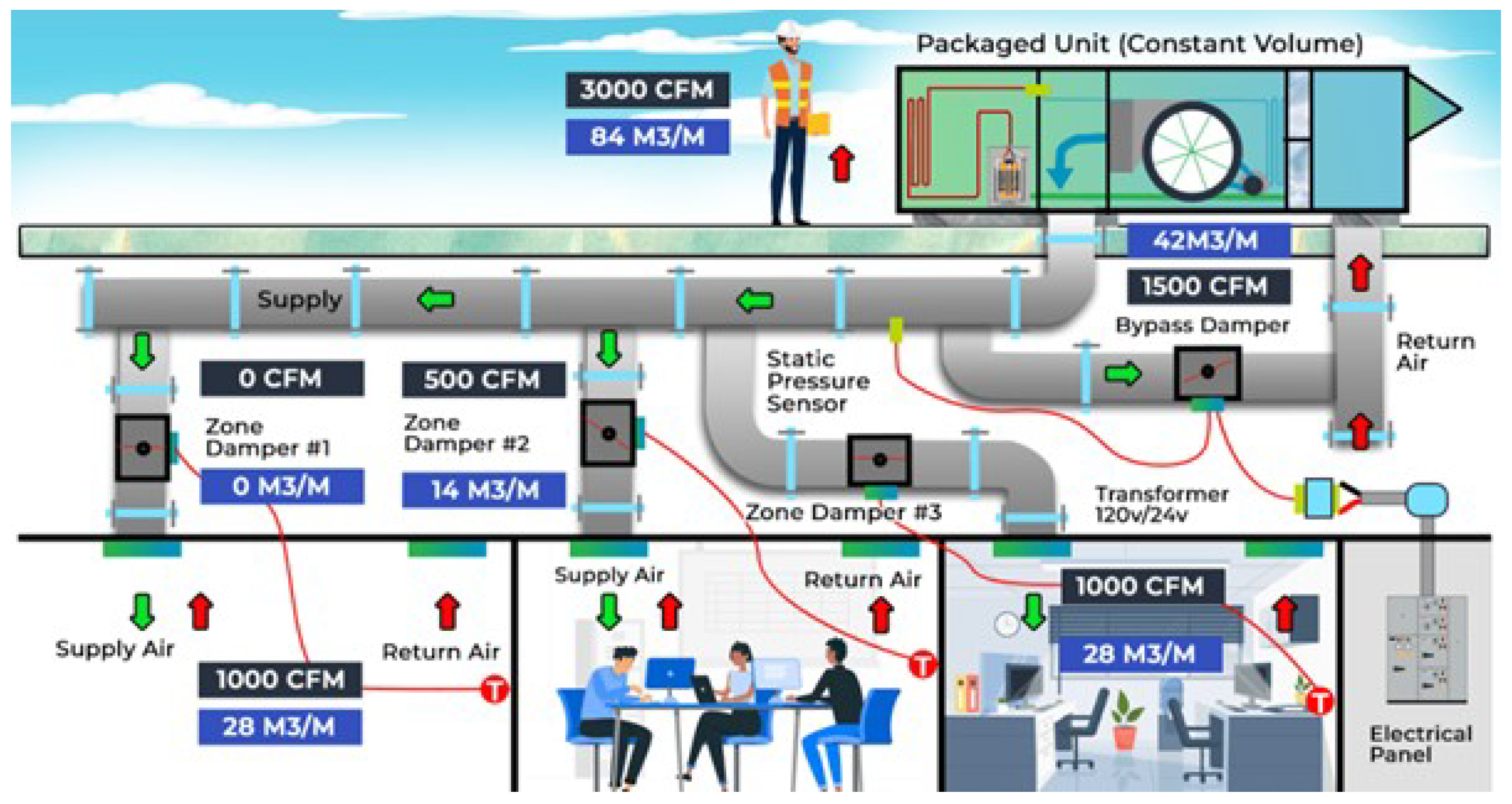
Figure 2.
Thermal Comfort in Commercial Buildings.
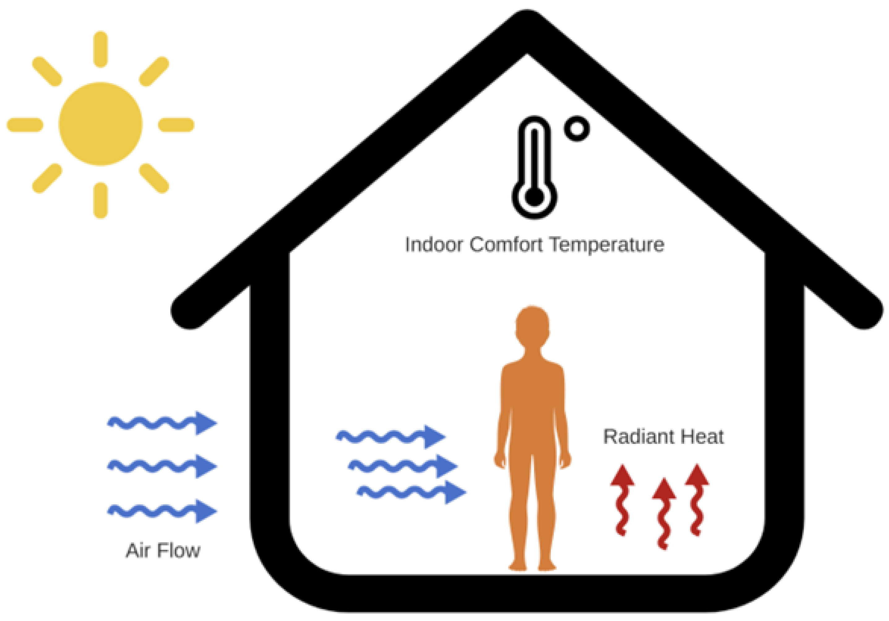
Figure 3.
Proposed Design of a Predictive Model for HVAC Control System.
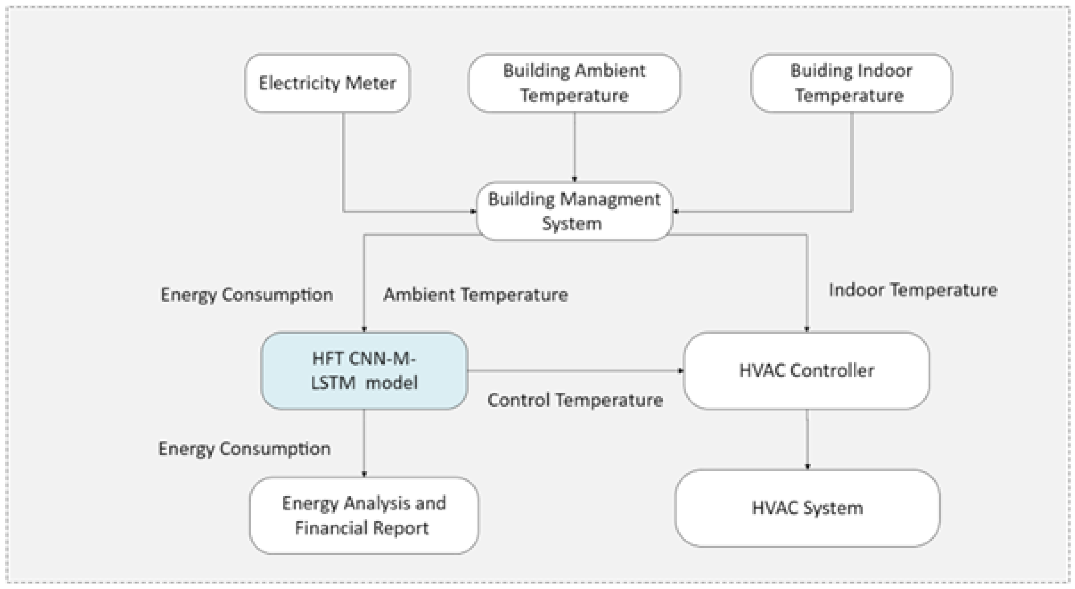
Figure 4.
Correlation Heatmap of Dataset S1 and S2
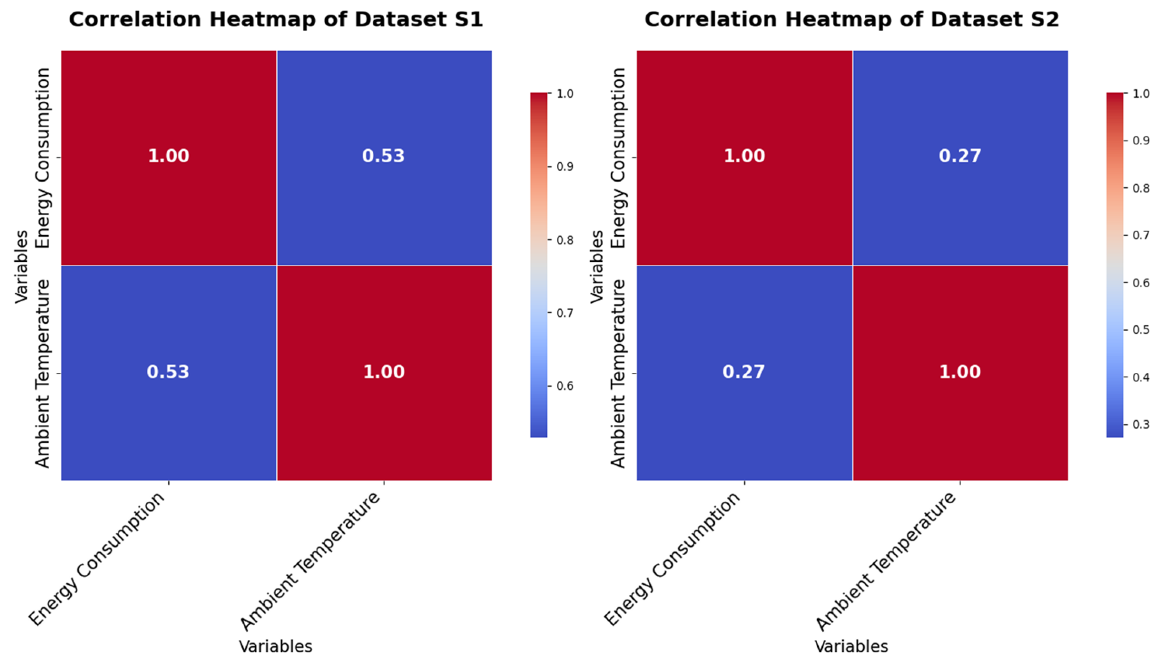
Figure 5.
Location of all the datasets: a. Dataset S1 and S2 location and b. Dataset S3 and S4 location.
Figure 5.
Location of all the datasets: a. Dataset S1 and S2 location and b. Dataset S3 and S4 location.
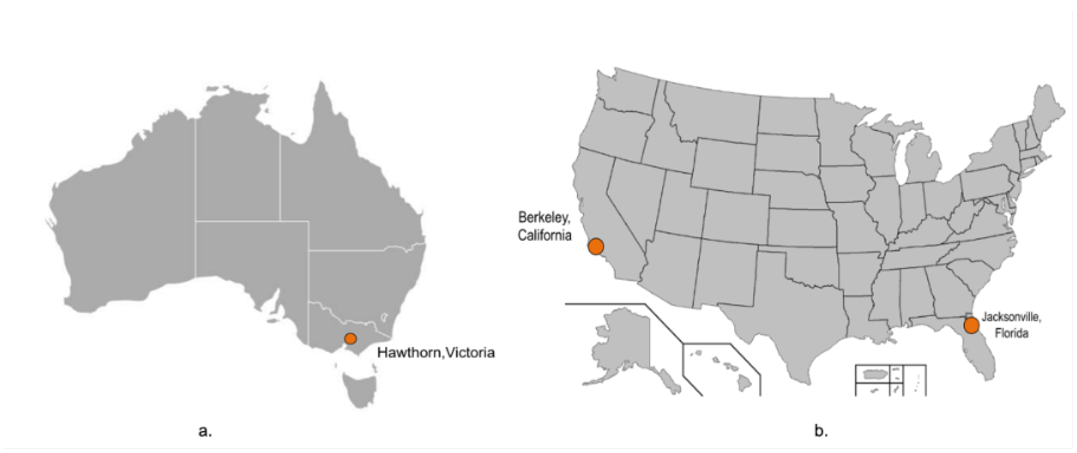
Figure 6.
Location of all the datasets: a. Dataset S1 and S2 location and b. Dataset S3 and S4 location.
Figure 6.
Location of all the datasets: a. Dataset S1 and S2 location and b. Dataset S3 and S4 location.
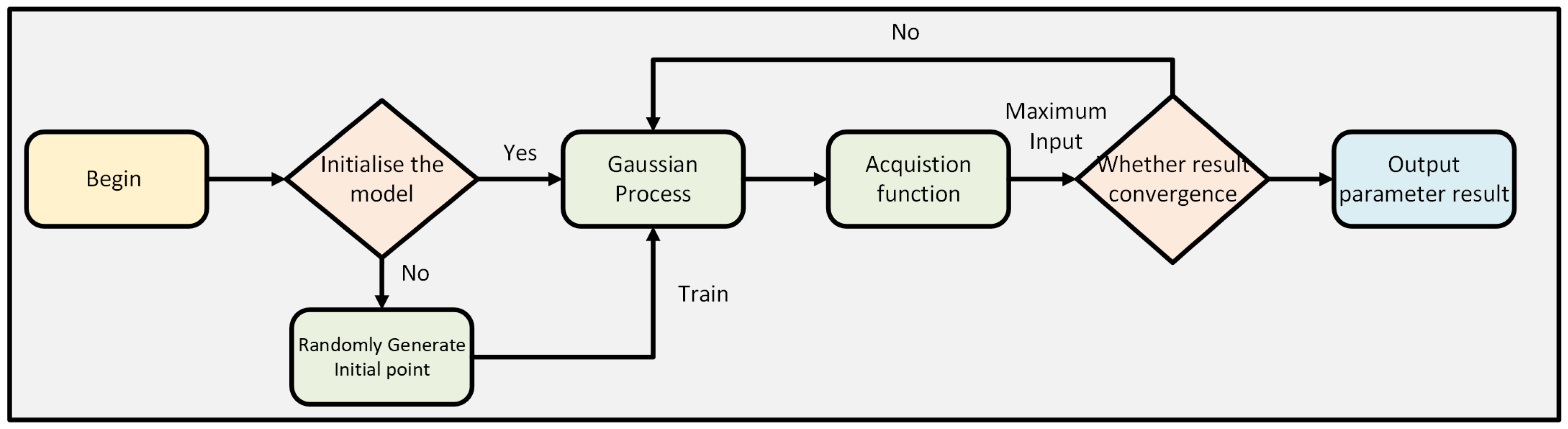
Figure 7.
BO CNN-M-LSTM architecture.
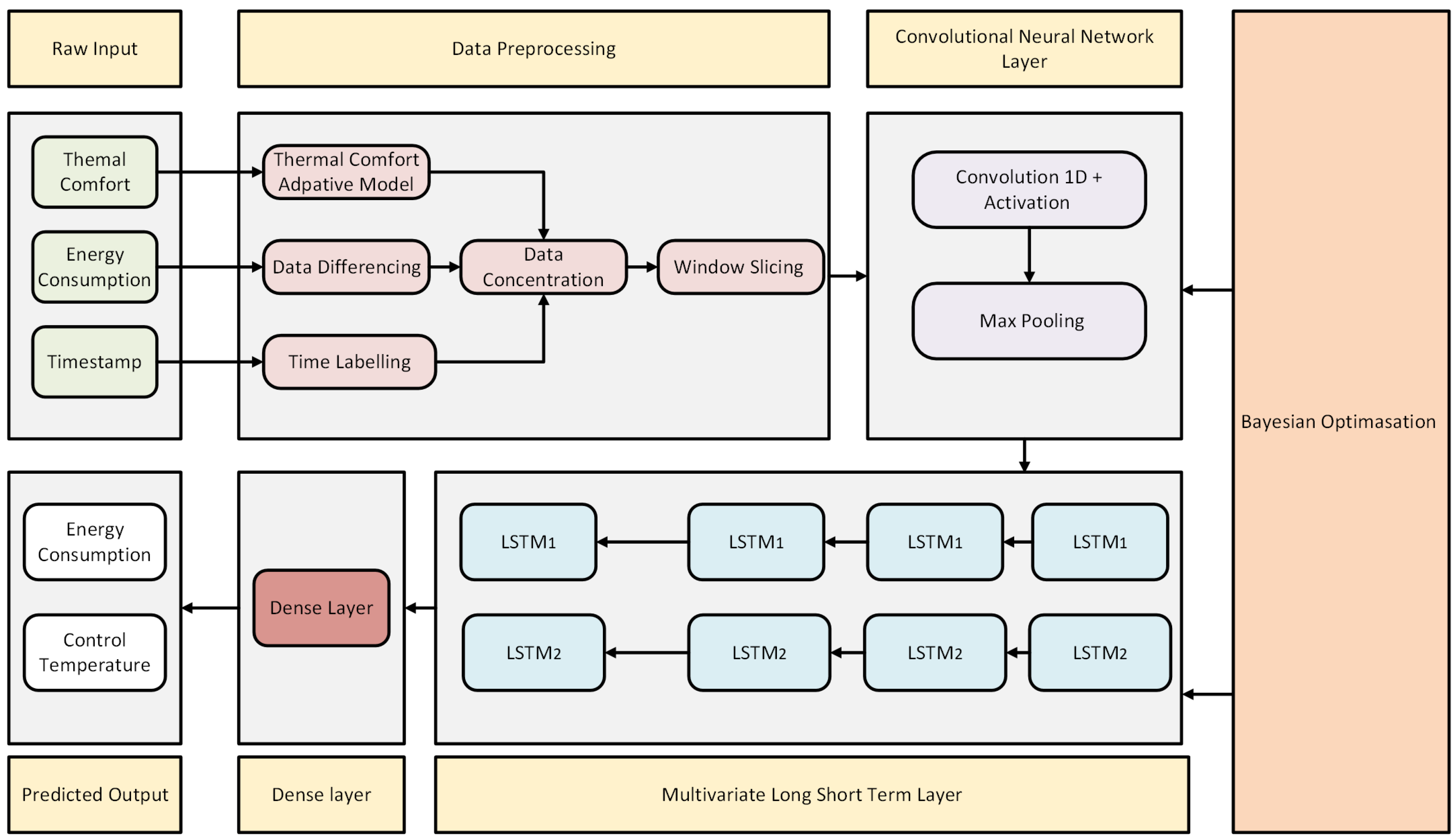
Figure 8.
LSTM cell architecture.
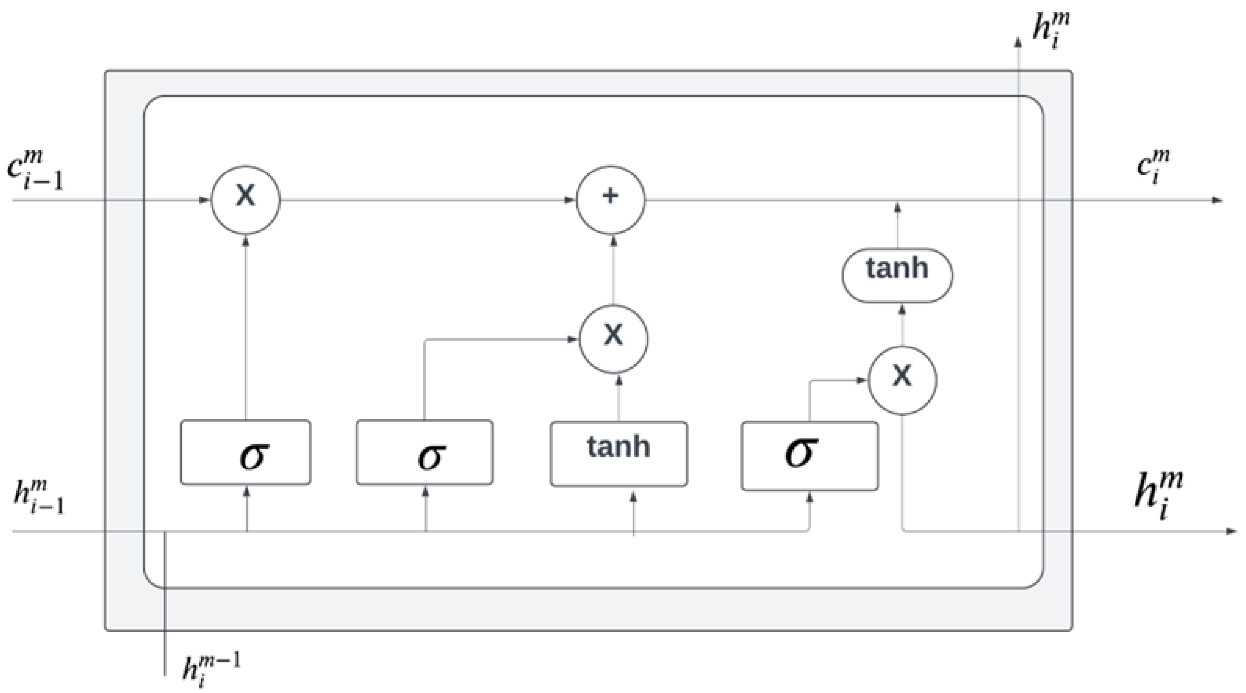
Figure 9.
The performance evaluation of different datasets.
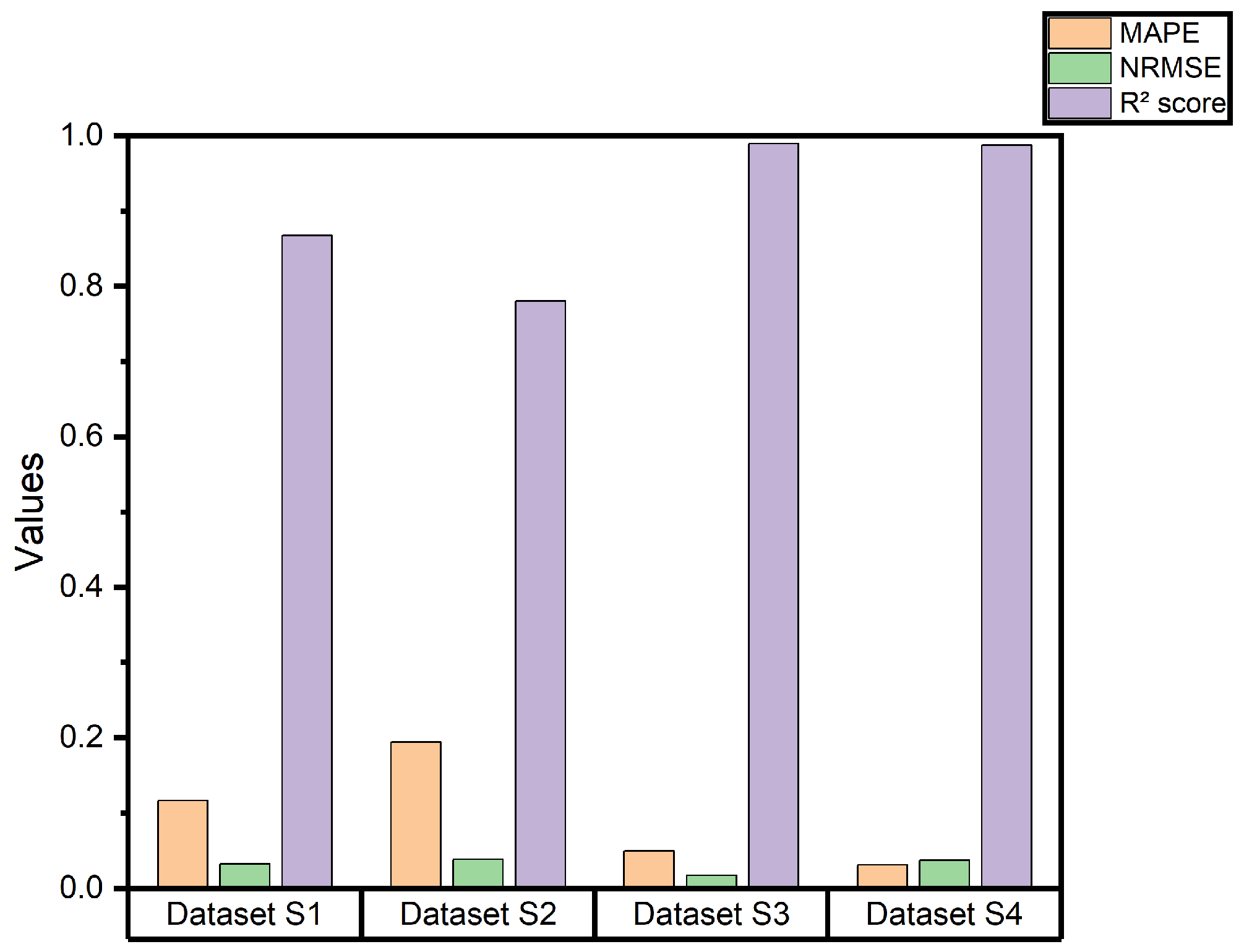
Figure 10.
Prediction for energy consumption of all models for Dataset S1.
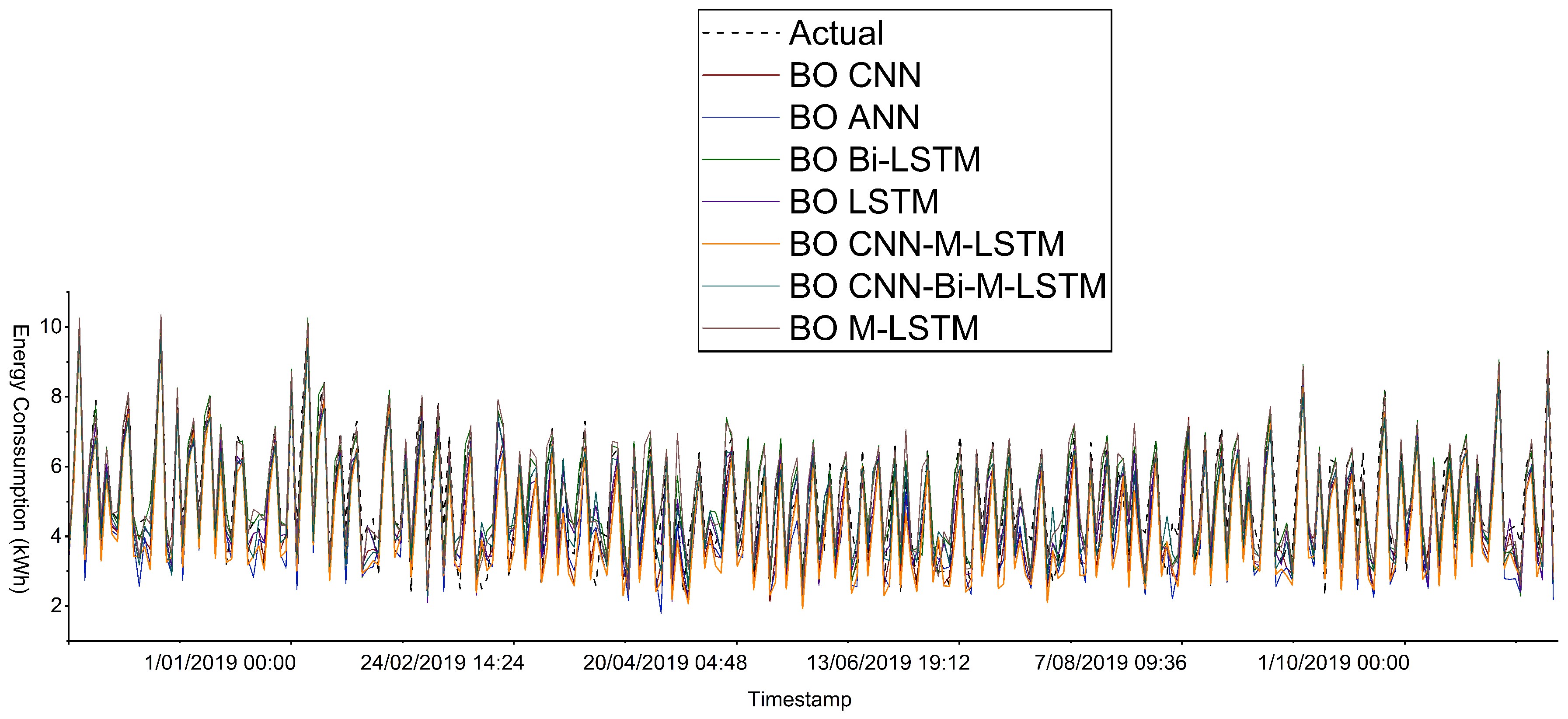
Figure 11.
Prediction for enrgy consumption of all models for Dataset S2.
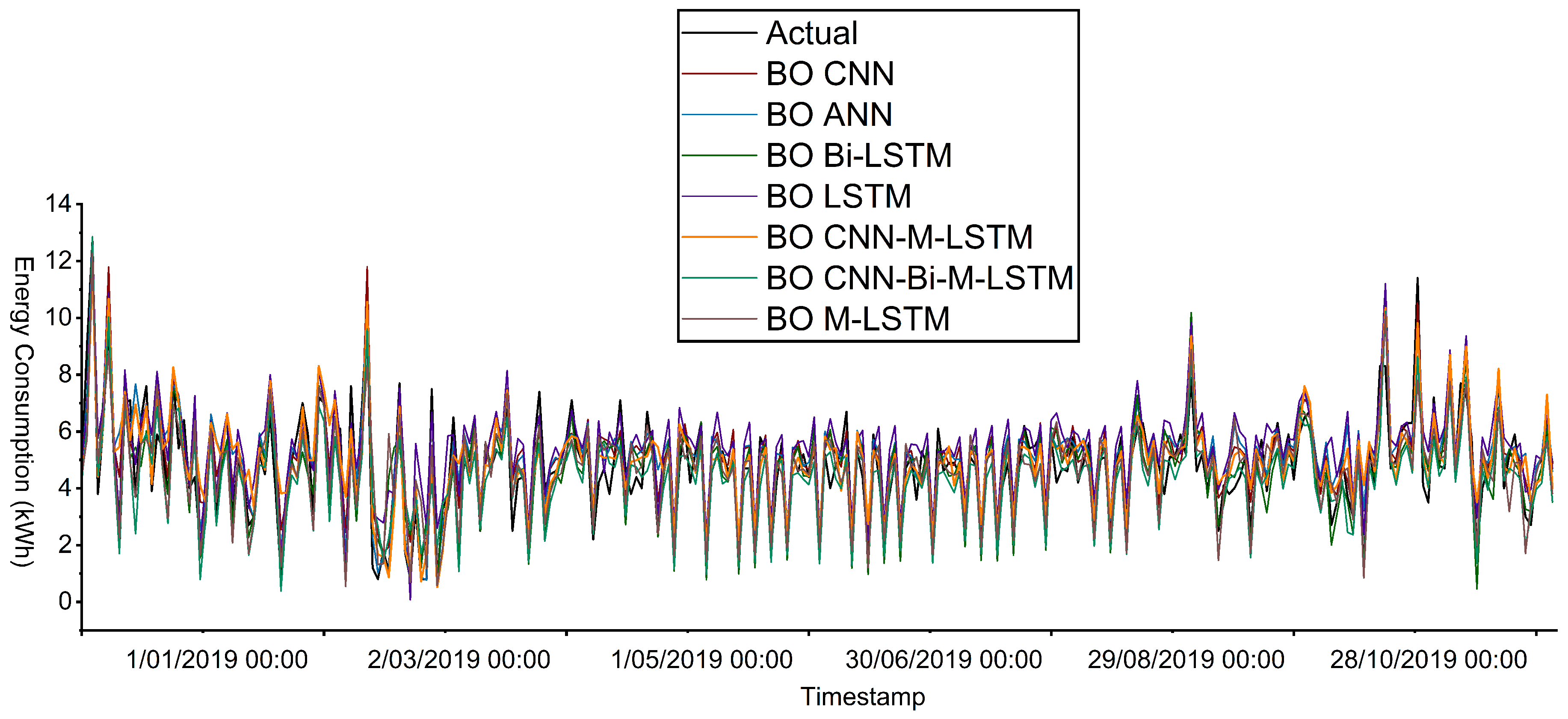
Figure 12.
Prediction for energy consumption of all models for Dataset S3.
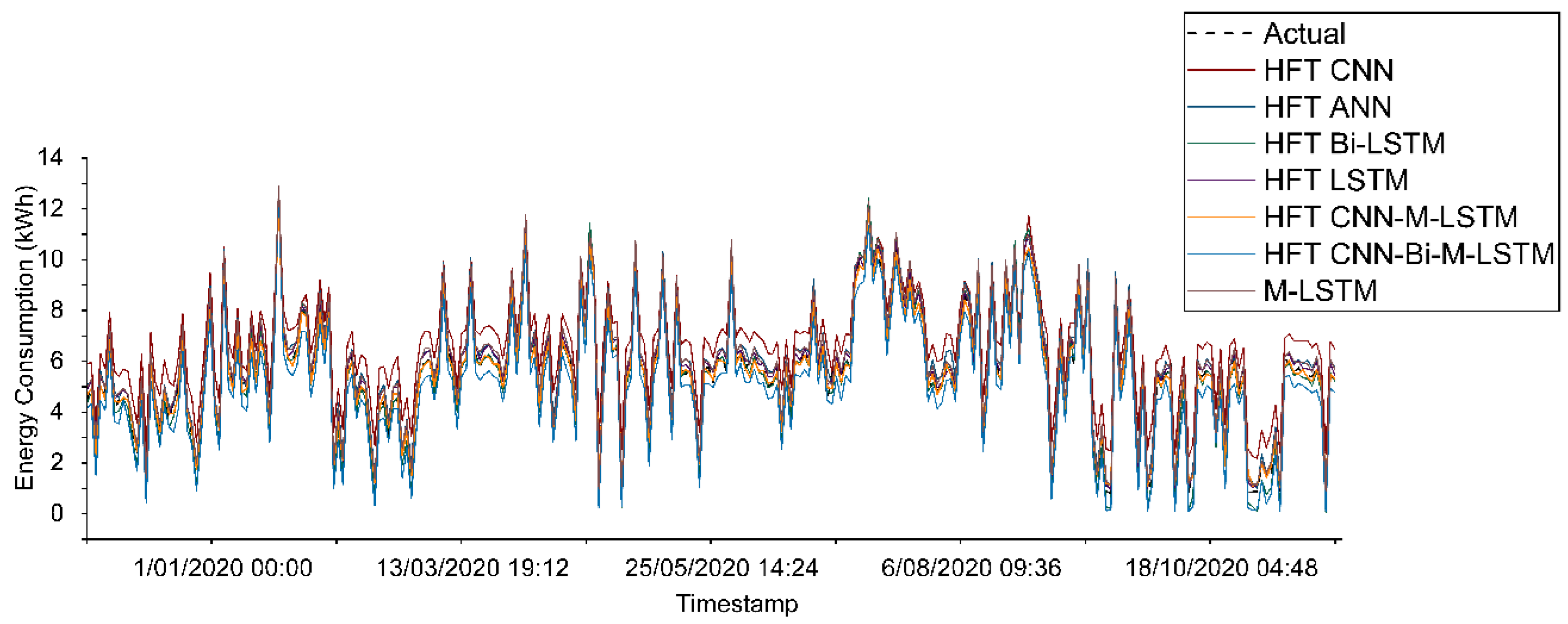
Figure 13.
Prediction for energy consumption of all models for Dataset S4.
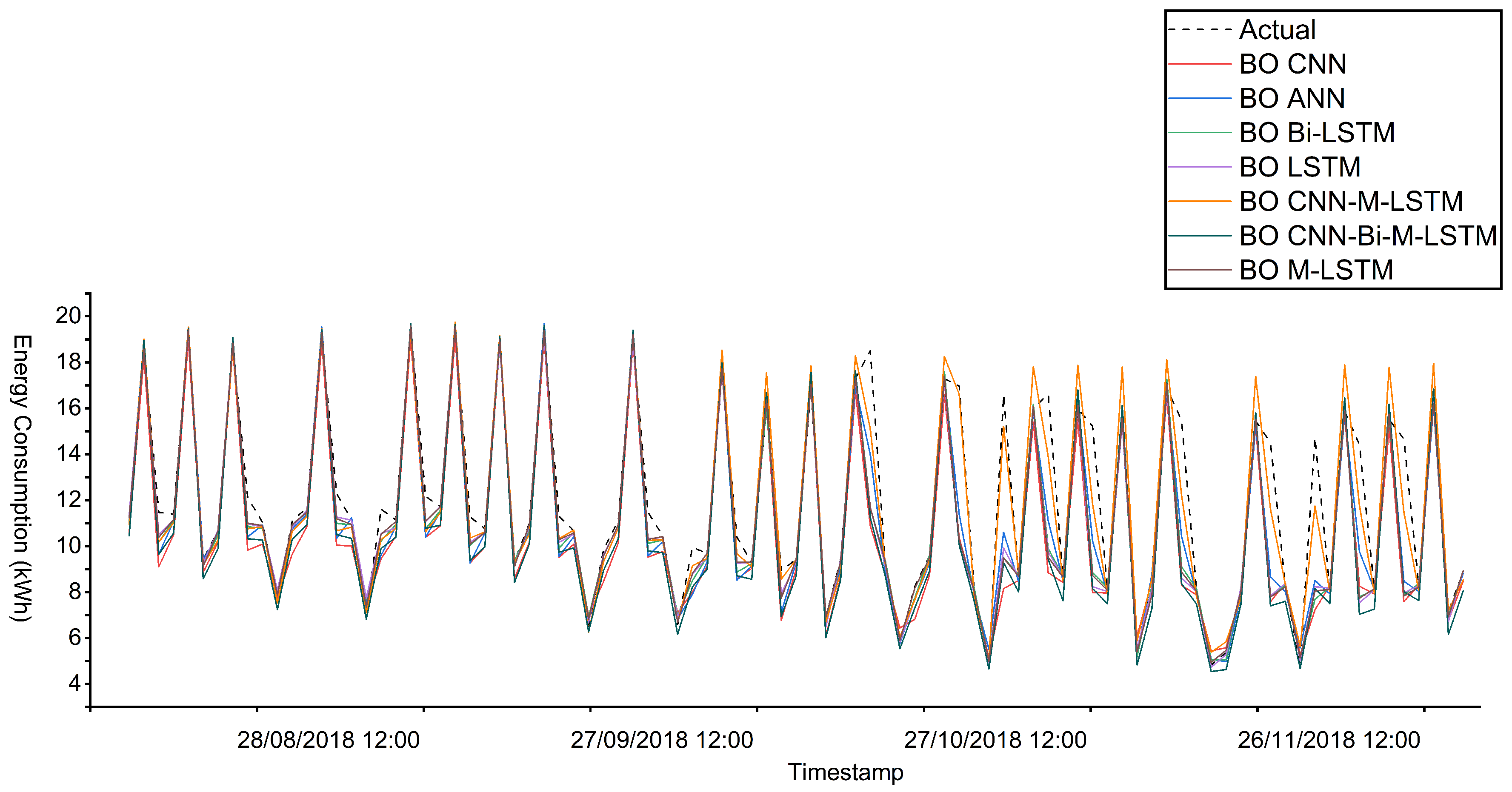
Figure 14.
Prediction energy consumption and control temperature of BO CNN-M-LSTM for Dataset S1.
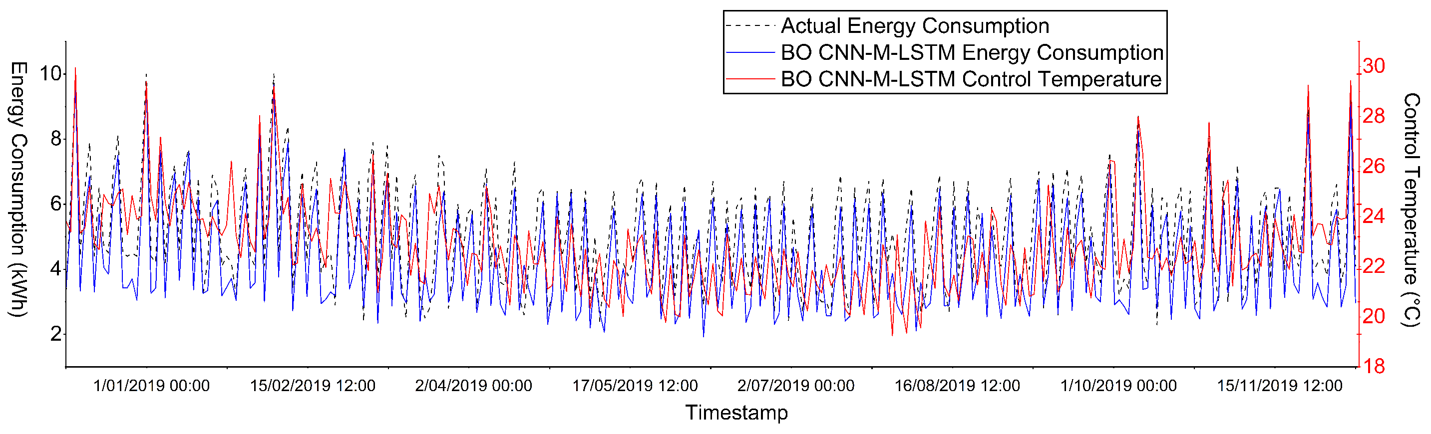
Figure 15.
Prediction energy consumption of BO CNN-M-LSTM for Dataset S1.
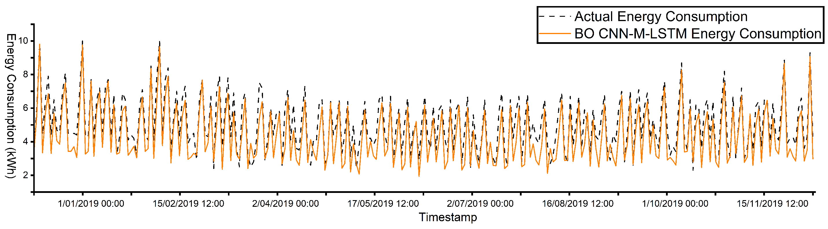
Figure 16.
Prediction energy consumption and control temperature of BO CNN-M-LSTM for Dataset S3.
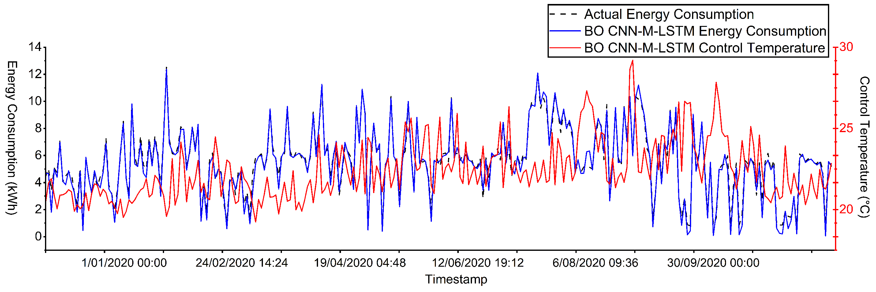
Figure 17.
Prediction energy consumption of BO CNN-M-LSTM for Dataset S3.
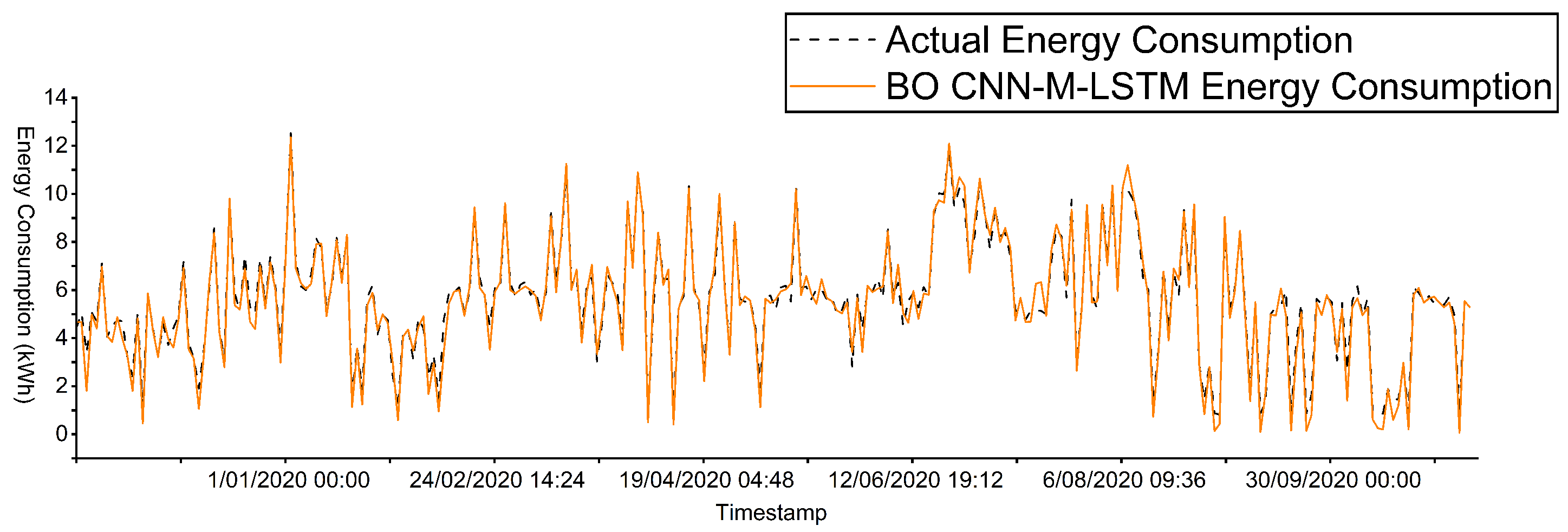
Figure 18.
Metrics result of BO CNN-M-LSTM, BO M-LSTM and BO Bi-LSTM for: a. Dataset S3 and b. Dataset S4.
Figure 18.
Metrics result of BO CNN-M-LSTM, BO M-LSTM and BO Bi-LSTM for: a. Dataset S3 and b. Dataset S4.
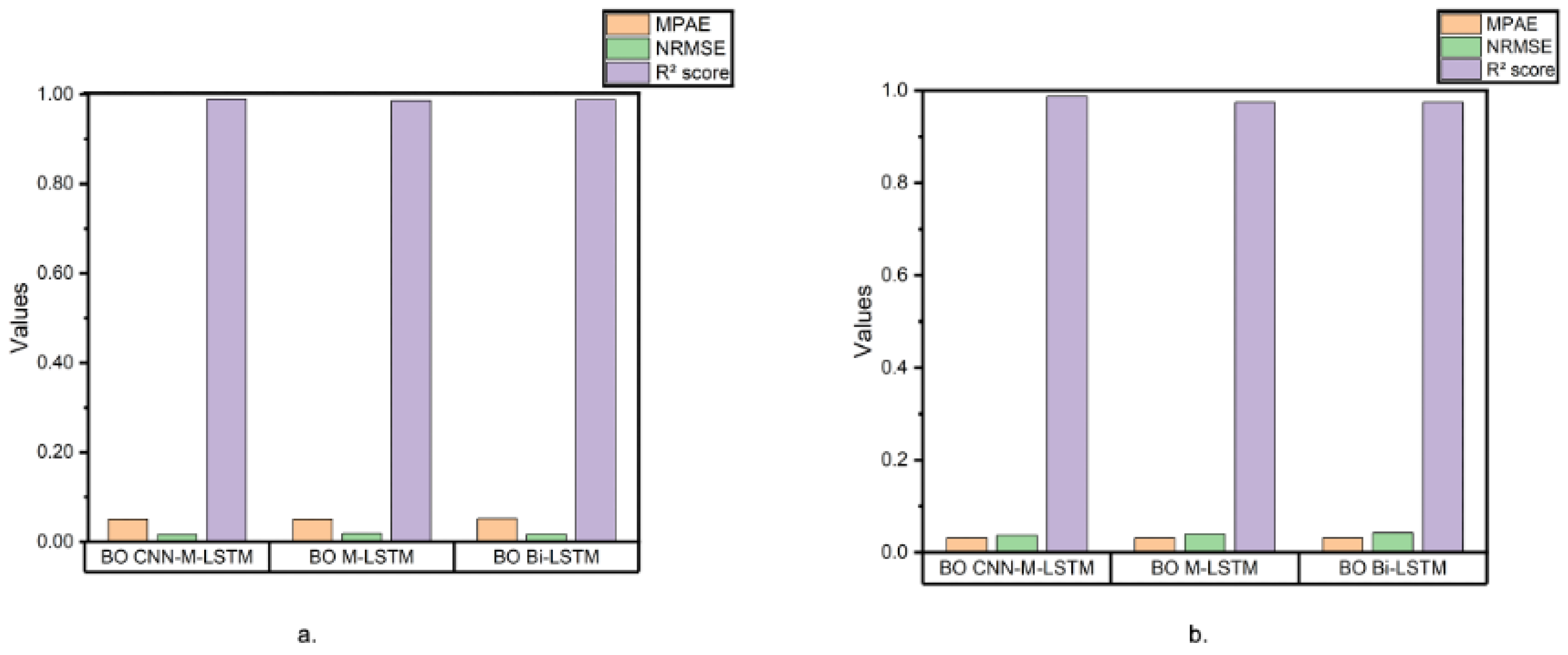

Table 1.
Overview of various models for electricity consumption forecasting of HVAC systems in commercial buildings.
Table 1.
Overview of various models for electricity consumption forecasting of HVAC systems in commercial buildings.
| ID | Forecasting Model | Year | Forecasting Horizon | RMSE | MAE | Score |
| 1 | SVM [10] | 2024 | 10 min ahead | 35,189 W | 25,653 W | 0.930 |
| 2 | ANN [10] | 2024 | 10 min ahead | 24,704 W | 18,081 W | 0.966 |
| 3 | XGBoost [10] | 2024 | 10 min ahead | 16,149 W | 11,354 W | 0.978 |
| 4 | LightGBM [10] | 2024 | 10 min ahead | 24,218 W | 15,827 W | 0.967 |
| 5 | DDPG [11] | 2019 | 5 min ahead | 19.092% | 3.858% | 0.992 |
| 6 | AE–DDPG [11] | 2019 | 5 min ahead | 15.321% | 3.470% | 0.992 |
| 7 | ED-LSTM with MP [12] | 2017 | 83 days ahead | 15.400% | ||
| 8 | ED-LSTM with SMP [12] | 2017 | 83 days ahead | 11.200% |
Table 2.
Model Performance Metrics for Different Datasets
| Dataset | Model | Metrics | Values | ||
| MPAE | NRMSE | score | |||
| Dataset S1 | BO CNN-M-LSTM | 0.1163 | 0.0322 | 0.8676 | |
| BO CNN | 0.1259 | 0.0398 | 0.8551 | ||
| BO ANN | 0.1177 | 0.0365 | 0.8625 | ||
| BO M-LSTM | 0.1248 | 0.0408 | 0.8478 | ||
| BO LSTM | 0.1324 | 0.0429 | 0.8315 | ||
| BO CNN-Bi-M-LSTM | 0.1244 | 0.0404 | 0.8505 | ||
| BO Bi-LSTM | 0.1176 | 0.0388 | 0.8625 | ||
| Dataset S2 | BO CNN-M-LSTM | 0.1939 | 0.0385 | 0.7805 | |
| BO CNN | 0.2744 | 0.0427 | 0.7297 | ||
| BO ANN | 0.1964 | 0.0339 | 0.7788 | ||
| BO M-LSTM | 0.2052 | 0.0420 | 0.7376 | ||
| BO LSTM | 0.2256 | 0.0419 | 0.7388 | ||
| BO CNN-Bi-M-LSTM | 0.1946 | 0.0394 | 0.7692 | ||
| BO Bi-LSTM | 0.1964 | 0.0386 | 0.7788 | ||
| Dataset S3 | BO CNN-M-LSTM | 0.0499 | 0.0166 | 0.9896 | |
| BO CNN | 0.1002 | 0.0449 | 0.9221 | ||
| BO ANN | 0.0510 | 0.0232 | 0.9880 | ||
| BO M-LSTM | 0.0500 | 0.0189 | 0.9861 | ||
| BO LSTM | 0.0570 | 0.0245 | 0.9768 | ||
| BO CNN-Bi-M-LSTM | 0.0579 | 0.0224 | 0.9806 | ||
| BO Bi-LSTM | 0.0511 | 0.0170 | 0.9880 | ||
| Dataset S4 | BO CNN-M-LSTM | 0.0311 | 0.0370 | 0.9872 | |
| BO CNN | 0.0673 | 0.0536 | 0.9590 | ||
| BO ANN | 0.0313 | 0.0399 | 0.9739 | ||
| BO M-LSTM | 0.0371 | 0.0471 | 0.9684 | ||
| BO LSTM | 0.0390 | 0.0494 | 0.9652 | ||
| BO CNN-Bi-M-LSTM | 0.0399 | 0.0380 | 0.9794 | ||
| BO Bi-LSTM | 0.0313 | 0.0428 | 0.9739 | ||
Disclaimer/Publisher’s Note: The statements, opinions and data contained in all publications are solely those of the individual author(s) and contributor(s) and not of MDPI and/or the editor(s). MDPI and/or the editor(s) disclaim responsibility for any injury to people or property resulting from any ideas, methods, instructions or products referred to in the content. |
© 2025 by the authors. Licensee MDPI, Basel, Switzerland. This article is an open access article distributed under the terms and conditions of the Creative Commons Attribution (CC BY) license (http://creativecommons.org/licenses/by/4.0/).
Copyright: This open access article is published under a Creative Commons CC BY 4.0 license, which permit the free download, distribution, and reuse, provided that the author and preprint are cited in any reuse.


