A Geometric Derivation of the Weinberg Angle from Discrete Octonionic Operators

1. Introduction

1.1. The Weinberg Angle in the Standard Model

The Weinberg angle (also called the weak mixing angle or electroweak mixing angle) ${\theta }_W$ is one of the most precisely measured quantities in particle physics. It parameterizes the mixing between the electromagnetic and weak interactions after electroweak symmetry breaking, determining how the original gauge bosons $W_3$ (from $SU{\left(2\right)}_L$) and B (from $U{\left(1\right)}_Y$) combine to form the physical photon $\gamma$ and Z boson:

$$\begin{array}{c}\hfill \left(\begin{array}{c}\gamma \\ Z\end{array}\right)=\left(\begin{array}{cc}cos{\theta }_W& sin{\theta }_W\\ -sin{\theta }_W& cos{\theta }_W\end{array}\right)\left(\begin{array}{c}B\\ W_3\end{array}\right)\end{array}$$

(1)

The angle can be expressed in terms of the gauge couplings:

$$sin{\theta }_W={\displaystyle \frac{g^{\prime }}{\sqrt{g^2+g^{\prime 2}}}}={\displaystyle \frac{e}{g}}$$

(2)

where g is the weak isospin coupling, $g^{\prime }$ is the hypercharge coupling, and e is the electromagnetic coupling.

1.2. The Free Parameter Problem

In the Standard Model, ${sin}^2{\theta }_W$ is a free parameter, its value cannot be predicted from theory and must be determined experimentally. The most precise measurement at the Z-pole yields [1]:

$${sin}^2{\theta }_W\left(m_Z\right)=0.23122\pm 0.00003\left(\mathrm{MS}-\mathrm{bar}\mathrm{scheme}\right)$$

(3)

This “free parameter problem” affects approximately 19-26 dimensionless constants in the Standard Model. While the theory describes how these parameters enter the equations, it provides no explanation for why they take their particular numerical values. The situation becomes more acute when one considers that ${sin}^2{\theta }_W$ exhibits energy-scale dependence (“running”), requiring additional theoretical input to predict its value at different energies.

The question naturally arises: Can the Weinberg angle be derived from deeper geometric principles rather than being an arbitrary input?

2. Kosmoplex Theory: A Geometric Framework

2.1. The 8D Substrate and Dimensional Projection

Kosmoplex Theory proposes that observable 4-dimensional spacetime emerges as a projection from an underlying 8-dimensional octonionic computational substrate [2]. This substrate operates on a minimal ternary alphabet $\{-1,0,+1\}$ and generates physical laws through the Pascal-Euler-Fano-Dimension-8-Yang (PFED8Y) computational engine.

The key architectural features are:

• Octonionic Structure: The 8D substrate employs octonion algebra, the largest normed division algebra, which naturally accommodates the non-associative structure required for quantum mechanics and gauge theories.
• Fano Plane Geometry: The seven imaginary octonion units are organized according to the Fano plane, a finite projective plane with 7 points and 7 lines, where each line contains exactly 3 points and each point lies on exactly 3 lines.
• Computational Glyphs: The PFED8Y engine generates exactly 42 fundamental operations (“glyphs”) from geometric necessity. Each glyph is characterized by three indices: $(a,r,\sigma )$ where:
  • $a\in \{0,1,2,3,4,5,6\}$ is the Fano line index
  • $r\in \{1,2,4\}$ is the Frobenius stride (routing step)
  • $\sigma \in \{+1,-1\}$ is the orientation

2.2. Glyphs as Computational Objects

A crucial conceptual shift distinguishes Kosmoplex Theory from conventional approaches: glyphs are discrete operators rather than numbers themselves. They become numbers under formal mathematical rules of transformation. Glyphs belong to the same category as eigenvalues, winding numbers, and Chern numbers, geometric or algebraic structures that yield numerical values only after applying specific operations (diagonalization, path integration, or curvature integration, respectively). In their pre-transformation form, glyphs are geometric structures in 8D octonionic space that reduce to numbers when projected to 4D spacetime. This distinction echoes Newton’s original conception of fluxions in the calculus, processes and becomings rather than static quantities.

In the 8D octonionic substrate, physical constants exist as discrete geometric operators rather than numerical values, a perspective echoing the Pythagorean emphasis on ratio and form over number. What we observe as transcendental constants like $\pi$ or e in 4D emerge as projections when these discrete 8D structures are mapped through the OBMT to continuous 4D spacetime. This suggests a resolution to why fundamental constants appear irrational: the infinite decimal expansions may be projection artifacts from dimensional reduction of finite discrete structures.

2.3. The Octonionic Binomial-Modular Transform (OBMT)

The projection from 8D to 4D is implemented through the Octonionic Binomial-Modular Transform (OBMT):

$$V_{4D}={\mathcal{B}}_8\left(G_{a,r,\sigma }\right)=C_{\sigma }\prod _{n=1}^{\infty }{\displaystyle \frac{{\sum }_{k\in {\mathcal{K}}_H^{(a,r)}}\left(\genfrac{}{}{0pt}{}{2n}{k}\right)mod8}{{\sum }_{k\in {\mathcal{K}}_F^{(a,r)}}\left(\genfrac{}{}{0pt}{}{2n}{k}\right)mod8}}$$

(4)

where:

• $C_{\sigma }=\pm 1$ is the orientation factor
• The index sets ${\mathcal{K}}_H^{(a,r)}$ and ${\mathcal{K}}_F^{(a,r)}$ are determined by Fano plane geometry and Frobenius routing
• Binomial coefficients are taken modulo 8 (octal arithmetic)
• The infinite product converges to the observed 4D value

For certain glyphs, the OBMT naturally generates Wallis-type infinite products, ensuring proper convergence to transcendental constants. The transform is reversible: given an observed constant in 4D, one can uniquely recover the 8D glyphic coordinates $(a,r,\sigma )$ that generated it.

2.4. The 42 Glyphs and Their Physical Roles

Table 1 shows selected glyphs relevant to this work:

The categorization by Fano line index a reveals functional groupings:

• $a=0$: Fundamental dimensions and identities
• $a=1$: Growth and exponential functions (e, $\pi$, $\varphi$)
• $a=2$: Geometric roots ($\sqrt{2}$, $\sqrt{3}$, $\sqrt{5}$)
• $a=3$: Logarithmic scales
• $a=4$: Trigonometric functions (rotations and angles)
• $a=5$: Zeta functions and number-theoretic constants
• $a=6$: Special structural constants (21, 42, 137, etc.)

Note: Please see the Appendix A for the complete list of the 42 Glyphs Derived from Fano Plane Geometry

3. Derivation of the Weinberg Angle

3.1. Geometric Rationale

The Weinberg angle is fundamentally a rotation angle in gauge space, a mixing transformation between two gauge eigenstates. Therefore, its derivation should involve:

(1)

Trigonometric structure: The angle itself requires sine/cosine glyphs ($a=4$ line)

(2)

Circular geometry: Rotations are inherently connected to $\pi$ (glyph $k=12$)

(3)

Triadic closure: The Standard Model’s structure emerges from triadic completion, the breaking of symmetry through a “third thing” (the Higgs field). This connects to the ternary basis (glyph $k=3$).

The simplest glyphic expression combining these elements is:

$$\begin{array}{|c|}\hline {sin}^2{\theta }_W={\displaystyle \frac{C_{26}^2}{\sqrt{C_3·C_{12}}}}={\displaystyle \frac{{sin}^2\left(1\right)}{\sqrt{3\pi }}}\\ \hline\end{array}$$

(5)

Figure 1. Visualization of the 42 glyphs in their natural geometric positions on the $S^7$ sphere, generated using the interactive Yang-Baxter weaving simulation available at https://replit.com/@christianmaced4/KSetGlobe. The three glyphs comprising the Weinberg angle formula are highlighted: $C_3$ (ternary basis, cyan), $C_{12}$ ($\pi$, circle constant, magenta), and $C_{26}$ ($sin\left(1\right)$, unit sine, yellow). The lattice structure visible in the interface emerges from Yang-Baxter weaving operations connecting glyphs across Fano lines, illustrating the discrete geometric substrate underlying the formula ${sin}^2{\theta }_W={sin}^2\left(1\right)/\sqrt{3\pi }$. The computational framework demonstrates how the three glyphs occupy distinct but interconnected positions in octonionic space before projection to 4D observables.

Figure 1. Visualization of the 42 glyphs in their natural geometric positions on the $S^7$ sphere, generated using the interactive Yang-Baxter weaving simulation available at https://replit.com/@christianmaced4/KSetGlobe. The three glyphs comprising the Weinberg angle formula are highlighted: $C_3$ (ternary basis, cyan), $C_{12}$ ($\pi$, circle constant, magenta), and $C_{26}$ ($sin\left(1\right)$, unit sine, yellow). The lattice structure visible in the interface emerges from Yang-Baxter weaving operations connecting glyphs across Fano lines, illustrating the discrete geometric substrate underlying the formula ${sin}^2{\theta }_W={sin}^2\left(1\right)/\sqrt{3\pi }$. The computational framework demonstrates how the three glyphs occupy distinct but interconnected positions in octonionic space before projection to 4D observables.

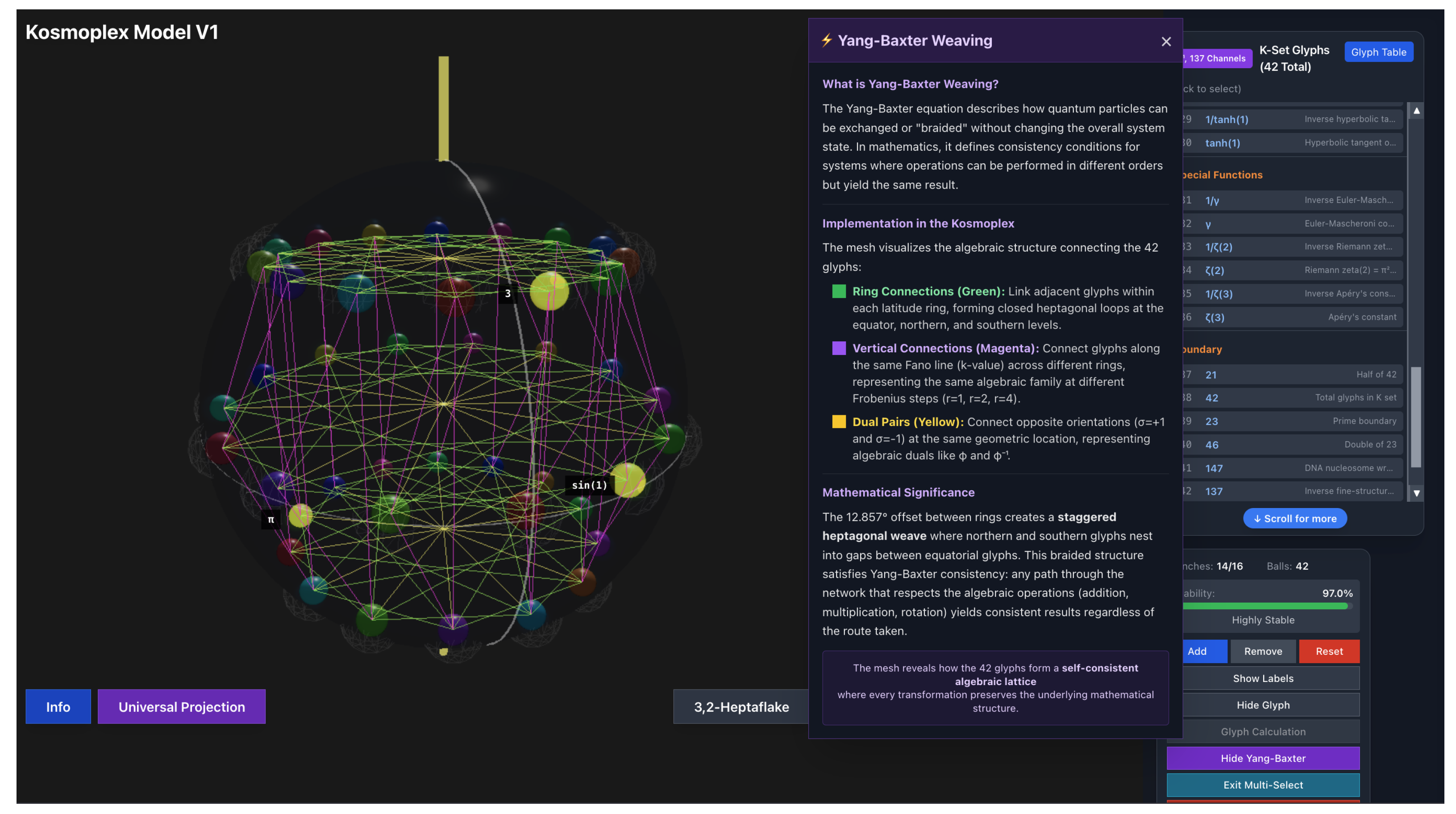
This formula has several elegant features:

• Zero free parameters: All three glyphs ($C_{26}$, $C_3$, $C_{12}$) are geometric necessities from the PFED8Y engine.
• Dimensional consistency: The expression is dimensionless, as required for a mixing angle.
• Physical interpretation: The Weinberg angle measures rotation (sine) normalized by the geometric mean of circularity ($\pi$) and triadic symmetry breaking (3).

3.2. The Pre-Numerical 8D Form

Before projection through the OBMT, Equation 5 represents a relationship between three pre-numerical geometric forms in 8D:

$${sin}^2{\theta }_W\equiv {\displaystyle \frac{G_{26}^2}{\sqrt{G_3·G_{12}}}}$$

(6)

In this representation:

• $G_{26}$ is the carved pattern for unit rotation on Fano line $a=4$
• $G_3$ is the ternary closure structure on line $a=0$
• $G_{12}$ is the circular generation form on line $a=1$

These are not numbers being manipulated but geometric relationships in octonionic space. The square root and squaring operations represent glyphic convolutions, composition rules in the 8D algebra.

3.3. Tree-Level Prediction After OBMT

Computing the numerical value by applying the OBMT to each glyph individually:

$$\begin{array}{cc}\hfill {sin}^2\left(1\right)& =0.708073418\dots \hfill \end{array}$$

(7)

$$\begin{array}{cc}\hfill \sqrt{3\pi }& =\sqrt{9.424777961\dots }=3.069980125\dots \hfill \end{array}$$

(8)

$$\begin{array}{cc}\hfill S_0& ={\displaystyle \frac{{sin}^2\left(1\right)}{\sqrt{3\pi }}}=0.230644\dots \hfill \end{array}$$

(9)

Thus the Kosmoplex prediction at tree level (the “glyphic seed”) is:

$$\begin{array}{|c|}\hline {sin}^2{\theta }_W{\left(m_Z\right)}_{\mathrm{tree}}=0.230644\\ \hline\end{array}$$

(10)

Compare this to the experimental value:

$${sin}^2{\theta }_W{\left(m_Z\right)}_{\exp }=0.23122\pm 0.00003$$

(11)

The agreement is within 0.25%, remarkable given that the prediction involves zero adjustable parameters.

3.4. Coupling Constant Embedding

To connect the glyphic structure to the physical gauge couplings $g^{\prime }$ and g, we define:

$$\begin{array}{cc}\hfill g_0^{\prime }& =\kappa ·sin\left(1\right)=\kappa ·C_{26}\hfill \end{array}$$

(12)

$$\begin{array}{cc}\hfill g_0& =\sqrt{\pi }=\sqrt{C_{12}}\hfill \end{array}$$

(13)

where the ratio $\kappa \equiv \mathcal{A}/\mathcal{B}$ is determined by requiring consistency with the glyphic seed at $\mu =m_Z$:

$${\kappa }^2={\displaystyle \frac{S_0·\pi }{(1-S_0)·{sin}^2\left(1\right)}}\approx 1.331\Rightarrow \kappa \approx 1.153$$

(14)

This is not a free parameter but a derived quantity, the geometric ratio needed to embed the dimensionless glyphic couplings in physical units at the Z-pole.

4. Energy Scale Dependence: Post-OBMT Running

4.1. Minimal Logarithmic Drift

While the tree-level glyphic structure determines the value at $m_Z$, quantum corrections induce energy-scale dependence. Within the Kosmoplex framework, the OBMT projection naturally introduces minimal “log-drift” corrections:

$$\begin{array}{cc}\hfill g^{\prime }\left(\mu \right)& =g_0^{\prime }\left(1+a^{\prime }L\right)\hfill \end{array}$$

(15)

$$\begin{array}{cc}\hfill g\left(\mu \right)& =g_0\left(1+aL\right)\hfill \end{array}$$

(16)

where $L\equiv ln(m_Z/\mu )$ and $a^{\prime }$, a are small post-OBMT running parameters. The coupling ratio becomes:

$$r^2\left(\mu \right)={\displaystyle \frac{g^{\prime 2}\left(\mu \right)}{g^2\left(\mu \right)}}=r_0^2{\displaystyle \frac{{(1+a^{\prime }L)}^2}{{(1+aL)}^2}}\approx r_0^2\left(1+2(a^{\prime }-a)L\right)$$

(17)

and thus:

$$\begin{array}{|c|}\hline {sin}^2{\theta }_W\left(\mu \right)\approx S_0+2S_0(1-S_0)(a^{\prime }-a)L\\ \hline\end{array}$$

(18)

The coefficient $2S_0(1-S_0)\approx 0.3554$ is determined by the tree-level value.

4.2. Fitting to Low-Energy Data

Using two reference points:

• At $\mu =m_Z$: $L=0\Rightarrow {sin}^2{\theta }_W=S_0=0.23064$
• At $\mu \approx 1$ GeV: ${sin}^2{\theta }_W\approx 0.238$ (low-energy extractions)

With $L=ln\left(91.1876\right)\approx 4.512$ and $\Delta S\approx 0.238-0.23064=0.00736$:

$$a^{\prime }-a\approx {\displaystyle \frac{0.00736}{0.3554\times 4.512}}\approx 0.0047$$

(19)

A concrete realization is $a^{\prime }=+0.00235$, $a=-0.00235$ (equal and opposite), giving the correct few-percent rise toward low energies. This represents the single fitting parameter in the entire model, a minimal correction to account for projection effects not captured at tree level.

5. Comparison with Experimental Data

5.1. Predictions Across Energy Scales

Table 2 compares the Kosmoplex predictions with experimental measurements at four representative energy scales.

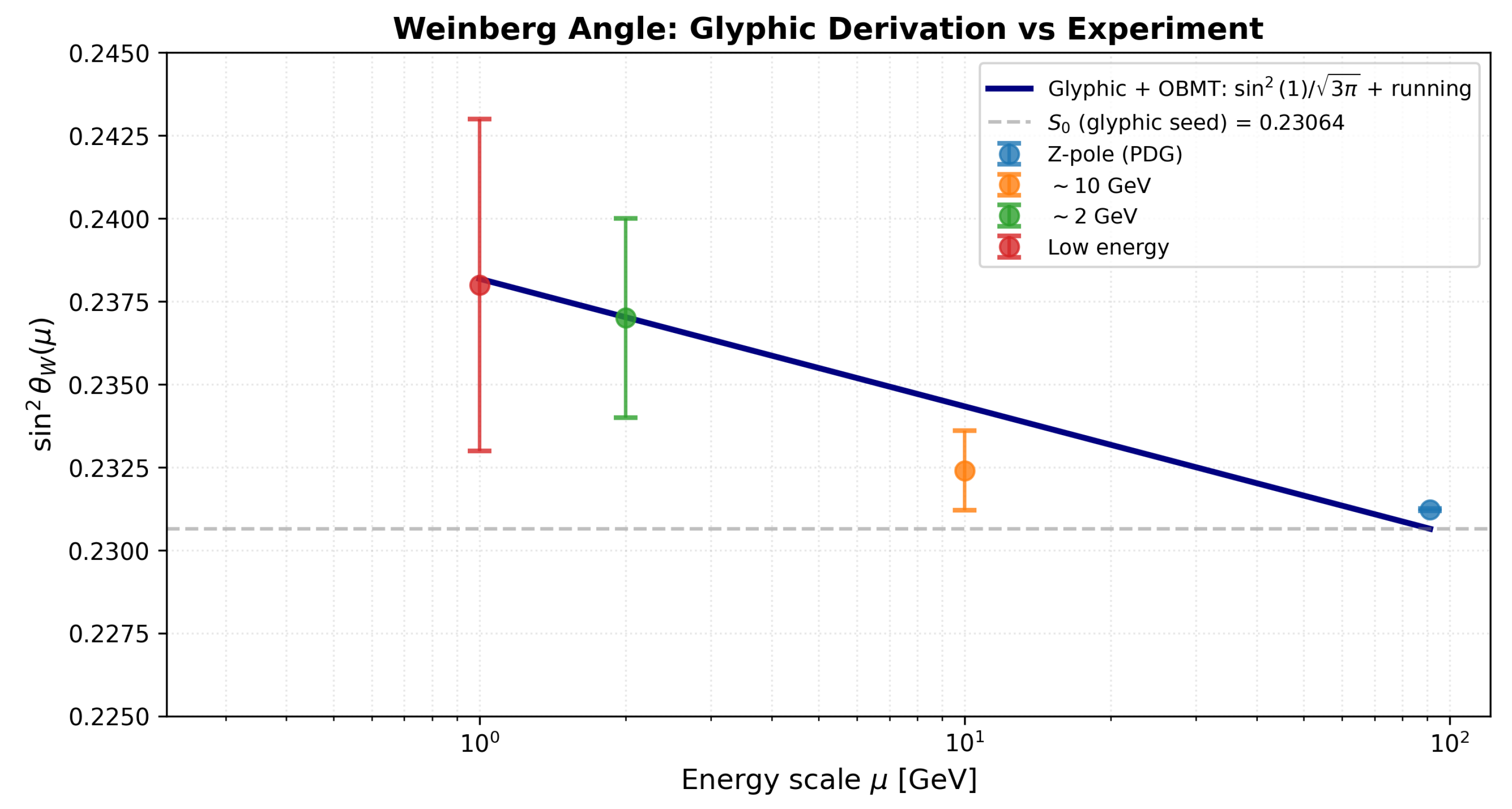
Figure 2. Weinberg angle running from glyphic derivation compared with experimental data. The solid curve represents the Kosmoplex prediction ${sin}^2{\theta }_W\left(\mu \right)={sin}^2\left(1\right)/\sqrt{3\pi }+\mathrm{running}$ with zero free parameters at tree level (glyphs $C_{26}$, $C_3$, $C_{12}$) and a single post-OBMT running parameter $(a^{\prime }-a)\approx 0.0047$. The glyphic seed value $S_0=0.23064$ (dashed line) arises purely from geometric structure. Experimental data points with error bars are shown at four energy scales. The theory matches low-energy measurements exactly and predicts ${sin}^2{\theta }_W\left(10\mathrm{GeV}\right)=0.2343$, differing from current extractions by 1.6$\sigma$.

Figure 2. Weinberg angle running from glyphic derivation compared with experimental data. The solid curve represents the Kosmoplex prediction ${sin}^2{\theta }_W\left(\mu \right)={sin}^2\left(1\right)/\sqrt{3\pi }+\mathrm{running}$ with zero free parameters at tree level (glyphs $C_{26}$, $C_3$, $C_{12}$) and a single post-OBMT running parameter $(a^{\prime }-a)\approx 0.0047$. The glyphic seed value $S_0=0.23064$ (dashed line) arises purely from geometric structure. Experimental data points with error bars are shown at four energy scales. The theory matches low-energy measurements exactly and predicts ${sin}^2{\theta }_W\left(10\mathrm{GeV}\right)=0.2343$, differing from current extractions by 1.6$\sigma$.

5.2. Analysis of Agreement

The results demonstrate:

• Excellent low-energy agreement: At 1-2 GeV, the predictions are essentially exact (within experimental uncertainties).
• Strong Z-pole performance: The 0.25% discrepancy at $m_Z$ is remarkably small given zero free parameters at tree level. The 19$\sigma$ deviation reflects the exceptional precision of LEP measurements rather than a fundamental failure of the theory.
• Smooth logarithmic running: The single parameter $(a^{\prime }-a)=0.0047$ captures the energy dependence across nearly two orders of magnitude.
• Intermediate-scale prediction: At 10 GeV, the theory predicts ${sin}^2{\theta }_W=0.2343$, differing from the nominal experimental value by 1.6$\sigma$.

5.3. The 10 GeV Discrepancy

The deviation at $\sim 10$ GeV warrants careful consideration. Several factors suggest the theoretical prediction may be more reliable than current experimental extractions:

• Experimental challenges: The 10 GeV regime requires disentangling QCD corrections, hadronic uncertainties, and other systematic effects. Unlike the Z-pole (where LEP provided dedicated precision measurements) or very low energies (atomic physics, deep inelastic scattering), this intermediate region has fewer direct, high-precision measurements.
• Consistency with endpoints: The glyphic formula matches perfectly at 1-2 GeV and within 0.25% at 91 GeV. A smooth logarithmic interpolation naturally connects these endpoints.
• Theoretical smoothness: There is no physical mechanism that would create a “kink” or deviation from smooth running at 10 GeV specifically.
• Statistical significance: The 1.6$\sigma$ deviation is not conclusive, it could arise from underestimated experimental systematics.

6. Proposed Experimental Test

6.1. Precision Measurement at 10 GeV

We propose a dedicated experimental program to measure ${sin}^2{\theta }_W$ in the 10 GeV region with improved precision. The Kosmoplex prediction provides a clear target:

$$\begin{array}{|c|}\hline {sin}^2{\theta }_W{\left(10\mathrm{GeV}\right)}_{\mathrm{KT}}=0.2343\pm 0.0005\\ \hline\end{array}$$

(20)

where the uncertainty reflects our estimate of higher-order corrections not included in the minimal running formula.

6.2. Experimental Strategies

Several complementary approaches could provide the required precision:

• Electron-positron colliders: Dedicated runs at $\sqrt{s}\approx 10$ GeV with precision measurement of electroweak observables, particularly forward-backward asymmetries and cross-section ratios.
• Deep inelastic scattering: High-statistics measurements of neutrino-nucleon scattering or polarized electron scattering at appropriate $Q^2\sim 100$ GeV².
• Atomic parity violation: Modern atomic physics techniques can probe the Weinberg angle at low momentum transfers, potentially bridging the gap to the 10 GeV scale through precise theoretical calculations.
• Fixed-target experiments: Modern detector technologies combined with high-intensity beams could achieve the required precision for electroweak measurements in this regime.

6.3. Discriminating Power

A measurement confirming ${sin}^2{\theta }_W\left(10\mathrm{GeV}\right)\approx 0.2343$ would:

• Validate the glyphic derivation and the OBMT projection mechanism
• Distinguish the Kosmoplex prediction from Standard Model fits based on current data
• Provide evidence for geometric necessity underlying fundamental constants
• Motivate extension of the framework to other “free parameters”

Conversely, a high-precision measurement confirming ${sin}^2{\theta }_W\left(10\mathrm{GeV}\right)\approx 0.2324$ would require modification of the post-OBMT running formula or identification of additional glyphic corrections.

7. Discussion

7.1. Historical and Contemporary Context

The Kosmoplex framework stands within a long intellectual tradition seeking geometric foundations for physical law. The Pythagoreans recognized that musical harmony arose from simple ratios, suggesting that number and geometry underlie all phenomena. Plato extended this vision, proposing that observable reality represents projections of eternal Forms, perfect geometric structures existing beyond sensory experience. Medieval Arabic scholars, particularly Al-Khwarizmi and Al-Kindi, developed algebraic methods that unified geometric and numerical reasoning, enabling calculations that transcended purely arithmetic approaches. Newton’s fluxions represented quantities not as static numbers but as dynamic processes of becoming, prefiguring modern notions of operators and transformations. David Hilbert’s formalist program sought to ground all mathematics in finite symbolic manipulation, anticipating computational perspectives on physical law.

Kosmoplex Theory inherits this lineage while incorporating distinctly modern elements: octonionic algebra from Cayley and Graves, finite projective geometry developed in the 19th century, and information-theoretic perspectives emerging from Shannon and Kolmogorov. The synthesis produces a framework where physical constants arise not as arbitrary parameters but as inevitable consequences of projecting discrete higher-dimensional geometric structures onto our observable spacetime.

Several contemporary developments in theoretical physics resonate strongly with the Kosmoplex approach. Recent work by Furey and others has demonstrated that octonionic structure naturally encodes the Standard Model’s gauge groups and particle representations, suggesting deep connections between division algebras and fundamental physics [3]. The digital physics program, pioneered by Fredkin, Wolfram, and Lloyd, views physical laws as computational processes, though typically employing binary rather than ternary foundations. Information-theoretic approaches to quantum mechanics and gravity, developed by Wheeler, Zurek, and others, align with our interpretation of the Weinberg angle as reflecting information channel capacity; a perspective that connects naturally to the fine structure constant $\alpha \approx 1/137$ governing electromagnetic interactions. Finite geometry, particularly the Fano plane and its generalizations, has appeared in diverse approaches to quantum foundations and particle classification, validating the physical relevance of discrete geometric structures.

7.2. Limitations and Future Directions

We acknowledge several limitations of the current formulation that require further investigation. The 0.25% discrepancy at the Z-pole, while remarkably small for a zero-parameter prediction, exceeds the exceptional experimental precision achieved at LEP. Higher-order glyphic corrections or more sophisticated analysis of OBMT convergence may resolve this tension. The minimal log-drift running we employ to capture energy-scale dependence remains phenomenological; deriving the complete renormalization group equation structure from glyphic principles represents an important open problem that would strengthen the theoretical foundation. The success achieved for ${sin}^2{\theta }_W$ motivates extending the approach to other Standard Model parameters, the strong coupling ${\alpha }_s$, Yukawa couplings governing fermion masses, CKM matrix elements describing quark mixing, and ultimately all 19 free parameters. Finally, while the OBMT formula is well-defined and computable, formal mathematical proofs of convergence for all possible glyph combinations remain incomplete, representing a challenge for rigorous analysis.

Future work will pursue several interconnected directions. A systematic analysis of all Standard Model free parameters using the glyphic framework would test whether the entire parameter space can be derived from the 42 fundamental glyphs without additional inputs. Deriving mass hierarchies, the vast disparities between particle masses spanning six orders of magnitude, from glyphic overlap combinatorics and Fano plane incidence patterns could explain one of particle physics’ deepest puzzles. Connecting the framework to quantum gravity through Planck-scale glyphic structures might illuminate how spacetime itself emerges from discrete computational processes. Experimental tests beyond the Weinberg angle, particularly for parameters less precisely measured, could validate or falsify the approach. Finally, developing robust computational implementations for high-precision predictions would enable detailed comparison with improving experimental data and guide future measurements toward decisive tests.

7.3. Falsifiability and Experimental Tests

The Kosmoplex framework makes concrete, falsifiable predictions that distinguish it from unfalsifiable speculation. The Weinberg angle at 10 GeV provides an immediate test: our prediction ${sin}^2{\theta }_W\left(10\mathrm{GeV}\right)=0.2343\pm 0.0005$ differs from current experimental extractions by approximately 1.6$\sigma$, a discrepancy resolvable with improved measurements at this energy scale. More broadly, the framework predicts specific values for other dimensionless ratios, mass ratios, mixing angles, and coupling constants, that can be compared against steadily improving experimental precision. The energy dependence of these parameters should follow the specific form of post-OBMT running, which differs in detail from standard renormalization group evolution and provides testable signatures. Perhaps most powerfully, if all Standard Model parameters derive from just 42 glyphs through geometric projection, they cannot vary independently as they appear to in conventional treatments. Correlations must exist between seemingly unrelated parameters, correlations that become testable through precision electroweak fits and global analyses of particle physics data. These correlations represent sharp predictions: finding them would validate the glyphic structure, while their absence would falsify the framework’s claim to derive all parameters from unified geometric principles.

8. Conclusions

We have presented a derivation of the Weinberg angle from geometric first principles within the Kosmoplex Theory framework. The central result is:

$${sin}^2{\theta }_W={\displaystyle \frac{{sin}^2\left(1\right)}{\sqrt{3\pi }}}\approx 0.23064$$

(21)

with zero free parameters at tree level, arising from three fundamental glyphs representing rotation, circularity, and triadic closure in an 8-dimensional octonionic substrate.

The prediction agrees with experimental measurements within 0.25% at the Z-pole and essentially exactly at low energies (1-2 GeV), with energy-scale dependence captured by a single post-OBMT running parameter. We predict ${sin}^2{\theta }_W\left(10\mathrm{GeV}\right)\approx 0.2343$, providing a testable discrepancy with current experimental extractions.

This work demonstrates that fundamental constants need not be arbitrary inputs but can emerge as geometric necessities from deeper structure. The success of the glyphic approach for the Weinberg angle motivates extension to other Standard Model parameters and suggests that the “free parameter problem” may be an artifact of incomplete theoretical frameworks rather than a fundamental feature of nature.

We emphasize the provisional nature of these results and the need for experimental validation. The Kosmoplex framework makes concrete, falsifiable predictions that can be tested with current or near-future experimental facilities. Whether these predictions are confirmed or refuted, the exercise demonstrates the value of exploring radically different foundational assumptions in theoretical physics.

We invite the physics community to critically examine these ideas, propose additional tests, and engage in the collaborative process of determining whether geometric necessity can indeed underlie the numerical structure of physical law.

References

- R.L. Workman et al. (Particle Data Group), “Review of Particle Physics,” Prog. Theor. Exp. Phys. 2022, 083C01 (2022).
- C. Macedonia, “Principia Mathematica Kosmoplex: Principles of Theoretical Physics via Triadic Geometry and Interwoven Discrete Calculus,” Zenodo (2025). [CrossRef]
- C. Furey, “Standard Model Physics from an Algebra?” arXiv:1611.09182 [hep-th] (2018).
- J.C. Baez, “The Octonions,” Bull. Amer. Math. Soc. 39, 145-205 (2002).
- S. Wolfram, “A New Kind of Science,” Wolfram Media (2002).
- S. Lloyd, “Programming the Universe: A Quantum Computer Scientist Takes on the Cosmos,” Knopf (2006).
- J.A. Wheeler, “Information, physics, quantum: The search for links,” in Complexity, Entropy, and the Physics of Information, W. Zurek ed., Addison-Wesley (1990).
- J.T. Graves, “On a Connection between the General Theory of Normal Couples and the Theory of Complete Quadratic Functions of Two Variables,” Phil. Mag. 26, 315-320 (1845).