
Submitted:
08 November 2025
Posted:
11 November 2025
You are already at the latest version
Abstract
The geometrical view of the electron as a spinning bivector leads to the partitioning of the electron’s energy into internal and external. The reduced Compton wavelength, \( \bar{\lambda}_C \), is taken as the radius of the inertial ring (a 2D disc) while \( r_{e} \) characterizes the EM coupling scale. Within this picture, the Fine Structure Constant emerges as the structural ratio\( \alpha=\frac{r_{e}}{\bar{\lambda}_C} \). We make the partitioning explicit, derive simple ratios among moments of inertia and stored energies,and compare the Bivector Standard Model with the Standard model.
Keywords:
fine structure constant
; classical spin
; geometric algebra
; classical correspondence
; coherence
; parity
; reflection
; quantum theory
; standard model
; bivector standard model
MSC: 81-10
1. Introduction
The fine-structure constant (FSC) is a dimensionless measure of electromagnetic coupling that pervades atomic physics and quantum electrodynamics, yet its origin remains obscure. From Eddington, [1] and Dirac, [2], to Feynman, [3,4], and the latest measurements, [5,6,7], there is still no accepted first-principles derivation within the point-particle electron paradigm of the Standard Model (SM).
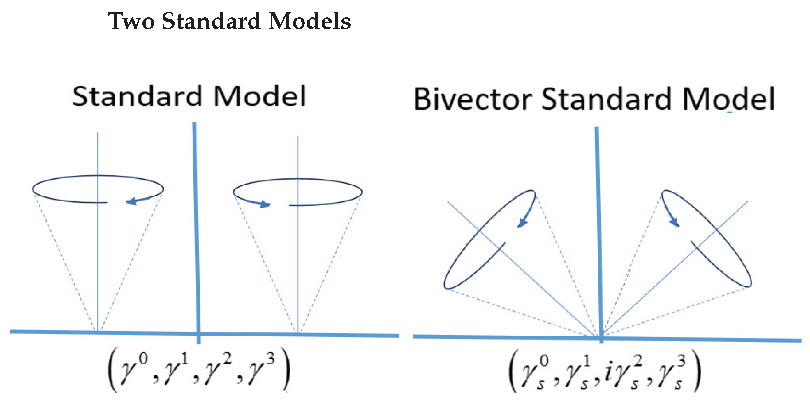
In this work we explore an alternative geometric description in which the electron’s spin is modeled as a bivector, [8,9]. It has two massive, orthogonal axes forming a rigid rotor that precesses about a third axis. This is illustrated in Figure 1, left panel, and arises naturally in a geometric-algebra (GA) formulation, [10], with a different metric signature than the usual SM spinor representation. This motivates a new Bivector SM (BiSM), [9]. Figure 2 contrasts the usual matter–antimatter pair of the SM with the BiSM of two counter-precessing angular-momentum cones on a single particle.
The key claim is structural and classical: the bivector rotor partitions the electron’s energy between external, field-coupled motion in the Laboratory Fixed Frame (LFF), and an internal, mass-like motion in the Body Fixed Frame (BFF). We show that this partition can be expressed,
for a rigid bivector with external vector, and internal bivector inertias and , where the factor 4 reflects the doubled precession frequency of the internal blades, [10]. We then recover the usual relation,
and identify the reduced Compton wavelength, [11], , as the radius of the inertial ring and as the electromagnetic coupling scale of the same geometry. Together these relations interpret as a fixed structural ratio that quantifies how only a small fraction of the electron’s content is directly available for electromagnetic coupling.
1.1. Scope and prior work.
The objective is to establish that the FSC emerges as a structural ratio in the BiSM geometry. Since the FSC is the basis for broader topics, we restrict the discussion to it, and defer application to when the internal dynamics of the bivector are developed, [12]. There we discuss such applications as to the Zitterbewegung, zbw, [13], the double slit analysis, g-factor correction, spectra, and radiative shifts. Here we focus only on the geometric origin of which figures in many applications, and provide one illustrative example.
2. The bivector electron
The two massive, orthogonal axes, 1 and 3, define an internal plane 13 which is orthogonal to the linear–momentum axis 2. This can spin with either helicity, Figure (Figure 1), panel 1, [9]. An external torque about axis 2 transfers angular momentum into the internal BFF, producing a centrifugal force along the 13 bisector. In response, cones of angular momentum form around each axis; they counter-precess at a frequency that is twice that of the external torque about axis 2. This is a geometric realisation of the SU(2) double cover over SO(3).
In GA the classical spin bivector is the wedge of the two angular-momentum vectors associated with the internal axes, [9],
Euler’s equations, [14], for a rigid body in the interaction plane 13 yield,
where is the separation angle between the two vectors. The BFF has its own coordinate frame, , a boost and rotation from Minkowski space of the LFF. Equation (4) is written in the basis,
The two cones are mirror images with equal phase and opposite energy. From these, the scalar and bivector, wedge parts are,
Hence the geometric product is a unit quaternion, a rotor in 3D space, parameterized by ,
As the applied torque about 2 increases, the separation angle decreases and the 1 and 3 cones approach. For an electron, the energy required to reach the limiting configuration is small, so the motion rapidly approaches the boundary where the cones touch at . At this boundary, which is within their common 13 reflection plane, the two angular momenta, an intertwine. The two “hands”, the blades form a double helix of mass with even parity. This defines the quantum domain where classical becomes quantum, Figure 2, panel 3.
Isotropy is the absence of external polarization. In this case the electron’s state is , and exhibits only mass. It is EM-inert. In a polarizing field, the double helix is pulled apart so that one axis, with definite chirality, aligns with the field; charge and helicity also emerge and the aligned blade realizes one of the states both of which are EM-active.
The geometric product, Equation (7), suggests a natural partition: as changes, the scalar mass part and the bivector’s internal rotational part are balanced. This motivates the internal–external split developed in Section (Section 3), where the fixed ratio between the external, field-coupled motion and the total rest energy is related to the FSC.
Equations (3) to (7) give a complete BiSM description of classical spin which has a quantum limit. This replaces the definition of spin from the SM.
2.1. Classical rotor Lagrangian and FSC partition
For completeness, we summarize [9] the ingredients needed to justify the energy split used here. In the classical domain, the bivector rotor is driven by a torque about the LFF, Y or 2-axis. Part of this energy is transferred to the internal counter-precession of the 1 and 3 axes in the BFF. The classical Lagrangian follows from Equation (57) of reference [9], writing,
where we distinguish two sets of indices. The BFF signature has two spatial dimensions of with indices . This convention leads to the mass term being positive, . The LFF indices are denoted by . This allows representing the equations with either BFF indices, or LFF indices, and transform between them. For example,
The matrix changes basis between the BFF frame and the LFF, with
The rotor is precessing at high velocity (rim speed of the cones is ,9]), relative to the LFF and there is no single global Lorentz transform between them. Instead we use an instantaneous transformation and map to the LFF by a local boost at time , , followed by Wigner-Thomas rotation , [22]. For this rim speed, one finds the Lorentz factor of , so the net precession seen in the LFF differs from the non-relativistic value by a few percent. This justifies treating the LFF as an instantaneous boost+rotation of the BFF while including the Thomas correction when needed.
Although not standard in physics notation, we intentionally display mixed BFF and LFF components in Equation (8) to make the frame split transparent. Physically, the internal rotor dynamics reside in the BFF, while the interaction with external fields is expressed in the LFF. Convention uses indices from the LFF, so the bivector rotor current, , couples to an external potential, , and the field-strength bivector tensor is defined by,
Here represents the external electromagnetic potential acting on the rotor, while represents the same expressed in the BFF. is its field tensor; mass, M, follows from the scalar in Equation (7), thereby replacing the Higgs mechanism; and is the rotor current aligned with the torque axis.
In the quantum limit, [9], the same geometry separates these two frames into two complementary domains. This bifurcation distinguishes the symmetry of the LFF (reflection) from that of the BFF (parity). The internal bivector motion in the BFF has definite even parity while the external vector torque axis has definite odd parity. In the quantum domain, matter is separated from force; in the classical domain, they are geometrically mixed between two different frames. The classical domains becomes quantum when .
For the FSC, we need only the kinematic consequence of the internal rotor’s geometry. That is the projection of the internal motion from the BFF to the LFF is visible, and therefore, as a projection, it does not give the full bivector dynamics. Those internal BFF blades, , in the plane, counter-precess at twice the laboratory torque frequency around axis 2: the manifestation of the double cover. We use this to partition the energy and separate the internal inertial energy of the rotor in the BFF from its electromagnetic coupling energy in the LFF. The ratio of these two contributions, set by the geometry and double-cover structure, is what yields the fine-structure constant in the BiSM approach.
3. The Fine-Structure Constant
The empirical FSC is, [15],
This section shows that the same geometry that fixes the inertial and EM rings also fixes the share of energy available to each. No renormalization is required because the BiSM electron has intrinsic physical scales . These provide natural ultraviolet bounds, in contrast to the SM where divergences are removed by renormalization [16,17,18]. Low-energy quantities, including , are obtained here without an ad hoc cutoff.
Write the rotational energies in the usual rigid-body form, , with the effective moment of inertia for the laboratory vector motion and for the internal bivector motion. From Equation (1) this implies that
The inertial ring is identified with reduced Compton length, , which we take as the ring radius. Likewise, the laboratory coupling ring is the classical radius, . The geometric ratio is consistent with its experimental value. We can take a further step because the bivector’s two blades counter-precess such that the internal blades carry twice the precession frequency of the torque axis; this is the origin of the factor of 4,
Assuming a rigid bivector, the ratio of the external energy from its helicity, and the internal energy of the bivector is fixed at the above ratio. From this, we parameterize the FSC by,
Solving for the inertia ratio and using the value of gives,
These two values confirm that most stored rotational energy is internal while only a small external part is field-coupled. The values of and are found using the standard definitions [15,21,22]:
Thus is a structural ratio in the bivector geometry,
In the BiSM, the electron’s self-energy, , is the portion of internal rotational energy that becomes available when the spin changes from the isotropic state to a polarized state. Part of the confined rotational kinetic energy moves into field-coupled external motion on the perimeter. Thus the state is EM-inert, whereas the polarized states, , are EM-active; the required energy is “self” because it originates in the electron’s own structure and dynamics rather than from an external source.
From the LFF, spin is only the projection of the internal 2D rotor at the Compton scale and depends on the rotor’s mass, . The polarized states emerge from the internal static helix to generate the dynamic helicity degree of freedom in the LFF. There it becomes field-coupled, enabling energy exchange at a scale set by .
In summary, the internal transition transfers a fixed share of the electron’s structural energy content between internal confinement to external, field-coupled motion on the perimeter, governed by the quaternion, Equation (7).
sets inertia, sets EM coupling.
3.1. Thomson Scattering
In the Thomson limit, , the Lorentz force exerts only a small classical acceleration, a, on the electron [19]. The radiated power scales as . The incident intensity also scales as ,20]. Hence the scattering cross section, , is independent of the wave amplitude of . Physically, recoil is negligible, the electron behaves as a harmonically driven charge, and the result is fixed by geometry. The total Thomson cross section is [19,20,21,22]
where is the classical electron radius. Equation (19) follows from integrating the classical dipole scattering pattern, over solid angle [22,23]. Using the fine-structure constant and the reduced Compton wavelength , the classical radius can be written in the equivalent forms . Substituting into Equation (19) yields
making it clear that the area scale is the intrinsic Compton length suppressed by the square of the coupling and hence is small. The numerical value in Equation (20) agrees with experiment to better than when evaluated with CODATA constants [23,24].
In the Thomson regime the only available length is , so no additional dimensionless parameter appears and is constant in . When , however, photon–electron energy–momentum exchange is non-negligible: the outgoing photon frequency shifts to the Compton scale, introducing the ratio and leading to the Klein–Nishina cross section. The Thomson result is the limit of Klein–Nishina, as expected from the correspondence principle, [23,25,26].
Within the BiSM, the electron is a confined bivector rotor whose internal energy resides in the BFF, while only a thin electromagnetic perimeter is visible in the LFF. This share of the Compton-scale structure that can couple to external fields is fixed by , so the effective Thomson radius is and the observable area scales as , reproducing Equation (20). Thus the smallness of has a direct physical meaning: external fields probe only an -weighted rim of the bivector rotor; the bulk of the energy remains confined.
The Thomson cross section is reproduced numerically by both the SM and the present BiSM. The distinction lies not in the value, but in the interpretation. The BiSM scale follows directly from the internal bivector geometry and the –weighted energy share. This gives a mechanical origin for a quantity that in conventional QED is inserted phenomenologically. Thomson scattering offers a quantitative and physical success of the BiSM “energy-share’’ principle, and thereby gives deeper insight into Thomson Scattering. The intrinsic Compton length sets the scale, while sets accessibility.
4. Discussion
The FSC quantifies how much of the electron’s energy is externally EM-active versus internally inertial. With , then the EM-active part is set by ,
This is a coupling or activation scale for the rim dynamics implied by the geometry, and not a discrete spectral line. Because the LFF carries odd parity and the BFF carries even parity, transitions between them are parity-forbidden, and thus do not produce radiative lines. The energy corresponds to core-electron excitations in the few-keV regime. This is accessible to electron-induced X-ray experiments reviewed by [27,28]. This energy represents a natural geometric, or coupling, threshold between the inertial and electromagnetic domains carried by the bivector electron.
The internal BFF preserves mass and spin of the electron and does not participate directly in EM coupling. Only a fraction of the electron’s structure is visible to a field, while the bulk provides inertial stability. This view is consistent with the electron’s capacity to transfer energy, momentum, and torque to a receptor [9]. Its electromagnetic component acts as an extended hand at the rim scale , thereby conveying chirality and mediating the coupling, but not using much energy. Most of the mass–energy remains confined in the inertial ring at the Compton scale and available to be transferred to a receptor to build structures, [9]. Hence the smallness of reflects confinement of energy in the internal bivector rather than an unexplained numerical coincidence.
This article follows as an application of the BiSM, [9], and only focuses on establishing the geometric origin of . These properties and other anomalies depend on the internal bivector dynamics, related to the zbw and electron properties of charge and helicity, [9]. Those appear in forthcoming articles, [12], that rely on structural results obtained here.
The SM treats the electron as a point excitation of a chiral spinor field and introduces the fine-structure constant as an empirical coupling parameter. Within QFT, no internal scale or structural mechanism fixes the value of ; its numerical value must be measured and renormalization is required to manage ultraviolet divergences arising from the point-particle idealization. In contrast, the BiSM assigns the electron a definite internal geometry with intrinsic length scales, and the partition of inertial and electromagnetic degrees of freedom yields as a structural ratio. While the SM successfully organizes and predicts a broad phenomenology, its point-like electron offers no geometric interpretation of the fine-structure constant. The present work therefore suggests that may be understood not as a fundamental parameter to be fitted, but as a consequence of a deeper internal structure that classical and quantum descriptions share.
Note added in proof
After preliminary acceptance of this paper, Santos and Fleury [29] reported a toroidal electromagnetic model of the electron, in which circulating fields confined within a torus, reproduce the QED values of charge, spin , and magnetic moment. Their parameters are addusted to satify constraints, with major torus radius and minor radius . Using the BiSM, the same geometry emerges naturally and is not imposed: the torus appears to represent the projection of the bivector rotor into spacetime (1,3). The internal bivector radius , (the classical radius here, defining the electromagnetic coupling), corresponds to the torus minor radius . The external precession radius corresponds to inertia from the torus major radius . The ratio follows structurally from the coupling between confined and propagating energy, not from parameter fitting.
Although the two approaches reach similar geometric conclusions, their ontologies differ, [9]. Santos and Fleury maintain a purely electromagnetic ontology featuring circulating rotating waves confined to a toroidal geometry. This demonstrates compliance with QED phenomenology, though the current formulation incorporates only a single angular dependency, with a two-angle parameterization planned for subsequent papers. The bivector spin already satisfies that by distinguishing the BFF, where the bivector , Equation (3), rotates from the LFF, and the observed spin arises from the projection of that rotor. Hence, in BiSM the bivector is the physical entity, while the torus is its visible projection in real space; the bivector structure imposes the natural quantum limit, whereas the toroidal model fits parameters to match QED values.
For the two approaches to coincide, the torus would need to be reinterpreted not as a physical ring of circulating fields but as the projection of a bivector rotor. Both approaches recognize the need for intrinsic internal motion and thereby obviate the notion of a structureless point particle. While Santos and Fleury describe this motion as a phase circulating in a toroidal field confined to real space, the BiSM interprets it as the physical bivector rotation in the BFF, whose projection appears toroidal in the LFF. In this sense the two approaches converge, each replacing the point electron with a self-contained, dynamic structure.
Funding
This research received no external funding.
Data Availability Statement
No data generated.
Conflicts of Interest
The author declares no conflicts of interest.
References
- Eddington, A. S. , & Whittaker, E. T. (1946). Fundamental theory.
- P. A. M. Dirac,“A New Basis for Cosmology,” Proceedings of the Royal Society A 165, 199–208 (1938).
- R. P. Feynman, QED: The Strange Theory of Light and Matter, Princeton University Press, 1985.
- R. P. Feynman, R. B. Leighton, and M. Sands, The Feynman Lectures on Physics, Vol. 1, Addison-Wesley, 1964.
- L. Morel, Z. Yao, P. Cladé, and S. Guellati Khélifa, “Determination of the fine-structure constant with an atom-interferometric measurement of the recoil velocity of rubidium,” Nature 588, 61–65 (2020). [CrossRef]
- R. H. Parker, C. Yu, W. Zhong, B. Estey, and H. Müller, “Measurement of the fine-structure constant as a test of the Standard Model,” Science 360, 191–195 (2018). [CrossRef]
- P. Cladé and S. Guellatihyp Khélifa, “The fine structure constant α and the ratio h/m,” Comptes Rendus Physique 20(1–2), 77–92 (2019). [CrossRef]
- Sanctuary, B. Quaternion Spin. Mathematics 2024, 12, 1962. [Google Scholar] [CrossRef]
- Sanctuary, B. The Classical Origin of Spin: Vectors Versus Bivectors. Axioms 2025, 14, 668. [Google Scholar] [CrossRef]
- Doran, C. , Lasenby, J., (2003). Geometric algebra for physicists. Cambridge University Press.
- A. H. Compton,“A Quantum Theory of the Scattering of X-rays by Light Elements, ”Phys. Rev. 21, 483–502 (1923).
- Sanctuary, B. Applications of Bivector spin. In preparation.
- Hestenes, D. The zitterbewegung interpretation of quantum mechanics. Found. Phys. 1990, 20, 1213–1232. [Google Scholar] [CrossRef]
- Goldstein, H. (2011). Classical mechanics. Pearson Education India.
- CODATA 2022 Recommended Values of the Fundamental Physical Constants, National Institute of Standards and Technology (NIST) web database. Available online: https://physics.nist.gov/cuu/Constants/.
- Wilson, K. G. (1971). Renormalization group and critical phenomena. I. Renormalization group and the Kadanoff scaling picture. Physical review B, 4(9), 3174.
- Pauli, W. Villars, F. (1949). On the invariant regularization in relativistic quantum theory. Reviews of Modern Physics 21(3), 434. [CrossRef]
- Doplicher, S. Fredenhagen, K., & Roberts, J. E. (1995). The quantum structure of spacetime at the Planck scale and quantum fields. Communications in Mathematical Physics 172(1), 187–220.
- Damm, Hannes, Ekkehard Pasch, Andreas Dinklage, Jürgen Baldzuhn, S. A. Bozhenkov, Kai Jakob Brunner, Florian Effenberg et al. "First results from an event synchronized—high repetition Thomson scattering system at Wendelstein 7-X." Journal of Instrumentation 14, no. 09 (2019): C09037.
- Geltman, S. (2013). Topics in atomic collision theory (Vol. 30). Academic Press.
- Griffiths, David (2009). Introduction to Elementary Particles. pp. 59–60. ISBN 978-3-527-40601-2.
- J. D. Jackson, Classical Electrodynamics, 3rd ed. (Wiley, 1999), Secs. 14–16.
- Rybicki, G. B. , & Lightman, A. P. (2024). Radiative processes in astrophysics. John Wiley & Sons.
- Mohr, P. J. Taylor, B. N. (1999). CODATA recommended values of the fundamental physical constants: 1998. Journal of Physical and Chemical Reference Data 28, 1713–1852. [CrossRef]
- Heitler, W. (1984). The quantum theory of radiation. Courier Corporation.
- Klein, O. , & Nishina, Y. (1929). Über die Streuung von Strahlung durch freie Elektronen nach der neuen relativistischen Quantendynamik von Dirac. Zeitschrift für Physik, 52(11), 853-868.
- Egerton, R.F. Electron Energy-Loss Spectroscopy in the Electron Microscope, 4th ed. (Springer, 2021).
- Rehr, J.J. & Ankudinov, A.L. “Progress in the theory and interpretation of X-ray spectra.” Coord. Chem. Rev. 249, 131–140 (2005).
- Carlos A., M. dos Santos1 & Marc J. J. Fleury Ann. Fond. Louis de Broglie 49, 1–17, 2025.
Figure 1.
Classical spin’s bifurcation from reflection to parity. From Left to Right: 1. Bivector electron as a rotor: body-fixed blades along precess about . The inertial ring has radius ; the EM-coupling rim is characterized by . 2. the details of the double helix with left and right reflection intertwined to give a state of even parity. 3. The two mirror-image precession states, , represent Nature’s left and right hands. The angles between axes 1 and 3 and their angular momentum vectors are equal in both states and increase with precession frequency. A mirror plane bisects the 1–3 axes. As , the double helix forms. This is the quantum state. 4. The cone is decomposed into components and , orthogonal and parallel to the precession axis.
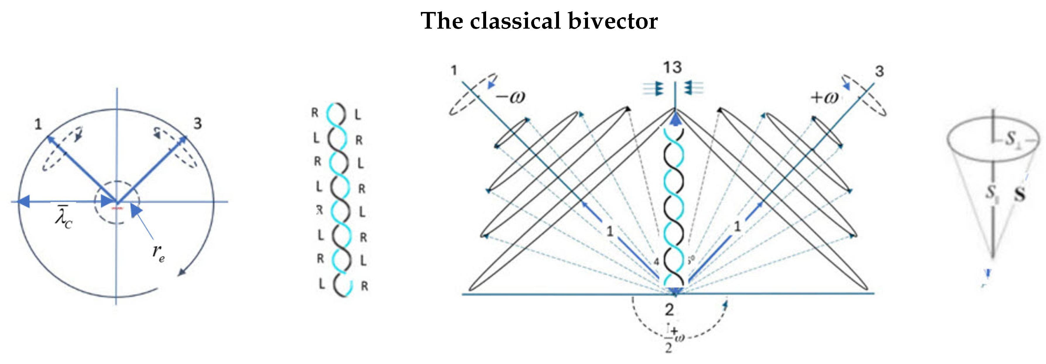
Figure 2.
Left: Dirac’s matter–antimatter pair of the SM. Right: The BiSM showing two counter-precessing angular momentum cones on the same particle that form a bivector.
Figure 2.
Left: Dirac’s matter–antimatter pair of the SM. Right: The BiSM showing two counter-precessing angular momentum cones on the same particle that form a bivector.
Disclaimer/Publisher’s Note: The statements, opinions and data contained in all publications are solely those of the individual author(s) and contributor(s) and not of MDPI and/or the editor(s). MDPI and/or the editor(s) disclaim responsibility for any injury to people or property resulting from any ideas, methods, instructions or products referred to in the content. |
© 2025 by the authors. Licensee MDPI, Basel, Switzerland. This article is an open access article distributed under the terms and conditions of the Creative Commons Attribution (CC BY) license (http://creativecommons.org/licenses/by/4.0/).
Copyright: This open access article is published under a Creative Commons CC BY 4.0 license, which permit the free download, distribution, and reuse, provided that the author and preprint are cited in any reuse.


