
Submitted:
07 November 2025
Posted:
11 November 2025
You are already at the latest version
Abstract
Aiming at the problem of the scale difference between the measurement area model and the real model caused by low-quality images and low-precision control points in the vi-sion three-dimensional deformation monitoring by unmanned aerial vehicles (UAVs), which affects the accuracy of deformation monitoring, the paper develops a spatial 3D scale used to provide high-precision scale information, and puts forward a 3D scale-constrained UAV vision deformation monitoring method, which improves the ac-curacy of deformation monitoring in a wide range of measurement areas. The experi-mental results show that, compared with the monitoring method using only control points as constraints, the method in this paper has an improvement rate of 38.6% and 48.1% in monitoring accuracy in the horizontal and elevation directions in the four-phase UAV operation, which verifies the validity and reliability of the UAV-vision deformation monitoring method with three-dimensional scale constraints.
Keywords:
3D scale
; UAV
; vision measurement
; deformation monitoring
1. Introduction
Vision measurement is a method that uses computer vision technology to analyze and process images and videos in order to obtain information such as the position, shape and size of target objects. It features non-contact, low-cost and high-precision characteristics, and is often used for deformation monitoring of structures like bridges and buildings[1,2].With the rapid development of UAV hardware and software systems, the performance of UAV has greatly improved, and research on methods combining UAV with visual measurement has been continuously advancing in areas such as landslide disaster identification[3] and deep foundation pit deformation[4].Structure from Motion (SfM)[5,6] is a method that detects and tracks feature points from a sequence of multi-view images and reconstructs a 3D model based on the visual motion relationships between the feature points. This method allows rapid acquisition of the 3D model of the object being measured and can be applied to model construction and 3D inspection in scenarios such as slopes, coastal cliffs, and tunnels[7,8,9,10].At present, 3D deformation monitoring using UAVs combined with SfM is mostly used for general survey-type disaster detection or for low-accuracy centimeter- to decimeter-level deformation monitoring[11,12], which cannot meet the requirements for high-precision engineering deformation monitoring applications. Existing studies have indicated that lower image quality[13,14,15] and the limited placement of control points[16,17] are significant factors affecting the accuracy of model reconstruction in survey areas. In UAV-based visual three-dimensional deformation monitoring, the following issues are observed: 1) During UAV operations, complex conditions both on the UAV itself and within the survey area (such as changes in lighting, occlusions, and short exposure times) can lead to low-quality UAV image data, characterized by overexposure, underexposure, blurriness, and shadow occlusion. These conditions affect the extraction of feature information and the detection and positioning of various markers in the survey area, thereby impacting the accuracy of the survey area models and the final deformation monitoring results;2) In deformation monitoring scenarios, there are potential deformation risks inside the survey area, so control points can only be arranged in stable areas at the edge of the survey area. These control points are sparse and unevenly distributed, leading to insufficient control effects on the survey area model and thus affecting the deformation monitoring accuracy. The impact of the above issues on the accuracy of 3D visual deformation monitoring largely manifests as the scale difference between the generated model and the real model. In order to make the constructed model closer to the model with actual physical dimensions, some scholars have used high-precision rulers in the field of industrial photogrammetry to determine the length reference of the measurement coordinate system, thereby improving the measurement accuracy of the system[18].However, in large-scale deformation monitoring scenarios, existing scales cannot be inclined at an appropriate position to enhance scale information in the elevation direction; meanwhile, due to the high flight altitude of drones, existing scales cannot accurately locate both ends in low-quality image data, which tends to dilute the high precision of the scale itself; additionally, a single scale can easily cause random errors, while using multiple scales increases costs.
To address the above problems, this study first designs and develops a spatial 3D scale ruler for providing high-precision scale conversion coefficients, and proposes a UAV vision-based deformation monitoring method with 3D scale constraints, aiming to achieve higher-precision deformation monitoring in large-scale areas. Finally, experiments are conducted to verify the effectiveness and feasibility of the proposed UAV vision-based deformation monitoring method with 3D scale constraints.
2. Materials and Methods
2.1. Development of Three-Dimensional Spatial Ruler
In the field of UAV measurement, control points can provide high-precision position information for model reconstruction and establish the connection between images and real-world coordinates. However, under measurement conditions where the layout of control points is difficult, the accuracy of model reconstruction cannot be guaranteed, failing to meet the requirements of high-precision UAV 3D deformation monitoring. To improve the accuracy of the survey area model, a ruler with a known length can be placed in the survey area to calculate the scale conversion coefficient, thereby making the scale of the survey area model closer to that of the real model. Existing rulers are mostly rod-shaped structures, which cannot be reliably and stably placed in a tilted manner in the survey area, resulting in insufficient constraints in the vertical direction. Moreover, in close-range photogrammetry scenarios with a flight altitude of several tens of meters, the two ends of the ruler lack effective identification features, and the precision of the ruler itself is greatly diluted. Therefore, based on project requirements, this study designs a spatial 3D scale ruler suitable for UAV vision-based deformation monitoring scenarios with a flight altitude of 25 m, considering aspects such as structural relationships, dimensions, and identification effects. The specific design is as follows: To enable the ruler to provide constraint information in multiple directions, three rods with a length of 0.5 m are used to form the main body of the ruler in a pairwise orthogonal manner, and the ruler is designed in a "two lower, one upper" structure—i.e., two rods form a supporting surface, and one rod is placed vertically to provide height information. Meanwhile, a load-bearing platform is built between the two rods of the supporting surface for placing weights to stabilize the ruler; visual positioning markers for identification are fixed at the endpoints of the three rods. In this study, cross-shaped markers with clear centers are adopted, which have good visual effects during image processing and facilitate the accurate positioning of ruler points. Based on the above design, the spatial 3D scale ruler model shown in Figure 1 is obtained. Through the three ruler edges arranged in space in the ruler model, higher-precision scale information in the horizontal and vertical directions is provided, thereby improving the accuracy of model reconstruction and deformation monitoring.
As shown in Figure 1(a), the spatial 3D bracket consists of a 3D bracket main body, marker support brackets for fixing positioning markers, and a load-bearing platform for stabilizing the ruler model. The spatial 3D scale ruler model built with the spatial 3D bracket can realize simultaneous constraints in the horizontal and vertical directions, and one spatial 3D scale ruler model can provide 3 sets of known length constraints, thereby achieving higher scale precision and effectively avoiding accidental errors caused by a single ruler. In the spatial 3D scale ruler, the upper point forms the 1st and 3rd ruler edges with the lower left point and lower right point respectively, and the lower left point and lower right point form the 2nd ruler edge, as shown in Figure 1(c). Assuming that spatial 3D scale rulers are arranged in one measurement, there are ruler edges in total. For the nth spatial 3D scale ruler (,the following relationships exist:
where represents the actual measured length of the ith ruler edge in the nth ruler, represents the length of the ith ruler edge in the nth ruler under the model coordinate system, and represents the conversion coefficient from the model coordinate system to the real-world coordinate system calculated based on the ith ruler edge in the nth ruler. Furthermore, the average scale conversion coefficient of the nth ruler is calculated according to Formula (2).
where represents the weight coefficient of in the calculation of and ,, are all set to . After obtaining the average scale conversion coefficient of each scale, the final scale conversion coefficient is calculated according to Formula (3).
where represents the scale conversion coefficient of the jth ruler, represents the weight coefficient of in the calculation of and its value is . After obtaining the scale conversion coefficient , the world coordinates of point after scale conversion are calculated according to Formula (4).
where is the world coordinate of point without scale correction. Through Formula (4), more accurate coordinates of monitoring points can be obtained, thereby improving the accuracy of deformation monitoring.
2.2. Workflow of the UAV Vision-Based Deformation Monitoring Method with 3D Scale Constraints
The general workflow of UAV vision-based deformation monitoring using the spatial 3D scale ruler is as follows:
(1) Layout of points in the survey area: Arrange the spatial 3D scale rulers in unobstructed areas, plan the UAV operation route, and conduct UAV image acquisition;
(2) Image quality evaluation: Disable low-quality images in subsequent processing and reconstruct a rough model using UAV POS data;
(3) Locate the positions of feature points such as control points and ruler points, construct the spatial 3D scale ruler, calculate the scale conversion coefficient according to Formula (3), and scale the generated model to the real-world coordinate system;
(4) Export the 3D coordinates of monitoring points in the current phase. Repeat steps (1) to (4) to obtain the 3D coordinates of monitoring points in the next phase, and calculate the difference between the coordinates of the two phases to obtain the deformation value of the two phases of monitoring.
Based on the above workflow, the brief steps of the conventional processing method and the 3D scale constraint-based processing method are shown in Figure 2.
3. Experiment Design
This section mainly verifies the performance and feasibility of the UAV vision-based deformation monitoring method with 3D scale constraints. The proposed method is compared with two other deformation monitoring methods—one using only control points and the other using control points plus a single ruler as constraints—to analyze the accuracy and effectiveness of the proposed method. As shown in Figure 3, the experimental site is an area of approximately 10,081.8 square meters located directly south of the stadium in the new campus of Central South University. To simulate a real monitoring scenario, 4 marked control points are arranged at the edge of the survey area, 11 marked monitoring points inside the survey area, 2 3D sliding table deformation simulation points, and 1 spatial 3D scale ruler.
The various equipment used in the experiment is shown in Figure 4. Among them, the UAV used is the DJI Phantom 4 RTK, a small multi-rotor high-precision aerial survey UAV equipped with a centimeter-level navigation and positioning system, a high-performance imaging system, and professional route planning applications. It can carry out monitoring work quickly and flexibly at a relatively low cost; the measurement markers used in the experiment are cross-shaped with a size of 25 cm × 25 cm, which have the advantages of easy layout and easy identification; the spatial 3D scale ruler is fixed in a non-destructible area within the survey area using a weight stabilization device, with a design accuracy of 1 mm; the main body of the 3D sliding table deformation simulation points is a three-axis sliding table device with scales, and a platform for placing markers is designed on the top of the sliding table. By moving the sliding table by a known distance in different monitoring periods as the preset deformation value, this value is used as an indicator for checking accuracy during result analysis, with an accuracy of 1 mm. The control points are measured using a Leica TS09 total station, with an accuracy of 2.2 mm.
The lengths of each ruler edge of the spatial 3D scale ruler used in the experiment are shown in Table 1:
A total of 3 groups of deformation monitoring operations were conducted in this experiment (4 consecutive phases of UAV operations, and each two consecutive phases of UAV operations constitute one group of deformation monitoring operations). For each phase of UAV operation, 2 groups of dynamic displacement checks and 12 groups of static displacement checks were designed. The dynamic displacement checks were performed using 2 3D sliding table deformation simulation points; the static displacement checks included 11 monitoring marker points arranged in the survey area and 1 distance check value composed of two markers (located in the center of the survey area shown in Figure 3, with a known distance between the centers of the two markers and an accuracy of 1 mm). The theoretical deformation displacement of the monitoring marker points is 0. In the experimental result analysis, 14 groups of check indicators were jointly used for accuracy evaluation.
In this experiment, the sparse point cloud reconstruction step was implemented using the low-quality alignment function of Metashape software to simulate the scenario of poor observation conditions in real UAV operations and explore the accuracy improvement performance of the proposed method under low image quality conditions. The information of UAV operations in each phase is shown in Table 2:
4. Results
The collected image data were processed using the control point method and the control point + 3D scale constraint method respectively, and the processing results of the deformation simulation points in this experiment are shown in Table 3:
As shown in Table 3, compared with the control point method, the control point + 3D scale constraint method has smaller measurement errors in both horizontal and vertical directions, which verifies the effectiveness of the spatial 3D scale ruler in improving monitoring accuracy. To explore the accuracy improvement performance of the spatial 3D scale ruler compared with a single ruler, the data were processed using the control point + single ruler constraint method, where the single ruler edge used was the No. 2 ruler edge of the spatial 3D scale ruler. The processing results are shown in Figure 5:
Based on the experimental results shown in Figure 5, the accuracy improvement rate was calculated according to Formula (5):
where represents the accuracy improvement rate; the subscripts and represent the horizontal and vertical directions respectively; represents the deformation monitoring accuracy of the control point constraint method; represents the deformation monitoring accuracy after adding constraint conditions. The calculation results are shown in Table 4:
It can be seen from Table 4 that under the condition of low image quality, both the deformation monitoring methods of control points + single ruler constraint and control points + 3D scale constraint can improve the monitoring accuracy. Due to the certain slope of the survey area ground and the tilted image acquisition of the UAV camera, the method of ground control points + single ruler constraint can improve the monitoring accuracy in both horizontal and vertical directions, but the accuracy is still at a relatively low level; the control points + 3D scale constraint method has a significantly better accuracy improvement rate in both horizontal and vertical directions than the single ruler constraint method, achieving the best accuracy improvement effect among the three methods in both directions, with the vertical accuracy improvement effect reaching 48.1%, which verifies the constraint effect of the spatial 3D scale ruler model in the vertical direction.
In conclusion, the experimental results of this study show that the proposed UAV vision-based deformation monitoring method with control points and 3D scale constraints can effectively improve the deformation monitoring accuracy in both horizontal and vertical directions; compared with the control point method and the control point + single ruler constraint method, the proposed method achieves better accuracy improvement effects in both horizontal and vertical directions, which verifies the practicality and effectiveness of the proposed method in improving monitoring accuracy.
5. Discussion
Aiming at the scale difference between the survey area model and the real-world model, this study designs and develops a spatial 3D scale ruler model for providing high-precision scale information, and forms a set of UAV vision-based deformation monitoring methods with 3D scale constraints. Experimental results show that the proposed method combining control points with 3D scale constraints can effectively improve the accuracy of deformation monitoring; compared with other methods, the proposed method has a higher monitoring accuracy improvement effect. In addition, the spatial 3D scale ruler has the advantages of low production cost, simple on-site layout, and strong applicability, and can meet the requirements of some high-precision engineering deformation monitoring. In the next step, this research will focus on the UAV vision-based deformation monitoring methods for larger survey areas, higher flight altitudes, and lower image quality to further expand the application prospects of UAV 3D vision-based deformation monitoring methods.
Author Contributions
Conceptualization: Jianlin Liu. Methodology: Jianlin Liu, Deyong Pan, Wujiao Dai. Formal Analysis: Jianlin Liu, Deyong Pan. Investigation: Jianlin Liu. Writing—Original Draft Preparation: Jianlin Liu, Deyong Pan. Writing—Review and Editing: Min Zhou, Lei Xing. Supervision: Zhiwu Yu, Jun Wu. All authors have read and agreed to the published ver-sion of the manuscript.
Funding
Science and Technology Research and Development Program Project of China Railway Group Limited(Major Special Project, No. : 2022-Special-09).
Data Availability Statement
The original contributions presented in this study are included in the article material. Further inquiries can be directed to the corresponding author.
Acknowledgments
The authors sincerely acknowledge the research support provided by the National Engineering Research Center of High-speed Railway Construction Technology, China Railway Group Limited.
Conflicts of Interest
The authors declare no conflicts of interest.
Abbreviations
The following abbreviations are used in this manuscript:
| UAV | Unmanned Aerial Vehicle |
| SfM | Structure from Motion |
| 3D | Three-Dimensional |
| GSD | Ground Sampling Distance |
References
- Dandoš, R.; Mozdřeň, K.; Staňková, H. A New Control Mark for Photogrammetry and Its Localization from Single Image Using Computer Vision. Computer Standards & Interfaces 2018, 56, 41–48. [Google Scholar] [CrossRef]
- Taşçi, L. Deformation Monitoring in Steel Arch Bridges through Close-Range Photogrammetry and the Finite Element Method. Experimental techniques 2015, 39, 3–10. [Google Scholar] [CrossRef]
- Xin, W.; Pu, C.; Liu, W.; Liu, K. Landslide Surface Horizontal Displacement Monitoring Based on Image Recognition Technology and Computer Vision. Geomorphology 2023, 431, 108691. [Google Scholar] [CrossRef]
- Guan, L.; Chen, Y.; Liao, R. Accuracy Analysis for 3D Model Measurement Based on Digital Close-Range Photogrammetry Technique for the Deep Foundation Pit Deformation Monitoring. KSCE Journal of Civil Engineering 2023, 27, 577–589. [Google Scholar] [CrossRef]
- Moulon, P.; Monasse, P.; Marlet, R. Global Fusion of Relative Motions for Robust, Accurate and Scalable Structure from Motion. In Proceedings of the Proceedings of the IEEE international conference on computer vision; 2013; pp. 3248–3255.
- Zhu, S.; Zhang, R.; Zhou, L.; Shen, T.; Fang, T.; Tan, P.; Quan, L. Very Large-Scale Global Sfm by Distributed Motion Averaging. In Proceedings of the Proceedings of the IEEE conference on computer vision and pattern recognition; 2018; pp. 4568–4577.
- Parente, L.; Chandler, J.H.; Dixon, N. Optimising the Quality of an SfM-MVS Slope Monitoring System Using Fixed Cameras. The Photogrammetric Record 2019, 34, 408–427. [Google Scholar] [CrossRef]
- Peppa, M.V.; Mills, J.P.; Moore, P.; Miller, P.E.; Chambers, J.E. Automated Co-registration and Calibration in SfM Photogrammetry for Landslide Change Detection. Earth Surface Processes and Landforms 2019, 44, 287–303. [Google Scholar] [CrossRef]
- Esposito, G.; Salvini, R.; Matano, F.; Sacchi, M.; Danzi, M.; Somma, R.; Troise, C. Multitemporal Monitoring of a Coastal Landslide through SfM-derived Point Cloud Comparison. The Photogrammetric Record 2017, 32, 459–479. [Google Scholar] [CrossRef]
- Xue, Y.; Zhang, S.; Zhou, M.; Zhu, H. Novel SfM-DLT Method for Metro Tunnel 3D Reconstruction and Visualization. Underground Space 2021, 6, 134–141. [Google Scholar] [CrossRef]
- Cardenal, J.; Fernández, T.; Pérez-García, J.L.; Gómez-López, J.M. Measurement of Road Surface Deformation Using Images Captured from UAVs. Remote Sensing 2019, 11, 1507. [Google Scholar] [CrossRef]
- Peppa, M.V.; Mills, J.P.; Moore, P.; Miller, P.E.; Chambers, J.E. Accuracy Assessment of a UAV-Based Landslide Monitoring System. The international archives of the photogrammetry, remote sensing and spatial information sciences 2016, 41, 895–902. [Google Scholar] [CrossRef]
- Mosbrucker, A.R.; Major, J.J.; Spicer, K.R.; Pitlick, J. Camera System Considerations for Geomorphic Applications of SfM Photogrammetry. Earth Surface Processes and Landforms 2017, 42, 969–986. [Google Scholar] [CrossRef]
- Dai, W.; Zheng, G.; Antoniazza, G.; Zhao, F.; Chen, K.; Lu, W.; Lane, S.N. Improving UAV-SfM Photogrammetry for Modelling High-relief Terrain: Image Collection Strategies and Ground Control Quantity. Earth Surface Processes and Landforms 2023, 48, 2884–2899. [Google Scholar] [CrossRef]
- O’Connor, J. Impact of Image Quality on SfM Photogrammetry: Colour, Compression and Noise, Kingston University Kingston, UK, 2018.
- Sanz-Ablanedo, E.; Chandler, J.H.; Rodríguez-Pérez, J.R.; Ordóñez, C. Accuracy of Unmanned Aerial Vehicle (UAV) and SfM Photogrammetry Survey as a Function of the Number and Location of Ground Control Points Used. Remote Sensing 2018, 10, 1606. [Google Scholar] [CrossRef]
- Villanueva, J.K.S.; Blanco, A.C. Optimization of Ground Control Point (GCP) Configuration for Unmanned Aerial Vehicle (UAV) Survey Using Structure from Motion (SFM). The international archives of the photogrammetry, remote sensing and spatial information sciences 2019, 42, 167–174. [Google Scholar] [CrossRef]
- Ye, N.; Zhu, H.; Wei, M.; Zhang, L. Accurate and Dense Point Cloud Generation for Industrial Measurement via Target-Free Photogrammetry. Optics and Lasers in Engineering 2021, 140, 106521. [Google Scholar] [CrossRef]
Figure 1.
Spatial 3D Scale Ruler. (a) Spatial 3D Bracket; (b) Spatial 3D Scale Ruler Model; (c) Ruler Edges.
Figure 1.
Spatial 3D Scale Ruler. (a) Spatial 3D Bracket; (b) Spatial 3D Scale Ruler Model; (c) Ruler Edges.
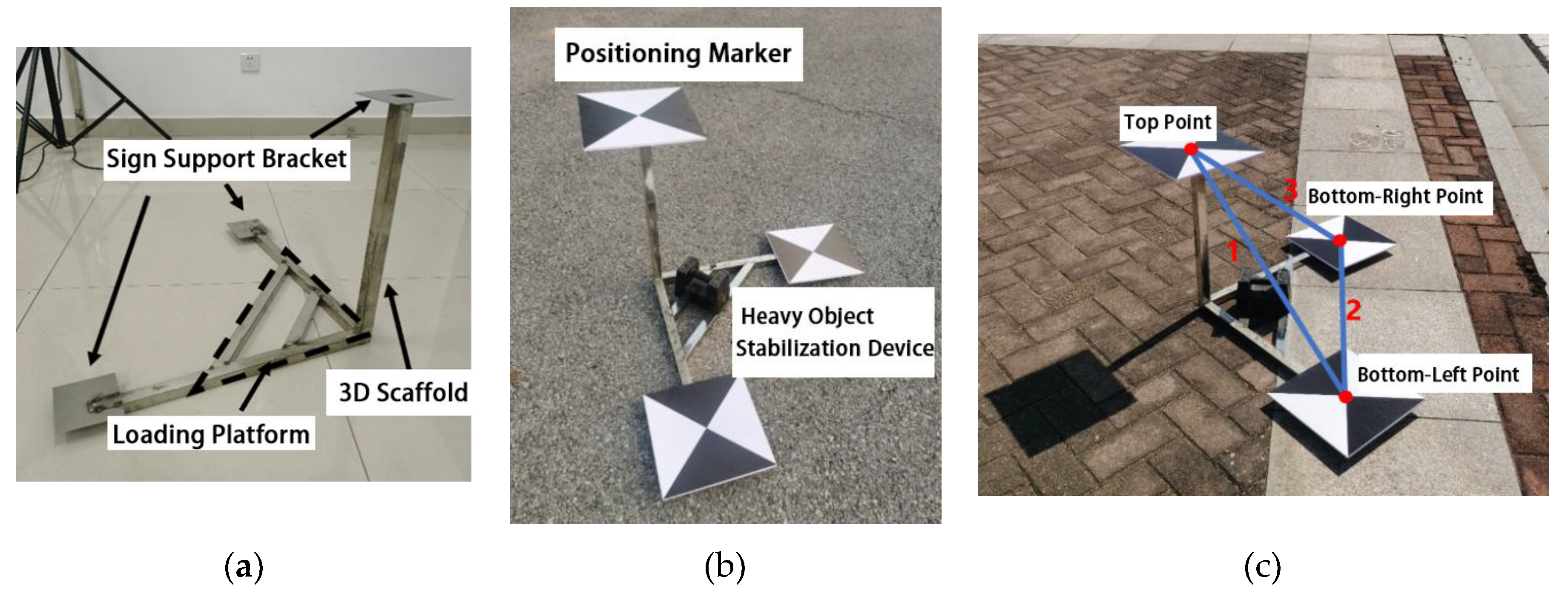
Figure 2.
Figure 2. Workflow of UAV Vision-based Deformation Monitoring with 3D Scale Constraints.
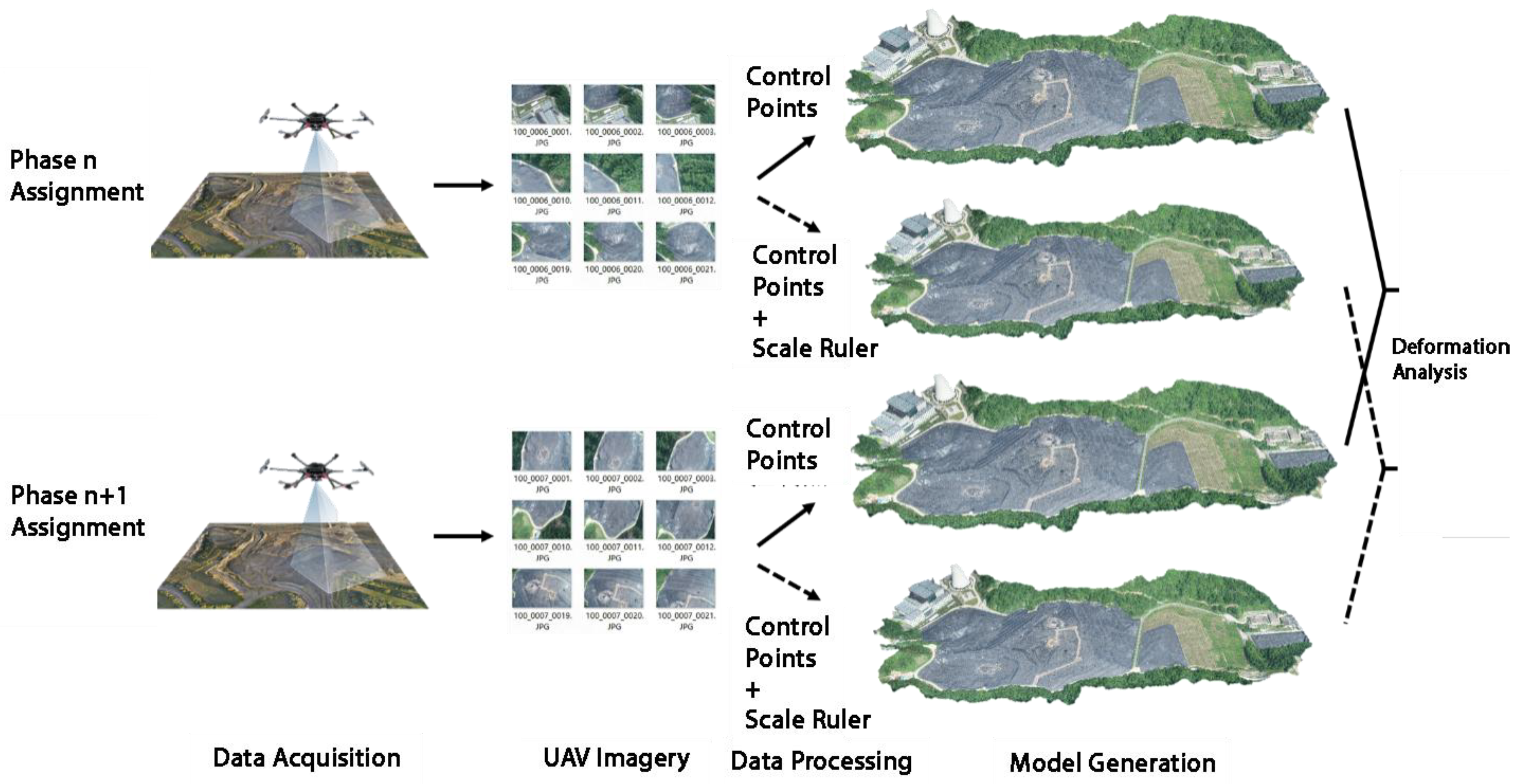
Figure 3.
Schematic Diagram of Experimental Point Layout.
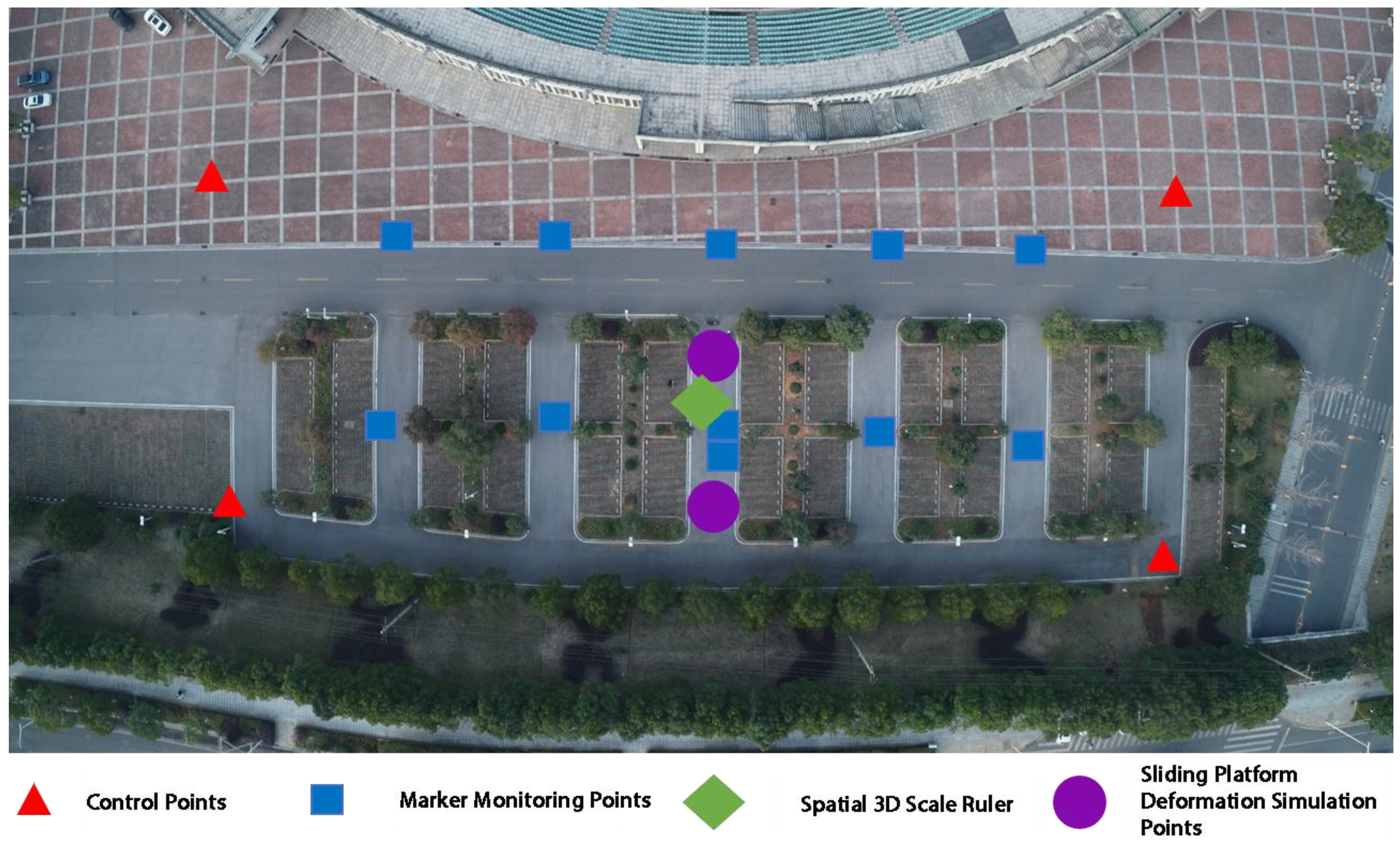
Figure 4.
Figure 4. Experimental Equipment and Materials. (a) Phantom 4 RTK; (b) Markers; (c) Spatial 3D Scale Ruler; (d) 3D Sliding Table.
Figure 4.
Figure 4. Experimental Equipment and Materials. (a) Phantom 4 RTK; (b) Markers; (c) Spatial 3D Scale Ruler; (d) 3D Sliding Table.
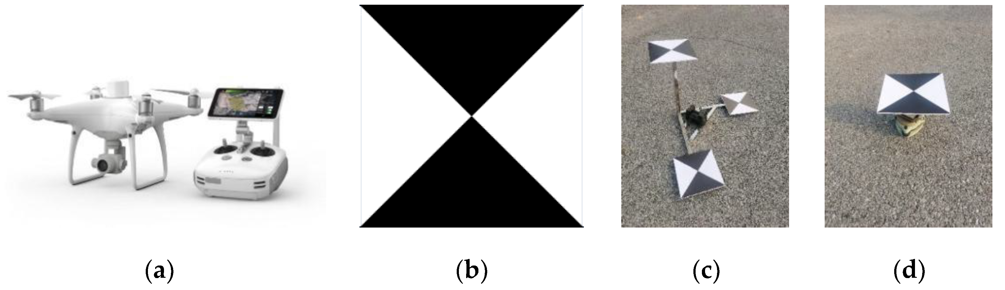
Figure 5.
Experimental Results. (a) Horizontal Monitoring Accuracy of Different Rulers; (b) Vertical Monitoring Accuracy of Different Rulers.
Figure 5.
Experimental Results. (a) Horizontal Monitoring Accuracy of Different Rulers; (b) Vertical Monitoring Accuracy of Different Rulers.
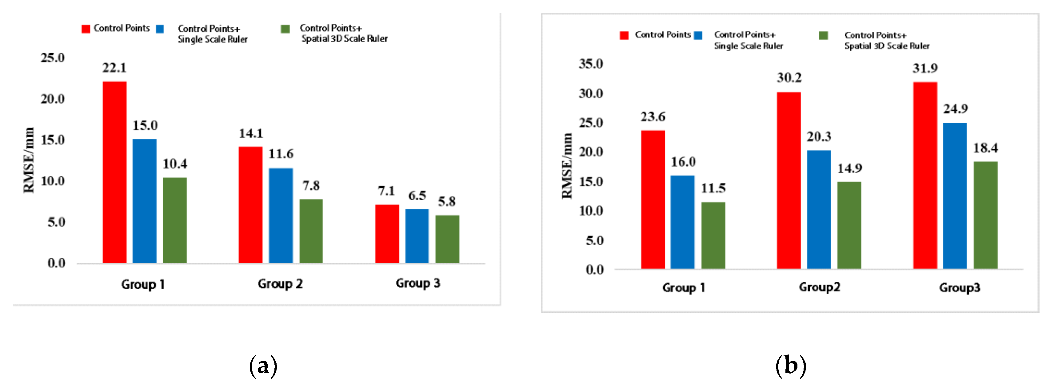

Table 1.
Lengths of Ruler Edges.
| Name of Ruler Edge | Length(m) |
|---|---|
| 1 | 0.7185 |
| 2 | 0.6980 |
| 3 | 0.7194 |
Table 2.
UAV operation information.
| Flight Altitude | Flight Speed | GSD | Overlap Rate (Longitudinal/Lateral) | Camera Model | Camera resolution | Camera focal length | Camera tilt angle |
|---|---|---|---|---|---|---|---|
| 25(m) | 2.4(m/s) | 0.68(cm/pixel) | 80%/75% | FC6310R | 5472*3648 | 8.8(mm) | -60° |
Table 3.
Preset Displacement Values and Measured Values.
| Monitoring Group | Deformation Simulation Point 1 | Deformation Simulation Point 2 | ||||
|---|---|---|---|---|---|---|
| Group 1 | Group 2 | Group 3 | Group 1 | Group 2 | Group 3 | |
| Preset Horizontal Displacement (mm) | 7.1 | 14.1 | 10.0 | 5.0 | 10.0 | 15.0 |
| Horizontal Displacement by Control Point Method (mm) | 15.6 | 12.1 | 6.6 | 37.8 | 29.0 | 12.7 |
| Horizontal Displacement by Proposed Method (mm) | 8.8 | 13.8 | 6.5 | 21.8 | 21.9 | 13.0 |
| Horizontal Absolute Error by Control Point Method (mm) | 8.5 | 2.0 | 3.4 | 32.8 | 19 | 2.3 |
| Horizontal Absolute Error by Proposed Method (mm) | 1.7 | 0.3 | 3.5 | 16.8 | 11.9 | 2.0 |
| Preset Vertical Displacement (mm) | -9.0 | 9.0 | 0.0 | 0.0 | 0.0 | 0.0 |
| Vertical Displacement by Control Point Method (mm) | 8.8 | -12.3 | 30.8 | 42.0 | -51.6 | 32.1 |
| Vertical Displacement by Proposed Method (mm) | -22.4 | 20.5 | 7.8 | 18.0 | -30.7 | 22.6 |
| Vertical Absolute Error by Control Point Method (mm) | 17.8 | 21.3 | 30.8 | 42.0 | 51.6 | 32.1 |
| Vertical Absolute Error by Proposed Method (mm) | 13.4 | 11.5 | 7.8 | 18.0 | 30.7 | 22.6 |
Table 4.
Accuracy Improvement Performance of Various Methods (Compared with the Control Point Method).
Table 4.
Accuracy Improvement Performance of Various Methods (Compared with the Control Point Method).
| Control Points + Single Ruler | Control Points + Spatial 3D Scale Ruler | |||
|---|---|---|---|---|
| Horizontal | Vertical | Horizontal | Vertical | |
| Group 1 | 32.1% | 32.2% | 52.9% | 51.3% |
| Group 2 | 17.7% | 32.8% | 44.7% | 50.7% |
| Group 3 | 8.5% | 21.9% | 18.3% | 42.3% |
| Average | 19.4% | 29.0% | 38.6% | 48.1% |
Disclaimer/Publisher’s Note: The statements, opinions and data contained in all publications are solely those of the individual author(s) and contributor(s) and not of MDPI and/or the editor(s). MDPI and/or the editor(s) disclaim responsibility for any injury to people or property resulting from any ideas, methods, instructions or products referred to in the content. |
© 2025 by the authors. Licensee MDPI, Basel, Switzerland. This article is an open access article distributed under the terms and conditions of the Creative Commons Attribution (CC BY) license (http://creativecommons.org/licenses/by/4.0/).
Copyright: This open access article is published under a Creative Commons CC BY 4.0 license, which permit the free download, distribution, and reuse, provided that the author and preprint are cited in any reuse.


