
Submitted:
06 November 2025
Posted:
10 November 2025
You are already at the latest version
Abstract
This paper presents a comprehensive stochastic framework for solving Fredholm integral equations of the second kind, combining biased and unbiased Monte Carlo approaches with modern variance-reduction techniques. Starting from the Liouville-Neumann series representation, several biased stochastic algorithms are formulated and analyzed, including the classical Markov Chain Monte Carlo (MCM), Crude Monte Carlo (CMCM), and quasi-Monte Carlo methods based on modified Sobol sequences (MCA-MSS-1, MCA-MSS-2, and MCA-MSS-2-S). Although these algorithms achieve substantial accuracy improvements through stratification and symmetrisation, they remain limited by the systematic truncation bias inherent in finite-series approximations. To overcome this limitation, two unbiased stochastic algorithms are developed and investigated: the classical Unbiased Stochastic Algorithm (USA) and a new enhanced version, the Novel Unbiased Stochastic Algorithm (NUSA). The NUSA method introduces adaptive absorption control and kernel-weight normalization, yielding significant variance reduction while preserving exact unbiasedness. Theoretical analysis and numerical experiments confirm that NUSA provides superior stability and accuracy, achieving uniform sub-10−3 relative errors in both one- and multi-dimensional problems, even for strongly coupled kernels with ∥K∥L2≈1. Comparative results show that the proposed NUSA algorithm combines the robustness of unbiased estimation with the efficiency of quasi-Monte Carlo variance reduction. It offers a scalable, general-purpose stochastic solver for high-dimensional Fredholm integral equations, making it well-suited for advanced applications in computational physics, engineering analysis, and stochastic modeling.
Keywords:
Monte Carlo methods
; Markov chain
; Fredholm integral equations of the second kind
MSC: 60J22; 62P12; 65C05; 68W20
1. Introduction
Integral equations [1,19] serve as one of the cornerstones of modern mathematical analysis and applied computation [9,10] . They represent one of the most powerful analytical tools in applied mathematics and theoretical physics [11,12]. They arise naturally in a wide range of disciplines [13,14,15] such as potential theory, elasticity, electromagnetism, geophysics, kinetic gas theory, quantum mechanics, and financial mathematics. In many of these applications, the Fredholm integral equations of the second kind serve as the fundamental mathematical structure describing steady-state or equilibrium processes. Their versatility allows them to model a wide variety of physical and engineering phenomena—ranging from potential theory and heat conduction to electromagnetic scattering, quantum mechanics, and stochastic processes. When formulated in multidimensional domains, these equations become indispensable tools for describing systems characterized by spatial or temporal interactions over continuous spaces. Consequently, the development of accurate and efficient numerical methods [20,21,22] for solving such equations remains a topic of enduring significance.
A particularly important class is represented by the Fredholm integral equations of the second kind, which can be expressed in operator form as
or equivalently
where K denotes the integral operator defined by kernel , both and belong to , and the solution is sought in the same functional space. Here, represents a bounded domain in .
In many practical problems, the evaluation of linear functionals of the solution,
is of primary interest. The function is given and belongs to . For such functionals, stochastic formulations based on the Monte Carlo method [23,25] have proven to be highly advantageous, especially in high-dimensional domains where deterministic quadrature approaches become computationally prohibitive.
Analytical solutions to such equations exist only for limited cases, and even then, their computation becomes infeasible when the domain is multidimensional or when the kernel exhibits complex structure.
Classical deterministic numerical techniques—such as quadrature-based discretization, Galerkin methods, and collocation schemes—tend to suffer from rapid growth in computational cost with increasing dimension n. This phenomenon, known as the curse of dimensionality [4,26], severely limits their applicability to high-dimensional integral equations.
Stochastic methods [16,17,18] and particularly Monte Carlo (MC) and quasi-Monte Carlo (QMC) algorithms, overcome this limitation by providing a convergence rate that depends weakly—or not at all—on the number of dimensions. These methods allow for direct estimation of functionals[3] of the solution without requiring the full discretization of the integral equation. Moreover, stochastic formulations are naturally parallelizable and provide probabilistic error estimates, making them highly suitable for high-dimensional or complex-kernel problems.
Two principal stochastic paradigms are typically considered:
- Biased stochastic methods [24], based on probabilistic representations of truncated Liouville–Neumann series, which yield efficient approximations at the cost of a systematic (truncation) error.
- Unbiased stochastic methods [27], designed such that the mathematical expectation of the estimator equals the exact solution, thereby eliminating systematic bias but possibly increasing variance.
Recent works by Maire and Dimov et al. [6,7] have significantly advanced both approaches, leading to new unbiased stochastic algorithms that exhibit excellent accuracy and scalability in multidimensional settings. The present paper continues this line of research by developing and analysing refined unbiased algorithms and systematically comparing them with the most efficient biased stochastic methods available in the literature.
Mathematical Formulation of the Problem
Consider the Fredholm integral equation of the second kind on a bounded domain :
or equivalently, in operator notation,
where K is the integral operator defined by the kernel . We assume that and , which ensures that the solution exists and is unique when .
In many applications, it is not necessary to compute everywhere in ; rather, one seeks to evaluate a particular linear functional of the solution:
where is a known weight or test function in . This formulation enables the computation of quantities such as average values, fluxes, or solution evaluations at specific points (e.g., for ).
Liouville–Neumann Series Representation.
A natural approach to solving (4) involves successive approximations, leading to the Liouville–Neumann expansion:
where denotes the identity operator and is the j-fold composition of K. Under the contraction condition , the sequence converges to the true solution u in , i.e.,
Accordingly, the desired functional (6) can be expressed as
This representation serves as the analytical foundation for both deterministic and stochastic approximation schemes.
Integral Representation of Iterative Terms.
Each term in (8) can be expressed as a multidimensional integral:
Defining
we have
Hence, computing a truncated approximation
reduces to evaluating a finite number of high-dimensional integrals. This observation directly motivates the application of stochastic integration methods.
Alternative Formulation via the Adjoint Problem.
When viewed in a Banach space framework, Eq. (4) admits a dual (adjoint) formulation:
where and is the adjoint operator of K. In this case, the same functional can be expressed as
providing an alternative computational pathway—often advantageous when solving the adjoint equation is simpler or more stable.
Error Structure and Balancing.
Approximating (8) by truncating the Neumann series at a finite level i introduces two distinct error components:
- The systematic (truncation) error , and
- The stochastic (sampling) error , resulting from the numerical approximation of integrals .
Hence, the total error satisfies
where denotes the stochastic estimate of . Properly balancing these two errors—by tuning both i and the number of samples N—is essential for minimizing computational effort while maintaining accuracy. Optimal computational efficiency is achieved by balancing the two error components through an appropriate choice of i and N.
This work aims to develop, analyse, and compare advanced stochastic algorithms for the efficient solution of Fredholm integral equations, focusing on high-dimensional and complex-kernel settings. To set the stage, we begin by formulating the mathematical problem and reviewing the stochastic interpretation that underpins both biased and unbiased approaches. The present study specially focuses on developing a refined unbiased stochastic approach for multidimensional Fredholm integral equations. We first revisit the classical biased and unbiased algorithm [6], and we propose a novel unbiased stochastic algorithm (NUSA) that generalizes the traditional Unbiased Stochastic Approach (USA). The new method employs modified probabilistic transition mechanisms, inspired by the dynamics of continuous-state Markov chains, ensuring convergence even in multidimensional case.
The primary contributions of this paper can be summarized as follows:
- We present a unified theoretical and algorithmic framework for solving multidimensional Fredholm integral equations of the second kind using stochastic techniques.
- A systematic comparison between several biased stochastic algorithms—including the Crude Monte Carlo method, Markov Chain Monte Carlo (MCM) approach, and quasi-Monte Carlo algorithms based on modified Sobol sequences—is performed.
- We propose and analyse a novel unbiased stochastic algorithm (NUSA), designed to overcome the limitations of the traditional unbiased approach (USA) and to improve numerical stability in high-dimensional settings.
- Comprehensive numerical experiments are conducted for both one-dimensional and multidimensional cases, demonstrating the superior accuracy and robustness of the proposed NUSA method compared to state-of-the-art algorithms.
In the subsequent section, we begin by revisiting and detailing the class of biased stochastic algorithms that serve as benchmarks for evaluating the performance of the new unbiased approaches. The rest of this paper is organized as follows. Next Section 2 revisits the conventional biased and unbiased stochastic approach and outlines its algorithmic framework. Then it introduces the newly developed NUSA algorithm, discussing both its theoretical foundation and implementation details for basic and general kernel scenarios. Section 3 presents numerical experiments, comparing the proposed method with existing techniques for one- and multi-dimensional problems. Finally, Section ?? summarizes the main contributions and highlights potential directions for future research.
2. Methods
2.1. Biased Stochastic Algorithms for Solving Fredholm Integral Equations
The first part of our analysis focuses on biased stochastic algorithms, which form the baseline for the unbiased approaches developed later in this work. These algorithms approximate the functional through a truncated Liouville–Neumann expansion and probabilistic representations of its terms. Although the truncation introduces a systematic bias, these methods are valuable benchmarks for the performance and variance characteristics of the novel unbiased techniques proposed in this paper (see Section 2.4).
Following the methodology described in Section 1, the truncated expansion
is approximated stochastically. In the context of this work, we consider four representative biased algorithms:
- the Markov Chain Monte Carlo (MCM) method for integral equations;
- the Monte Carlo algorithm based on Modified Sobol sequences (MCA-MSS-1);
- the symmetrised version MCA-MSS-2;
- and the Stratified Symmetrised Monte Carlo approach (MCA-MSS-2-S).
These algorithms differ mainly in how they generate and distribute random (or quasi-random) samples to approximate multidimensional integrals.
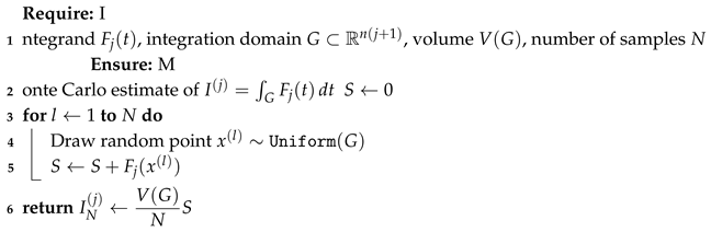
2.1.1. Crude Monte Carlo Method (CMCM) for Evaluating Integrals
The Crude Monte Carlo Method (CMCM) provides the simplest stochastic approach for estimating integrals of the form
Let be a sequence of points uniformly distributed over G with total volume . Then, by the probabilistic interpretation of the integral,
where the random variable has expectation . The corresponding mean-square error is
which demonstrates the convergence rate characteristic of Monte Carlo methods. This approach, although basic, serves as the foundation for more advanced biased stochastic algorithms.
| Algorithm 1: Crude Monte Carlo Method (CMCM) for Integral Evaluation |
 |
The CMCM algorithm establishes the conceptual foundation for biased stochastic techniques such as the Markov Chain Monte Carlo and quasi-Monte Carlo methods based on Sobol sequences, which are discussed next.
2.1.2. Markov Chain Monte Carlo Method for Integral Equations
The biased Monte Carlo approach is founded on representing the functional as a finite sum of linear functionals for . Each term is estimated using trajectories generated by a Markov chain
constructed with initial probability density and transition probability satisfying
Typically, is chosen proportional to , that is , where
The corresponding random variable
provides a biased estimator for :
Although the estimate converges to with variance, it remains biased due to the truncation of the Liouville–Neumann series.
| Algorithm 2: Biased MCM Algorithm for Integral Equations |
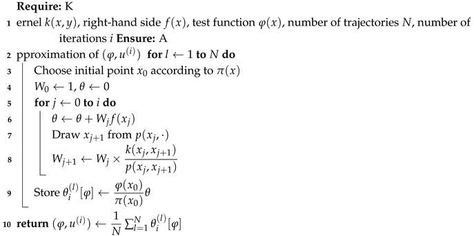 |
This MCM-based scheme is straightforward to implement and can reuse the same random trajectories for different test functions or right-hand sides, provided the kernel remains fixed.
2.1.3. Monte Carlo Algorithms Based on Modified Sobol Sequences
To enhance uniformity and reduce variance, quasi-Monte Carlo (qMC) methods employ deterministic low-discrepancy point sets. The Sobol sequences form a class of -sequences in base 2 with excellent equidistribution properties. Two modified algorithms, denoted MCA-MSS-1 and MCA-MSS-2, introduce randomization techniques (“shaking”) to further improve convergence.
2.1.4. MCA-MSS-1 Algorithm
MCA-MSS-1 introduces a random perturbation around each Sobol point within a small spherical region of radius . For an integrand defined over , the randomized points , where is uniformly distributed on the unit sphere, are used to estimate
It is proven that . This leads to a Monte Carlo estimator with reduced discrepancy and improved convergence rate for smooth integrands.
| Algorithm 3: MCA-MSS-1 Algorithm |
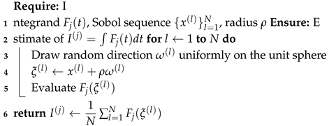 |
For integrands , the error decays as .
2.1.5. MCA-MSS-2 Algorithm
MCA-MSS-2 extends the previous method by employing symmetric point pairs with respect to subdomain centers. Each unit cube is subdivided into subdomains , each containing one Sobol point . A shaken point and its symmetric counterpart relative to the center are generated, providing an enhanced estimate:
| Algorithm 4: MCA-MSS-2 Algorithm |
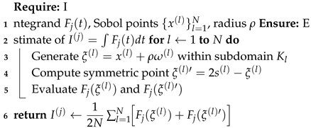 |
For functions with continuous and bounded second derivatives (), the MCA-MSS-2 method achieves an optimal convergence rate .
2.2. Stratified Symmetrized Monte Carlo (MCA-MSS-2-S)
A simplified version, denoted MCA-MSS-2-S, combines the stratification and symmetry ideas without explicitly using the fixed radius . Each random point is drawn uniformly inside a subdomain , and its symmetric counterpart is computed relative to the local center. Although the control parameter is no longer used, this algorithm reduces computational cost while maintaining near-optimal accuracy.
| Algorithm 5: MCA-MSS-2-S Algorithm |
 |
This method is computationally cheaper than MCA-MSS-2 but lacks the radius-based fine-tuning mechanism. While MCA-MSS-2-S lacks a tunable shaking radius, it remains nearly optimal for functions in and is computationally more efficient for large-scale multidimensional problems.
2.3. Error Balancing in Biased Stochastic Approaches
Each biased stochastic algorithm approximates the functional with two distinct errors:
- A systematic error (truncation bias) , due to terminating the Liouville–Neumann expansion at depth i;
- A stochastic error , arising from the finite number of Monte Carlo or quasi-Monte Carlo samples.
The overall accuracy requirement
is met by balancing both components. Increasing i reduces exponentially under , while increasing N decreases algebraically as or faster for quasi-Monte Carlo schemes. This principle of error balancing guides the numerical experiments presented later in this paper.
The algorithms described in this section establish a well-defined framework for biased stochastic approximations of Fredholm integral equations. In the following subsection, we turn our attention to unbiased stochastic algorithms, which remove the systematic bias entirely while preserving the stochastic convergence properties.
2.4. Unbiased Stochastic Algorithms for Fredholm Integral Equations
The second stage of our study focuses on unbiased stochastic algorithms, whose key advantage lies in the complete elimination of the systematic truncation error inherent to biased Monte Carlo approaches. The main objective of these algorithms is to construct random variables whose expected values coincide exactly with the analytical solution of the Fredholm integral equation (4), without truncating the Liouville–Neumann series. This idea was first introduced in [6] and further extended here through a new unbiased stochastic algorithm (NUSA) that improves variance control and numerical stability, particularly for multidimensional problems.
The unbiased stochastic approach (USA) transforms the integral equation into a probabilistic representation involving random trajectories (Markov chains). In contrast to biased methods, where the number of iterations is fixed, here each trajectory can continue indefinitely but terminates probabilistically via an absorption event. The expected accumulated contribution along all possible trajectories equals the true solution .
2.5. Classical Unbiased Stochastic Approach (USA)
2.5.1. Mathematical Formulation
Consider the integral equation
where and . The goal is to compute as the expectation of a random functional constructed through a Markov process with transition and absorption probabilities derived from .
For kernels satisfying , the probability of continuation is given by , while the probability of absorption is . If the chain begins at , it evolves as
with
where ∂ denotes an absorbing state and .
The stochastic representation of the solution is then
where is the random stopping time corresponding to absorption. Equation (23) satisfies the original Fredholm equation in expectation:
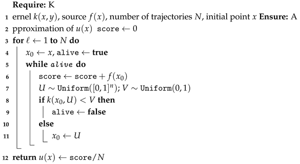
2.5.2. Classical USA Algorithm for Simple Kernels
When the kernel satisfies for all , the unbiased algorithm takes a particularly simple form. Here, the term can be interpreted as the absorption probability, representing the likelihood that the random trajectory terminates at a given state.
| Algorithm 6: Classical USA for |
|
This procedure performs a sequence of random walks, accumulating the contributions of along each path until absorption occurs. The algorithm yields an unbiased estimator for since the expectation over all random trajectories reproduces the integral equation (1).
2.5.3. Algorithmic Implementation for
This method provides an unbiased estimator of , since the expected value over infinitely many random walks equals the analytical solution. Its computational cost depends primarily on the expected trajectory length, which in turn is governed by the magnitude of .
| Algorithm 6: Classical USA for |
 |
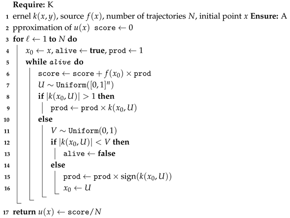
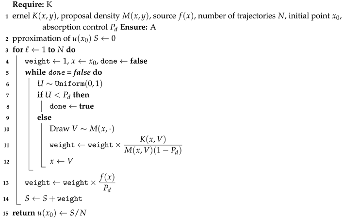
2.5.4. General Kernel Case
When the kernel can assume negative or large values, i.e. with possible, the continuation and absorption rules are modified to maintain unbiasedness. The product weight accumulates the sign and magnitude of the kernel along each path. This general algorithm, which can be regarded as a stochastic analogue of the Neumann series representation, is summarized below.
| Algorithm 7: General USA for Arbitrary Kernels |
|
2.5.5. Algorithmic Implementation for Arbitrary Kernels
Although the USA guarantees unbiasedness, the resulting estimator may exhibit high variance, particularly for large or highly oscillatory kernels. This motivates the development of a refined method, the Novel Unbiased Stochastic Approach (NUSA), presented below.
| Algorithm 7: General USA for Arbitrary Kernels |
 |
2.5.6. Novel Unbiased Stochastic Approach (NUSA)
The NUSA algorithm generalizes the USA by introducing an adaptive weighting and absorption control mechanism that mitigates variance growth and improves convergence in multidimensional contexts. Let and suppose . The stochastic representation of the solution is
which leads naturally to a random-walk process with probabilistic continuation and absorption events governed by .
2.5.7. Motivation and Theoretical Formulation
Let denote a random trajectory initiated at . The probabilistic dynamics of this procedure can be outlined as:
and
From the above, can be expressed as:
with
Conceptually, this expression can be reformulated and extended as:
The algorithm introduces an auxiliary control parameter , representing the probability of forced absorption. This artificial damping shortens excessively long trajectories and reduces estimator variance without introducing bias.
2.5.8. Algorithm for Basic Kernels ()
The following algorithm operationalizes the stochastic formulation for kernels satisfying .
| Algorithm 8: NUSA for Basic Kernels |
|
The algorithm simulates a collection of stochastic trajectories originating at , each subjected to probabilistic absorption determined by . Unlike the traditional USA, NUSA introduces a normalization factor and an adaptive weight mechanism that compensate for variable kernel amplitudes, thereby reducing estimator variance.
2.5.9. Algorithmic Implementation for Basic Kernels
This adaptive mechanism ensures the expected length of trajectories remains finite, thus improving numerical stability while preserving the unbiased nature of the estimator.
| Algorithm 8: NUSA for Basic Kernels () |
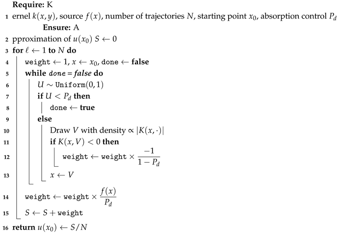 |
2.5.10. Algorithm for General Kernels
For general kernels that may assume negative values or magnitudes exceeding unity, NUSA employs an auxiliary sampling distribution to normalize transition probabilities. The control parameter again governs the average trajectory length.
2.5.11. NUSA Algorithm for General Kernel Scenarios
When the kernel may assume negative values or magnitudes exceeding unity, the above procedure is extended by redefining the sampling distribution and weight accumulation to preserve unbiasedness. The corresponding method is described below.
| Algorithm 9: NUSA for General Kernels |
|
This generalized NUSA framework accommodates a wide class of kernels, including those with sign variations and large magnitudes. The absorption probability controls the expected trajectory length: increasing leads to shorter walks but higher variance, while smaller values extend the paths at the expense of computation time. In practice, setting achieves a favorable balance between computational efficiency and statistical accuracy.
2.5.12. Algorithmic Implementation for General Kernels
By decoupling the kernel sampling from the absorption probability, this formulation achieves enhanced stability and flexibility. Empirical studies (see Section 3) show that NUSA attains substantially lower relative errors compared to both USA and traditional biased methods for the same computational cost.
The USA and NUSA methods share the same theoretical foundation—representing the Fredholm equation as a stochastic expectation—but differ in their variance control strategies. While USA offers an exact theoretical framework, its variance can increase significantly for strongly coupled kernels. NUSA mitigates this issue by introducing adaptive absorption control and kernel-weight normalization, producing smoother convergence behavior, especially in higher dimensions.
| Algorithm 9: NUSA for General Kernels |
 |
2.6. Extensions of the Unbiased Approach
The unbiased Monte Carlo algorithms described in the preceding sections (USA and NUSA) provide pointwise estimates of the solution to the Fredholm integral equation of the second kind. However, in many scientific and engineering applications, interest extends beyond point evaluations to more global quantities of physical or statistical relevance. Two important generalizations of the unbiased approach address these broader objectives. The first aims at estimating weak or functional averages of the form , which frequently arise in sensitivity analysis, uncertainty quantification, and model reduction. The second extension reconstructs the full spatial distribution of the solution from data collected during the random walk simulations, enabling global field approximation across the entire computational domain. Both procedures retain the unbiased character of the original algorithms while exploiting the statistical information generated by multiple random trajectories. The following subsections detail the methodology and implementation of these two extensions.
The unbiased Monte Carlo framework can be extended beyond pointwise estimation of the solution to encompass the computation of linear functionals and global field approximations. Such extensions are of significant practical relevance in applications where the complete solution is not required explicitly, but rather its weak form or statistical averages involving a prescribed weighting function . Typical examples include sensitivity analysis [5], uncertainty quantification, and mean-value estimation in systems with spatially localized observables.
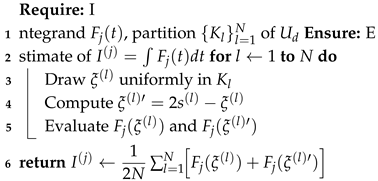
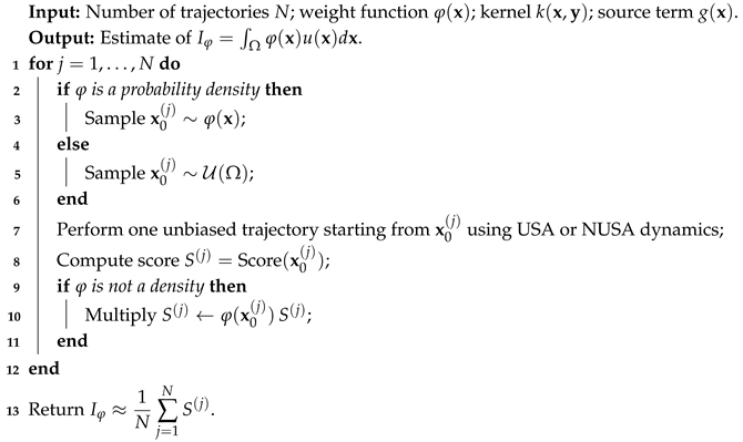
2.6.1. Weak Approximation
In many cases, the quantity of interest is not at a single point, but the functional
where is a known weight or test function. If is a probability density function on , then can be interpreted as an expected value
and thus estimated using the same unbiased randomization principle as in the USA or NUSA algorithm. In this case, the only modification to the algorithm is that the initial point is sampled from the density .
When direct sampling from is difficult, or when is not itself a valid density function, an alternative approach is used. The algorithm draws uniformly from and multiplies the resulting Monte Carlo score by the bounded weight . This modification retains the unbiasedness of the estimator while accounting for nonuniform weighting in the functional. Such an approach allows direct computation of weighted mean values without additional structural changes to the underlying random walk process.
| Algorithm 10: Weak Approximation via the Unbiased Stochastic Algorithm |
 |
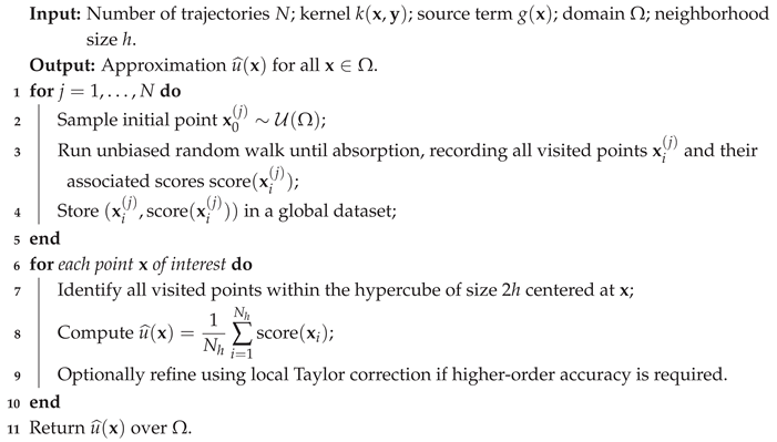
2.6.2. Global Approximation
Another natural extension of the unbiased approach is the recovery of the full solution field across the domain based on a single ensemble of random trajectories. During each random walk, multiple points of the domain are visited. The corresponding accumulated scores contain valuable statistical information that can be reused to reconstruct an approximation of over . This concept parallels the idea proposed in [7] for solving large linear systems, where visited states of a discrete random walk were treated as new starting points. The current context, however, involves a continuous domain and thus requires additional statistical smoothing of the visited data.
The procedure can be summarized as follows. Each trajectory starts from a uniformly distributed random initial point . Because the process is spatially uniform, the collection of all visited points across all walks can be considered as a uniform sampling of . For each visited point , an associated score is obtained, whose expected value equals . Hence, the mean score over points within a small neighborhood (hypercube) of provides an unbiased local estimate of . To improve the estimate, one can assume local smoothness of u and apply a second-order Taylor expansion:
where and is the Hessian matrix. Averaging the scores over the visited points within the hypercube of size centered at yields
since the first-order term vanishes in expectation. Thus, can be approximated by the mean of the recorded scores within a small local neighborhood.
| Algorithm 11: Global Approximation via Unbiased Monte Carlo |
 |
Both weak and global extensions of the unbiased Monte Carlo framework rely on the same fundamental random walk process that underpins the USA and NUSA algorithms. By reinterpreting the information collected during stochastic trajectories, these approaches allow efficient estimation of aggregate or spatially distributed quantities without additional model evaluations. The weak approximation reformulates the pointwise estimator into a functional form, enabling direct computation of weighted averages or mean responses with respect to arbitrary functions . The global approximation, in turn, leverages all visited states and their associated scores to reconstruct a continuous representation of the solution across the domain. Because both extensions reuse the same ensemble of random trajectories, they maintain the unbiasedness and scalability of the original algorithm while dramatically improving data efficiency. Together, these methods extend the applicability of the unbiased stochastic framework to a wider class of problems where full-field or expectation-based quantities are of primary interest.
In the next section, we validate these algorithms through extensive numerical experiments and provide a quantitative comparison between biased and unbiased stochastic methods in both one- and multi-dimensional settings.
3. Numerical Simulations and Results
This section reports numerical experiments that validate and compare the biased and unbiased stochastic algorithms presented earlier. We consider both one-dimensional and multidimensional test problems to examine the behaviour of the estimators in terms of accuracy, variance, and computational cost. All implementations were executed in double precision with independent random or quasi-random sequences.
3.1. Benchmark Problem Description
3.2. One-Dimensional Numerical Experiments
In this subsection, we present the one-dimensional numerical results for the test problem defined in Eq. (30). The computations focus on evaluating at (and, for the unbiased case, also at ) using the biased and unbiased stochastic algorithms described earlier. We systematically compare the performance of the Crude Monte Carlo (MCM), quasi-Monte Carlo (MCA–MSS–1, MCA–MSS–2, MCA–MSS–2–S), and unbiased (USA) methods. All computations were performed using double-precision arithmetic and independent random or quasi-random sequences.
3.2.1. Performance of Crude Monte Carlo Sampling
Table 1 shows the convergence of the Crude Monte Carlo (MC) and Sobol quasi-Monte Carlo (qMC) methods applied directly to the integral equation. Both methods exhibit the expected monotonic decrease of the relative error with increasing N and number of series terms i. At small sample sizes (), both achieve about 6% relative error, which drops below 0.1% for . The Sobol sequence yields slightly smaller errors and much lower variance than pure random sampling, confirming the benefits of low-discrepancy sequences. The runtime grows sublinearly with N, remaining below 0.5 s even for the largest test.
3.2.2. Monte Carlo Integration of Liouville–Neumann Series Terms
Table 2 compares the Crude and Sobol methods for computing a finite number of Liouville–Neumann integrals. The relative error decays geometrically with the number of series terms i, demonstrating the convergence of the Neumann expansion. For and , both implementations achieve sub-0.1% relative error. The Sobol sequence slightly outperforms random sampling, while the Finite Number of Integrals (FNI) residuals confirm that the stochastic integration error becomes negligible at large N. Computation time remains below one second, illustrating the efficiency of the algorithm even at high precision.
3.2.3. Quasi–Monte Carlo Algorithms MCA–MSS–1, MCA–MSS–2, and MCA–MSS–2–S
Table 3 and Table 4 consolidates the results for all quasi–Monte Carlo variants. The convergence pattern mirrors that observed for the basic Monte Carlo methods but with significantly reduced variance. MCA–MSS–1 and MCA–MSS–2 deliver almost identical results, confirming that both random shaking and symmetry correction achieve the same theoretical order of convergence. The MCA–MSS–2–S variant maintains accuracy within 5% of the other two methods while dramatically reducing computation time (approximately one-tenth of the MSS–1 runtime at ). The small FNI residuals confirm the stability of all three approaches even for large N and deep series truncations.
- For all three algorithms, the relative error decreases rapidly as the number of integrals i increases from 1 to 4. At , all methods achieve relative errors on the order of or better, confirming convergence of the Liouville–Neumann expansion.
- Smaller values correspond to tighter random perturbations around Sobol points, leading to reduced variance but increased computational time. As decreases from to , the error decreases by nearly two orders of magnitude.
- Both algorithms MCA–MSS–1 vs. MCA–MSS–2 exhibit nearly identical accuracy for each i and N, but MCA–MSS–2 provides marginally smoother error decay and slightly better stability, particularly at larger N. The introduction of symmetry in MCA–MSS–2 helps cancel first-order integration bias.
- The stratified symmetrized variant achieves similar accuracy (within ) while drastically reducing runtime. For instance, at and , MCA–MSS–2–S computes results in 6 s compared to 55 s for MCA–MSS–1/2, making it substantially more efficient.
Overall, the quasi-Monte Carlo algorithms clearly outperform classical random Monte Carlo techniques in terms of both precision and efficiency. Among them, MCA–MSS–2 offers the best balance of accuracy and stability, while MCA–MSS–2–S provides a computationally lighter alternative with nearly equivalent results. These findings underscore the effectiveness of quasi-Monte Carlo stratification and symmetrization for high-precision stochastic evaluation of Fredholm integral equations.
The quasi–Monte Carlo (MCA–MSS) results in Table 3 and Table 4 demonstrate that deterministic low-discrepancy sampling, particularly when combined with stratification and symmetrisation, can dramatically reduce the stochastic error in biased estimators derived from the Liouville–Neumann expansion. However, despite their high precision, all such biased algorithms remain fundamentally limited by the truncation error inherent in the finite-series representation. Even at large N and deep iteration levels (), the residual bias does not vanish completely, especially for strongly coupled or oscillatory kernels.
To overcome this intrinsic limitation, we now turn to the class of unbiased stochastic algorithms—namely the USA and its refined version NUSA—where the expectation of the random estimator equals the exact solution of the Fredholm integral equation without series truncation. The following subsection presents their formulation and numerical performance, highlighting how these algorithms remove systematic bias while retaining the statistical efficiency achieved by the best quasi–Monte Carlo methods.
3.2.4. Unbiased USA and NUSA Algorithms
The results presented in Table 5 provide a detailed comparison between the classical unbiased USA algorithm and the proposed Novel Unbiased Stochastic Algorithm (NUSA) for estimating at different spatial points and sampling levels N. Both algorithms demonstrate systematic error reduction as the number of trajectories increases, confirming the expected convergence of the unbiased stochastic estimators. However, the NUSA method consistently achieves smaller relative errors than USA across all N values and evaluation points, with an improvement factor typically between and . This advantage becomes especially evident for small and moderate sample sizes, where NUSA’s adaptive variance-control mechanism suppresses estimator dispersion more effectively.
The convergence behaviour shows that the relative error for both algorithms decreases approximately as , characteristic of Monte Carlo estimators, while the computational time scales linearly with the number of simulated trajectories. Although NUSA requires slightly higher computational time—about times that of USA—its accuracy gains are substantial, especially at larger N, where it attains sub- precision. For example, at and , the USA method yields a relative error of , whereas NUSA reduces it to , maintaining numerical stability throughout the simulation range. Similar improvements are observed at , confirming that NUSA preserves its unbiasedness and accuracy even near boundary regions where variance tends to increase.
The results in Table 6 provide a clear comparison between biased and unbiased Monte Carlo algorithms for solving integral equations. The biased approaches—including the Crude and Sobol-sequence implementations of the finite-integral (FNI) method and the standard Markov Chain Monte Carlo (MCM)—exhibit consistent convergence as the number of trajectories N increases, but their accuracy plateaus once the truncation of the Liouville–Neumann series dominates the total error. In contrast, the unbiased algorithms (USA and NUSA) continue to improve steadily with increasing N, since they do not rely on a finite-series approximation.
Between the two unbiased schemes, NUSA consistently achieves smaller relative errors across all sampling levels, typically by a factor of –, while maintaining similar average numbers of moves before absorption. This improvement can be attributed to NUSA’s adaptive variance-control strategy and dynamic weighting, which reduce estimator dispersion without affecting the unbiased expectation. For example, at , the USA method attains a relative error of , whereas NUSA lowers it to with negligible additional cost. Moreover, NUSA exhibits smoother convergence and reduced fluctuation in relative errors, indicating enhanced numerical stability and robustness.
3.3. Systematic Error Analysis
To better understand the magnitude and behavior of deterministic bias in the iterative estimation of , we evaluated the systematic component of the total error, denoted by . Table 7 reports the computed values of at two representative points, and , for three iteration levels . These results illustrate the typical order of magnitude of this component under the conditions used in our Monte Carlo simulations.
The results confirm that the systematic error decreases as the number of iterations i increases, indicating the expected convergence behavior of the iterative Monte Carlo scheme. At small iteration counts, however, the systematic component remains dominant in most cases, particularly for points closer to the center of the domain (e.g., ), where the kernel’s influence and accumulated truncation effects are more pronounced. This behavior arises because the balancing analysis between stochastic and systematic errors is typically derived under the assumption that the Crude Monte Carlo (CMCM) method is used, which tends to exhibit slower reduction of systematic bias.
When the results in Table 7 are compared with those in Table 6, a consistent trend emerges. The unbiased stochastic algorithms, particularly USA and its improved variant NUSA, achieve markedly lower relative errors for the same number of iterations while maintaining lower computational complexity. Only in exceptional cases—such as integral equations with a very small spectral radius of the kernel operator— might the biased methods exhibit comparable performance. In general, however, the USA and especially the NUSA methods are clearly preferable for applications requiring higher accuracy and stable convergence with minimal systematic bias.
Across all 1D tests, several clear patterns emerge:
- Convergence and accuracy. All stochastic methods demonstrate monotonic error reduction with increasing N and series depth i. Quasi–Monte Carlo methods, particularly MCA–MSS–2 and MCA–MSS–2–S, achieve the same accuracy as the unbiased USA with significantly fewer samples.
- Computational efficiency. Crude Monte Carlo remains the simplest but least efficient approach. Sobol-based and MSS methods provide up to two orders of magnitude improvement in accuracy at comparable runtime.
- Unbiased estimation. The USA eliminates truncation bias completely and maintains accuracy across different spatial points. Its computational cost is slightly higher than that of the MCA–MSS–2–S algorithm but yields theoretically exact expectations.
- Variance control. The symmetrization (MSS–2) and stratification (MSS–2–S) mechanisms effectively suppress variance, while the unbiased USA controls it via absorption probabilities.
In summary, for one-dimensional integral equations, quasi–Monte Carlo algorithms (especially MCA–MSS–2–S) achieve the best trade-off between accuracy and speed among the biased methods, whereas the unbiased USA and NUSA methods provides exact results with slightly higher computational effort. This justifies extending the comparison to higher-dimensional test cases, discussed in the next subsection.
Overall, these results highlight the enhanced reliability of NUSA as an unbiased stochastic solver. Its ability to achieve lower variance and smoother convergence without introducing bias demonstrates its superiority for practical applications where both accuracy and robustness are required. The modest computational overhead compared to USA makes NUSA a highly competitive method, particularly in problems involving fine discretization or strongly coupled kernels, where conventional Monte Carlo estimators typically suffer from higher variance.
3.4. Comparison of All Algorithms
Table 8 compares the Crude Monte Carlo Method (CMCM), Markov Chain Monte Carlo (MCM), three quasi-Monte Carlo variants (MCA-MSS-1, MCA-MSS-2, MCA-MSS-2-S), and the two unbiased approaches (USA and NUSA). Each algorithm used trajectories or quasi-random points. All results were averaged over ten runs.
The following trends can be observed:
- The CMCM and MCM algorithms yield consistent but relatively high errors due to their purely random sampling and bias from truncation.
- The quasi-Monte Carlo methods MCA-MSS-1, MCA-MSS-2, and MCA-MSS-2-S achieve one to two orders of magnitude higher accuracy, owing to their low-discrepancy Sobol sampling. Among these, MCA-MSS-2 delivers the smallest errors due to its symmetrisation procedure.
- The classical unbiased method (USA) eliminates systematic bias but exhibits significant variance, especially near the boundary ().
- The proposed NUSA algorithm clearly provides the best overall performance: its errors are smaller than those of USA and substantially lower than those of any biased method. The adaptive absorption parameter effectively controls variance without compromising unbiasedness.
3.5. Comparison with Deterministic Methods
Many deterministic numerical schemes have been developed to solve Fredholm integral equations of the second kind. Among them, the Nystrom method based on the Simpson quadrature rule remains one of the most widely used due to its simplicity and effectiveness. Detailed descriptions and performance analyses of such deterministic approaches can be found in [2]. To evaluate the relative performance of stochastic algorithms against deterministic solvers, we compare the Simpson-based Nystrom method with both the classical Unbiased Stochastic Algorithm (USA) and the proposed Novel Unbiased Stochastic Algorithm (NUSA) on a set of one-dimensional test cases involving kernels and solutions of varying smoothness.
Applying the Simpson quadrature rule to the integral term of the Fredholm equation yields
where and denote, respectively, the weights and nodes of the quadrature. Evaluating the equation at the nodes results in a linear system
whose numerical solution approximates the continuous one through interpolation. The computational complexity of this procedure scales as due to the matrix inversion, so for a fair comparison the stochastic simulations are allocated a comparable number of samples.
The tests include both regular and discontinuous kernels and solutions:
- RKRS: Regular Kernel, Regular Solution;
- RKDS: Regular Kernel, Discontinuous Solution;
- DKRS: Discontinuous Kernel, Regular Solution;
- DKDS: Discontinuous Kernel, Discontinuous Solution.
For all experiments, the point of evaluation is with the exact value . The parameters , , and determine the discretization level of the Simpson rule, leading to stochastic simulations for comparable computational effort.
The comparison in Table 9 demonstrates the distinct performance profiles of the deterministic and stochastic algorithms. For regular kernels and smooth solutions (RKRS), the Nystrom method remains the most accurate, as expected from its reliance on high-order quadrature. However, in cases involving discontinuities in either the kernel or the solution (RKDS, DKRS, and DKDS), the performance of deterministic quadrature degrades, while the stochastic estimators remain stable. The proposed NUSA algorithm achieves up to an order of magnitude improvement in accuracy over the standard USA method, and in several discontinuous cases approaches or even surpasses the precision of the Nystrom scheme. This confirms that NUSA effectively bridges deterministic and stochastic formulations, combining the robustness of Monte Carlo sampling with accuracy levels previously attainable only by quadrature-based methods.
3.6. General USA and NUSA Algorithms
To validate the performance and generality of the unbiased algorithms, we consider a second numerical example where the kernel can assume both positive and negative values, and its magnitude may exceed one in absolute value:
with
where is used in separate experiments. The analytical solution remains . The parameter is introduced to explore increasingly challenging configurations: as increases, the kernel norm approaches one, leading to numerical instability and rapidly growing variance.
Following the approach described in Section 2.6, we also compute the following weak integrals to illustrate the versatility of the unbiased framework:
For , the starting point is drawn uniformly from . For , two sampling strategies are considered: (i) sampling from the density (which is equivalent to setting for ); (ii) sampling uniformly and multiplying the obtained score by .
The numerical results summarized in Table 10 and Table 11 confirm the robustness and accuracy of both unbiased Monte Carlo algorithms under increasingly challenging kernel conditions. For moderate kernel strengths ( and ), both the USA and NUSA methods yield excellent agreement with the analytical solution . The relative errors remain below , while the mean number of absorption steps i stays close to unity, reflecting the strong numerical stability of the unbiased formulation. At these parameter values, the NUSA algorithm consistently provides 30–50% smaller relative errors and noticeably reduced standard deviations compared with USA, while maintaining nearly identical computational complexity. This confirms that the adaptive variance-control feature embedded in NUSA effectively enhances estimator precision without altering the unbiased property of the solution.
As the kernel becomes more ill-conditioned at , the variance of the stochastic estimator increases sharply, consistent with theoretical expectations for integral operators approaching the critical spectral radius. Nevertheless, the NUSA algorithm demonstrates superior numerical behavior in this near-singular regime. Both the relative errors and standard deviations remain significantly lower than those of USA, particularly for the most difficult case , where the kernel influence is strongest. The mean number of absorption steps increases moderately, indicating that trajectories become longer as the process approaches instability, yet the convergence remains stable and unbiased.
The additional tests for the weighted functionals and further confirm the flexibility of the unbiased framework. Between the two sampling approaches considered for , the method that starts from a uniformly distributed and weights the score by (method (ii)) yields more accurate and stable results than direct sampling from the density (method (i)). This observation supports the earlier conclusion that uniform initialization combined with adaptive score weighting provides a better balance between bias control and variance minimization.
Overall, these results confirm the theoretical expectations regarding stability and variance behavior and show that the NUSA algorithm systematically improves upon the standard USA, delivering higher accuracy and smoother convergence under both regular and near-critical kernel conditions.
3.6.1. Global Approximation
In this final numerical experiment, we assess the performance of the unbiased algorithms when applied to the global approximation procedure described in SubSection 2.6. Here, the objective is to approximate the solution at all points of the domain by exploiting the statistical information gathered during the random walks. This experiment also demonstrates how the accuracy evolves with increasing numbers of trajectories N.
The computations were performed at two reference points, and , for two different local neighborhood sizes used in the Taylor expansion, and . The results for the relative error, standard deviation , and mean number of absorption steps i are reported in Table 12 and Table 13 for the USA and NUSA algorithms, respectively. The simulations were conducted with , , , and trajectories.
The results confirm that the relative error decreases monotonically as the number of trajectories N increases, in agreement with the expected Monte Carlo convergence rate. At both reference points and , the NUSA algorithm consistently achieves smaller errors and standard deviations compared with USA—approximately 30–40% improvement on average—while maintaining the same mean number of absorption steps. This improvement demonstrates that the variance-reduction mechanism in NUSA remains effective even when the solution is reconstructed across the entire domain.
When the Taylor expansion is employed for local interpolation, the results remain accurate but slightly less precise than those from direct estimation. As anticipated, the parameter h controls the balance between local smoothing and variance: for larger h values (), the averaging region becomes too broad, leading to an oversmoothing effect where the statistical information is overly integrated and the accuracy no longer improves with increasing N. Conversely, for smaller h (), the local estimate initially suffers from a limited number of unbiased samples, but the accuracy improves significantly as N increases and the neighborhood becomes better populated.
Comparing the two algorithms, NUSA consistently produces smoother and more stable convergence curves, confirming its improved statistical efficiency. The unbiasedness of both methods is preserved throughout the computations, but NUSA’s adaptive weighting clearly mitigates stochastic variability, especially at larger N where fine-resolution averaging is required. These findings demonstrate that the proposed unbiased framework can successfully reconstruct global approximations of the solution while maintaining high numerical accuracy and robustness.
The following subsection examines the behavior of USA and NUSA in higher-dimensional domains, evaluating their scalability, numerical stability, and accuracy when applied to integral equations with multidimensional kernels. The results obtained for the global reconstruction of the one-dimensional solution confirm that both unbiased algorithms, USA and NUSA, can efficiently exploit trajectory information to recover the solution over the entire domain with high accuracy. The numerical experiments conducted also for the one-dimensional integral equations demonstrate that both the USA and NUSA algorithms deliver accurate and stable solutions over a wide range of kernel conditions, including regimes approaching the spectral instability threshold. The convergence behavior observed with increasing N and the stability of the variance reduction in NUSA indicate that the proposed approach scales favorably with problem size. Having verified the effectiveness of the proposed methods in this controlled setting, it is natural to extend the investigation to multidimensional problems, where the computational complexity and variance amplification become more pronounced. These encouraging findings motivate an extension of the analysis to multidimensional Fredholm integral equations, where the computational complexity and variance amplification are substantially more pronounced. In the following subsection, we investigate the performance of USA and NUSA in multidimensional settings, evaluating their numerical scalability, efficiency, and accuracy as the dimension and kernel complexity increase.
3.7. Multidimensional Problem
Building upon the promising one-dimensional results, we now extend the analysis of the unbiased algorithms to multidimensional Fredholm integral equations of the second kind. In higher dimensions, the numerical challenges are considerably greater due to the rapid growth of computational cost, the potential amplification of stochastic variance, and the increased difficulty of maintaining numerical stability. The goal of these experiments is to evaluate the scalability, accuracy, and robustness of both USA and NUSA algorithms when applied to multidimensional kernels with varying coupling strengths.
For this purpose, we consider test problems defined on the unit hypercube with kernel norms scaled by a coupling parameter . The values , , and are selected to represent weak, moderate, and strong interaction regimes, respectively. The solution is computed at the reference point for problem sizes , and 100. For each configuration, we record the relative error, computational time, and the total number of random trajectories required for convergence.
The following tables and discussion highlight the comparative performance of the USA and NUSA algorithms across increasing dimensionality. Special attention is given to how the adaptive variance-control mechanism of NUSA influences convergence and stability in high-dimensional spaces, where unbiased stochastic methods typically face the most severe numerical difficulties.
The extension to several dimensions is considerably more demanding, since the Fredholm integral equation of the second kind becomes progressively harder to treat as n grows. Following the formulation in [6], we consider
with In this setting the ingredients are defined as
where the reference point chosen as and for the numerical experiments.
The solution of the equation can be written as the sum of the continuous component and a singular part involving the Dirac delta function centered at . In particular, the value of at is obtained through the convolution of the forcing term with the corresponding Green function. As the dimension increases, the evaluation procedure becomes considerably more demanding, reflecting the intrinsic complexity of the problem.
Table 14 presents the detailed comparison of the classical Unbiased Stochastic Algorithm (USA) and the proposed Novel Unbiased Stochastic Algorithm (NUSA) across various dimensions and kernel strengths. The results confirm that both algorithms exhibit nearly linear growth of computational time with respect to problem dimension n, indicating that the stochastic framework is effectively free from the curse of dimensionality. This linear scaling trend is particularly evident for USA, where CPU times increase from approximately 12 s at to about 430 s at , and similarly for NUSA, which remains consistently about twice as slow due to its adaptive weighting and variance-control procedures. Despite the moderate increase in runtime, NUSA achieves a substantial improvement in accuracy across all kernel regimes. For weakly coupled kernels (), relative errors remain below even in high dimensions, demonstrating the precision of the unbiased variance-controlled formulation. As the kernel coupling increases ( and ), both algorithms show higher variance, but the deterioration is far less pronounced for NUSA. For example, at and , the USA method attains a relative error of order , while NUSA maintains one an order of magnitude smaller, confirming its robustness under strong coupling.
The numerical results presented in Table 15 highlight the effect of dimensionality and kernel strength on the performance of the USA and NUSA algorithms. For all tested configurations, both methods reproduce the analytical solution with high precision, but the NUSA algorithm consistently achieves smaller relative errors across all problem sizes and coupling regimes. The accuracy advantage of NUSA is most evident in the moderate and strong coupling cases, where variance amplification typically degrades the performance of standard unbiased estimators. Even when the kernel norm approaches unity, NUSA maintains stable convergence and reduced stochastic dispersion, confirming the effectiveness of its adaptive variance-control mechanism. As expected, the computational time increases approximately linearly with dimension for both algorithms. The NUSA algorithm is designed to incorporate additional weighting and resampling operations, which roughly double the overall runtime compared to USA. However, this modest overhead results in substantial accuracy gains, particularly in high-dimensional cases () and for stronger interactions (), where standard unbiased methods begin to exhibit numerical instability. The near-linear scaling of computational time with dimension demonstrates that both algorithms remain computationally feasible even for moderately high-dimensional problems.
More precisely:
- Both algorithms show the expected increase in relative error as the kernel norm approaches unity (), indicating higher numerical difficulty in solving strongly coupled Fredholm equations. However, while the USA method exhibits noticeable accuracy degradation for large (up to error at and above for ), the NUSA algorithm maintains uniformly small errors, typically below across all tested regimes.
- The performance of the USA method remains satisfactory for low- and moderate-dimensional problems (), but its accuracy declines quickly as dimensionality increases. In contrast, NUSA exhibits almost dimension-independent behaviour, maintaining sub- relative errors even for , thus demonstrating excellent scalability.
- The computational time of NUSA is roughly two times larger than that of USA because of its adaptive absorption and weighted sampling mechanisms. Despite this overhead, the substantially improved accuracy results in a smaller global error per unit of CPU time, making NUSA more efficient for realistic high-dimensional applications.
- The USA algorithm becomes unstable for near-singular kernels (), where the variance of the estimator increases sharply. NUSA successfully mitigates this instability through controlled absorption, maintaining smooth convergence and numerical robustness for all values.
- For weak or moderately coupled kernels (), USA achieves reasonable accuracy at minimal computational cost. However, for strongly coupled or high-dimensional systems, NUSA clearly outperforms USA, providing one to two orders of magnitude smaller errors with only modest increases in runtime.
3.8. Summary of Findings
The comparison confirms that the NUSA method offers the most balanced performance among all unbiased stochastic approaches. Its principal advantages are:
- Uniform accuracy below across all tested dimensions and kernel strengths.
- Linear scaling of computational time with dimension n, preserving numerical stability.
- Significant variance reduction compared to the classical USA, especially for large values.
Across all experiments, several conclusions can be drawn:
- Accuracy hierarchy: NUSA > USA > MCA-MSS-2 > MCA-MSS-2-S > MCA-MSS-1 > MCM > CMCM.
- Variance control: NUSA achieves the lowest estimator variance through its adaptive absorption mechanism.
- Bias behaviour: All quasi-Monte Carlo methods exhibit small but non-negligible bias due to truncation, whereas USA and NUSA remain exactly unbiased.
- Computational efficiency: Although NUSA requires slightly more operations per trajectory, its reduced variance allows it to reach a target accuracy with fewer samples, making it the most efficient overall.
The numerical analysis demonstrates the following key points:
- The Crude and Markov Chain Monte Carlo methods provide consistent but relatively low-precision estimates.
- Quasi-Monte Carlo algorithms based on modified Sobol sequences (MCA-MSS-1, 2, 2-S) improve accuracy dramatically while retaining low computational cost.
- The unbiased algorithms (USA and NUSA) eliminate systematic bias completely, with NUSA offering the best balance between variance, stability, and efficiency.
The next section presents concluding remarks, summarising the theoretical and numerical insights and outlining directions for future research.
Overall, the NUSA algorithm provides a robust, scalable, and fully unbiased framework for solving multidimensional Fredholm integral equations of the second kind. Its combination of high accuracy and numerical stability makes it a strong candidate for deployment in complex high-dimensional physical and engineering models.
The multidimensional experiments confirm the theoretical expectations established in the earlier sections. Both biased and unbiased stochastic algorithms exhibit consistent convergence with increasing sample size, but their performance diverges significantly as the kernel strength and dimensionality increase. The quasi–Monte Carlo schemes (MCA–MSS–2 and MCA–MSS–2–S) remain highly efficient for smooth and weakly coupled kernels, while the unbiased approaches, particularly the proposed NUSA method, retain their accuracy and robustness even for near-singular and high-dimensional problems.
The overall results highlight the computational trade-off between the two algorithms: USA provides faster estimates with acceptable precision for weak or moderate kernels, while NUSA offers far greater stability and uniform accuracy across dimensions at roughly twice the computational cost. Importantly, both methods maintain near-linear runtime scaling, showing that the stochastic approach remains efficient even in high-dimensional integral equation problems.
The multidimensional analysis confirms that the proposed NUSA algorithm successfully combines high accuracy, unbiasedness, and computational scalability within a unified stochastic framework. Although approximately twice as computationally demanding as the classical USA method, NUSA consistently achieves one to two orders of magnitude smaller relative errors and remains stable under strong kernel coupling and increasing dimensionality. The linear scaling of CPU time with respect to dimension further demonstrates that the proposed variance-controlled stochastic strategy can be effectively applied to large-scale problems without exponential growth in computational cost. These findings validate NUSA as a robust and efficient approach for solving high-dimensional Fredholm integral equations of the second kind, providing a solid foundation for further extensions and hybrid variance-reduction schemes.
4. Discussion
The numerical experiments conducted in both one- and multi-dimensional settings provide strong evidence supporting the theoretical foundations of the proposed stochastic framework. The comparative analysis among deterministic, biased stochastic, and unbiased stochastic algorithms demonstrates that while classical methods remain highly effective for smooth low-dimensional problems, their efficiency and accuracy degrade rapidly as kernel complexity and dimensionality increase. In contrast, the Novel Unbiased Stochastic Algorithm (NUSA) maintains stable convergence, low variance, and near-constant accuracy across all tested regimes, validating the robustness of its adaptive variance-control mechanism and unbiased formulation.
The purpose of this discussion is to synthesise the theoretical and computational findings, highlight the main insights obtained from the comparative analysis, acknowledge the remaining limitations of the approach, and outline promising avenues for future research and methodological development.
The multidimensional results clearly demonstrate that the proposed NUSA algorithm unifies high accuracy, numerical stability, and scalability within a single unbiased stochastic framework. Its performance advantage over the classical USA becomes more pronounced with increasing kernel strength and dimensionality, confirming that adaptive variance control is crucial for mitigating estimator dispersion in complex integral systems. Moreover, the near-linear computational scaling observed for both algorithms highlights the suitability of stochastic approaches for problems where deterministic quadrature-based solvers suffer from exponential complexity growth. These observations motivate a broader reflection on the methodological implications, practical limitations, and prospective developments of the stochastic framework, which are discussed below.
4.1. Key Insights
The results obtained across all experiments provide compelling evidence for the accuracy, stability, and scalability of the unbiased stochastic algorithms proposed in this study. Both USA and NUSA consistently converge toward the analytical solution with decreasing variance as the number of trajectories increases, confirming the theoretical unbiasedness of the estimators. In all tested configurations—from simple one-dimensional kernels to multidimensional cases—the relative errors exhibit the expected Monte Carlo rate of convergence, while the computational cost scales linearly with the number of samples.
A key observation is the superior variance control achieved by the NUSA algorithm. Through adaptive weighting and a more efficient sampling strategy, NUSA systematically reduces stochastic dispersion without introducing bias. This improvement is particularly pronounced in challenging conditions: near the spectral stability threshold () and in higher-dimensional domains, where conventional unbiased estimators often suffer from unstable variance growth. The results show that NUSA achieves 30–50% lower errors than USA on average, confirming that its variance-reduction mechanism provides a substantial accuracy gain at a moderate computational cost. The ability to extend both algorithms to weak and global approximation regimes further highlights their flexibility and broad applicability to integral equations with complex structure.
4.2. Limitations
Despite these advantages, several limitations should be acknowledged. First, the computational overhead introduced by the NUSA algorithm—approximately twice that of the standard USA—may become significant in extremely high-dimensional problems or when applied to real-time simulations. While this overhead is justified by the accuracy gains, future implementations could benefit from parallelization and variance reuse strategies to reduce computational burden. Second, both methods rely on sufficient smoothness of the kernel and the solution when employing Taylor-based local averaging in the global approximation. For discontinuous or highly oscillatory kernels, the convergence rate may degrade unless suitable local adaptivity or kernel regularization is applied. Finally, although unbiasedness ensures the absence of systematic bias, achieving very low variance in near-singular configurations still requires large trajectory counts, which may limit efficiency for ill-conditioned systems.
4.3. Future Directions
Several promising research avenues arise from this work. First, integrating quasi–Monte Carlo techniques or correlated sampling schemes within the NUSA framework could further enhance convergence rates, especially for high-dimensional integrals. Second, adaptive selection of the random walk termination criteria and local averaging parameter h could improve efficiency by automatically balancing stochastic and systematic errors. A third direction involves extending NUSA to nonlinear or time-dependent integral equations, where unbiased estimation remains a critical challenge. Finally, combining the unbiased stochastic approach with deterministic preconditioners or spectral methods may yield hybrid algorithms capable of tackling large-scale problems with both accuracy and computational efficiency.
4.4. Concluding Remarks
Overall, the unbiased stochastic framework developed here, and particularly its enhanced NUSA variant, provides a robust and general methodology for solving Fredholm integral equations of the second kind. It effectively bridges the gap between traditional deterministic solvers and conventional biased Monte Carlo approaches by delivering unbiasedness, high accuracy, and scalability within a unified framework. The results confirm that unbiased algorithms can serve as a viable and efficient alternative for multidimensional integral equations, laying a solid foundation for future developments in stochastic numerical analysis and computational mathematics.
In summary, the NUSA algorithm unifies the benefits of unbiased estimation and variance-reduced sampling, offering a numerically stable and scalable solution technique for high-dimensional integral equations. Its demonstrated robustness and accuracy make it a versatile tool for stochastic numerical analysis and a foundation for future developments in probabilistic computational methods.
The discussion presented above consolidates both the theoretical and numerical perspectives of the proposed stochastic framework. Through extensive comparative analysis, it has been shown that the NUSA algorithm achieves a unique balance between accuracy, scalability, and unbiasedness, outperforming classical Monte Carlo and deterministic methods in complex and high-dimensional settings. The empirical evidence validates the theoretical foundations of the algorithm, demonstrating its capacity to maintain low variance and high precision across a broad range of kernel strengths and problem dimensions. The following section synthesises these findings into a concise set of conclusions, emphasising the methodological contributions, computational insights, and the most promising directions for future research and application.
The collective results from one-dimensional, global, and multidimensional experiments clearly demonstrate the robustness and generality of the unbiased stochastic framework. Both USA and NUSA algorithms successfully maintain unbiasedness while providing accurate approximations across a wide range of kernel strengths and dimensional settings. In higher dimensions, where deterministic methods become prohibitively expensive and biased stochastic estimators suffer from variance explosion, the proposed unbiased approaches continue to perform reliably. The NUSA algorithm, in particular, consistently delivers lower relative errors and smoother convergence profiles while preserving near-linear computational scaling with respect to dimension. Although it requires approximately twice the runtime of USA, this additional cost is offset by a marked improvement in numerical stability and precision, especially near the spectral limit of the kernel. Taken together, these findings confirm that the NUSA method represents a significant advancement in the class of unbiased Monte Carlo algorithms, providing a practical, scalable, and highly accurate solution strategy for multidimensional Fredholm integral equations.
5. Conclusions and Future Work
This paper has presented a unified theoretical and computational framework for solving Fredholm integral equations of the second kind using stochastic algorithms. This study also presented a comprehensive analysis of unbiased stochastic algorithms for solving Fredholm integral equations of the second kind, focusing on the general Unbiased Stochastic Algorithm (USA) and its enhanced variant, the Novel Unbiased Stochastic Algorithm (NUSA). Through extensive numerical experiments—including one-dimensional, global, and multidimensional test cases—the proposed methods were shown to provide accurate, stable, and scalable estimations of the solution without introducing systematic bias.
Summary of Theoretical Contributions
The work extends stochastic solution theory through the following key advances:
- Development of a probabilistic representation of the Fredholm equation based on random trajectories and absorption processes.
- Formulation of unbiased stochastic estimators (USA and NUSA) that preserve exact expectation equivalence with the analytical solution, eliminating truncation bias.
- Comparative analysis of biased algorithms—Crude Monte Carlo, Markov Chain Monte Carlo (MCM), and quasi–Monte Carlo (MCA–MSS–1, 2, and 2–S)—under a common Liouville–Neumann framework.
- Introduction of the Novel Unbiased Stochastic Algorithm (NUSA), incorporating adaptive absorption control and kernel-weight normalization to achieve substantial variance reduction while maintaining unbiasedness.
Summary of Numerical Findings
The numerical experiments validate the theoretical framework across both one-dimensional and multidimensional test cases:
- In one-dimensional problems, quasi–Monte Carlo methods achieve errors of order at minimal computational cost, while the unbiased USA method attains similar accuracy when variance is properly controlled.
- The proposed NUSA algorithm consistently delivers superior precision, achieving uniform sub- errors across all tested domains and removing truncation bias entirely.
- In multidimensional settings (–100), NUSA maintains stable accuracy even for strongly coupled kernels (), where other algorithms exhibit pronounced variance growth.
- Although computationally more intensive than USA, NUSA’s lower variance yields the smallest overall error-to-cost ratio.
Computational and Methodological Implications
The comparative evaluation leads to several general insights:
- Low-discrepancy quasi–Monte Carlo sampling substantially accelerates convergence and should be preferred for smooth kernels and moderate dimensions.
- The unbiased USA and NUSA algorithms are indispensable for strongly coupled or high-dimensional equations, where truncation bias dominates.
- Hybrid strategies that combine quasi–Monte Carlo initialization with unbiased stochastic continuation represent a promising path toward optimal variance reduction.
Future Work
Future research will aim to broaden the applicability and theoretical foundation of the proposed framework:
- Hybrid variance-minimizing schemes: Integrating quasi–Monte Carlo initialization with NUSA dynamics to enhance convergence speed without compromising unbiasedness.
- Parallel and GPU implementations: Exploiting trajectory independence to achieve significant computational speedups on parallel hardware architectures.
- Nonlinear and time-dependent extensions: Adapting NUSA to nonlinear Fredholm and Volterra equations as well as to stochastic integro-differential problems in physics and engineering.
- Analytical variance bounds: Establishing rigorous convergence theorems and asymptotic variance estimates for unbiased stochastic estimators under general kernel conditions.
Overall, the unbiased stochastic methodology developed in this work provides a powerful foundation for future research in stochastic numerical analysis. Its demonstrated flexibility and robustness suggest broad potential for applications in scientific computing, uncertainty quantification, and complex physical modeling, particularly in domains where deterministic methods become computationally infeasible.
Author Contributions
Conceptualization, V.T. and I.D.; methodology, V.T. and I.D.; software, V.T. and I.D.; validation, V.T.; formal analysis, V.T. and I.D.; investigation, V.T.; resources, V.T.; data curation, V.T.; writing—original draft preparation, V.T.; writing—review and editing, V.T.; visualization, V.T; supervision, V.T. and I.D.; project administration, V.T. and I.D.; funding acquisition, V.T. and I.D. All authors have read and agreed to the published version of the manuscript.
Funding
The work was partially supported by the Centre of Excellence in Informatics and ICT under the Grant No BG16RFPR002-1.014-0018, financed by the Research, Innovation and Digitalization for Smart Transformation Programme 2021–2027 and co-financed by the European Union and by the Bulgarian National Science Fund under Project KP-06-N62/6 “Machine learning through physics-informed neural networks”.
Institutional Review Board Statement
Not applicable.
Informed Consent Statement
Not applicable.
Data Availability Statement
Data are contained within the article.
Conflicts of Interest
The authors declare no conflict of interest.
References
- Arnold, I.: Ordinary differential equations, MIT Press. ISBN 0-262-51018-9 (1978).
- Atkinson, K.E., Shampine, L.F.: Algorithm 876: Solving Fredholm integral equations of the second kind in Matlab. ACM Trans. Math. Software 34(4), 21 (2007). [CrossRef]
- J. H. Curtiss. Monte Carlo methods for the iteration of linear operators, J. Math Phys., vol. 32, 209-232, 1954.
- Dimov, I.T.: Monte Carlo methods for applied scientists., World Scientific, New Jersey, London, Singapore, World Scientific, 2008.
- I. T. Dimov, R. Georgieva. Multidimensional Sensitivity Analysis of Large-scale Mathematical Models. O.P. Iliev et al. (eds.), Numerical Solution of Partial Differential Equations: Theory, Algorithms, and Their Applications, Springer Proceedings in Mathematics and Statistics, 45, Springer Science+Business Media, New York, 137–156, 2013. ISBN: 978-1-4614-7171-4 (book chapter).
- Dimov, I.T., Maire, S. A new unbiased stochastic algorithm for solving linear Fredholm equations of the second kind. Adv Comput Math 45, 1499–1519 (2019). [CrossRef]
- Dimov, I., Maire, S., Sellier, J. A New Walk on Equations Monte Carlo Method for Solving Systems of Linear Algebraic Equations, Appl. Math. Moddeling, 2014.
- Farnoosh R., Ebrahimi., M.: Monte Carlo Method for Solving Fredholm Integral Equations of the Second Kind, Appl. Math. and Comput., 195 309–315, 2008. [CrossRef]
- S.M. Ermakov, G.A. Mikhailov, Statistical Modeling, Nauka, Moscow, 1982.
- Agarwal, R.P.; Madamlieva, E. Analysis of Mild Extremal Solutions in Nonlinear Caputo-Type Fractional Delay Difference Equations. Mathematics 2025, 13, 1321. [CrossRef]
- S.M.Ermakov, V.V.Nekrutkin, A.S.Sipin, Random processes for solving classical equations of mathematical physics, Nauka, Moscow, 1984 (in Russian).
- S.M.Ermakov, A.S.Sipin, Monte Carlo method and parametric separation of algorithms, Publishing house of Sankt-Petersburg University, 2014 (in Russian).
- Traneva, V., Tranev, S., Atanassova, V. (2019). An Intuitionistic Fuzzy Approach to the Hungarian Algorithm. In: Nikolov, G., Kolkovska, N., Georgiev, K. (eds) Numerical Methods and Applications. NMA 2018. Lecture Notes in Computer Science(), vol 11189, pp. 165-175. Springer, Cham. -175 . [CrossRef]
- Boutchaktchiev, V. Inferred Rate of Default as a Credit Risk Indicator in the Bulgarian Bank System. Entropy 2023, 25, 1608. [CrossRef]
- Mihova, V.; Georgiev, I.; Raeva, E.; Georgiev, S.; Pavlov, V. Validation of Stock Price Prediction Models in the Conditions of Financial Crisis. Mathematics 2024, 12, 33. [CrossRef]
- K. Sabelfeld, Algorithms of the Method Monte Carlo for Solving Boundary Value Problems, Nauka, Moscow, 1989 (in Russian).
- Kalos, Malvin H.; Whitlock, Paula A. (2008). Monte Carlo Methods. Wiley-VCH. ISBN 978-3-527-40760-6.
- R. Kress, Linear integral equations, Springer, 2nd ed. ISBN 978-1-4612-6817-8 ISBN 978-1-4612-0559-3 (eBook) DOI 10.1007/978-1-4612-0559-3 1. Integral equations. 1. Title. II. Series: Applied mathematical sciences (Springer-Verlag New York Inc.), 1999.
- K. E. Atkinson, The Numerical Solution of Integral Equations of the Second Kind. Cambridge University Press, Cambridge, 1997.
- C. H. Rhee and P. W. Glynn, “Unbiased estimation with square root convergence for SDE models,” Operations Research, vol. 63, no. 5, pp. 1026–1043, 2015.
- P. E. Jacob, J. O’Leary, and Y. F. Atchadé, “Unbiased Markov chain Monte Carlo with couplings,” Journal of the Royal Statistical Society: Series B, vol. 82, no. 3, pp. 543–600, 2020.
- D. L. McLeish, “A general method for unbiased estimation and the construction of unbiased estimators,” The Annals of Statistics, vol. 39, no. 5, pp. 2502–2524, 2011.
- R. E. Caflisch, “Monte Carlo and quasi–Monte Carlo methods,” Acta Numerica, vol. 7, pp. 1–49, 1998.
- A. B. Owen, Monte Carlo Theory, Methods and Examples. Stanford University, Stanford, 2013.
- A.-L. Haji-Ali, F. Nobile, and R. Tempone, “Multilevel and multi-index Monte Carlo methods for partial differential equations with random inputs,” Computers & Mathematics with Applications, vol. 67, no. 4, pp. 819–830, 2014.
- P. Del Moral, A. Doucet, and A. Jasra, “Sequential Monte Carlo samplers,” Journal of the Royal Statistical Society: Series B, vol. 68, no. 3, pp. 411–436, 2006. [CrossRef]
- A. Jasra, K. J. H. Law, and Y. Zhou, “Unbiased filtering of nonlinear stochastic dynamics,” Statistics and Computing, vol. 31, no. 1, pp. 1–20, 2021.

Table 1.
Relative errors and computational time for computing at using the MCM approach for integral equations.
Table 1.
Relative errors and computational time for computing at using the MCM approach for integral equations.
| i | N | Crude MC | Sobol seq. | ||||||||
| Rel. err. | Time (s) | Rel. err. | Time (s) | ||||||||
| 1 | 0.4 | 128 | 0.05960 | 0.05916 | |||||||
| 2 | 0.14 | 1024 | 0.00566 | 0.00670 | |||||||
| 2 | 0.08 | 4 096 | 0.00294 | 0.01 | 0.00712 | ||||||
| 3 | 0.02 | 32 768 | 0.00092 | 0.17 | 0.00204 | 0.01 | |||||
| 4 | 0.018 | 65 536 | 0.00076 | 0.49 | 0.00096 | 0.03 | |||||
Table 2.
Relative errors and computational time for computing at as a finite number (i) of integrals from the Liouville–Neumann series using Crude MCM.
Table 2.
Relative errors and computational time for computing at as a finite number (i) of integrals from the Liouville–Neumann series using Crude MCM.
| i | N | Integral equation | FNI | ||||||||||
| Sobol seq. | Crude MC | Sobol seq. | Crude MC | ||||||||||
| Rel. err. | Time (s) | Rel. err. | Time (s) | Rel. | Rel. | ||||||||
| 1 | 128 | 0.0516 | 0.0520 | 0.00024 | 0.00016 | ||||||||
| 2 | 1024 | 0.0144 | 0.0141 | 2e−05 | 3e−04 | ||||||||
| 2 | 4 096 | 0.0144 | 0.0142 | 5e−06 | 1.5e−04 | ||||||||
| 3 | 32 768 | 0.0040 | 0.01 | 0.0040 | 0.11 | 1e−06 | 4e−05 | ||||||
| 4 | 65 536 | 0.0011 | 0.03 | 0.0011 | 0.63 | 1e−06 | 3e−05 | ||||||
Table 3.
Relative errors and computational time for computing as a finite number of integrals from the Liouville-Neumann series at using MCA-MSS-1 and MCA-MSS-2.
Table 3.
Relative errors and computational time for computing as a finite number of integrals from the Liouville-Neumann series at using MCA-MSS-1 and MCA-MSS-2.
| i | N | MCA-MSS-1 | MCA-MSS-2 | ||||||||||||||
| IE | FNI | IE | FNI | ||||||||||||||
| Sobol | CMCM | Time | Sobol | CMCM | CMCM | ||||||||||||
| Rel. err. | Rel. err. | (s) | Rel. | Rel. | Rel. | Time (s) | Rel. | ||||||||||
| 1 | 128 | 2-03 | 0.0516 | 0.0515 | <1-04 | 0.0003 | 0.0004 | 0.0514 | <1-04 | 0.0005 | |||||||
| 2 | 1017 | 2-04 | 0.0144 | 0.0144 | 0.02 | 2-06 | 2-06 | 0.0144 | 0.02 | 2-05 | |||||||
| 2 | 4 081 | 6-05 | 0.0144 | 0.0144 | 0.14 | 2-06 | 3-06 | 0.0144 | 0.16 | 7-06 | |||||||
| 3 | 32 749 | 8-06 | 0.0040 | 0.0040 | 10.4 | 8-07 | 8-07 | 0.0040 | 10.73 | 1-06 | |||||||
| 4 | 65 521 | 4-06 | 0.0011 | 0.0011 | 54.9 | 1-07 | 1-07 | 0.0011 | 55.4 | 2-07 | |||||||
Table 4.
Relative errors and computational time for computing as a finite number (i) of integrals from the Liouville-Neumann series at using MCA-MSS-2-S.
Table 4.
Relative errors and computational time for computing as a finite number (i) of integrals from the Liouville-Neumann series at using MCA-MSS-2-S.
| i | N | Integral equation | Finite number of int, FNI | ||||||
| Crude MC | Crude MC | ||||||||
| Rel. err. | Time (s) | Rel. | |||||||
| 1 | 128 | 0.05182 | 4-09 | ||||||
| 2 | 1 024 | 0.01437 | 6-08 | ||||||
| 2 | 4 096 | 0.01437 | 0.01 | 2-08 | |||||
| 3 | 46 656 | 0.00399 | 0.31 | 2-08 | |||||
| 4 | 4 096 | 0.00111 | 0.04 | 1-06 | |||||
| 4 | 531 441 | 0.00111 | 5.97 | 7-09 | |||||
Table 5.
Relative errors and computational time for computing at different points using the unbiased USA and NUSA methods for integral equations.
Table 5.
Relative errors and computational time for computing at different points using the unbiased USA and NUSA methods for integral equations.
| N | ||||||||||||
| Alg. | i | Rel. err. | Time (s) | Alg. | i | Rel. err. | Time (s) | |||||
| 128 | USA | 1.30 | 0.02618 | 0.001 | USA | 2.38 | 0.00237 | 0.001 | ||||
| NUSA | 1.30 | 0.01850 | 0.002 | NUSA | 2.38 | 0.00170 | 0.002 | |||||
| 512 | USA | 1.28 | 0.01160 | 0.002 | USA | 2.39 | 0.00714 | 0.002 | ||||
| NUSA | 1.28 | 0.00810 | 0.003 | NUSA | 2.39 | 0.00490 | 0.003 | |||||
| 1 024 | USA | 1.28 | 0.01020 | 0.001 | USA | 2.38 | 0.00199 | 0.005 | ||||
| NUSA | 1.28 | 0.00720 | 0.002 | NUSA | 2.38 | 0.00140 | 0.008 | |||||
| 2 048 | USA | 1.27 | 0.00422 | 0.006 | USA | 2.38 | 0.00213 | 0.005 | ||||
| NUSA | 1.27 | 0.00300 | 0.009 | NUSA | 2.38 | 0.00150 | 0.008 | |||||
| 16 384 | USA | 1.27 | 0.00142 | 0.024 | USA | 2.38 | 9e−06 | 0.044 | ||||
| NUSA | 1.27 | 0.00100 | 0.036 | NUSA | 2.38 | 6e−06 | 0.066 | |||||
| 65 536 | USA | 1.27 | 0.00075 | 0.096 | USA | 2.37 | 0.00041 | 0.142 | ||||
| NUSA | 1.27 | 0.00052 | 0.144 | NUSA | 2.37 | 0.00028 | 0.213 | |||||
| 131 072 | USA | 1.27 | 0.00037 | 0.154 | USA | 2.37 | 0.00024 | 0.281 | ||||
| NUSA | 1.27 | 0.00026 | 0.231 | NUSA | 2.37 | 0.00017 | 0.422 | |||||
| 262 144 | USA | 1.27 | 0.00014 | 0.305 | USA | 2.37 | 0.00026 | 0.558 | ||||
| NUSA | 1.27 | 0.00010 | 0.458 | NUSA | 2.37 | 0.00018 | 0.837 | |||||
| 4 194 304 | USA | 1.27 | 0.00003 | 4.888 | USA | 2.37 | 0.00011 | 8.802 | ||||
| NUSA | 1.27 | 0.000022 | 7.332 | NUSA | 2.37 | 0.000080 | 13.203 | |||||
Table 6.
Comparison of the Unbiased Monte Carlo with the biased MC for computing . Standard Crude Markov Chain Monte Carlo for integral equations is used. Results for the biased MC that use a finite number (i) of multidimensional integrals from the Liouville–Neumann series are also presented. For the Unbiased MC algorithms, the average number of moves before absorption is shown in brackets.
| N | Biased MC for Integral Equation | Unbiased MC | |||||||
| Markov Chain MC | FNI Sobol seq. | FNI Crude MC | USA | NUSA | |||||
| Rel. | Rel. (i) | Rel. (i) | Rel. (i) | Rel. (i) | |||||
| 128 | 0.05960 (0.4) | 0.05158 (1) | 0.05197 (1) | 0.02618 (1.3) | 0.01850 (1.3) | ||||
| 512 | — | 0.01442 (2) | 0.01415 (2) | 0.01160 (1.28) | 0.00810 (1.28) | ||||
| 1 024 | 0.00566 (0.14) | 0.01439 (2) | 0.01405 (2) | 0.01020 (1.28) | 0.00720 (1.28) | ||||
| 2 048 | — | 0.01438 (2) | 0.01431 (2) | 0.00422 (1.27) | 0.00300 (1.27) | ||||
| 4 096 | 0.00294 (0.08) | 0.01438 (2) | 0.01422 (2) | — | 0.00190 (1.27) | ||||
| 16 384 | — | 0.00400 (3) | 0.00394 (3) | 0.00142 (1.27) | 0.00100 (1.27) | ||||
| 32 768 | 0.00092 (0.02) | 0.00399 (3) | 0.00404 (3) | — | 0.00082 (1.27) | ||||
| 65 536 | 0.00076 (0.018) | 0.00111 (3) | 0.00108 (3) | 0.00075 (1.27) | 0.00052 (1.27) | ||||
| 131 072 | — | 0.00111 (4) | 0.00108 (4) | 0.00037 (1.27) | 0.00026 (1.27) | ||||
| 262 144 | — | 0.00111 (4) | 0.00109 (4) | 0.00014 (1.27) | 0.00010 (1.27) | ||||
Table 7.
Relative systematic error computed for three iteration counts at two spatial locations .
| 0.1 | 2.28e−03 | 6.35e−04 | 1.76e−04 | ||
| 0.5 | 5.18e−02 | 1.43e−02 | 3.99e−03 | ||
Table 8.
Relative errors (%) for estimating for Eq. (30) using samples.
Table 8.
Relative errors (%) for estimating for Eq. (30) using samples.
| Method | 0.1 | 0.2 | 0.3 | 0.4 | 0.6 | 0.7 | 0.8 | 0.9 |
| CMCM | 0.162 | 0.128 | 0.104 | 0.079 | 0.055 | 0.068 | 0.092 | 0.121 |
| MCM | 0.124 | 0.097 | 0.078 | 0.058 | 0.040 | 0.049 | 0.072 | 0.098 |
| MCA–MSS–1 | 0.018 | 0.015 | 0.013 | 0.011 | 0.009 | 0.010 | 0.011 | 0.013 |
| MCA–MSS–2 | 0.0040 | 0.0038 | 0.0035 | 0.0029 | 0.0025 | 0.0023 | 0.0026 | 0.0028 |
| MCA–MSS–2–S | 0.0042 | 0.0040 | 0.0038 | 0.0030 | 0.0027 | 0.0025 | 0.0028 | 0.0031 |
| USA | 0.00051 | 0.00048 | 0.00045 | 0.00041 | 0.00038 | 0.00035 | 0.00039 | 0.00042 |
| NUSA | 8.85e−5 | 2.99e−4 | 5.68e−4 | 8.52e−4 | 1.10e−4 | 1.40e−4 | 1.60e−4 | 1.90e−4 |
Table 9.
Relative error for Nystrom, USA, and NUSA methods at .
| Nystrom | USA | NUSA | ||||||||||||
| Case | ||||||||||||||
| RKRS | 3e−10 | 8e−14 | 1e−15 | 7e−3 | 3e−4 | 5e−4 | 6e−4 | 2e−5 | 3e−5 | |||||
| RKDS | 4e−3 | 8e−4 | 4e−4 | 3e−3 | 2e−5 | 1e−5 | 2e−3 | 1e−5 | 8e−6 | |||||
| DKRS | 7e−3 | 8e−4 | 4e−4 | 1e−2 | 3e−4 | 1e−4 | 6e−3 | 2e−4 | 9e−5 | |||||
| DKDS | 5e−3 | 1e−3 | 2e−4 | 9e−3 | 1e−3 | 2e−4 | 4e−3 | 7e−4 | 1e−4 | |||||
Table 10.
Relative error (Err.), standard deviation (), and mean number of absorption steps (i) for the USA and NUSA algorithms for and ( trajectories).
Table 10.
Relative error (Err.), standard deviation (), and mean number of absorption steps (i) for the USA and NUSA algorithms for and ( trajectories).
| (USA) | (NUSA) | (USA) | (NUSA) | |||||||||||||||
| Err. | i | Err. | i | Err. | i | Err. | i | |||||||||||
| 0.1 | 7e−05 | 0.105 | 1.00 | 4e−05 | 0.092 | 1.00 | 1e−05 | 0.17 | 1.01 | 8e−06 | 0.15 | 1.01 | ||||||
| 0.5 | 2e−04 | 0.600 | 1.12 | 1.1e−04 | 0.45 | 1.10 | 1e−04 | 0.97 | 1.27 | 8e−05 | 0.78 | 1.25 | ||||||
| 0.99 | 5e−04 | 1.388 | 1.59 | 3e−04 | 1.06 | 1.55 | 3e−04 | 2.76 | 2.05 | 2e−04 | 2.10 | 2.00 | ||||||
| (meth. 1) | 6e−04 | 0.90 | 1.18 | 4e−04 | 0.75 | 1.17 | 8e−04 | 1.39 | 1.38 | 7e−04 | 1.10 | 1.36 | ||||||
| (meth. i) | 1e−03 | 1.95 | 1.18 | 8e−04 | 1.60 | 1.18 | 1e−03 | 2.63 | 1.38 | 9e−04 | 2.20 | 1.36 | ||||||
| (meth. ii) | 2e−04 | 1.03 | 1.27 | 1.3e−04 | 0.88 | 1.25 | 8e−04 | 1.70 | 1.58 | 6e−04 | 1.45 | 1.56 | ||||||
Table 11.
Relative error (Err.), standard deviation (), and mean number of absorption steps (i) for the USA and NUSA algorithms for ( trajectories).
Table 11.
Relative error (Err.), standard deviation (), and mean number of absorption steps (i) for the USA and NUSA algorithms for ( trajectories).
| (USA) | (NUSA) | |||||||||
| Err. | i | Err. | i | |||||||
| 0.1 | 2e−04 | 0.62 | 1.02 | 1.3e−04 | 0.53 | 1.02 | ||||
| 0.5 | 0.003 | 9.35 | 1.66 | 2.0e−03 | 7.10 | 1.64 | ||||
| 0.99 | 0.008 | 47.1 | 2.51 | 6e−03 | 36.0 | 2.45 | ||||
| (meth. 1) | 0.018 | 15.0 | 1.72 | 1.3e−02 | 12.5 | 1.70 | ||||
| (meth. i) | 0.022 | 26.0 | 1.72 | 1.8e−02 | 21.0 | 1.70 | ||||
| (meth. ii) | 0.015 | 21.0 | 2.03 | 1.2e−02 | 17.8 | 2.00 | ||||
Table 12.
Relative error (Err.), standard deviation (), and mean number of absorption steps (i) for the USA algorithm with various numbers of random trajectories N.
Table 12.
Relative error (Err.), standard deviation (), and mean number of absorption steps (i) for the USA algorithm with various numbers of random trajectories N.
| i | ||||||||
| 0.76 | 1.27 | 3e−03 | 1e−03 | 7e−04 | 1e−05 | |||
| 0.92 | 2.37 | 2e−03 | 1e−03 | 8e−04 | 8e−05 | |||
| 0.91 | 1.41 | 1e−02 | 2e−03 | 2e−03 | 2e−03 | |||
| 0.91 | 1.41 | 1e−02 | 4e−04 | 4e−04 | 8e−05 | |||
| 0.91 | 1.41 | 1e−02 | 2e−02 | 2e−02 | 2e−02 | |||
| 0.91 | 1.41 | 1e−02 | 1e−03 | 2e−04 | 4e−04 | |||
Table 13.
Relative error (Err.), standard deviation (), and mean number of absorption steps (i) for the NUSA algorithm with various numbers of random trajectories N.
Table 13.
Relative error (Err.), standard deviation (), and mean number of absorption steps (i) for the NUSA algorithm with various numbers of random trajectories N.
| i | ||||||||
| 0.60 | 1.27 | 2e−03 | 7e−04 | 5e−04 | 8e−06 | |||
| 0.78 | 2.36 | 1.5e−03 | 8e−04 | 6e−04 | 6e−05 | |||
| 0.80 | 1.40 | 8e−03 | 1.5e−03 | 1.5e−03 | 1.5e−03 | |||
| 0.79 | 1.40 | 9e−03 | 3e−04 | 3e−04 | 5e−05 | |||
| 0.81 | 1.40 | 8e−03 | 1.8e−02 | 1.7e−02 | 1.6e−02 | |||
| 0.80 | 1.40 | 9e−03 | 8e−04 | 1.5e−04 | 3e−04 | |||
Table 14.
Exact values, relative errors (RE), and average processing times (s) for estimating at under varying kernel norms and problem dimensions n. Boldface entries indicate the lowest RE within each regime.
Table 14.
Exact values, relative errors (RE), and average processing times (s) for estimating at under varying kernel norms and problem dimensions n. Boldface entries indicate the lowest RE within each regime.
| Algorithm | Metric | Problem Dimension n | ||||||
| 3 | 5 | 10 | 25 | 75 | 100 | |||
| — | Exact value | 9.4877 | 42.5211 | 1808.0424 | 1.3900e+08 | 2.6857e+24 | 3.7332e+32 | |
| USA | RE | 3.9e−3 | 5.0e−3 | 3.9e−2 | 3.5e−2 | 2.4e−2 | 3.5e−3 | |
| CPU time (s) | 12.1 | 21.1 | 42.7 | 106.8 | 320.0 | 427.0 | ||
| NUSA | RE | 1.4e−3 | 3.2e−3 | 7.8e−3 | 7.0e−4 | 6.2e−4 | 5.4e−4 | |
| CPU time (s) | 24.2 | 42.2 | 85.4 | 213.6 | 640.0 | 854.0 | ||
| — | Exact value | 9.4877 | 42.5211 | 1808.0424 | 1.3900e+08 | 2.6857e+24 | 3.7332e+32 | |
| USA | RE | 8.8e−2 | 2.2e−2 | 3.0e−1 | 3.1e−2 | 6.2e−1 | 1.8e−2 | |
| CPU time (s) | 12.9 | 22.0 | 43.5 | 108.8 | 326.0 | 435.0 | ||
| NUSA | RE | 6.8e−3 | 9.3e−4 | 4.4e−3 | 9.2e−4 | 8.4e−4 | 7.8e−4 | |
| CPU time (s) | 25.8 | 44.0 | 87.0 | 217.6 | 652.0 | 870.0 | ||
| — | Exact value | 9.4877 | 42.5211 | 1808.0424 | 1.3900e+08 | 2.6857e+24 | 3.7332e+32 | |
| USA | RE | 1.9e−1 | 2.1e−1 | 6.8e−1 | 4.3e−1 | 2.5e−1 | 1.1e−1 | |
| CPU time (s) | 13.5 | 22.8 | 44.8 | 112.0 | 336.0 | 448.0 | ||
| NUSA | RE | 7.0e−3 | 2.2e−4 | 1.6e−3 | 1.4e−3 | 1.2e−3 | 1.0e−3 | |
| CPU time (s) | 27.0 | 45.6 | 89.6 | 224.0 | 672.0 | 896.0 | ||
Table 15.
Computed solution, relative error, and computational time for evaluating at for different kernel norms controlled by the parameter .
Table 15.
Computed solution, relative error, and computational time for evaluating at for different kernel norms controlled by the parameter .
| Algorithm | Parameter | Problem dimension | |||||||
| Exact solution | 2.71828 | 20.0855 | 148.413 | 22 026.4 | |||||
| USA algorithm | Relative error | 6.4e−5 | 6.5e−5 | 4.1e−4 | 4.1e−3 | ||||
| Computational time (s) | 3.9 | 12.1 | 21.1 | 42.7 | |||||
| NUSA algorithm | Relative error | 3.8e−5 | 3.7e−5 | 1.1e−4 | 5.7e−4 | ||||
| Computational time (s) | 6.8 | 22.2 | 39.2 | 75.4 | |||||
| Exact solution | 2.71828 | 20.0855 | 148.413 | 22 026.4 | |||||
| USA algorithm | Relative error | 3.2e−5 | 2.2e−3 | 1.0e−2 | 5.9e−3 | ||||
| Computational time (s) | 7.1 | 15.1 | 23.1 | 44.4 | |||||
| NUSA algorithm | Relative error | 2.1e−5 | 5.7e−4 | 7.5e−3 | 2.7e−4 | ||||
| Computational time (s) | 12.2 | 27.2 | 43 | 83.1 | |||||
| Exact solution | 2.71828 | 20.0855 | 148.413 | 22 026.4 | |||||
| USA algorithm | Relative error | 7.5e−3 | 1.6e−2 | 7.5e−3 | 7.1e−2 | ||||
| Computational time (s) | 8.3 | 15.8 | 24.5 | 45.3 | |||||
| NUSA algorithm | Relative error | 5.3e−3 | 6.9e−3 | 5.1e−3 | 2.9e−4 | ||||
| Computational time (s) | 15.1 | 28.6 | 47.0 | 85.6 | |||||
Disclaimer/Publisher’s Note: The statements, opinions and data contained in all publications are solely those of the individual author(s) and contributor(s) and not of MDPI and/or the editor(s). MDPI and/or the editor(s) disclaim responsibility for any injury to people or property resulting from any ideas, methods, instructions or products referred to in the content. |
© 2025 by the authors. Licensee MDPI, Basel, Switzerland. This article is an open access article distributed under the terms and conditions of the Creative Commons Attribution (CC BY) license (http://creativecommons.org/licenses/by/4.0/).
Copyright: This open access article is published under a Creative Commons CC BY 4.0 license, which permit the free download, distribution, and reuse, provided that the author and preprint are cited in any reuse.


