Submitted:
09 November 2025
Posted:
11 November 2025
You are already at the latest version
Abstract
The shortest path problem remains a central challenge in graph optimization, particularly for dense or large-scale networks where classical algorithms face scalability limitations. This paper presents a QUBO-based Simulated Annealing (QUBO-SA) approach to compute the shortest path instances by employing an existing Quadratic Unconstrained Binary Optimization (QUBO) formulation that jointly encodes path costs and structural constraints. The approach is evaluated on both synthetic graphs, spanning sparse to dense connectivity regimes, and a real-world urban transportation network extracted from the downtown area of Querétaro, Mexico. The performance becomes quantified through probabilistic reliability metrics, including success probability, Time-to-Solution (TTS), and relative runtime ratio R(ptarget), benchmarked against the deterministic Dijkstra algorithm. Results show that QUBO-SA achieves near-optimal performance for small to medium graphs and maintains competitive efficiency for large-scale and sparse urban networks. In particular, the solver achieves a success probability of 0.57 with a workspace of 443 nodes corresponding to an urban graph, requiring only 35% more runtime than Dijkstra to reach 99% confidence, with this gap halved when relaxing the confidence to 90%. These results highlight the balance between the method’s exploration and computational complexity resources needed, which demonstrates its potential for scalable path optimization in both synthetic and real-world networks.
Keywords:
QUBO
; simulated annealing
; shortest path
; urban transportation network
1. Introduction
The shortest path problem has been extensively studied within graph theory. However, when we deal with dense graphs containing a large number of nodes and edges, the difficulty of the problem increases considerably. These types of structures appear frequently in large-scale networks, including applications such as route planning in transportation systems [1,2], routing in communication networks [3], robotic navigation [4,5], social network analysis [6,7], bioinformatics [8], among other areas [9,10,11,12]. In these practical applications, the complex network of connections between nodes generates additional computational challenges that intensify as the graph’s density increases.
This problem not only constitutes a fundamental component in various practical applications, but also offers a conceptual framework for addressing more complex problems in graph theory. For instance, the graph isomorphism problem [13] seeks to determine whether two graphs are structurally identical based on the paths between their nodes. It also proves essential in the minimum spanning tree (MST) problem [14], where the goal is to minimize the total weight of edges to connect all nodes, as well as in the maximum flow problem, which optimizes the flow of resources through a network from a source node to a sink node [15]. Additionally, in the traveling salesman problem (TSP), shortest path strategies help identify the most efficient route to visit all nodes [14]. Finally, path planning in robotics and autonomous systems, crucial for navigation in dynamic environments, relies heavily on these algorithms to calculate optimal routes.
The shortest path problem comes in four main variants, each tailored to specific use cases. The single-pair shortest path (SPSP) problem, which seeks the minimal route between two designated nodes, is the focus of this study. However, its related variants include the single-source shortest path (SSSP), single-destination shortest path (SDSP), and all-pairs shortest path (APSP), which together highlight the problem’s versatility. While APSP can be solved naively through iterative resolution of SPSP, specialized algorithms such as Dijkstra’s algorithm [16] or Floyd’s algorithm [17] frequently leverage structural symmetries to achieve polynomial-time efficiency for SSSP and APSP. Nevertheless, as graph density increases, these optimized algorithms face prohibitive computational costs, revealing fundamental limitations in classical approaches.
Traditional exact algorithms, such as Dijkstra, Bellman-Ford [18], and A* [18], guarantee optimality through greedy or dynamic programming strategies. While they perform efficiently on sparse graphs, their performance deteriorates in dense networks due to exponential growth in possible routes and high resource demands. This scalability issue, common to many NP-hard combinatorial optimization problems, motivates the adoption of heuristic and metaheuristic techniques that trade guaranteed optimality for tractability.
Metaheuristics such as genetic algorithms (GA) [19,20], ant colony optimization (ACO) [21,22], particle swarm optimization (PSO) [23,24], simulated annealing (SA) [25,26,27,28], and quantum annealing (QA) [29] have demonstrated strong potential by exploring large search spaces through nature-inspired mechanisms. Other approaches, including grey wolf optimization (GWO) [30,31], artificial bee colony (ABC) [32,33], and tabu search (TS) [34], further expand the toolkit for addressing NP-hard problems like the TSP [35]. However, in dense graphs, these methods risk premature convergence or high computational overhead, underscoring the need for frameworks that balance exploration with robust constraint handling.
Quadratic Unconstrained Binary Optimization (QUBO) provides such a framework by encoding nodes, edges, and constraints into a unified quadratic objective [36,37]. This formulation captures the entire solution space without iteratively enumerating paths, making it suitable for large-scale instances. When combined with metaheuristics like SA, which probabilistically explores the search space to avoid local minima, QUBO models can efficiently navigate high-dimensional landscapes, achieving a balance between exploration and exploitation. This integration, referred to as QUBO–SA, emerges as a promising methodology for solving the SPSP problem across diverse graph structures.
In this work, we evaluate the performance of the QUBO-SA framework for SPSP across synthetic graphs with controlled connectivity properties and a real-world urban transportation network. We provide both theoretical formulations and empirical evaluations to assess the solution quality, computational efficiency, and scalability characteristics of our approach through probabilistic performance metrics.
Summarizing, the main contributions of this article has been addressed as
- An evaluation of the performance of the QUBO-SA framework for SPSP across synthetic graphs with controlled connectivity properties and a real-world urban transportation network.
- The implementation of a case study in urban areas to make a simulation of the QUBO-SA approach using QUBO optimization.
- The theoretical formulations and empirical evaluations to assess the solution quality, computational efficiency, and scalability characteristics of our approach through probabilistic performance metrics.
The paper is organized as follows: Section 2 reviews existing literature on SPSP solutions. Section 3 introduces the QUBO model and SA algorithm. Section 4 presents the SPSP mathematical formulation and its QUBO-based reformulation. Section 5 reports the experimental results, comparative performance analysis, and potential extensions and future research directions. Section 6 summarizes the main findings and implications of this work.
2. Related Work
The Single-Pair Shortest Path (SPSP) problem, which seeks the shortest path between two specific nodes in a graph, is a special case of the more general Single-Source Shortest Path (SSSP) problem. Much of the research on shortest path algorithms focuses on SSSP due to its broader applicability, and many techniques for SSSP can be adapted to SPSP.
In unweighted graphs, Breadth-First Search (BFS) [38] provides an effective strategy, as it identifies the shortest route by minimizing the number of edges crossed. For weighted graphs, however, Dijkstra’s algorithm [16] remains a central technique, enabling the calculation of minimum path lengths from a chosen source to all other nodes. Originally , its complexity was improved to with advanced data structures such as Fibonacci heaps [39] and relaxed heaps [40], enabling faster insertions and key updates.
For directed graphs, specialized problems and optimizations have been explored. The bottleneck path problem, maximizing the minimum edge weight along a path, was addressed by Gabow and Tarjan [41] in , later improved to by Duan et al. [42] via randomized methods. Williams [43] proposed an algorithm for the non-decreasing path problem, and Duan et al. [44] recently broke the long-standing bound for SSSP on sparse directed graphs with non-negative weights, achieving in the comparison–addition model.
Undirected graphs admit different optimizations. Pettie and Ramachandran [45] achieved in the comparison–addition model, where is the inverse Ackermann function and r bounds edge weight ratios. For minimum spanning trees (MST), chih Yao [46] achieved , while Tarjan improved to . These advances show how algorithmic strategies differ between directed and undirected graphs.
Quantum algorithms have also been applied to SPSP. Dürr et al. [47] proposed a quantized Dijkstra’s algorithm with complexity using quantum minimum finding, and addressed the s–t connectivity problem with adjacency list queries. Building on this, Belovs and Reichardt [48] developed an method for detecting an s–t path, where L is the longest path length, later improved by Belovs [49] to queries, with R the effective resistance between s and t and W the total graph weight. Jeffery et al. [50] matched the Belovs–Reichardt detection time while reconstructing the full path in adjacency matrix queries. More recently, Wesołowski and Piddock [51] introduced bounded-error quantum algorithms in the adjacency list model for structured graphs with complexities and , where l is the shortest-path length, and Ashvinkumar et al. [52] presented a reduction framework for handling negative edge weights in SSSP, achieving quantum edge-query complexity for directed graphs.
The approach proposed in this work addresses the Single-Pair Shortest Path (SPSP) problem in weighted undirected graphs through a Quadratic Unconstrained Binary Optimization (QUBO) formulation solved via Simulated Annealing. This method integrates the constraints of source, destination, and intermediate nodes into a unified quadratic cost function, ensuring that the only valid solutions minimize the cost while adhering to the shortest path constraints.
3. Preliminaries
3.1. Quadratic Unconstrained Binary Optimization (QUBO)
The Quadratic Unconstrained Binary Optimization (QUBO) problem is a fundamental framework in Combinatorial Optimization (CO) problems, involving the minimization of a quadratic objective function over binary variables. The problem is defined as follows:
where represents a vector of n binary decision variables, and is a symmetric matrix. The elements capture the interaction between variables and , with diagonal entries representing the individual weights of the variables, and off-diagonal entries indicating quadratic interactions between variable pairs. Due to the binary character of the variables, the product is always either 0 or 1, and the symmetry of Q stems from the commutative property of multiplication (). The objective function, being a quadratic polynomial, concentrates exclusively on second-degree terms, either involving products of distinct binary variables or squares of individual variables.
In its native form, QUBO is unconstrained, but constraints from real-world optimization problems can be embedded as penalty terms in the objective function. These penalties function to discourage invalid or infeasible solutions by raising the objective value when constraints are violated. Despite its flexibility in representing various optimization problems, the QUBO formulation is NP-hard, meaning that solving it optimally becomes computationally intractable for large problem instances [53,54].
3.2. Simulated Annealing for QUBO Models
Simulated Annealing (SA) represents a stochastic metaheuristic that was introduced by Kirkpatrick et al. [55], drawing inspiration from the physical annealing process in metallurgy. In this process, materials are heated and then gradually cooled to eliminate defects and achieve a stable crystalline structure with low energy. This physical concept translates naturally into the realm of combinatorial optimization, where ”energy” corresponds to the objective function value, and the search process seeks to identify a global optimum among numerous local minima. SA has proven successful across a wide range of combinatorial optimization (CO) problems, including Quadratic Unconstrained Binary Optimization (QUBO), where solution spaces expand exponentially with problem size and exhibit rugged, multi-modal landscapes.
The foundation of SA lies in the Metropolis acceptance criterion [56], which is a probabilistic rule derived from Monte Carlo methods in statistical mechanics. This criterion guides the iterative exploration of the solution space. Beginning with an initial solution , the algorithm generates a neighboring configuration based on a predefined neighborhood structure. The objective function value difference (energy difference) between the candidate and current solutions is calculated as:
where represents the QUBO objective function .
The decision to accept is fundamentally based on the Boltzmann distribution, which describes the relative probability of a system occupying a state with energy E at temperature T:
where denotes the Boltzmann constant. Within the optimization framework, the probability of accepting a move from to is given by:
when , whereas moves that improve the objective () are always accepted. The Boltzmann factor ensures that when temperatures are high, the system regularly accepts inferior solutions, which promotes broad exploration of the search space. Conversely, as temperatures decrease, the system grows more selective and focuses on exploitation around promising regions.
Within the QUBO-SA framework, each candidate solution takes the form of a binary vector that encodes the problem’s decision variables. The quadratic coefficient matrix fully characterizes the energy landscape, and the objective function serves as the energy measure we aim to minimize. The complete procedure for applying SA to QUBO problems is outlined in Algorithm 1, which demonstrates how the main components work together systematically. The algorithm operates through the following steps:
- 1.
- Initialization: The process begins by generating a random feasible solution , which acts as the starting point for exploration. This initial solution is also designated as the current best-known solution , providing a benchmark for tracking improvements. The initial temperature is established to regulate the probability of accepting uphill moves.
- 2.
- Neighbor generation: A candidate solution is produced by applying a neighborhood operator to . This typically involves flipping the state of one or more components in the binary vector, allowing the algorithm to examine nearby configurations.
- 3.
- Acceptance criterion: The algorithm computes the energy difference . When , the candidate solution is immediately accepted. Otherwise, acceptance occurs with probability . If the solution is accepted and satisfies , then is updated accordingly.
- 4.
- Cooling schedule: Temperature T decreases progressively following a geometric schedule where , which maintains a balance between exploration and exploitation throughout the search. The procedure continues until temperature drops below a minimum threshold or reaches the maximum iteration count , thereby ensuring the algorithm remains computationally feasible.
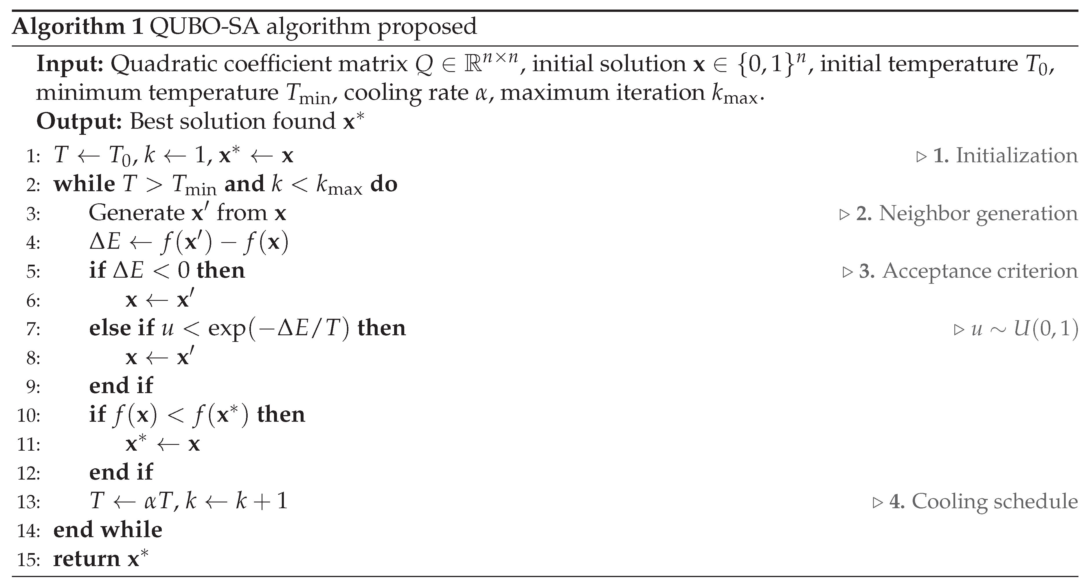
The QUBO-SA algorithm integrates these components into a unified iterative process. At each step, a candidate solution is generated from the current state and evaluated with respect to the QUBO objective. The acceptance rule balances diversification and intensification by allowing occasional uphill transitions, while improvements are tracked through the best-known solution . As the temperature parameter decreases, the search progressively shifts from broad exploration of the energy landscape toward focused refinement around promising regions. This combination of probabilistic exploration and controlled convergence defines the solver developed in this work.
4. Methods
This section describes the mathematical framework that underlies the proposed approach. We start by defining the Single-Pair Shortest Path problem in undirected weighted graphs, establishing the notation and structural constraints that define valid solutions. Following this, we adopt the QUBO formulation for the shortest path problem proposed by Krauss and McCollum [57], which consolidates both the path cost minimization objective and the structural validity constraints into a unified quadratic function over binary variables. Finally, we detail the algorithmic construction of the quadratic coefficient matrix Q, which enables the application of Simulated Annealing for efficient exploration of the solution space across diverse graph topologies.
4.1. Single-Pair Shortest Path Problem (SPSP)
Let represent an undirected graph, where is a finite set of vertices, is a set of edges, and is a set of real-valued edge costs associated with each edge . In this article, we assume that all edge costs are non-negative, i.e., for all , and therefore, negative edge costs are not considered.
In an undirected graph, the edges do not have a specific direction, meaning that if is an edge in the graph, then is also an edge. The connection between the vertices i and j is bidirectional.
A path in the graph from a node s to a node t is defined as a finite sequence of edges where each edge are adjacent. The shortest path problem involves finding such a sequence of edges starting at a source node s and ending at a target node t, where the starting node of the first edge in the sequence is the source point s, the arrival node of the last edge in the sequence is the target point t, and for each edge in the sequence, the arrival node of the previous edge is the same as the starting node of the next edge.
A path (P) from the source node s to the target node t can be expressed as:
where and . The total cost of P is determined by the sum of the weights of its constituent edges:
The objective of the shortest path problem is to find the path that minimizes the total cost .
It is important to note that the shortest path between two nodes is not necessarily unique. Multiple distinct paths may exist between the same pair of nodes such that , all of which would be considered optimal solutions satisfying . For example, as illustrated in Figure 1, consider a scenario where the graph contains two alternative paths: and . If both paths yield , then either constitutes a valid optimal solution.
The complexity of solving the shortest path problem can vary significantly depending on the structure of the graph and the nature of the edge costs. Classical algorithms deliver efficient polynomial-time solutions for numerous cases; however, problem complexity can escalate dramatically under more demanding scenarios, especially when dealing with additional constraints or large-scale graphs. Under such circumstances, advanced optimization techniques become necessary to overcome the computational challenges that arise.
4.2. QUBO Model Formulation
The SPSP problem can be expressed as a Quadratic Unconstrained Binary Optimization (QUBO) model, where both the path cost objective and structural feasibility requirements are jointly represented through a quadratic energy function defined over binary decision variables. This encoding approach utilizes linear coefficients for representing edge weights and quadratic penalty coefficients for enforcing topological constraints on the solution structure.
A valid path configuration needs to satisfy three essential requirements: (i) it must originate at the designated source node s, (ii) it must terminate at the specified target node t, and (iii) it must maintain edge connectivity throughout the entire path, thereby preventing fragmentation or branching at any vertex. To encode these conditions, the formulation uses binary variables, which are divided into node indicators representing intermediate vertices and edge indicators covering all graph connections.
The variable assignment follows a structured convention: each intermediate node corresponds to a binary indicator , while each edge is assigned a binary selector denoting its inclusion in the path. The vector therefore represents a complete system state:
where the source and target nodes are implicitly activated in all configurations. The objective function assumes the canonical QUBO form:
The cost component aggregates edge weights across the selected path:
while the constraint component enforces structural validity through three penalty mechanisms:
The penalty factor serves a critical function in ensuring that constraint violations dominate the objective value, effectively preventing infeasible solutions from being considered optimal. A properly calibrated penalty factor needs to satisfy , where denotes the cost of the shortest path. Given that remains unknown beforehand, we employ a conservative upper bound: , representing the sum of all edge costs in absolute value. This selection ensures that any configuration violating structural constraints receives a penalty that exceeds the maximum possible path cost, thereby effectively eliminating such configurations from consideration as optimal solutions. The scaling mechanism guarantees that the global minimum of corresponds exclusively to valid path structures exhibiting minimal cost.
The source constraint guarantees that precisely one edge is incident to the source node s:
where represents the neighborhood of s and by construction. This penalty function imposes the requirement that a valid path must begin from exactly one outgoing edge at the source vertex. Upon expansion, the quadratic term produces:
The leading negative term functions to compensate for the constant contribution when the constraint is met, yielding a global minimum of achieved precisely when . Any departure from this condition, whether through zero edges (disconnected path) or multiple edges (branching), raises the penalty value, thus discouraging such configurations during optimization. The quadratic structure guarantees that violations receive penalties proportional to their magnitude, with the squared difference amplifying deviations from the required degree.
The target constraint enforces a symmetric condition at the destination node t:
with expansion
where and denotes the neighborhood of t. This constraint ensures that the path concludes through exactly one incoming edge at the target vertex, mirroring the functionality of the source constraint. The minimum value of is reached when , thereby ensuring proper path termination. Similar to the source constraint, the negative quadratic offset modifies the baseline energy so that valid configurations produce negative contributions, whereas infeasible terminations, whether through no incoming edges or multiple simultaneous entries, incur positive penalties that render them ineligible for optimality.
The path continuity constraint guarantees that each intermediate vertex maintains connectivity through exactly two incident edges:
where each nodal contribution is expressed as
with explicit expansion
Here, encompasses all edges incident to node i. This constraint implements the essential principle that intermediate nodes on a simple path must display degree two: one edge for entrance and one for exit. When , the node is excluded from the path, and the penalty drops to zero provided no incident edges are selected (). In contrast, when , signaling inclusion in the path, the penalty is minimized at zero only when . Any violation, such as a degree-one node creating a dead end, or a degree-three (or higher) node causing branching, produces a positive penalty proportional to the squared deviation from the required degree. The summation across all intermediate vertices ensures that path continuity is enforced globally throughout the entire configuration. Taken together, the minimization of ensures that optimal configurations correspond to structurally valid paths connecting s to t without internal fragmentation or extraneous branches.
4.3. Algorithm Description
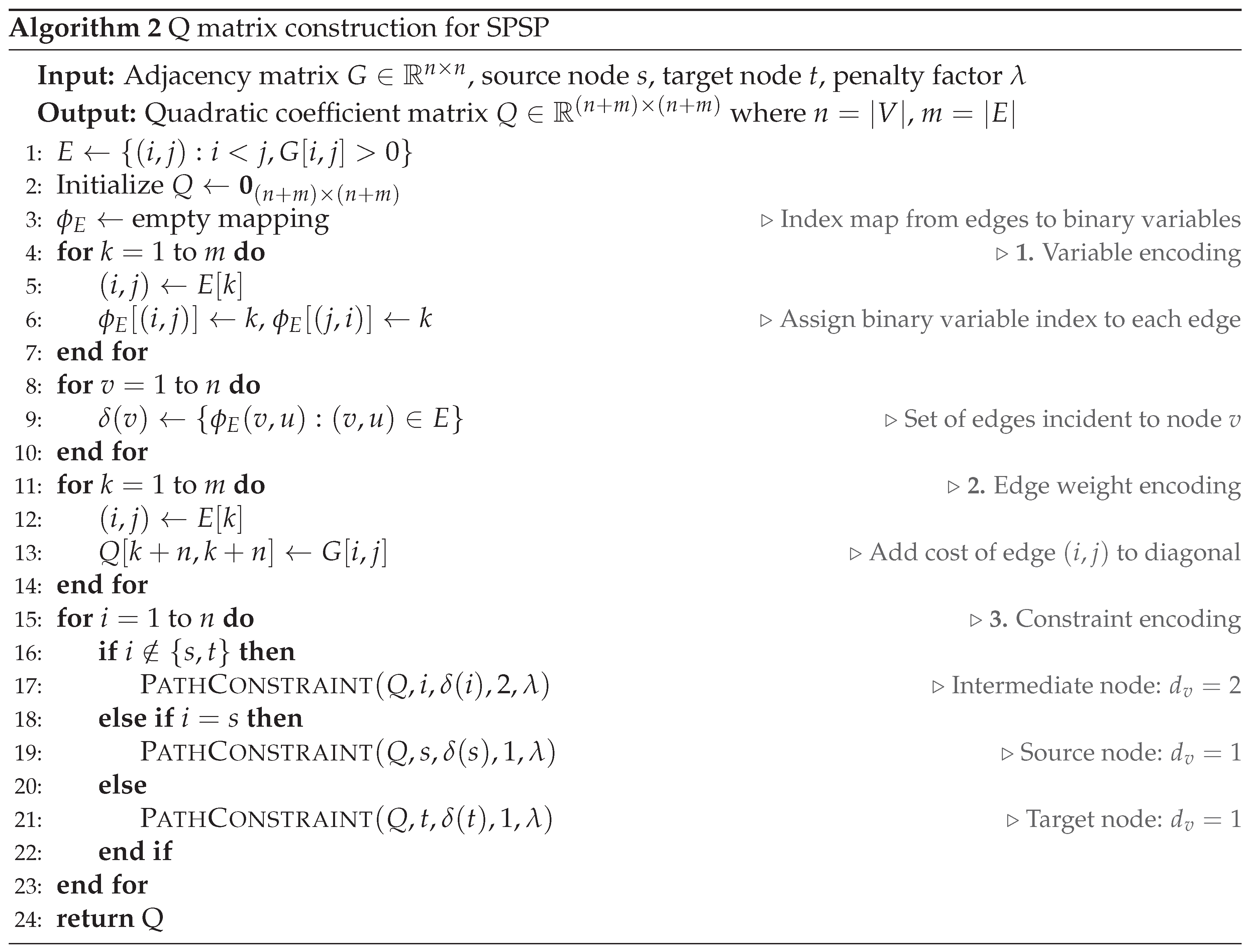
The construction of the quadratic coefficient matrix Q for the SPSP problem is achieved through a systematic process distributed across two algorithms. Algorithm 2 establishes the variable encoding and edge cost representation (), whereas Algorithm 3 enforces path validity through quadratic penalty terms corresponding to source and target nodes ( and ), intermediate nodes (), and general path continuity ().
The procedure in Algorithm 2 begins by creating a bijective mapping that associates each edge with a unique binary variable index. Given that the graph is undirected, both orientations and map to the same index. Simultaneously, for each node , the set of incident edge indices is compiled, enabling direct access to all edges connected to that vertex. This establishes the variables corresponding to nodes and edges, which will subsequently interact through the constraints. The variable vector incorporates binary variables for all vertices, including the source and destination nodes; later, are fixed through the penalty terms that enforce their activation within the feasible path.
Following index assignment, the edge costs are positioned on the diagonal entries , where . This encodes the path cost directly into the matrix as , ensuring that the total path length appears as the sum of selected edge variables.
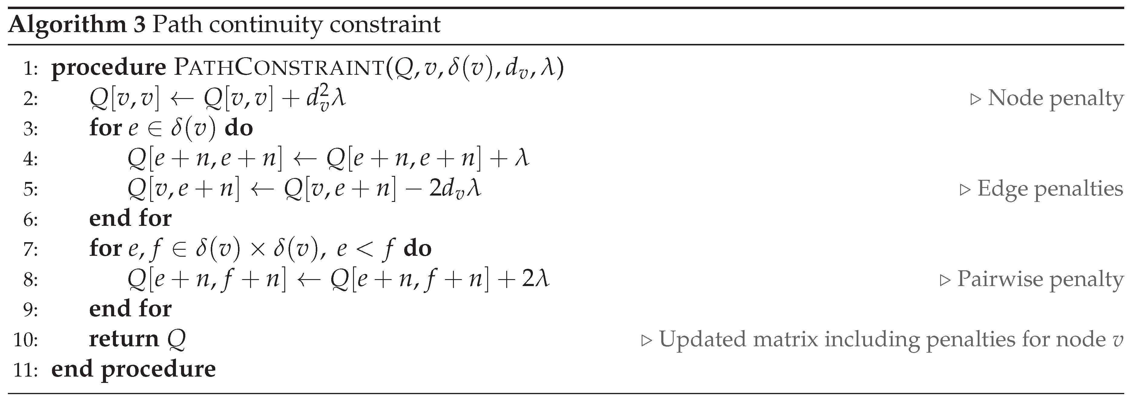
To guarantee structural validity of the path, constraints are implemented through Algorithm 3. Each node is handled according to its target degree: for the source node s and the target node t, and for intermediate nodes. These operations modify Q in-place, introducing quadratic and pairwise terms that realize the structural penalties included in . The resulting matrix Q now incorporates both the edge costs () and the node and edge penalty terms ().
Algorithm 3 implements the constraint enforcement mechanism. For a node v with target degree , three types of penalties are applied: (i) a quadratic penalty is added to (line 2), representing the cost of selecting the node itself; (ii) for each edge , the diagonal entry is incremented by , and the coupling is decremented by (lines 4–5), encouraging configurations that satisfy the node degree; (iii) for each pair of edges with , a pairwise term is added to (lines 7–9), penalizing configurations where multiple edges would violate the target degree. These penalties correspond to the components and , ensuring continuity and correct degree enforcement for each node.
5. Experimental Process and Results
This section describes the experimental framework and results obtained from evaluating the proposed QUBO-SA algorithm in comparison with the classical Dijkstra solver [16].
The comparison focuses on two main aspects: (i) solution reliability, captured through the empirical success probability , and (ii) computational efficiency, assessed using the Time-to-Solution () metric and the relative runtime ratio .
Computational Resources. All experiments were performed using Julia 1.11.5 on hardware equipped with an AMD Ryzen AI 9 HX 370 processor (12 cores / 24 threads, base clock 2.0 GHz) and 32 GB of RAM. No GPU acceleration was utilized.
5.1. Experimental Design and Evaluation Metrics
The evaluation procedure consists of three primary stages: graph preparation, QUBO encoding and optimization via simulated annealing (SA), and performance assessment based on probabilistic reliability. Both synthetic and real-world graph instances were employed to investigate how graph size and density affect solver behavior.
Graph preparation: Two categories of graph instances were considered:
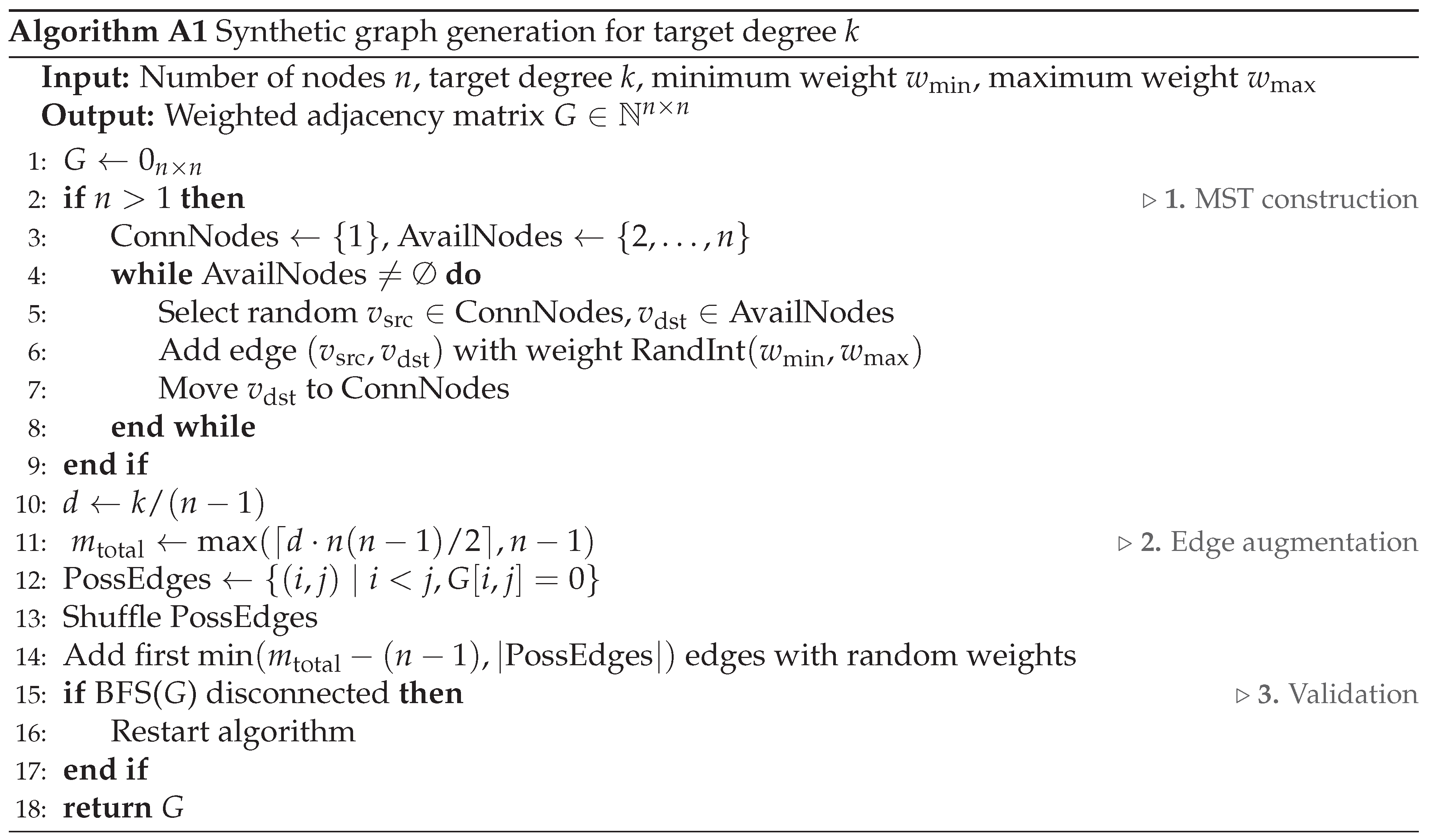
- Synthetic graphs: Undirected weighted graphs were constructed with a target average degree k, from which the corresponding density d is calculated. This parametrization facilitates systematic exploration of sparse (), moderately dense (), and dense () connectivity regimes across multiple node counts (). The complete generation procedure and pseudocode are detailed in Appendix A.
-
Urban Transportation Network.This real-world urban transportation network was derived from the downtown area of Querétaro City, México, a densely populated district with intricate routing demands arising from the coexistence of residential, commercial, and administrative zones. In this graph, nodes represent intersections or decision points, whereas edges denote bidirectional road segments weighted by geodesic distances calculated via the Haversine formula. The resulting network encapsulates realistic spatial constraints, including irregular connectivity patterns and hierarchical road organization characteristic of urban infrastructures.Figure 2 offers a representation of the study area: subfigure 2a positions Querétaro within its broader geographic context through a progressive zoom from national to municipal scale, whereas subfigure 2b illustrates the extracted network topology of the downtown area. In the latter, node coordinates match actual intersection positions obtained from OpenStreetMap data, and the designated source (green) and destination (blue) nodes were chosen to define a routing scenario that traverses multiple urban blocks, thereby encouraging path diversity across the sparse infrastructure.The extracted network contains nodes and edges, yielding an average degree of and a density of . This structural sparsity is typical of urban road systems, where intersections generally connect to only one or two neighboring streets, forming quasi-tree topologies. Such configurations impose a significant topological constraint on path diversity, thereby testing the capacity of the QUBO formulation to preserve connectivity continuity under limited redundancy.The routing scenario established for this network involves navigating 37 edges with an optimal path cost of 1,649 meters, representing the shortest valid route between the designated source and destination nodes. Table 1 summarizes the main topological and spatial characteristics of the Querétaro network that served as the real-world benchmark throughout the experimental evaluation.
QUBO-SA encoding and solver configuration
Each graph instance was transformed into a QUBO matrix following the formulation described in Section 4.2, where both the objective and constraint terms are incorporated within the quadratic cost coefficients. The optimization process adheres to the simulated annealing (SA) approach, as outlined in Algorithm 1, which utilizes a probabilistic acceptance of new states and a geometric cooling schedule. The solver parameters were calibrated as indicated in Table 2, guaranteeing consistent performance across different graph sizes.
Evaluation metrics
The performance assessment of the QUBO-SA solver depends on probabilistic indicators that capture both solution reliability and computational efficiency, recognizing the inherently stochastic character of simulated annealing. Instead of depending on single-run runtimes or best-case outcomes, we embrace a statistical framework where repeated executions yield an empirical success probability , defined as the proportion of runs that successfully recover the optimal path within the permitted iteration budget. This probability measures solver robustness and consistency across multiple trials, providing a more informative metric than isolated runtime values.
To relate this probabilistic measure to expected computational effort, we utilize the Time-to-Solution () metric [58,59,60,61], defined as:
where represents the average runtime per single QUBO-SA execution, and indicates the desired overall confidence of achieving an optimal solution at least once. Intuitively, estimates the expected total time necessary to reach a prescribed reliability level by considering the number of repetitions required to attain that success probability. A solver with high naturally produces smaller , whereas one with erratic convergence (low ) will display exponentially increasing values even when individual runs are fast.
In this study, we chose to represent high-confidence convergence aligned with standard benchmarks in stochastic optimization literature. Furthermore, we report values for to reveal the trade-off between reliability and computational efficiency: lowering the target confidence typically reduces , indicating that slightly less stringent reliability requirements can result in substantial runtime savings.
For comparative evaluation, the deterministic Dijkstra algorithm functions as the baseline reference, supplying a mean runtime calculated over 100 independent executions. This enables the definition of the relative runtime ratio:
which expresses the time required by the probabilistic solver to reach a given confidence level relative to the runtime of the deterministic benchmark. By normalizing both runtimes, R provides a scale-invariant comparison across heterogeneous graph instances and hardware environments: indicates that QUBO-SA attains the desired reliability faster than Dijkstra, whereas implies additional computational effort to achieve equivalent confidence.
5.2. Comparative Performance Across Graph Regimes
Table 3 summarizes the relative runtime ratios and across synthetic and urban networks. Confidence intervals () were obtained by propagating the binomial uncertainty of through the definition.
The synthetic benchmarks reveal a clear progression from near-trivial reliability at small scales to increasingly costly convergence as n grows. For , the solver attains in two of three configurations, collapsing to zero and yielding ; even in the less favorable case (, ), remains at 0.5 with modest overhead relative to Dijkstra. By , success probabilities drop into the 0.82–0.90 range and increases to values between 65 and 185 , pushing into 2.09–2.82. This trend intensifies at and , where drops to 0.53–0.74 and increases to values between 1,310 and 4,950 , producing – with expanding confidence intervals, demonstrating that large instances amplify stochastic variability and the number of repetitions required for high-confidence convergence. Across all sizes, lowering the target from to 0.90 consistently decreases runtime by approximately a factor of two (), suggesting that the primary cost stems from enhancing reliability rather than from single-run execution time. Taken together, the scaling with n and the associated decrease in d for fixed k constrain feasible path redundancy and hinder annealing transitions, shifting synthetic graphs from a regime of effectively deterministic recovery at small n to one where robustness requires exponentially more repetitions as n increases.
For the Querétaro urban transportation network (, ), the solver reached a success probability of , which translates into a of 9,250 compared to 6,850 for Dijkstra. The resulting runtime ratio of shows that QUBO-SA requires about one third more time than the deterministic baseline to guarantee 99% confidence. When the confidence level is reduced to , the ratio decreases to , revealing that most of the additional cost is focused on achieving very high reliability rather than on generating an optimal solution per se. This behavior aligns with the synthetic benchmarks, where the gap between and also captures the trade-off between robustness and efficiency.
Figure 3 displays the optimal 37-edge path of total cost 1,649 m, linking the source and target nodes across the urban district.
The structural characteristics of the urban graph help clarify these results. Its low density () diminishes the number of feasible paths, which simplifies constraint satisfaction but also restricts redundancy, making it more challenging for the annealing process to escape local minima. Nevertheless, the observed runtime ratios remain competitive. Despite the substantially larger scale (), the solver’s performance is comparable to that of synthetic graphs with , where ranges from to . This suggests that the spatial organization of real road networks, characterized by clustering around intersections and hierarchical arterial structures, introduces regularities that partially compensate for the computational burden of size, enabling QUBO-SA to navigate the solution space more efficiently than in purely random topologies.
5.3. Further Works
The experimental results described in this study reveal several promising avenues for future research. The neighbor generation mechanism in the current QUBO-SA implementation employs a simple bit-flip strategy, which may limit the efficiency of exploration in large solution spaces. An adaptive neighbor generation scheme that dynamically modifies the perturbation intensity based on search progress could substantially improve convergence rates. This mechanism could incorporate multiple neighborhood structures, choosing among them based on the current temperature regime or recent acceptance history, thereby strengthening the balance between diversification and intensification throughout the annealing schedule.
The penalty factor is essential for guaranteeing constraint satisfaction. However, its current definition as the sum of all edge costs functions as a conservative upper bound that may introduce unnecessary numerical scaling in heterogeneous graphs. Performing a systematic sensitivity analysis to examine the relationship between , graph structure, and solution quality would yield valuable insights into optimal penalty calibration strategies. This analysis should investigate how different penalty scaling approaches influence both feasibility enforcement and convergence speed across graphs with varying cost distributions.
The QUBO formulation naturally extends to quantum annealing platforms, where the quadratic structure can be directly mapped onto quantum processing units, such as those manufactured by D-Wave Systems. Empirical evaluation on quantum hardware would permit a direct comparison of thermal and quantum annealing dynamics for the Shortest Path Selection Problem (SPSP), potentially uncovering quantum advantages in specific graph regimes or problem scales. Such an investigation would need to address hardware connectivity constraints, embedding overhead carefully, and the noise characteristics inherent to current quantum annealers.
6. Conclusions
This work has assessed the performance of a QUBO-based Simulated Annealing approach for solving the Single-Pair Shortest Path problem across diverse graph topologies. The experimental evaluation included synthetic graphs with controlled connectivity regimes spanning from sparse to dense configurations, alongside a real-world urban transportation network. Results indicate that the QUBO-SA framework achieves competitive performance relative to classical deterministic algorithms when reliability requirements are adjusted to practical confidence levels. For small synthetic instances, the solver reached near-perfect success rates with minimal overhead, whereas larger graphs displayed reduced success probabilities requiring additional computational effort to ensure high-confidence convergence. The urban network evaluation showed that structural characteristics of real-world graphs, including spatial clustering and hierarchical organization, partially offset the computational burden associated with problem scale, producing performance comparable to moderately sized synthetic instances despite significantly larger node counts.
The probabilistic nature of the solver introduces a fundamental trade-off between solution reliability and computational efficiency, as measured through the Time-to-Solution metric. Reducing the target confidence from 99% to 90% consistently lowered runtime overhead by approximately half across all tested configurations, demonstrating that most computational cost originates from achieving very high reliability rather than from the intrinsic difficulty of finding optimal solutions. This characteristic renders the approach particularly suitable for applications where occasional suboptimal solutions are acceptable or where multiple independent runs can be executed in parallel. Future work exploring adaptive neighborhood strategies, penalty calibration techniques, quantum hardware implementations, and alternative metaheuristic solvers will further clarify the practical boundaries of this approach and identify the specific problem regimes where QUBO-based optimization offers genuine advantages over traditional methods.
Author Contributions
Conceptualization, I.O.-G. and H.J.-H.; formal analysis, I.O.-G. and H.J.-H.; investigation, I.O.-G. and H.J.-H.; methodology, I.O.-G. and H.J.-H.; software, I.O.-G.; supervision, H.J.-H.; validation, H.J.-H.; writing—original draft preparation, I.O.-G. and H.J.-H.; writing—review and editing, I.O.-G. and H.J.-H.
Funding
This research received no external funding
Data Availability Statement
The original contributions presented in this study are included in the article. Further inquiries can be directed to the corresponding author.
Conflicts of Interest
The authors declare no conflicts of interest.
Appendix A. Synthetic Graph Generation Algorithm
Synthetic undirected weighted graphs are constructed with a predefined target average degree k, from which the corresponding edge density is calculated as
This formulation enables connectivity to be regulated directly through k, whereas d serves as a derived measure for interpreting the resulting topologies. Three connectivity levels are examined: (sparse), (moderate), and (dense), ensuring that the influence of n is isolated from local connectivity. The generation process yields instances that are both connected and precisely aligned with the desired k, facilitating fair comparisons across sizes and connectivity regimes. For each configuration:
- 1.
- Minimum Spanning Tree (MST) construction: Initialize an undirected graph with n nodes. Iteratively introduce edges to form an MST, ensuring edges and global connectivity, with integer weights drawn from .
- 2.
- Edge augmentation: Computeand randomly add non-existing edges until achieving this count, assigning weights within the same range.
- 3.
- Validation: Confirm connectivity via a Breadth-First Search (BFS). If the graph is disconnected, repeat the generation to guarantee valid inputs for the evaluation framework in Section 4.2.
This procedure guarantees that the desired average degree k is consistently attained, prevents disconnected components, and preserves comparable connectivity conditions across experimental settings.
References
- Tu, Q.; Cheng, L.; Yuan, T.; Cheng, Y.; Li, M. The constrained reliable shortest path problem for electric vehicles in the urban transportation network. Journal of cleaner production 2020, 261, 121130.
- Koritsoglou, K.; Tsoumanis, G.; Patras, V.; Fudos, I. Shortest Path Algorithms for Pedestrian Navigation Systems. Information 2022, 13. [CrossRef]
- Liu, J.; Gu, H.; Wei, W.; Chen, Z.; Chen, Y. An efficient shortest path algorithm for content-based routing on 2-D mesh accelerator networks. Future Generation Computer Systems 2021, 114, 519–530.
- Lyu, D.; Chen, Z.; Cai, Z.; Piao, S. Robot path planning by leveraging the graph-encoded Floyd algorithm. Future Generation Computer Systems 2021, 122, 204–208. [CrossRef]
- WU, X.; XIAO, B.; WU, C.; GUO, Y.; LI, L. Factor graph based navigation and positioning for control system design: A review. Chinese Journal of Aeronautics 2022, 35, 25–39. [CrossRef]
- Alamsyah, A.; Rahardjo, B.; et al. Social network analysis taxonomy based on graph representation. arXiv preprint arXiv:2102.08888 2021.
- Brambilla, M.; Javadian Sabet, A.; Kharmale, K.; Sulistiawati, A.E. Graph-based conversation analysis in social media. Big Data and Cognitive Computing 2022, 6, 113.
- Yi, H.C.; You, Z.H.; Huang, D.S.; Kwoh, C.K. Graph representation learning in bioinformatics: trends, methods and applications. Briefings in Bioinformatics 2022, 23, bbab340.
- Liu, M.; Li, X.; Li, J.; Liu, Y.; Zhou, B.; Bao, J. A knowledge graph-based data representation approach for IIoT-enabled cognitive manufacturing. Advanced Engineering Informatics 2022, 51, 101515.
- Saha, S.; Gao, J.; Gerlach, R. A survey of the application of graph-based approaches in stock market analysis and prediction. International Journal of Data Science and Analytics 2022, 14, 1–15.
- Sihotang, H.T.; Riandari, F.; Sihotang, J. Graph-based Exploration for Mining and Optimization of Yields (GEMOY Method). Jurnal Teknik Informatika CIT Medicom 2024, 16, 70–81.
- Jalving, J.; Shin, S.; Zavala, V.M. A graph-based modeling abstraction for optimization: Concepts and implementation in plasmo. jl. Mathematical Programming Computation 2022, 14, 699–747.
- Hua, R.; Dinneen, M.J. Improved QUBO formulation of the graph isomorphism problem. SN Computer Science 2020, 1, 1–18.
- Lucas, A. Ising formulations of many NP problems. Frontiers in physics 2014, 2, 5.
- Krauss, T.; McCollum, J.; Pendery, C.; Litwin, S.; Michaels, A.J. Solving the max-flow problem on a quantum annealing computer. IEEE Transactions on Quantum Engineering 2020, 1, 1–10.
- Dijkstra, E.W. A note on two problems in connexion with graphs. Numerische Mathematik 1959, 1, 269–271. [CrossRef]
- Shier, D.R. A computational study of Floyd’s algorithm. Computers & Operations Research 1981, 8, 275–293.
- Hart, P.E.; Nilsson, N.J.; Raphael, B. A Formal Basis for the Heuristic Determination of Minimum Cost Paths. IEEE Transactions on Systems Science and Cybernetics 1968, 4, 100–107. [CrossRef]
- Li, L.; Gu, Q.; Liu, L. Research on path planning Algorithm for Multi-UAV Maritime Targets Search Based on Genetic Algorithm. In Proceedings of the Proceedings of the 2020 IEEE International Conference on Information Technology, Big Data and Artificial Intelligence (ICIBA), Chongqing, China, 6–8 November 2020; pp. 840–843.
- Elhoseny, M.; Tharwat, A.; Hassanien, A. Bezier Curve Based Path Planning in a Dynamic Field using Modified Genetic Algorithm. Journal of Computational Science 2018, 25, 339–350.
- Yu, L.; Wei, Z.; Wang, H.; Ding, Y.; Wang, Z. Path planning for mobile robot based on fast convergence ant colony algorithm. In Proceedings of the 2017 IEEE International Conference on Mechatronics and Automation (ICMA), Takamatsu, Japan, 2017; pp. 1493–1497.
- Çalık, S. UAV path planning with multiagent Ant Colony system approach. In Proceedings of the Signal Processing and Communications Applications (SIU), Zonguldak, Turkey, 2016; pp. 1409–1412.
- Ding, F.; Zhang, Z.; Fu, M.; Wang, Y.; Wang, C. Energy-Efficient Path Planning and Control Approach of USV Based on Particle Swarm Optimization. In Proceedings of the OCEANS MTS/IEEE Charleston, Charleston, SC, USA, 2018; pp. 1–6.
- Phung, M.; Ha, Q. Safety-enhanced UAV path planning with spherical vector-based particle swarm optimization. Applied Soft Computing 2021, 107, 107376.
- Ma, B.; He, Y.; Du, J.; Han, M. Research on path planning Problem of Optical Fiber Transmission Network Based on Simulated Annealing Algorithm. In Proceedings of the 2019 IEEE 8th Joint International Information Technology and Artificial Intelligence Conference (ITAIC), Chongqing, China, 2019; pp. 1298–1301.
- Yin, J.; Fu, W. A Hybrid Path Planning Algorithm Based on Simulated Annealing Particle Swarm for The Self-driving Car. In Proceedings of the 2018 International Computers, Signals and Systems Conference (ICOMSSC), Dalian, China, 2018; pp. 696–700.
- Liu, K.; Zhang, M. Path Planning Based on Simulated Annealing Ant Colony Algorithm. In Proceedings of the 2016 9th International Symposium on Computational Intelligence and Design (ISCID), Hangzhou, China, 2016; pp. 461–466.
- Yue, X.; Zhang, W. UAV path planning Based on K-Means Algorithm and Simulated Annealing Algorithm. In Proceedings of the 2018 37th Chinese Control Conference (CCC), Wuhan, China, 2018; pp. 2290–2295.
- Krause, T.; McCallum, J. Solving the network shortest path problem on a quantum annealer. IEEE Transactions on Quantum Engineering 2020, 1, 1–12.
- Ge, F.; Li, K.; Xu, W.; Wang, Y. Path Planning of UAV for Oilfield Inspection Based on Improved Grey Wolf Optimization Algorithm. In Proceedings of the 31st Chinese Control and Decision Conference, NanChang, China, 2019; pp. 3666–3671.
- Wu, C.; Huang, X.; Luo, Y.; Leng, S. An Improved Fast Convergent Artificial Bee Colony Algorithm for Unmanned Aerial Vehicle Path Planning Battlefield Environment. In Proceedings of the 2020 IEEE International Conference on Control & Automation (ICCA), Singapore, 2020; pp. 360–365.
- Tian, G.; Zhang, L.; Bai, X.; Wang, B. Real-time Dynamic Track Planning of Multi-UAV Formation Based on Improved Artificial Bee Colony Algorithm. In Proceedings of the 2018 37th Chinese Control Conference (CCC), Wuhan, China, 2018; pp. 10055–10060.
- Duan, H.; Li, S. Artificial bee colony–based direct collocation for reentry trajectory optimization of hypersonic vehicle. IEEE Transactions on Aerospace and Electronic Systems 2015, 51, 615–626.
- Balan, K.; Luo, C. Optimal Trajectory Planning for Multiple Waypoint Path Planning using Tabu Search. In Proceedings of the 2018 9th IEEE Annual Ubiquitous Computing, Electronics & Mobile Communication Conference (UEMCON), New York, NY, USA, 2018; pp. 497–501.
- Rabbouch, B.; Rabbouch, H.; Saâdaoui, F.; Mraihi, R. Chapter 22 - Foundations of combinatorial optimization, heuristics, and metaheuristics. In Comprehensive Metaheuristics; Mirjalili, S.; Gandomi, A.H., Eds.; Academic Press, 2023; pp. 407–438. [CrossRef]
- Punnen, A.P. The quadratic unconstrained binary optimization problem. Springer International Publishing 2022, 10, 978–3.
- Quintero, R.A.; Zuluaga, L.F. QUBO Formulations of Combinatorial Optimization Problems for Quantum Computing Devices. In Encyclopedia of Optimization; Springer, 2022; pp. 1–13.
- Cormen, T.H.; Leiserson, C.E.; Rivest, R.L.; Stein, C. Introduction to algorithms; MIT press, 2022.
- Fredman, M.L.; Tarjan, R.E. Fibonacci heaps and their uses in improved network optimization algorithms. Journal of the ACM (JACM) 1987, 34, 596–615.
- Driscoll, J.R.; Gabow, H.N.; Shrairman, R.; Tarjan, R.E. Relaxed heaps: an alternative to Fibonacci heaps with applications to parallel computation. Commun. ACM 1988, 31, 1343–1354. [CrossRef]
- Gabow, H.N.; Tarjan, R.E. Algorithms for two bottleneck optimization problems. Journal of Algorithms 1988, 9, 411–417. [CrossRef]
- Duan, R.; Lyu, K.; Wu, H.; Xie, Y. Single-Source Bottleneck Path Algorithm Faster than Sorting for Sparse Graphs, 2018, [arXiv:cs.DS/1808.10658].
- Williams, V.V. Nondecreasing paths in a weighted graph or: How to optimally read a train schedule. ACM Trans. Algorithms 2010, 6. [CrossRef]
- Duan, R.; Mao, J.; Mao, X.; Shu, X.; Yin, L. Breaking the Sorting Barrier for Directed Single-Source Shortest Paths. In Proceedings of the Proceedings of the 57th Annual ACM Symposium on Theory of Computing (STOC), New York, NY, USA, 2025; pp. 36–44.
- Pettie, S.; Ramachandran, V. A Shortest Path Algorithm for Real-Weighted Undirected Graphs. SIAM Journal on Computing 2005, 34, 1398–1431. [CrossRef]
- chih Yao, A.C. An 0(|E|loglog|V|) algorithm for finding minimum spanning trees. Information Processing Letters 1975, 4, 21–23. [CrossRef]
- Dürr, C.; Heiligman, M.; HOyer, P.; Mhalla, M. Quantum query complexity of some graph problems. SIAM Journal on Computing 2006, 35, 1310–1328.
- Belovs, A.; Reichardt, B.W. Span programs and quantum algorithms for st-connectivity and claw detection. In Proceedings of the European Symposium on Algorithms. Springer, 2012, pp. 193–204.
- Belovs, A. Quantum walks and electric networks. arXiv preprint arXiv:1302.3143 2013.
- Jeffery, S.; Kimmel, S.; Piedrafita, A. Quantum algorithm for path-edge sampling. arXiv preprint arXiv:2303.03319 2023.
- Wesołowski, A.; Piddock, S. Advances in quantum algorithms for the shortest path problem. arXiv preprint arXiv:2408.10427 2024. bounded-error quantum algorithms in adjacency list model: and .
- Ashvinkumar, V.; Bernstein, A.; Cao, N.; Grunau, C.; Haeupler, B.; Jiang, Y.; Nanongkai, D.; Su, H.H. Parallel, Distributed, and Quantum Exact Single-Source Shortest Paths with Negative Edge Weights. In Proceedings of the 32nd Annual European Symposium on Algorithms (ESA 2024). Dagstuhl–Leibniz-Zentrum für Informatik, 2024, Vol. 308, Leibniz International Proceedings in Informatics (LIPIcs), pp. 13:1–13:15. [CrossRef]
- Pardalos, P.M.; Jha, S. Complexity of uniqueness and local search in quadratic 0–1 programming. Operations research letters 1992, 11, 119–123.
- Karp, R.M. Reducibility among combinatorial problems; Springer, 2010.
- Kirkpatrick, S.; Gelatt Jr, C.D.; Vecchi, M.P. Optimization by simulated annealing. science 1983, 220, 671–680.
- Metropolis, N.; Rosenbluth, A.W.; Rosenbluth, M.N.; Teller, A.H.; Teller, E. Equation of state calculations by fast computing machines. The journal of chemical physics 1953, 21, 1087–1092.
- Krauss, T.; McCollum, J. Solving the network shortest path problem on a quantum annealer. IEEE Transactions on Quantum Engineering 2020, 1, 1–12.
- Mohseni, N.; McMahon, P.L.; Byrnes, T. Ising machines as hardware solvers of combinatorial optimization problems. Nature Reviews Physics 2022, 4, 363–379.
- Aramon, M.; Rosenberg, G.; Valiante, E.; Miyazawa, T.; Tamura, H.; Katzgraber, H.G. Physics-Inspired Optimization for Quadratic Unconstrained Problems Using a Digital Annealer. Frontiers in Physics 2019, 7. [CrossRef]
- Rønnow, T.F.; Wang, Z.; Job, J.; Boixo, S.; Isakov, S.V.; Wecker, D.; Martinis, J.M.; Lidar, D.A.; Troyer, M. Defining and detecting quantum speedup. Science 2014, 345, 420–424. [CrossRef]
- Zielewski, M.R.; Takizawa, H. A method for reducing time-to-solution in quantum annealing through pausing. In Proceedings of the International Conference on High Performance Computing in Asia-Pacific Region, 2022, pp. 137–145.
Figure 1.
Example of an undirected weighted graph showing two distinct optimal paths of equal cost between nodes and .
Figure 1.
Example of an undirected weighted graph showing two distinct optimal paths of equal cost between nodes and .
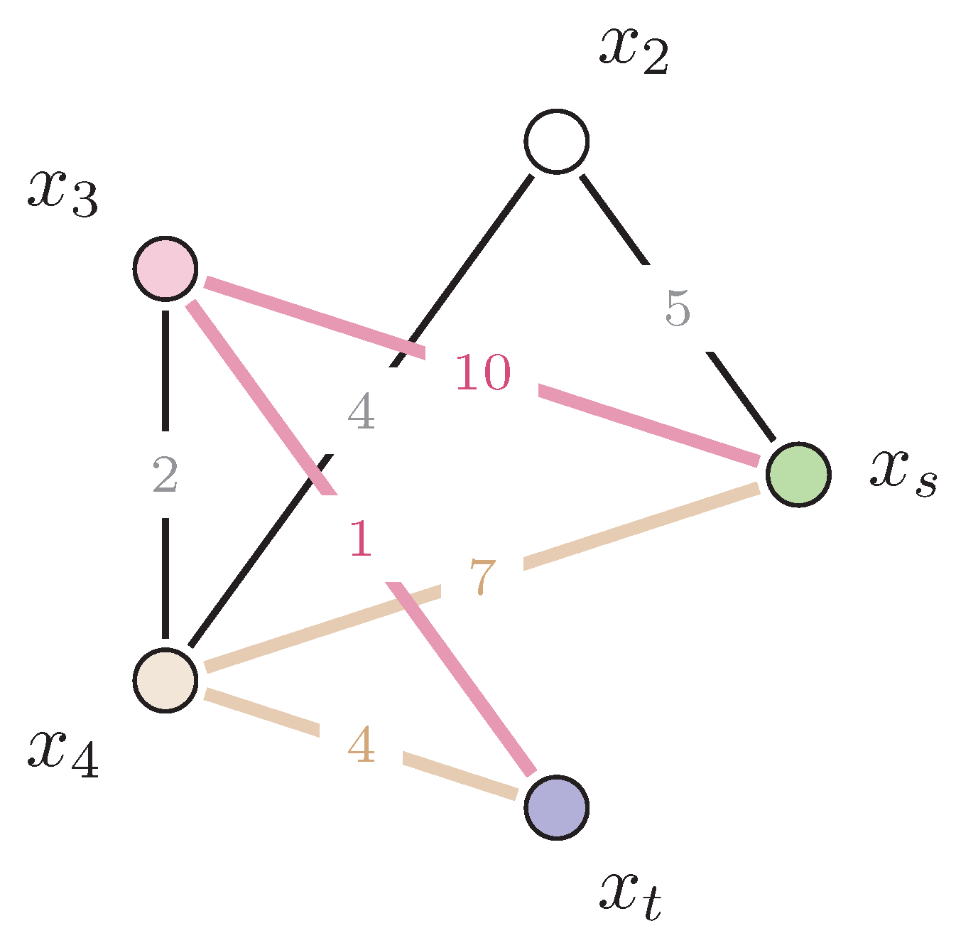
Figure 2.
Querétaro urban transportation network: (a) geographic contextualization from national to municipal scale; (b) extracted downtown topology with source (green) and destination (blue) nodes.
Figure 2.
Querétaro urban transportation network: (a) geographic contextualization from national to municipal scale; (b) extracted downtown topology with source (green) and destination (blue) nodes.
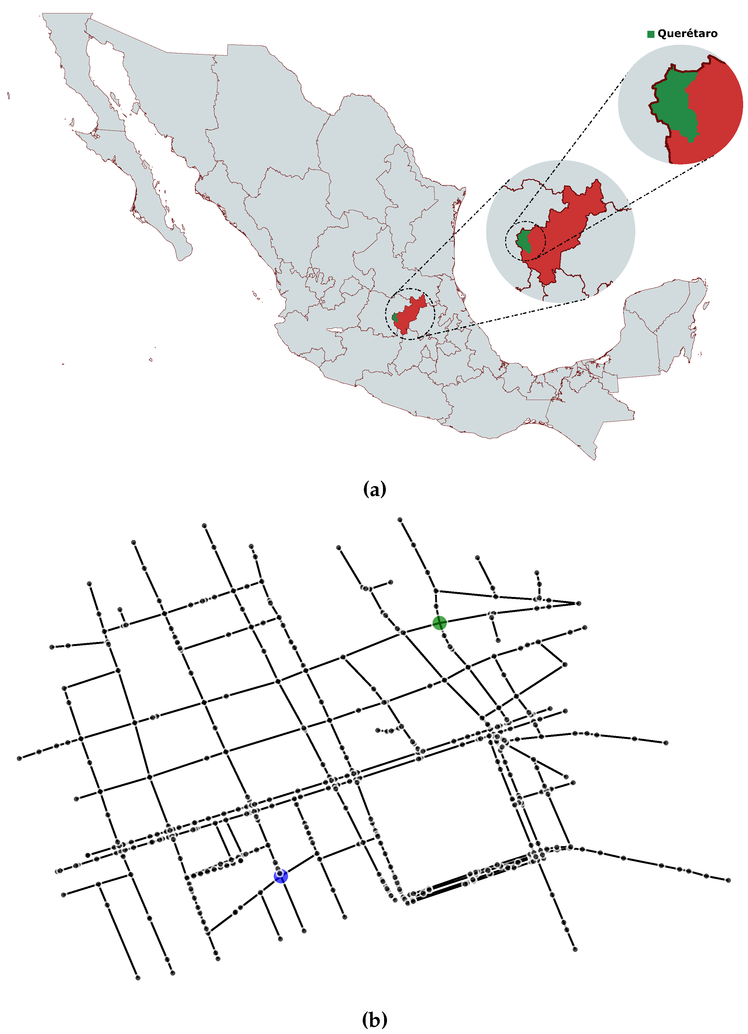
Figure 3.
Optimal path (highlighted in red) identified by QUBO-SA for the routing scenario on the Querétaro urban network. The path connects the source node (green) to the target node (blue) with a total cost of 1,649 meters across 37 edges.
Figure 3.
Optimal path (highlighted in red) identified by QUBO-SA for the routing scenario on the Querétaro urban network. The path connects the source node (green) to the target node (blue) with a total cost of 1,649 meters across 37 edges.
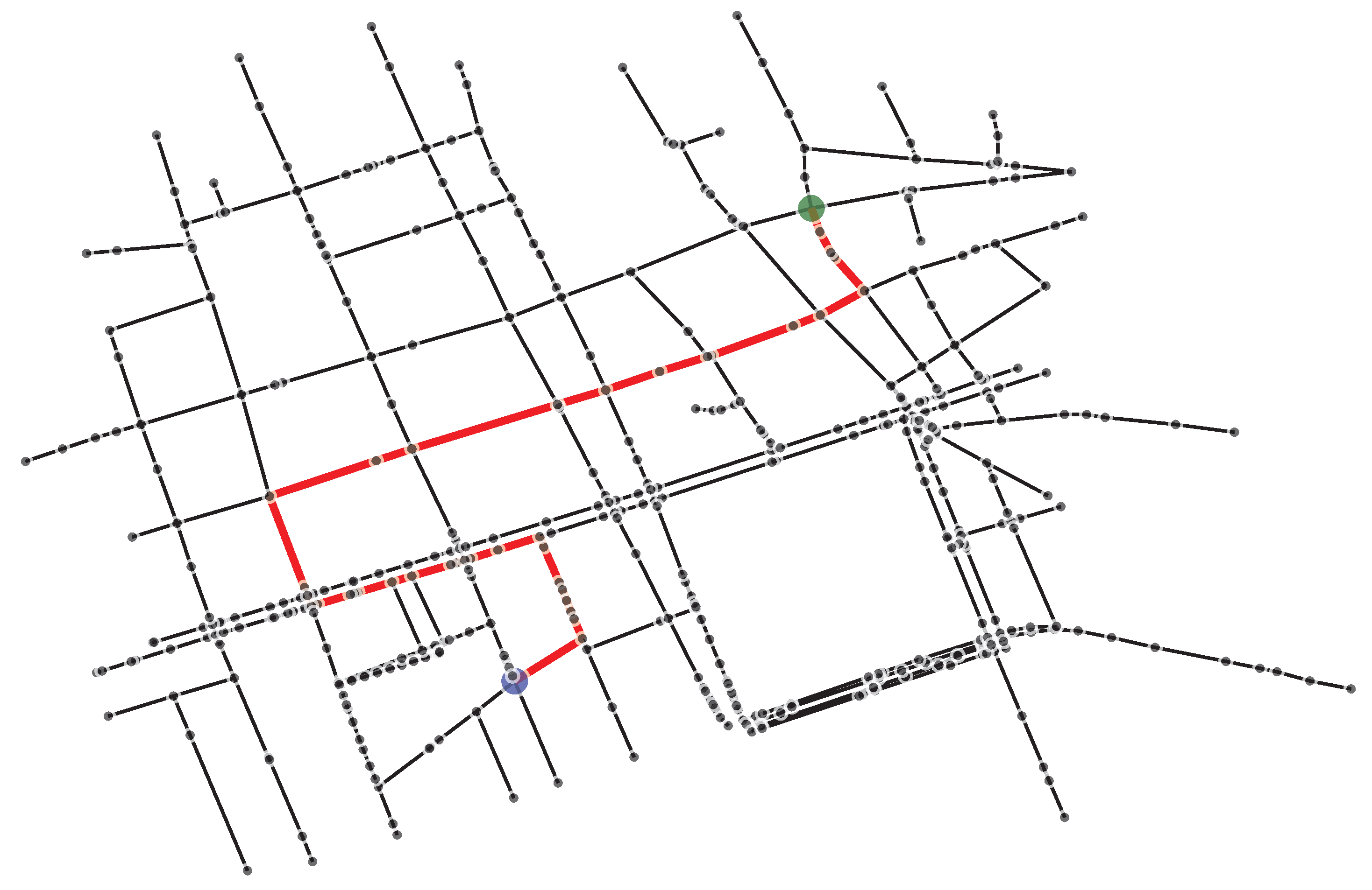

Table 1.
Structural and routing characteristics of the Querétaro urban transportation network.
| Property | Value |
|---|---|
| Network Properties | |
| Number of nodes (n) | 443 |
| Number of edges (m) | 245 |
| Average degree (k) | 1.11 |
| Graph density (d) | 0.25% |
| Connected components | 1 (fully connected) |
| Average shortest-path length | 27.3 edges |
| Routing Scenario | |
| Source node | Northeastern sector |
| Destination node | Southeastern sector |
| Optimal path length | 37 edges |
| Optimal path cost | 1,649 m |
| Average edge length | 44.6 m |
| Maximum node degree | 3 |
Note. All graph indicators were derived after preprocessing the OpenStreetMap data with LightOSM.jl. The routing scenario was designed to cross the downtown area across multiple urban sectors, ensuring representative coverage of the structural characteristics of the network.
Table 2.
QUBO-SA algorithm parameters.
| Parameter | Symbol | Value | Description |
|---|---|---|---|
| Initial temperature | Adaptive scaling to graph size | ||
| Cooling rate | Geometric cooling schedule | ||
| Maximum iterations | Termination criterion | ||
| Penalty factor | Sum of absolute edge costs |
Note. and are most influential: higher promotes exploration, whereas yields smoother cooling at the cost of longer runs. The penalty factor ensures constraint feasibility by scaling penalties proportionally to edge magnitudes.
Table 3.
Comparative performance of QUBO-SA and Dijkstra across synthetic and urban networks.
| n | k | d | (s) | (s) | (s) | (↓, ↑) | |||
|---|---|---|---|---|---|---|---|---|---|
| Synthetic Graphs | |||||||||
| 10 | 1 | 0.111 | 1.00 | 11.8 | 12.0 | 11.5 | 0.00 | – | 0.00 |
| 2 | 0.222 | 1.00 | 7.3 | 7.5 | 7.2 | 0.00 | – | 0.00 | |
| 3 | 0.333 | 0.97 | 0.49 | 0.50 | 0.48 | 1.37 | (0.17, 1.74) | 0.68 | |
| 20 | 1 | 0.053 | 0.85 | 182.0 | 185.0 | 178.0 | 2.52 | (1.90, 3.16) | 1.26 |
| 2 | 0.105 | 0.90 | 118.0 | 120.0 | 115.0 | 2.09 | (1.66, 2.68) | 1.04 | |
| 3 | 0.158 | 0.82 | 63.0 | 65.0 | 62.0 | 2.82 | (2.03, 3.28) | 1.41 | |
| 30 | 1 | 0.034 | 0.68 | 1,920.0 | 1,950.0 | 1,870.0 | 4.21 | (3.28, 5.01) | 2.11 |
| 2 | 0.069 | 0.74 | 1,560.0 | 1,580.0 | 1,520.0 | 3.55 | (2.76, 4.56) | 1.78 | |
| 3 | 0.103 | 0.62 | 1,290.0 | 1,310.0 | 1,380.0 | 4.52 | (3.46, 5.81) | 2.26 | |
| 40 | 1 | 0.026 | 0.56 | 4,920.0 | 4,950.0 | 5,120.0 | 5.42 | (4.21, 6.84) | 2.71 |
| 2 | 0.051 | 0.61 | 3,650.0 | 3,675.0 | 3,820.0 | 4.71 | (3.62, 6.13) | 2.35 | |
| 3 | 0.077 | 0.53 | 2,860.0 | 2,890.0 | 3,010.0 | 5.86 | (4.47, 7.81) | 2.93 | |
| Urban Transportation Network | |||||||||
| 443 | 1.11 | 0.0025 | 0.57 | 9,100 | 9,250 | 6,850 | 1.35 | (1.05, 1.72) | 1.08 |
Notes. denotes the mean runtime per QUBO–SA execution (100 repetitions). and represent the relative runtime ratios for target confidences and , respectively. corresponds to a 95% confidence interval propagated from the binomial uncertainty in . Rows with show very small (nonzero) values, as all runs converged to the optimal solution. Symbols ↓ and ↑ denote the lower and upper bounds of the confidence interval.
Disclaimer/Publisher’s Note: The statements, opinions and data contained in all publications are solely those of the individual author(s) and contributor(s) and not of MDPI and/or the editor(s). MDPI and/or the editor(s) disclaim responsibility for any injury to people or property resulting from any ideas, methods, instructions or products referred to in the content. |
© 2025 by the authors. Licensee MDPI, Basel, Switzerland. This article is an open access article distributed under the terms and conditions of the Creative Commons Attribution (CC BY) license (http://creativecommons.org/licenses/by/4.0/).
Copyright: This open access article is published under a Creative Commons CC BY 4.0 license, which permit the free download, distribution, and reuse, provided that the author and preprint are cited in any reuse.


