
Submitted:
06 November 2025
Posted:
10 November 2025
You are already at the latest version
Abstract
To address the issues of inefficiency and high costs in obtaining data on the residential distribution of public transport passengers at present, this paper proposes an approach of "estimating the residential distribution of public transport passengers based on characteristics such as housing prices of residential Point of Interest (POI) and the convenience of public transport and its stops". First, from two aspects—public transport travel and the selection of public transport stops—eight influencing factors for the selection of public transport stops during travel are identified. Based on these factors, a regression model for the number of public transport passengers from residential POI to their corresponding stops is constructed, through which the number of passengers traveling from each residential POI to all accessible public transport stops is obtained. This number is then used as a weight to allocate the actual passenger flow of each public transport stop to respective residential POI, thereby realizing the estimation of the residential distribution of public transport passengers. Furthermore, this approach enables the estimation of the proportion of trips made from residential areas to specific public transport stops and the overall proportion of public transport trips among all travel modes from residential areas. The proposed estimation method is verified and evaluated using Shenzhen as a case study. The results show that the Mean Absolute Percentage Error (MAPE) of the proposed model is 72.024%, which outperforms the XGBoost model that uses the same set of characteristics.
Keywords:
proportion of trips to public transport stops
; web crawler
; regression model
1. Introduction
In recent years, with the large-scale construction of urban rail transit and the diversification of transportation modes, the development of conventional public transport has been confronted with unprecedented challenges and pressures. From 2019 to 2024, the annual passenger volume of conventional public transport across the country decreased from 69.176 billion person-times to 38.670 billion person-times, with a decline rate of 44.1%. Faced with the new transportation situation, the development of conventional public transport should change traditional thinking, actively promote the supply-side reform of conventional public transport services, and shift from the previous focus on increasing the "quantity" of supply—such as simply expanding the density of the route network and the frequency of departures—to enhancing the "quality" of public transport services.
Mastering accurate passenger travel demand is a prerequisite for improving public transport service quality. Currently, the technology for estimating public transport passengers' OD (Origin-Destination) data is relatively mature, but its accuracy is not high—it can only estimate data down to the level of public transport stops. However, achieving improvements in the "quality" aspect of the supply side of conventional public transport services is inseparable from precise POI-level OD data of public transport passengers. Precise OD data of public transport passengers reflects residents' travel patterns and travel demands. It can provide data support for establishing a system of refined public transport implementation plans, identifying the travel needs of public transport passengers, and enhancing the targeting and precision of public transport services[1,2].
The commonly used method to obtain precise Origin-Destination (OD) data of public transport passengers is the manual survey method [3], which is usually conducted in the form of questionnaires. This method has the advantage of being able to acquire comprehensive and accurate public transport passenger OD data. However, it also has drawbacks: poor repeatability, high labor costs, and it is often impossible to implement on a large scale. As a core component of precise OD data [4], the residential distribution of public transport passengers can fully reflect the status of urban public transport and urban spatial layout. It serves as an important support for formulating urban comprehensive transportation system plans and urban spatial strategic plans. During the morning peak hours, public transport trips are highly concentrated, with commuting passengers being the main group of travelers, and residential areas being the primary starting points of commuting [5,6]. Therefore, morning peak public transport trip data can be used to study the distribution of passengers' residential areas. Meanwhile, POI data has been widely applied in research on residents' activities, extraction of urban functional zones, analysis of urban business formats, and other fields. Residential areas, also referred to as residential POI, are a special type of POI. With the development of Location-Based Services (LBS), real estate online platforms, and web crawler technology, open platforms such as Baidu Maps, Amap, and Tencent Maps provide API interfaces for high-concurrency data retrieval services, enabling efficient acquisition of information such as POI geographic coordinates[7]. Major domestic real estate websites, including Lianjia, Fang.com, and Anjuke, record detailed information about residential POI, such as housing prices, property types, and longitude and latitude. Thus, it has become possible to automatically collect residential POI data in batches [8,9,10].
In summary, data on the residential distribution of public transport passengers is of great significance for solving public transport-related issues, while the traditional manual survey method has inherent shortcomings. With the development of relevant technologies, residential POI—which are convenient to collect—have provided a new research perspective for obtaining data on the residential distribution of public transport passengers. Against this backdrop, this study focuses on realizing the estimation of the residential distribution of public transport passengers based on POI information accessible from stops and morning peak travel data. This aims to meet the demand for efficiently, conveniently, and cost-effectively obtaining data on the residential distribution of public transport passengers, and to provide data support and a scientific basis for subsequent research.
2. Literature Review
At present, exploration and research on the issue of obtaining data on the residential distribution of public transport passengers are mainly reflected in two aspects: research on public transport passengers' Origin-Destination (OD) data and research on residents' workplace-residence locations.
2.1. Public Transport Passengers' OD Data
Some researchers at home and abroad analyze the original data of public transport IC card swipes and combine multi-source data obtained from other sources, such as on-board GPS data and vehicle operation data. Through data fusion, they form a dataset to estimate passengers' Origin-Destination (OD) information. Additionally, some experts and scholars adopt methods like intelligent video analysis and infrared sensor counting to identify the boarding and alighting behaviors of public transport passengers, thereby constructing a travel OD matrix. Wei Wang [11] et al. used an automatic data collection system, leveraging public transport IC card transaction data and vehicle positioning data. Based on the principle of travel chains, they analyzed the boarding and alighting stops of public transport passengers in London, which were then used as the passengers' OD points. Catherine Vanderwaart [12] et al. designed a new service planning program that automatically aggregates public transport IC card data and vehicle positioning data to infer passengers' boarding and alighting stops. These inferred stops were used as passengers' OD information to address issues related to public transport network design and service planning. Widyawan [13] et al. conducted analysis at the level of public transport stops and routes based on the principle of travel chains. They used public transport IC card data to construct an initial OD matrix table for passengers and added the judgment of passenger behavior patterns, which was applied to quickly support the operational planning of public transport. R. Takao [14] et al. utilized an intelligent video analysis system to identify information about the bus stops where passengers board and alight. This information was used as passenger OD data to understand passenger flow distribution, thereby providing data support for tasks such as extracting potential demand, adjusting timetables, and modifying routes. Lan Cheng [15] collected data using an automatic passenger counting (APC) system based on infrared technology, matched the data to public transport routes and stops, and used this to estimate passengers' travel OD information. Rodríguez González AB [16] et al. used radio frequency identification (RFID) technology to count passengers, proposed a complete BIBO (Board-In Board-Out) system, and designed corresponding algorithms for calculating individual trips of each passenger and the corresponding OD matrix. Finally, the effectiveness of the system and algorithms was verified through two practical experiments.
2.2. Workplace-Residence Locations
Some researchers at home and abroad have conducted studies on the workplace-residence locations of urban residents. They use mobile phone signaling data to analyze features such as call locations, stay duration, and stay time periods, thereby proposing methods to identify workplace-residence locations. Additionally, some experts and scholars integrate multi-source data including vehicle data, land use data, and social media data to identify residents' workplace-residence locations, aiming to provide new approaches for research on urban residents' workplace-residence locations. Ge Q. [17] et al. developed a maximum entropy model for estimating the Origin-Destination (OD) of residents' residence- and work-related trips. This model utilizes mobile phone signaling data and is based on a sequence update algorithm grounded in the principle of maximum entropy. Zang H. [18] et al. integrated mobile phone call data with available public data (e.g., census data). They identified residents' workplace-residence locations by analyzing the frequency of mobile phone users' call events. Frias-Martinez V. [19] et al. identified individuals' key activity locations through analytical methods such as spatial clustering, based on the spatial distribution of mobile phone calls. They then determined workplace-residence locations by combining these locations with the corresponding activity times. Shiva R. [20] et al. constructed an activity-based travel demand model using mobile phone signaling data, which is built on a neuro-fuzzy inference system and a hidden Markov model. This model distinguishes commuters and further infers their workplace-residence locations. The effectiveness of the model was verified by comparing its results with three types of data: expert-labeled on-site actual data, activity-based trip volumes generated and attracted by different regions, and highway traffic volume data from survey reports. Jang Y. [21] et al. designed an algorithm for pedestrian detection based on mobile phone mobility data and GPS base station information. This algorithm identifies pedestrian travel patterns and infers trip origins and destinations. Finally, the algorithm's effectiveness was validated by comparing its outputs with data from household questionnaires.
2.3. Summary of the Literature Review
From the above research status of scholars at home and abroad, the following conclusions can be drawn:
(1) In the current research on public transport passengers' Origin-Destination (OD) data, the boarding and alighting stops of passengers are basically taken as the passengers' OD for research, while the actual locations of passengers' OD are ignored. This deviates from the real situation and has a certain discrepancy with passengers' actual travel demands, which hinders the improvement of the targeting and precision of public transport services.
(2) In the current research on residence estimation, most studies use mobile phone signaling data for estimation. The estimated residences are the residences of mobile phone users, and there is a lack of residence data specifically for public transport passengers. In addition, there are two disadvantages in using mobile phone signaling data to estimate workplace-residence locations: on the one hand, considering that current users pay more attention to protecting their own privacy, it is difficult to obtain such data; on the other hand, mobile phone signaling data needs to be purchased from mobile operators, and the cost is relatively high.
In summary, there are few current studies on the estimation of public transport passengers' residences. The methods for obtaining data on the residential distribution of public transport passengers are inefficient, cumbersome and expensive, and there is a serious lack of such data, which makes it difficult to provide data reference and theoretical basis for accurately identifying passengers' demands.
To address the above problems, this study explores the approach to estimate the residential distribution of public transport passengers based on the data of residential POI accessible from stops. Specifically, it integrates and uses the information of POI accessible from stops and public transport passenger flow data during morning peak hours, and conducts an in-depth analysis of the impacts of factors such as housing prices and types of residential POI, the convenience of public transport and subways, and the convenience of public transport stops on residents' willingness to travel to public transport stops. Furthermore, a regression model for the number of public transport passengers from residential POI to stops is constructed to estimate the number of passengers traveling from each residential POI to all accessible public transport stops. Taking this number as the weight, the actual passenger flow of each public transport stop is allocated to respective residential POI, and finally the estimation of the residential distribution of public transport passengers is realized.
3. Methodology and Data
3.1. Problem Transformation
The research problem in this paper is the transit passenger residence projection, which ultimately requires obtaining the distribution of transit passengers by residence, and from the perspective of residence, the number of bus station passengers by residence is required. The number of residential bus station passengers is determined by the population living in the residence and the residents' willingness to travel to the bus station, using the residential bus station travel ratio [22,23] (later referred to as the travel ratio) to express the residents' willingness to travel to the bus station, as shown in equation (1). Where the population in residence is a knowable constant, at this point, the research problem is transformed into a travel ratio projection.
Where denotes the number of passengers from residence to residence reachable bus station ; denotes the population in residence ; denotes the ratio of trips from residence to residence reachable bus station . , is the number of residences in the tract;, is the number of reachable bus stations for residence in the tract.
3.2. Influencing Factors
To estimate the proportion of trips to public transport stops, it is first necessary to explore its specific influencing factors. This paper conducts a further analysis from two aspects: public transport travel factors and public transport stop selection factors. The reason is that public transport travel factors affect residents’ choice of travel mode, while public transport stop selection factors influence residents’ choice of specific public transport stops.
Currently, research on the influencing factors of travel mode choice is quite mature. The main influencing factors include [25,26]: residents’ income, age, car ownership, occupation, and the convenience of travel by bus or subway. In studies on public transport passengers’ stop selection [27,28], stop satisfaction is usually used as the evaluation criterion, and the convenience of the stop is used to characterize this satisfaction.
3.2.1. Indirect Influencing Factors
From the available data, it is found that the current data on residents’ per capita income, per capita age, per capita car ownership, and occupation proportion cannot be obtained directly. Further analysis shows that the housing price of residential POI is directly related to residents’ per capita income [29,30]; urban villages have a larger proportion of young people, while the age distribution in residential communities is more balanced [31,32,33]; on the other hand, residential communities usually have more parking spaces, so their per capita car ownership is higher than that of urban villages [34,35]. Therefore, this paper uses the housing price and type of residential POI to indirectly reflect residents’ per capita income, per capita age, and per capita car ownership. The specific indirectly designed parameter indicators are detailed in Table 1. In addition, due to the inability to design indirectly through available data, the influencing factor of residents’ occupation proportion is excluded.
3.2.2. Direct Influencing Factors
The scope of factors considered for the convenience of public transport, subways, and public transport stops in residential areas is relatively broad, among which accessibility [36,37,38] is the key aspect. Therefore, this paper selects two indicators as parameters for the convenience of public transport and subways: the number of accessible public transport and subway lines from a residential POI, and the average distance from the residential POI to (relevant) stops. For the convenience of public transport stops, the paper selects the number of accessible lines at the stops (reachable from the residential POI) and the distance (from the residential POI to the stops) as its parameter indicators. Table 1 presents the indicators for each influencing factor.
3.3. Regression Model for the Number of Public Transport Passengers from POI to Stops
3.3.1. Original model
Considering that the residential POI data are divided into two categories of communities and urban villages, the regression model of residential POI bus station ridership is constructed from the perspective of stations, as shown in equation (1).
where denotes the projected total number of passengers at bus station; denotes the population in community ; denotes the ratio of trips from community to community reachable to bus station ; denotes the population in urban village i '' population; denotes the ratio of trips from urban village to urban village reachable to bus station., denotes the number of communities in the tract; denotes the number of urban villages within the tract; is the number of bus stations that are reachable to both subdivisions within the tract and urban villages .
Further, based on the determined functional relationships, the influencing factors related to the ratio of trips in the community are linear, and they add up to form the ratio of trips in the community, and the influencing factors related to the ratio of trips in the urban village are power function relationships, and equation (2) can be changed to equation (2) [39,40].
where , , , , denote the house price of community , the number of reachable bus lines, the number of reachable subway lines, the average distance of reachable subway stations, and the number of lines of bus station , respectively; , , , , and denote the coefficients of the influencing factors related to the travel ratio of different communities, respectively; denotes a constant; denotes the number of lines of bus station in the urban village perspective; denotes the coefficients of the influencing factors related to the travel ratio of urban villages; and denotes a power function coefficient.
Eq. (2) can be further transformed into Eq. (3), and the analysis reveals that the coefficient of the influencing factor related to the ratio of cell trips presents a correlation form with the population in each cell.
3.3.2. Improved Model
Considering that the total population in the community reachable to the station is a fixed constant and the total number of passengers is only related to the overall travel ratio influence factor, the model is improved to Eq. (4) by referring to the formula for calculating the number of passengers at bus stations in urban villages [] and separating the population from the influence factor in Eq. (4) for calculating the number of passengers at bus stations in the cell to avoid the problems of the original model.
Based on the improved model, the actual passenger flow at bus station j is approximated as a substitute for , and the unknown coefficients 、、、、、C、、S. At this point, the residential POI data is input, and the number of passengers from the residential POI to each reachable bus station can be deduced.
Where denotes the total population in the community reachable by bus station ; 、、、 denote the overall house price, the number of reachable bus lines, the number of reachable subway lines, and the average distance between reachable subway stations to the community reachable by bus station , respectively; denotes the total population in the urban village reachable by bus station, i.e., ;j=1, 2, ……N, and is the number of bus stations in the tract.
3.4 Method of Projecting the Residence of Public Transport Passengers
3.4.1. Residence Projecting
Using the residential POI bus station ridership regression model, it is possible to derive the number of passengers from the residential POI to each reachable bus station. Since the number of bus station passengers obtained by this projection deviates from the actual one, it is proposed to use the number of passengers from residential POI to each reachable bus station as the weight to allocate the actual passenger flow of bus stations to each residential POI, as shown in Eq. (5), to finally realize the projection of bus passenger residence.
Where denotes the actual number of passengers in bus station whose residence is ; denotes the actual passenger flow at bus station ; denotes the imputed number of passengers from residential POIi to residential POIi up to bus station ; denotes the imputed total number of passengers at bus station , i.e. .
3.4.2. Travel ratio Projecting
Based on equation (5), the travel ratio in the community is ; the travel ratio in the urban village is . Since the travel ratio projected in this way deviates from the actual one, this section projects the travel ratio at the bus station of the residence based on the projected results of the residence of the bus passengers, according to Eq. (6). Taking the residence as the main body, the actual number of passengers at the bus stations in the residence is summed up to get the actual number of bus passengers in the residence, and the ratio of bus trips in the residence is further calculated, as shown in Eq. (7).
In Eq. (6), denotes the ratio of trips from residence to residence up to bus station ; Pi denotes the population with residence . In Eq. (7), denotes the ratio of bus trips with residence ; denotes the actual number of bus passengers with residence , i.e. .
3.5. XGBoost-Based Residential POI Bus Station Ridership Projecting Model
3.5.1. Introduction to the Algorithm
In this paper, we do not use the model constructed based on deep learning algorithm as the main model for two main reasons [41,42]: on the one hand, the deep learning process requires a large amount of data, and only 5050 samples are used to construct the model in this paper, which may lead to poor generalization ability of the model; on the other hand, deep learning cannot explain the principle of the constructed model, and the constructed model may be far from the actual model, such as the population living in the area and the travel ratio are constructed as a functional relationship in the form of non-multiplication. However, to further verify the validity of the regression model, an XGBoost-based residential POI bus station ridership imputation model is constructed in this paper as a reference.
XGBoost is an improved learning algorithm based on Gradient Boosting and Decision Tree (GBDT). The principle is to use the idea of iterative operations to transform a large number of weak classifiers into strong classifiers to achieve accurate classification results. It is an efficient implementation of GBDT, and its advantages are mainly reflected in two aspects: first, compared with GBDT, the objective loss function of XGBoost increases the regular term, which helps to reduce the model variance and prevent overfitting; second, the loss function of GBDT only does negative gradient (first-order Taylor) expansion for the error part, while the loss function of XGBoost does second-order Taylor expansion for the error part, which improves the prediction accuracy of the XGBoost algorithm.
3.5.2. Model Construction
In this section, all features are feature engineered into the input dataset, and then the model is trained and tuned to obtain the XGBoost-based residential POI bus station ridership imputation model.
- 1)
- Feature Engineering
The feature inputs of the XGBoost model are consistent with those of the regression model, where the inputs of the cell data are 、、、、、; the inputs of the urban village data are 、. The above feature inputs are all numerical variables with values in the range of [0, +∞).
- 2)
- Model Tuning
The parameters of XGBoost include general parameters, boosting parameters and learning task parameters. The generic parameters are used to set the overall functionality; the boost parameters are used to set the parameters of each step of the regression tree; and the learning task parameters guide the model to perform optimization tasks. In this paper, the above parameters are tuned using the grid search cross-validation method, which returns the evaluation index scores under all parameter combinations by iterating through all permutations of the incoming parameters in a cross-validation manner, and the tuned parameters are not shown in this paper for space reasons.
3.6 Study Area
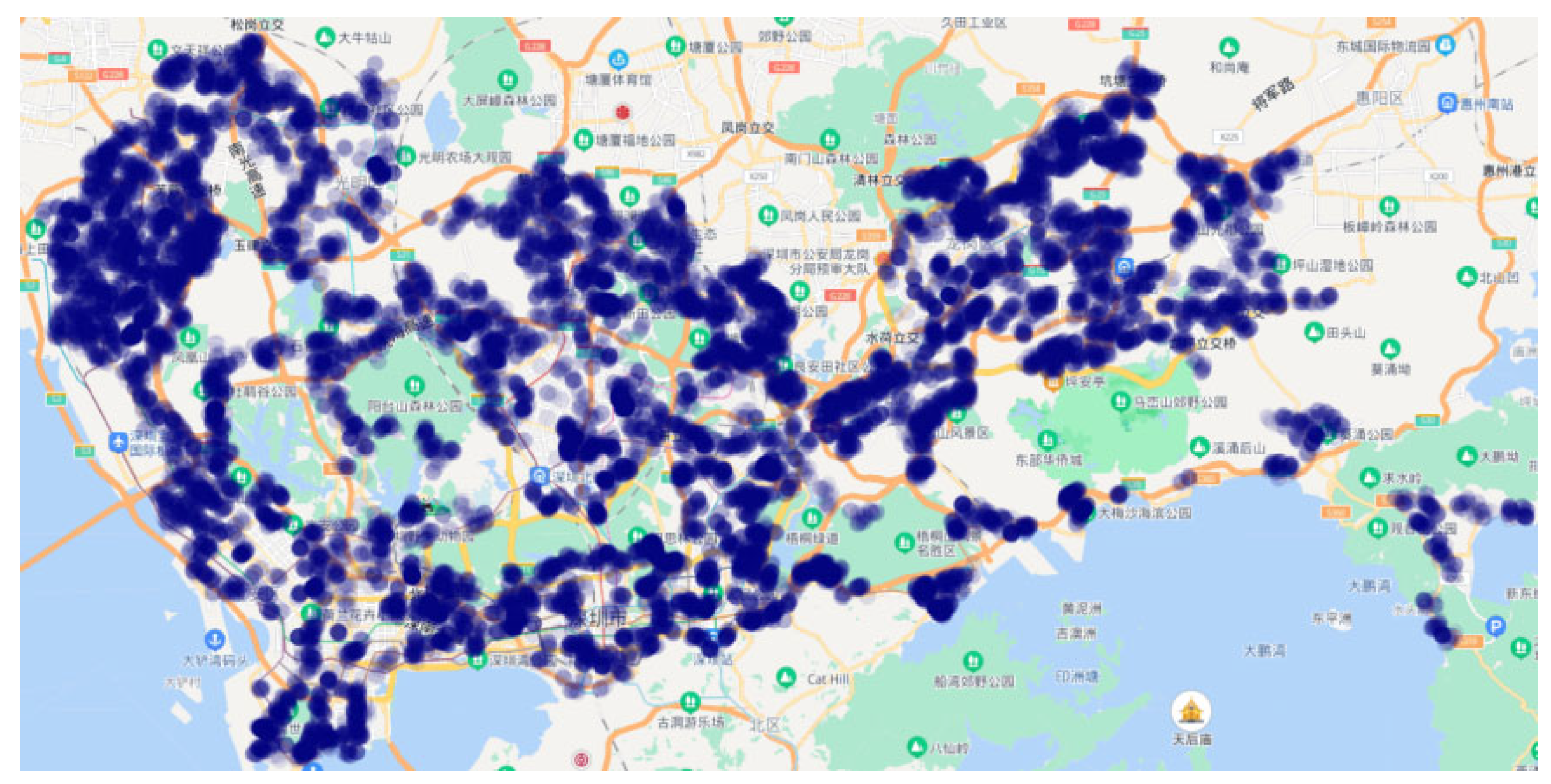
In this paper, the proposed model and method are validated and evaluated by taking Shenzhen city as an example. For the bus travel data, the data of the morning peak (7:00~9:00) trips in December 2020 were selected, with a daily average of 838,900 entries, accounting for 28.92% of the whole day trips. The average time distribution of passenger flow is shown in Figure 1, showing a trend of rising and then falling, with the peak located at around 8 o'clock; the average spatial distribution of passenger flow is shown in the heat map in Figure 2, with more concentrated passenger flow, mainly occurring in the city center. For station and line data, it specifically includes 5,500 bus station data, 1,020 bus line data, 234 subway station data and 11 subway line data. For residential POI data, the total number of residential POI data is 6,282, furthermore, the number of reachable communities for bus stations is 36,800, and the number of urban villages is 29,800.
3.7. Data Resources
3.7.1. Residential POI data crawling
(1) Website choosing
Compared with the mainstream real estate websites in China, "Housing World" and "Anjuke" have anti-crawler mechanism and need to complete the slider verification manually at regular intervals; "Chain Home" does not have anti-crawler mechanism. It is feasible to crawl data automatically and in bulk. Meanwhile, "Chain Home" covers 82 popular cities in China and has 230,000 pieces of residential data, which can meet the data demand.
(2) Crawling method
This paper adopts a breadth-first traversal crawling strategy and uses Python to build six sub-functional modules, including request configuration module, URL de-duplication module, robots protocol module, web crawling module, web parsing module and storage module, to crawl the residential POI data of "Chain Home" in a batch automatically under the premise of the standard operation process.
(3) Results
For Shenzhen, 4,574 communities and 1,708 urban villages were crawled. Among them, the communities are mainly distributed in the city center, with an average price of 62,400/ and a total of 5,361,900 people; the urban villages are more scattered, with an average price of 56,100/ and a total of 10,479,900 people. The total number of residential POI is compared with the resident population of 17,560,100 people in the Seventh Census Analysis Report, and the relative error is -9.79%, and the crawling result is basically in line with the reality. The specific distribution of subdivisions and urban villages is shown in Figure 3 and 4.
Figure 4.
Scatter Diagram of Urban Village Distribution.
3. 7.2. Bus and Subway Data Obtaining
(1) Platform choosing
Comparing with the domestic mainstream map open platform, the personal quota of Baidu data retrieval function is 30,000/day, while Tencent and Gaode are 10,000/day and 5,000/day respectively, therefore, this paper chooses Baidu map open platform to obtain bus and subway data.
(2) Obtaining method
In this paper, we use Python to write query statements conforming to the platform format, access the application programming interfaces of Baidu Map open platform, call the highly concurrent data retrieval function, and obtain the bus and subway data in Baidu Map automatically in batch.
(3) Results
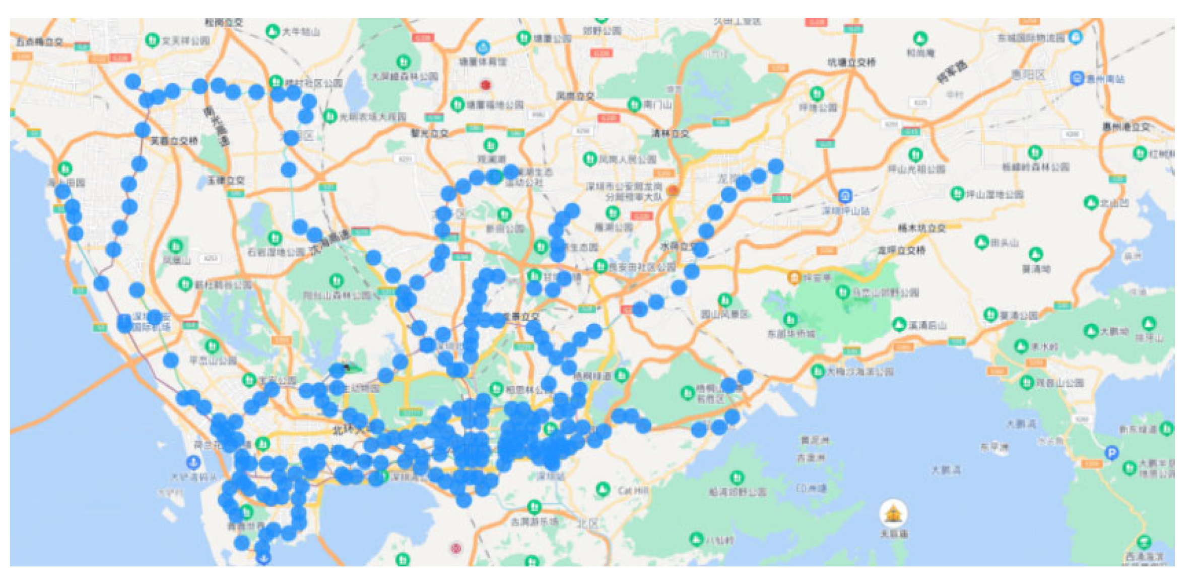
For Shenzhen, 1020 bus lines, 5050 bus stations, 11 metro lines and 234 metro stations were obtained. After comparing and checking with the data of Shenzhen Municipal Bureau of Transportation, the obtained data are relatively complete. The distribution maps of bus and subway stations are shown in Figure 5 and 4.
Figure 6.
Scatter Diagram of Subway Stations Distribution.
4. Results and Discussion
4.1. Regression Model Validation
4.1.1 Model Validity Analysis
Due to the lack of actual transit passenger residence data to compare with the projected transit passenger residence, this section focuses on verifying the accuracy of the total residential POI bus station ridership.
(1) Residential POI bus station ridership regression model
① Improved model
Based on equation (5), the modeling data were first divided into training set and test set, and the training set accounted for 80% of the data set, then the coefficients of the regression model were calculated by inputting the training set data, and finally the total number of passengers at residential POI bus stations were projected by inputting the test set data, and the mean absolute error (MAE), root mean square error (RMSE), and MAPE were calculated using the actual passenger flow at bus stations as the true value, respectively.
Original model
Based on equation (4), the accuracy of the original model is calculated by inputting the corresponding data and further compared with the results of the improved model.
(2) XGBoost-based residential POI bus station ridership projection model
In the same way as ①, after completing model tuning using the training set data, we input the test set data to impute the total number of passengers at residential POI bus stations and calculate MAE, RMSE and MAPE respectively.
The comparison results of the above models are shown in Table 2. The MAE, RMSE, and MAPE of the improved model of residential POI bus station ridership regression are the smallest and have the highest accuracy.
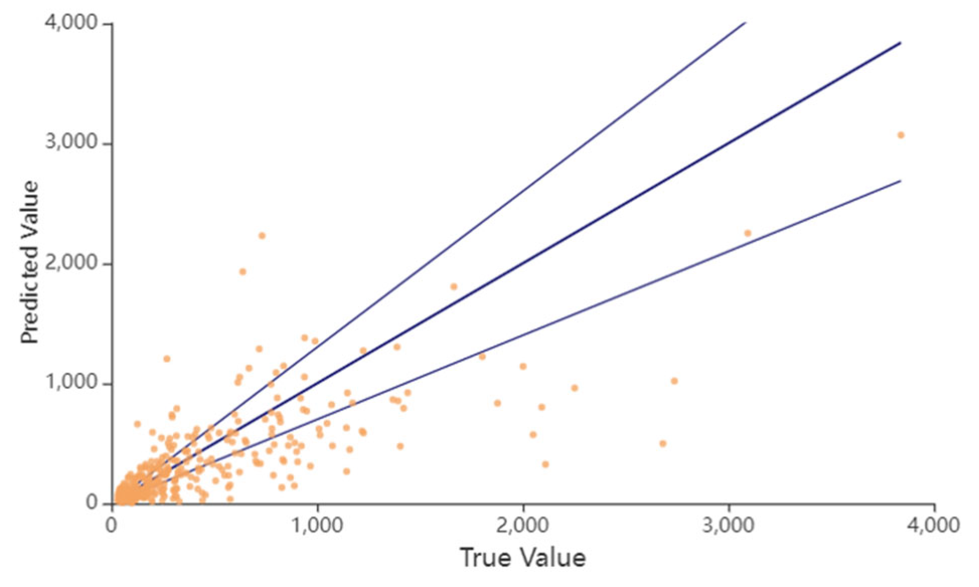
Further evaluating the optimal model, the comparison results between the predicted and true values of the training set and test set inputs are shown in Figure 7 and 8. The upper and lower lines in the figure indicate the error values of plus or minus 30% of the true values, and the more points falling within the error range indicate the higher accuracy of the model. It can be seen that the model prediction values are more concentrated and the results are reasonable. The percentage of the error of the results within 30% is 28.83% and 27.12% for the training set and test set, respectively, and the accuracy of the model is acceptable.
Figure 8.
Improved Regression Model of Residential POI Bus Station Passenger_ Test Set.
4.1.2. Reachable Distance Validation
The reachable distance is additionally divided into three categories of 300m, 700m and 1000m, and the corresponding data are input to calculate the model MAPE respectively, and the comparison results are shown in Figure 9. The results show that as the reachable distance increases, the model MAPE gradually increases and the model projection effect becomes worse. When the reachable distance is 500 m or more, the model effect changes more and is relatively worse, indicating that the maximum walking distance of bus passengers is within 500 m. Therefore, it is more reasonable to set 500 m as the reachable threshold in this paper.
4.2. Passenger Projection
4.2.1. Residency Projection
Based on the model coefficients in 5.2.3, the residential POI data are input to project the number of passengers from residential POI to each reachable bus station; further, to evaluate the accuracy of the projection, the total number of passengers at residential POI bus stations is verified. The specific values of residential POI to each reachable bus station ridership are shown in Table 6, and the results indicate that the number of urban village bus station ridership is greater than the number of community bus station ridership.
The MAE, RMSE, and MAPE of the total number of passengers at residential POI bus stations were calculated to be 155.490, 266.405, and 81.272%, respectively, using the actual passenger flow at the bus stations as the true value, and the results of the comparison between the predicted and true values are shown in Figure 10.
Using the number of passengers from residential POI to each reachable bus station as the weight, the actual number of passengers at the bus station is assigned to each residential POI, and the specific values of the actual number of passengers at the residential bus station are shown in Table 3. It can be seen that after the passenger flow allocation, the average value of the community is higher than before the allocation, and the average value of the urban village is lower than before the allocation, considering that the reason is that the number of passengers at the community bus station before the allocation is a larger ratio of the total number of passengers at the bus station, and the results are relatively reasonable.
Further, in order to evaluate the actual number of residential bus passengers at the place of residence, the calculation is based on the actual number of residential passengers at the bus station at the place of residence. The results show that the average actual number of residential bus passengers is 132.59, the average value of the community is 105.01 and the maximum value is 2769, and the average value of the urban village is 168.04 and the maximum value is 3602. The heat map of residential bus passengers distribution is shown in Figure 11, which shows that residential bus passengers is more distributed in downtown areas where public transit is more convenient. Compared with Figure 12 Residential POI number distribution heat map, observation shows that the number of residential POI in area ① and area ② is relatively close, but the number of residential bus passengers in area ② is much larger than that in area ①, considering the reason that area ① is located in the northwest of Baoan District, the residential POI is mainly in urban villages, and the willingness to travel by bus is weaker, while area ② is located in Longhua District, there are more subdivisions, and the willingness to travel by bus is stronger. The heat map of the residential bus passengers distribution with the reachability distance threshold set to 1000 m is further plotted, as shown in Figure 13 and compared with Figure 5-18, it is found that the projected residential bus passengers distribution does not vary significantly due to the change in the set reachability distance threshold, and the projected results are relatively reliable.
4.2.2. Trip ratio Projection
(1) Ratio of trips to bus stations in residential areas
Based on the residence projection results, the ratio of trips to bus stations in the residence is projected according to equation (7). Among them, the average value of the trip ratio of the community bus station is 0.0115 and the maximum value is 0.194; the average value of the trip ratio of the urban village bus station is 0.0073 and the maximum value is 0.187. To further verify the relationship between the number of bus station lines and the ratio of trips to bus stations in communities and urban villages, the ratio of trips to bus stations in communities and urban villages was divided into five intervals according to the quintile method, the mean values of the number of bus station routes in different zones were counted, as shown in Figure 14 and Figure 15.
(2) Ratio of trips by bus in residential areas
Based on the residence projection results, the ratio of trips by bus in residential areas is calculated according to equation (8). Statistically, the average ratio of trips by bus in residential areas is 0.0561, compared with the ratio of 0.0478 obtained by dividing the daily average of 838,900 morning peak transit trips by the resident population of 17,560,100 in Shenzhen, with an error of 17.61%, and the results are relatively reasonable. Among them, the average value of the community bus travel ratio is 0.0573 and the maximum value is 0.197; the average value of the urban village bus travel ratio is 0.0509 and the maximum value is 0.214. The frequency distribution of the ratio of bus trips in residential areas is shown in Figure 16, and the results show that the low ratio of bus trips is more common, which is consistent with the current situation of residents' travel; the frequency distribution of the ratio of bus trips in communities and urban villages is shown in Figure 17 and Figure 18, and overall, the ratio of bus trips in communities is higher than the ratio of bus trips in urban villages. The thermal distribution of the ratio of bus trips in communities and urban villages is shown in Figure 19 and Figure 20. It can be seen that the communities with a high ratio of bus trips are mainly concentrated in the city center, and the urban villages with a high ratio of bus trips are outside the city center and are more scattered.
Further, to verify the relationship between the community housing price, the number of reachable bus lines, the number of reachable subway lines and the average distance to reachable subway stations and the community transit travel ratio, the neighborhood transit travel ratio was divided into five intervals according to the quintile method, and the mean values of housing price, the number of reachable bus lines, the number of reachable subway lines and the average distance to reachable subway stations in different intervals were counted, as shown in Figure 21, Figure 22, Figure 23 and Figure 24. The results show that the ratio of community bus trips and the above factors all show a linear relationship, and the results determined by the functional relationship are consistent, the ratio of community bus trips is relatively reasonable.
5. Summary
In view of the current inconvenient and expensive data acquisition of bus passengers' residence, this paper takes into account the factors influencing the proportion of bus stop trips, and puts forward the idea of "calculating the residence of bus passengers from the characteristics of housing POI housing price, bus and station convenience". The regression model of residential POI bus station passenger number and the projection model of residential POI bus station passenger number based on XGBoost are constructed. Meanwhile, for the city of Shenzhen, the proposed model and method were verified and evaluated by using the bus travel data, residential POI data, and subway lines and stations data. The results show that the regression model has the highest accuracy, and the calculated results are consistent with the reality and relatively reasonable.
There are still some problems and inadequacies in this research. The following aspects are found to be further explored in the future:
(1) The reachable distance in this paper is simply set as a radius of 500 meters, which still has a certain deviation from the actual walking distance of passengers. In the future research, more accurate walking distance can be used, so as to better match the actual situation of passengers.
(2) For some websites with anti-crawler programs, it is impossible to crawl their data. As a result, there are still some errors between the residential POI data in this paper and the real situation. Therefore, the follow-up research can further study the principle of crawler, to update and supplement residential POI data in real time to make the data more accurate.
(3) The object of this study is mainly the residence of bus passengers in the morning rush hour. Subsequent studies can be combined with the bus travel data of other time periods, other types of POI data such as enterprise POI, entertainment POI, and other travel mode data such as by-subway and by-online-car, so as to expand the object of this study to the actual accurate OD projection of urban residents.
Author Contributions
Conceptualization, L.Z., L.X.Z., and Q.P.X.; methodology, L.Z. and L.X.Z.; software, Q.P.X.; validation, L.X.Z.; formal analysis, L.Z.; investigation, L.Z. and Q.P.X.; resources, L.Z.; data curation, L.X.Z. and Q.P.X.; writing—original draft preparation, L.X.Z. and Q.P.X.; writing—review and editing, L.Z. ; visualization, L.Z. and Q.P.X.; supervision, L. Z.; funding acquisition, L. Z.. All authors have read and agreed to the published version of the manuscript.
Funding
This work was supported by Shenzhen Science and Technology Plan Project (No.KJZD20230923115223047) and Shenzhen Higher Education Stable Support Plan Project(No.20231123103157001).
Data Availability Statement
The data used to support the findings of this study are available from the corresponding author upon request.
Conflicts of Interest
The authors declare that they have no conflicts of interest.
References
- Widyawan, Prakasa B., Putra D. W., et al. Big data Analytic for Estimation of Origin-Destination Matrix in Bus Rapid Transit System. 2017 3rd International Conference on Science and Technology - Computer (ICST), 2017, pp. 165-170.
- Takao R, Ikeuchi N, Suzuki H, et al. A Proposal for OD Data Estimation System of Bus Users with Intelligent Video Analysis and Its Application to Synerex. 2021 IEEE International Conference on Consumer Electronics (ICCE), 2021, pp. 1-4.
- Zhang W., S. , Lu M., Zhu J. J., et al. OD Calculation of bus passenger flow based on IC card and AVL data [J]. Computer Applications and Software: 2021-100.
- Liu B. K. The defect and prospect of existing OD survey method [J]. Shandong Jiaotong Keji, 2016 (01): 109-110.
- Jang, Y. , Ku D., Lee S. Pedestrian mode identification, classification and characterization by tracking mobile data[J]. Transportmetrica A: transport science, 2021: 1-29.
- Shiva, R. , Mehdi G., Hashemi S M, et al. A hybrid of Neuro-Fuzzy Inference System and Hidden Markov Model for Activity-Based Mobility Modeling of Cellphone Users. Computer Communications, Volume 173, 2021, Pages 79-94, ISSN 0140-3664.
- Sun Z, Liu J M, Yan N. Prediction of urban residents’ OD matrix based on mobile phone big data [J]. Mathematics in Practice and Theory, 2019, 49 (11): 68-77.
- Zhang X D, Jia L P, Deng S C, et al. Study on the operation characteristics of taxi and ride-hailing in Xiamen constrained by GPS track data and POI data [J]. Journal of Beijing University of Civil Engineering, 2021,37 (04): 60-68.
- Peng, F. , Song G. H., Zhu S. A method for extracting commuting trips of frequent passengers in urban public transportation [J]. Journal of Transportation Systems Engineerin, 2021, 21 (02): 158-165 + 172.
- Tang H T, Liu Y P, Wu Z C. Analysis of spatial heterogeneity of influencing factors of housing price based on POI data: a case study of Changsha[J]. Urban Problems, 2021 (02): 95-103.
- Wang Wei, John P. Attanucci, Nigel Wilson. Bus Passenger Origin-Destination Estimation and Related Analyses Using Automated Data Collection Systems. Journal of Public Transportation,2011,14 (4): 131-150.
- Catherine Vanderwaart, John P. Attanucci, Frederick P. Salvucci.Applications of Inferred Origins-Destinations and Interchanges in Bus Service Planning[J]. Transportation Research Record, 2017, 2652(1) : 70-77.
- Widyawan, B. Prakasa, D. W. Putra, S. S. Kusumawardani, B. T. Y. Widhiyanto, F. Habibie.Big Data Analytic for Estimation of Origin-Destination Matrix in Bus Rapid Transit System. 2017 3rd International Conference on Science and Technology - Computer (ICST), 2017, pp. 165-170.
- R.Takao, N. R.Takao, N. Ikeuchi, H. Suzuki, Y. Matsumoto. A Proposal for OD Data Estimation System of Bus Users with Intelligent Video Analysis and Its Application to Synerex. 2021 IEEE International Conference on Consumer Electronics (ICCE), 2021, pp. 1-4.
- Lan, C. Route-Level Transit Passenger Origin-Destination Trip Estimation from Automatic Passenger Counting Data: A Case Study in Edmonton[J]. 2015.
- Rodríguez González AB, Vinagre Díaz JJ, Wilby M R. Detailed Origin-Destination Matrices of Bus Passengers Using Radio Frequency Identification[J]. IEEE Intelligent Transportation Systems Magazine, 2022, 14(1).
- Ge Q, Fukuda D. Updating origin-destination matrices with aggregated data of GPS traces[J]. Transportation Research Part C: Emerging Technologies, 2016, 69:291-312.
- Zang H, Bolot J. Anonymization of Location Data Does not Work:A Large-scale Measurement Study[C]. The 17th Annual International Conference on Mobile Computing and Networking, Las Vegas, Nevada, USA,2011.
- Frias-Martinez V, Soguero C, Frias-Martinez E. Estimation of Urban Commuting Patterns Using Cellphone Network Data[C]. The ACM SIGKDD International Workshop on Urban Computing,Beijing, China, 2012.
- Shiva Rahimipou, Mehdi Ghatee, S.M. Hashemi, Ahmad Nickabadi. A hybrid of neuro-fuzzy inference system and hidden Markov Model for activity-based mobility modeling of cellphone users[J]. Computer Communications, Volume 173, 2021, Pages 79-94, ISSN 0140-3664.
- Jang, Y. , Ku D., Lee S. Pedestrian mode identification, classification and characterization by tracking mobile data[J]. Transportmetrica A: transport science, 2021: 1-29.
- Liu F., L. , Li N., Tian L. F., et al. Analysis and research on travel demand of public transport based on metropolitan comparison [J]. Highway,2020,65(10):230-237.
- Zhang X., M. , Gong D., Xie B. L., et al. A study of the effectiveness of epidemic prevention policies on public transit usage based on the theory of planned behaviors [J]. Journal of Transport Information and Safety,2021,39(06):117-125.
- Hu Y., Y. , Pu Z, Wang P. Study on the impacts of traffic carbon emission pricing on resident trip behavior using logit model [J]. Journal of Transportation Engineering and Information,2021,39(06):117-125.
- Liu Y., F. , An T., Qian Y. Z., et al. Exploring influence factors for travel mode choice in cities with different scales [J].China Journal of Highway and Transport,2022,35(04):286-297.
- Wang W., L. , Yu H. Research on evaluation method of pedestrian reachability and convenience of rail transit stations [J]. Tianjin Construction Science and Technology,2019,29(06):67-73.
- Zhang S., Y. , Yang Y., Chu Y. H., et al.Evaluation of Wuhan bus station satisfaction based on structural equation [J].Highways & Automotive Applications,2020(05):29-32+36.
- Cui N., N. , Gu H. Y., Shen T. Y.Study on the Impact of Transportation Spatial Layout on Urban Housing Prices — Based on the Correlation Analysis between Road Network Morphology and Housing Prices in Beijing[J].Price Theory and Practice, 2019(02):63-66.
- Kang, J. ,Luo J. J., Xue S Y, et al. An empirical study on the relationship between housing prices and residents’ income in Shanxi province [J]. Science & Technology Information,2022,20(12):129-132.
- Ren X., W. , Huang P. A Test of the mediating effect of population urbanization on house price [J].West Forum on Economy and Management,2021,32(03):58-66.
- Yu, X. , Wang M. Y., Dong X., et al.A study on migration tendency of floating population in urban villages: Taking the city of Xi’an as an Example [J]. Modern Urban Research,2021(08):10-16.
- Yao W., J. , Bai L. S. Implementation-oriented urban village traffic management optimization measures-Shenzhen city as an example [J].Traffic & Transportation,2021,34(S1):197-200.
- Hao Q., T. , Wang H. Y., Hao J. J. Study on influencing factors of community residents’ housing satisfaction-take Yijing community in Dazhou Sichuan province as an example [J]. Jiangxi Building Materials,2022(07):322-325+328.
- Liu Y., B. , Li X., Li A. X.Countermeasures for the treatment and promotion of traffic congestion and hidden dangers in "villages within city"-taking Buji Changlong Area of Shenzhen city as an example [J].Traffic & Transportation,2021,34(S1):201-205.
- Wang J., Q. , Zhan Y. T., Li S. J. Analysis of the relationship between traffic congestion and population density and car ownership in surrounding communities [J]. Auto Time,2020(09):32-33.
- Xia H., B. , Dai X. Y., Wang Y, et al. The analysis of traffic convenience on county level based on GIS [J]. Areal Research and Development,2006(03):120-124+130.
- Qi W., F. , Zhang J. J. Evaluation of Subway Station Convenience Based on Walking Living Circles — A Case Study of Hangzhou Metro Line 1[J].Architecture and Culture,2022(02):136-138.
- Xie G., W. , Qian L. B., Pang Y. Study on Public Transport Accessibility Measurement Based on GIS and Open Data[J].Logistics Technology,2021,44(12):102-106.
- Gan L., L. , Feng X. H., Bi J. L.,Jiang H. L. Study on Strength Prediction of High-Strength Concrete Based on Multivariate Nonlinear Regression Model[J].Concrete and Cement Products,2022(02):1-7.
- Abdul Joseph Fofanah,Ibrahim Kalokoh,Korjo Tesyon Hwase,Alex Peter Namagonya. Adaptive Neuro-Fuzzy Inference System with Non-Linear Regression Model for Online Learning Framework[J]. International Journal of Scientific and Engineering Research,2020,11(8).
- Wei M., Y. ,Li L. L.,Huang G., et al.Deep learning in EEG decoding: A review [J]. Chinese Journal of Biomedical Engineering,2019,38(04):464-472.
- Li L., M. , Hou M. M., Chen K. A Review of Research on the Interpretability of Deep Learning[J].Computer Applications, 2022,9:1-11.
Figure 1.
Time Distribution of Passenger Flow.
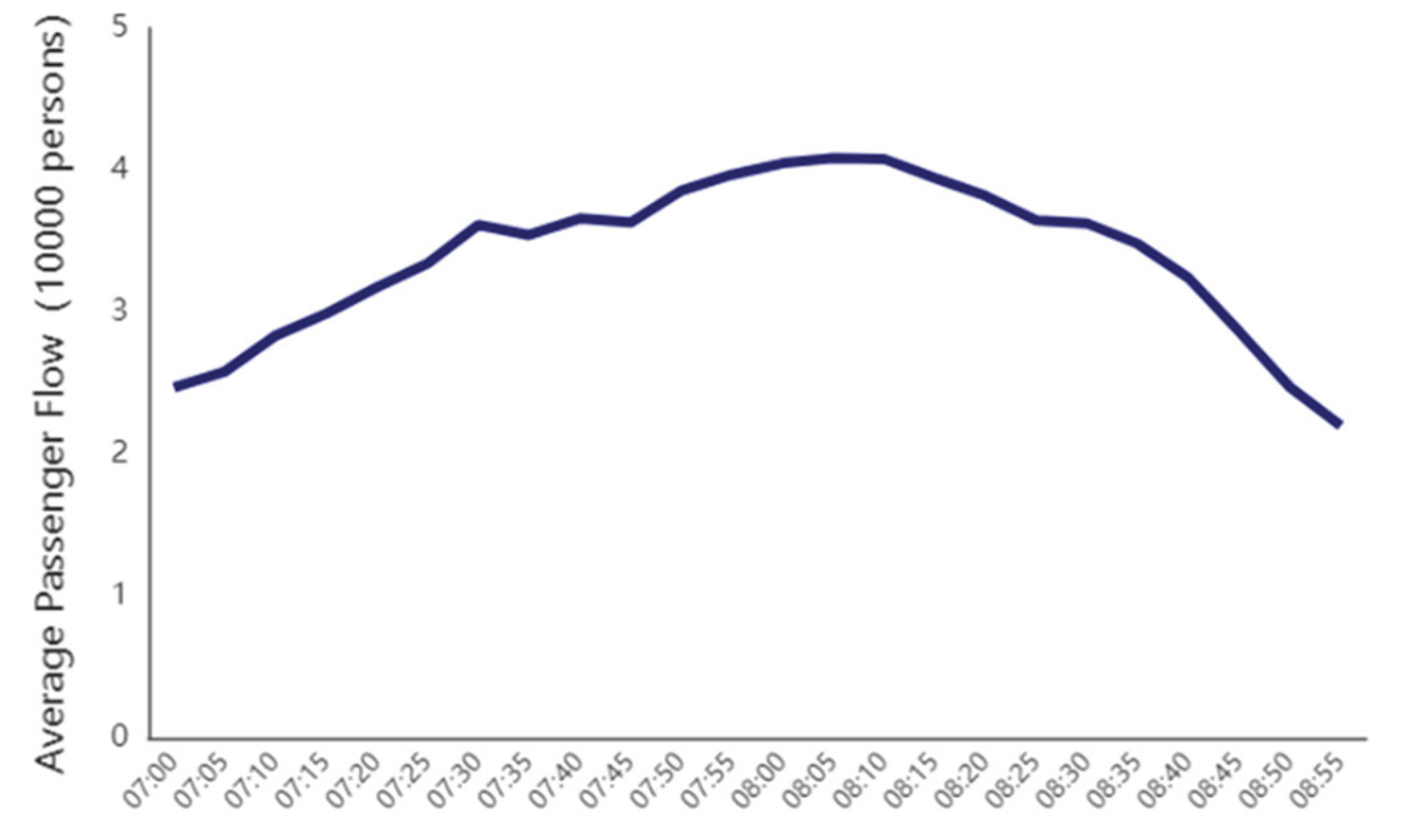
Figure 2.
Thermal Spatial Distribution Diagram of Passenger Flow.
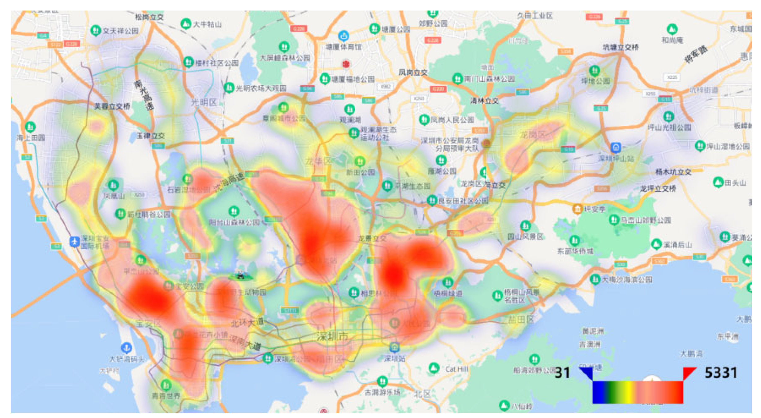
Figure 3.
Scatter Diagram of Community Distribution.
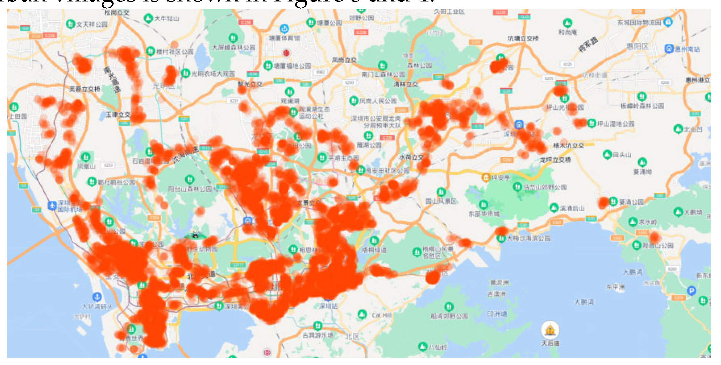
Figure 5.
Scatter Diagram of Bus Stations Distribution.
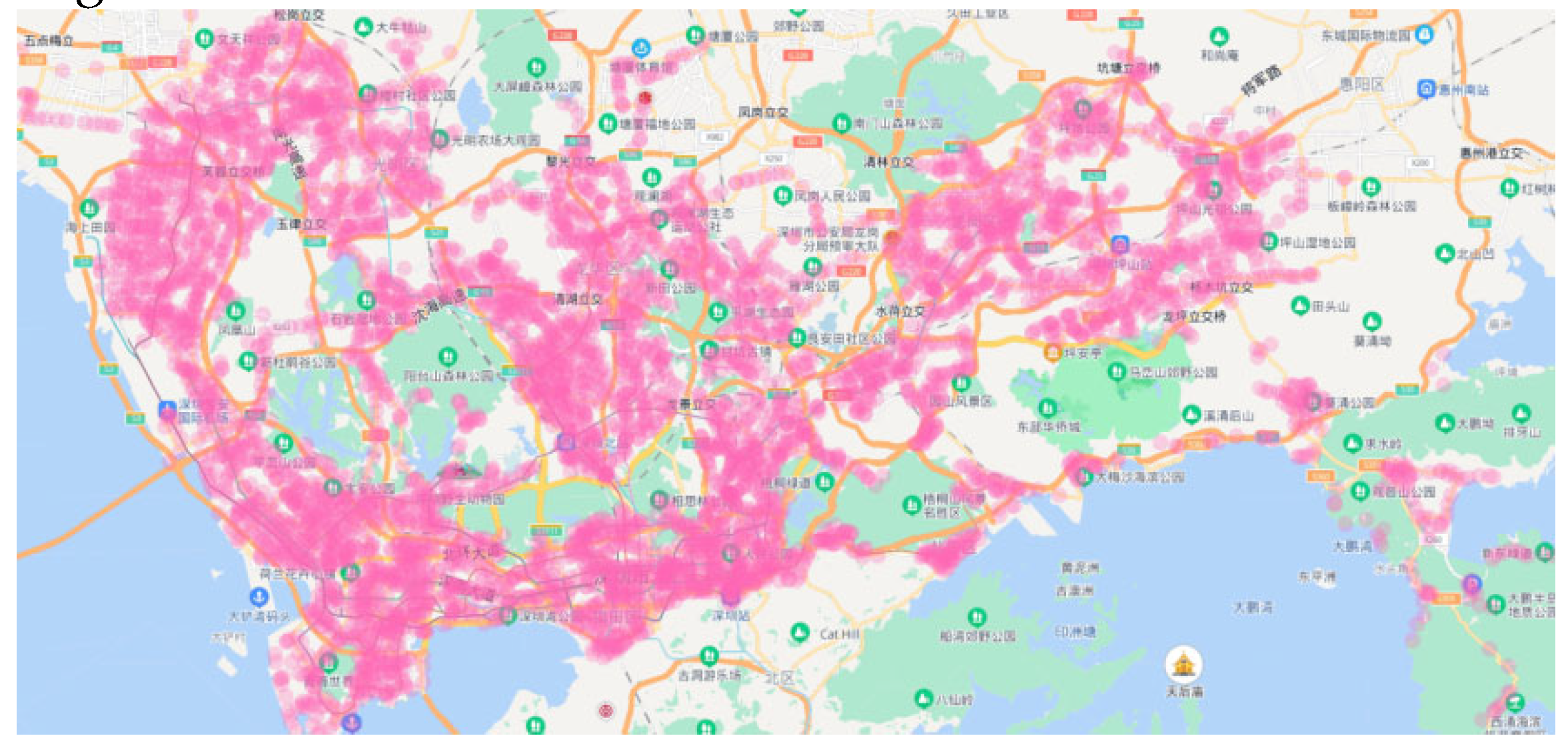
Figure 7.
Improved Regression Model of Residential POI Bus Station Passenger_ Training Set.
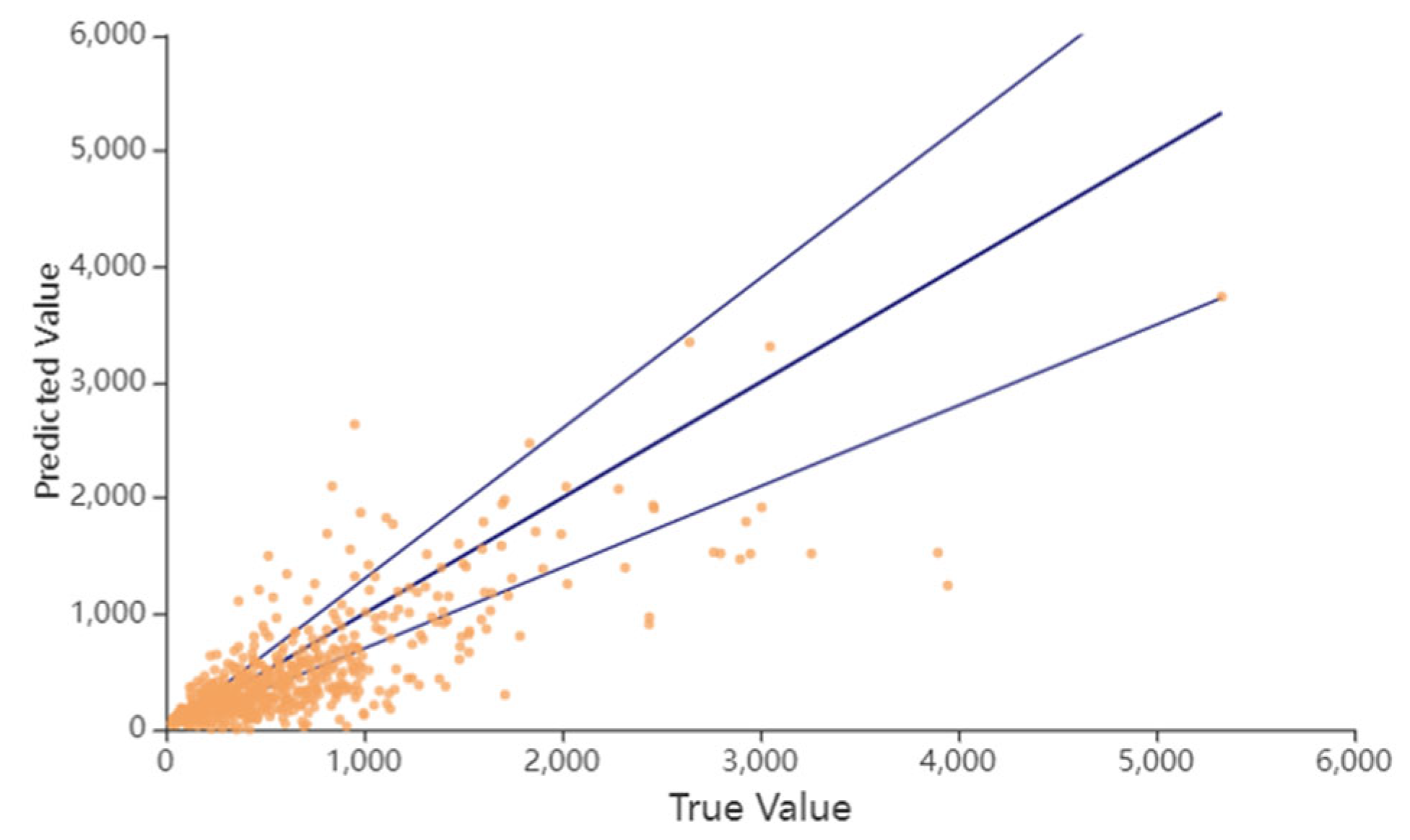
Figure 9.
MAPE Comparison of Different Reachable Walking Distance.
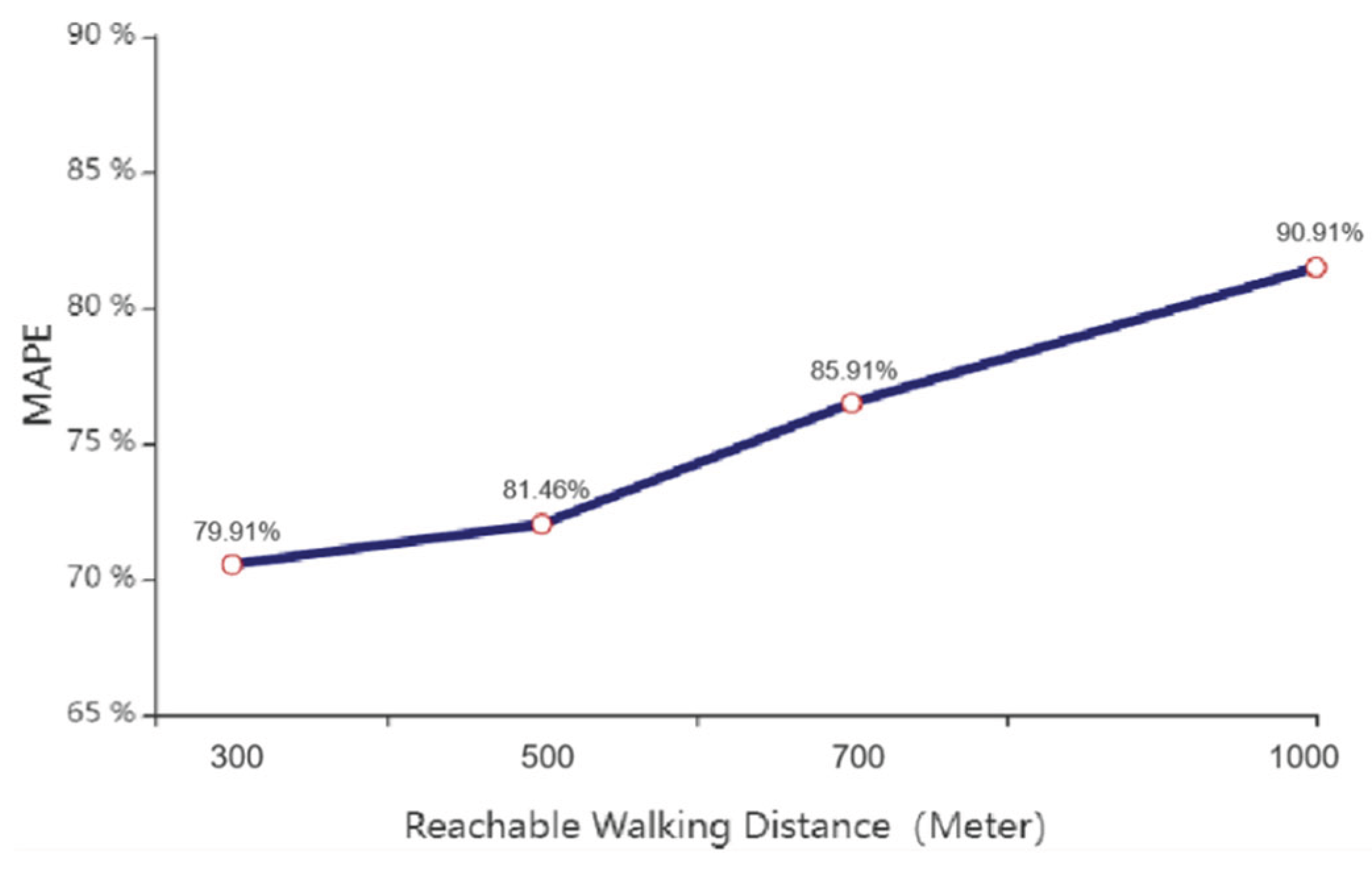
Figure 10.
Comparison between Residential POI Bus Station Total Passengers and Bus Station Actual Passenger Flow.
Figure 10.
Comparison between Residential POI Bus Station Total Passengers and Bus Station Actual Passenger Flow.
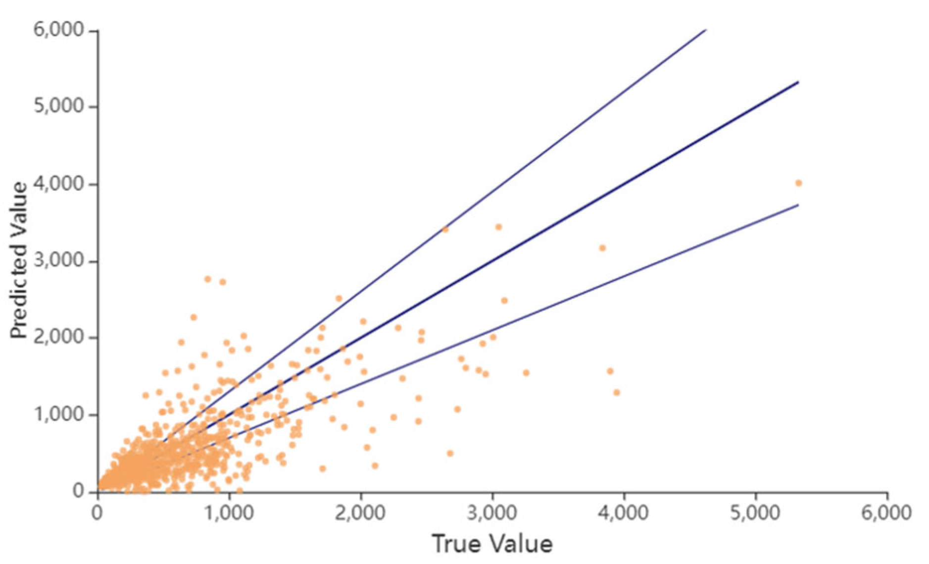
Figure 11.
Thermal Distribution Diagram of Bus Passenger Residence.
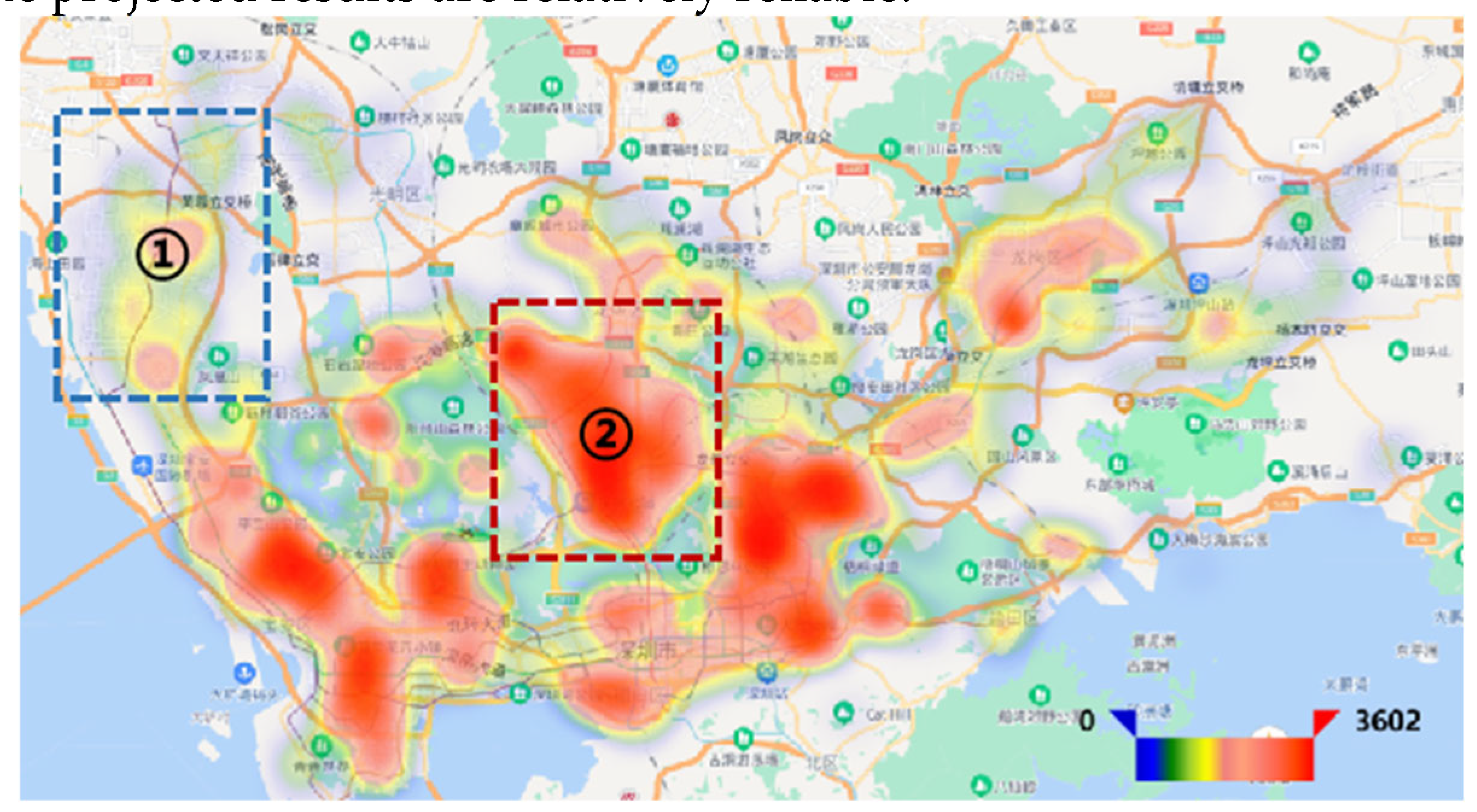
Figure 12.
Thermal Distribution Diagram of Residential POI Population.
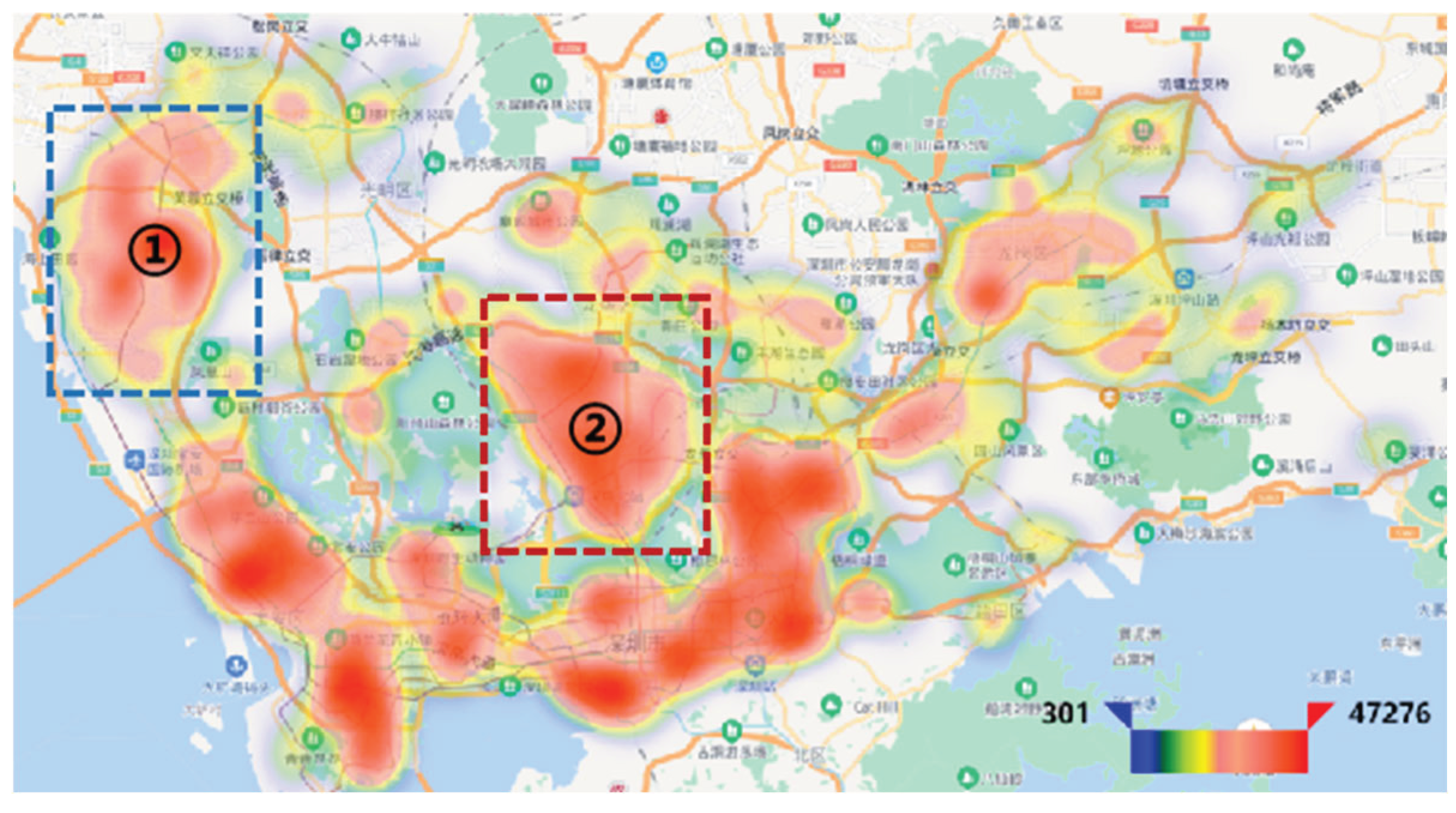
Figure 13.
Thermal Distribution Diagram of Bus Passenger Residence(1000M).
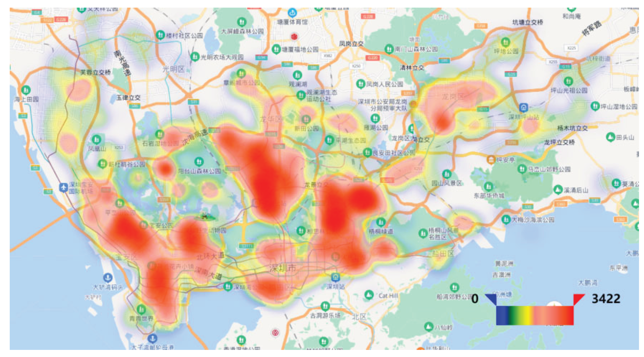
Figure 14.
Line Chart of Community Station Trip Ratio and Bus Station Lines.
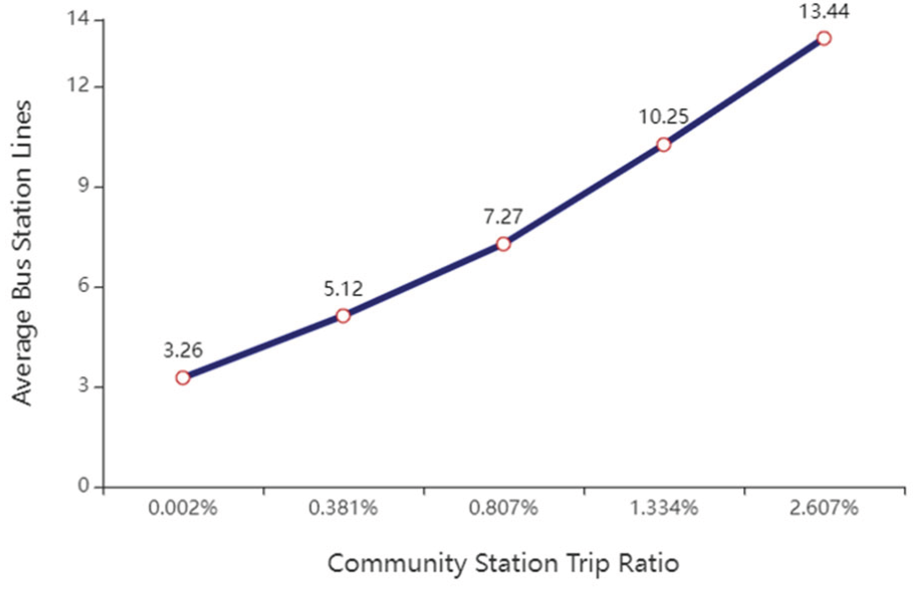
Figure 15.
Curving Diagram of Urban Village Station Trip Ratio and Bus Station Lines.
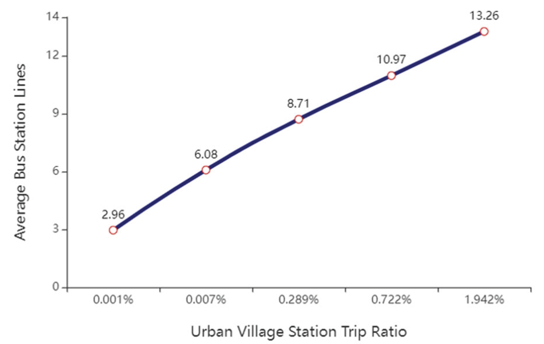
Figure 16.
Frequency Distribution of Residence Trip Ratio
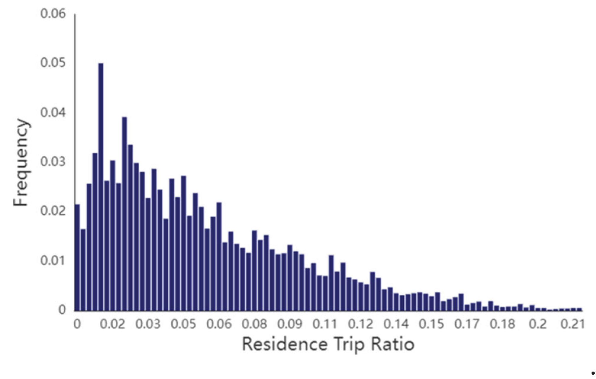
Figure 17.
Frequency Distribution of Community Trip Ratio.
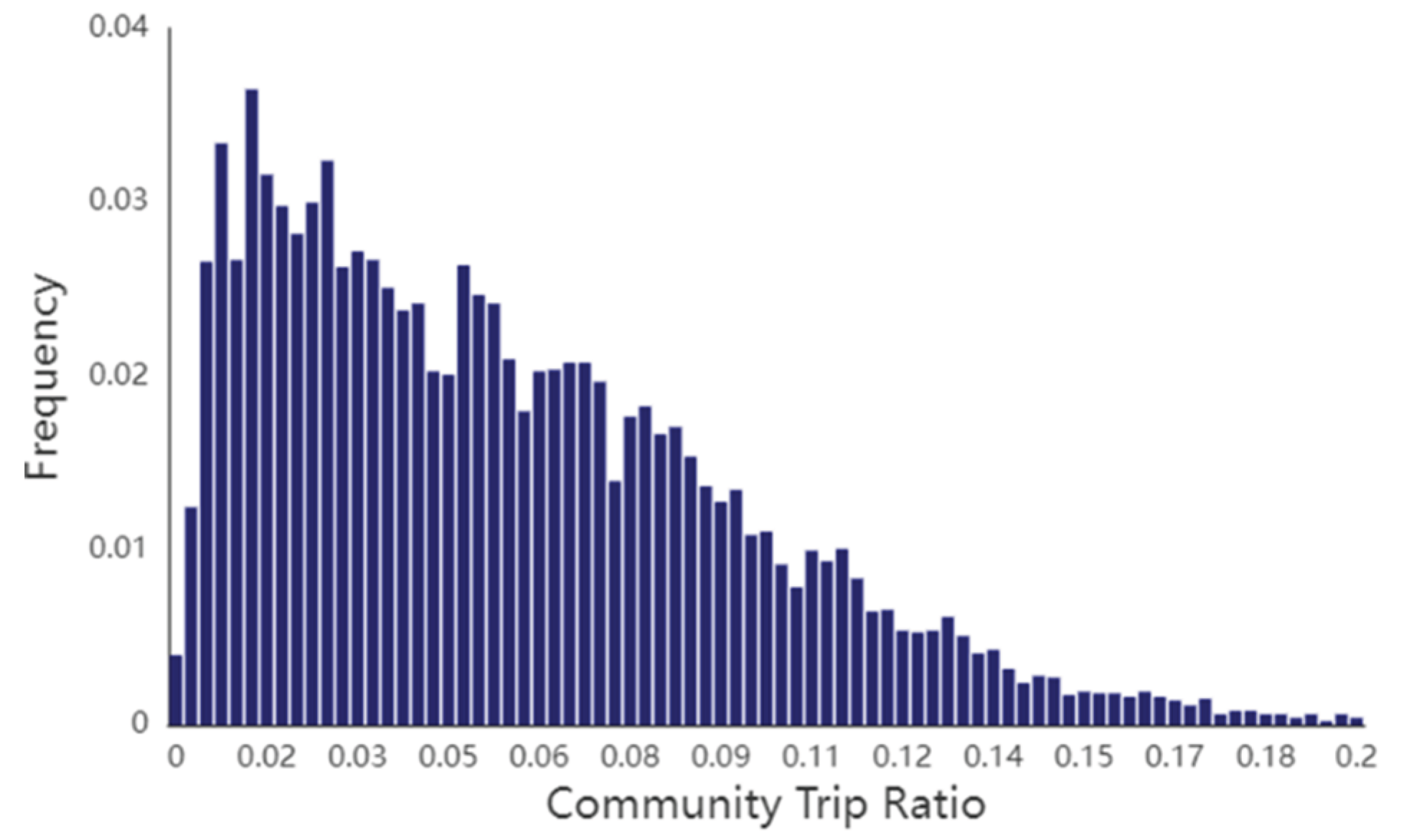
Figure 18.
Frequency Distribution of Urban Village Trip Ratio
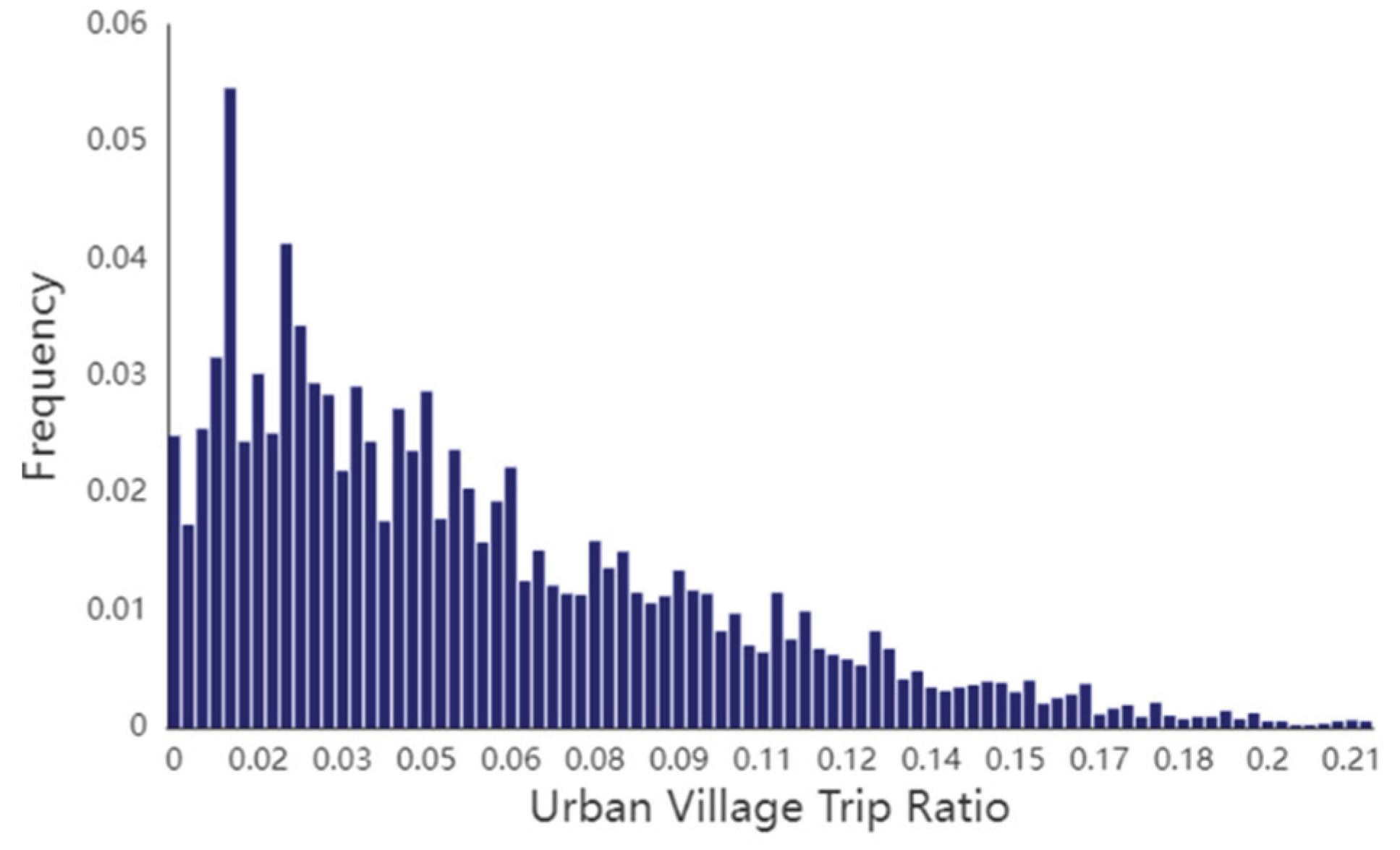
Figure 19.
Thermal Distribution Diagram of Community Trip Ratio
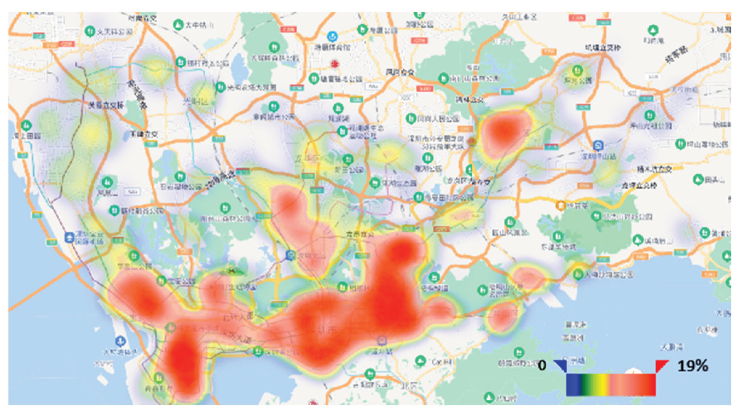
Figure 20.
Thermal Distribution Diagram of Urban Village Trip Ratio.
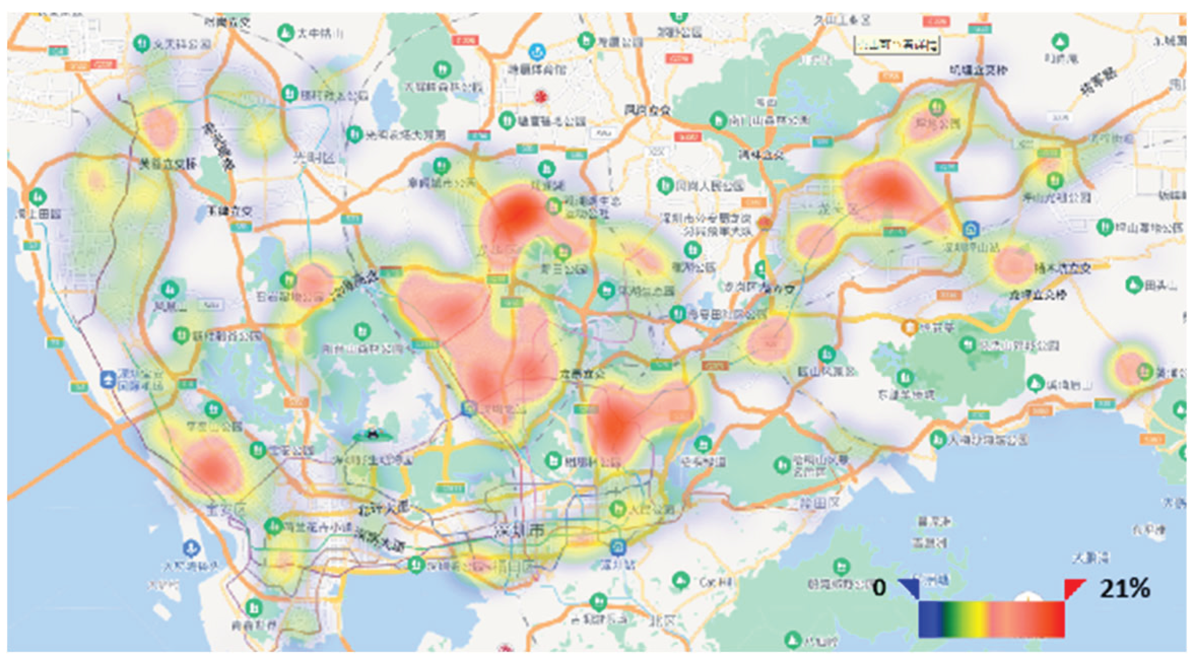
Figure 21.
Line Chart of Community Trip Ratio and House Price.
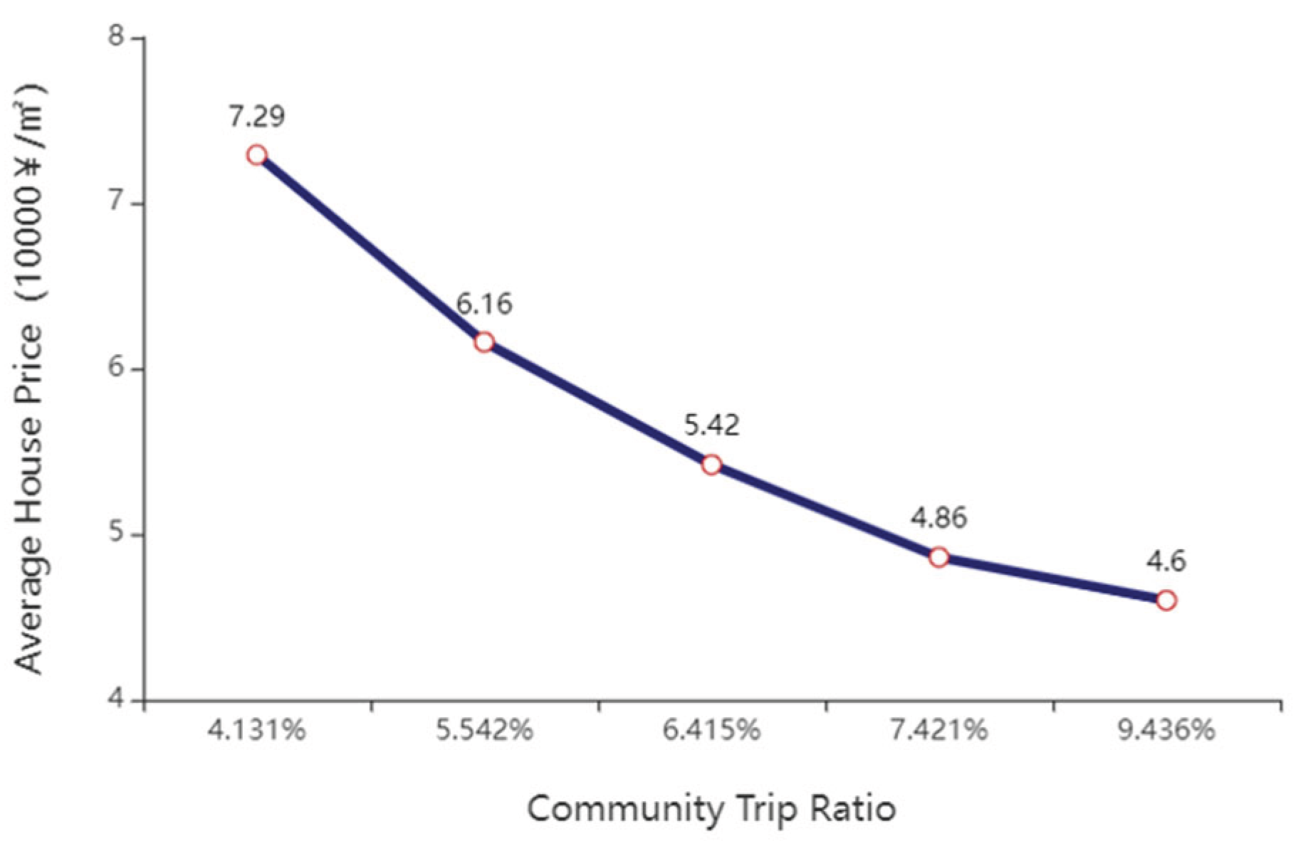
Figure 22.
Line Chart of Community Trip Ratio and Reachable Bus Lines.
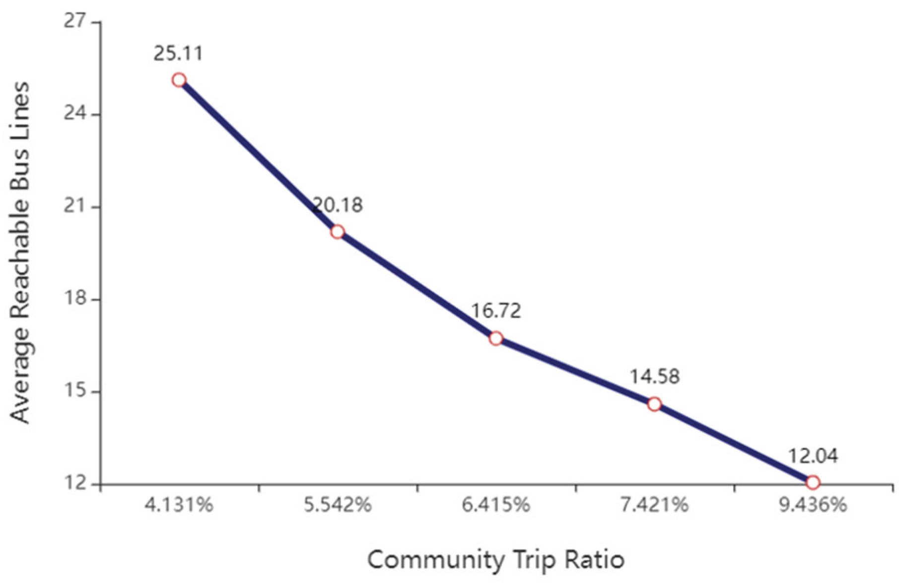
Figure 23.
Line Chart of Community Trip Ratio and Reachable Subway Lines.
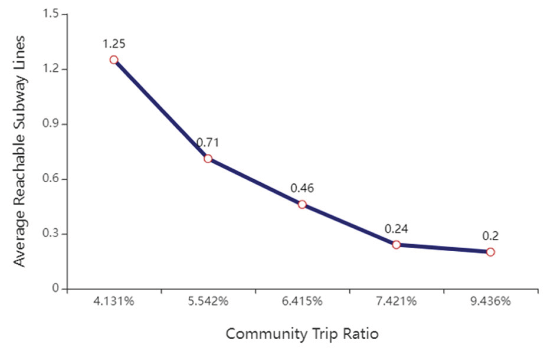
Figure 24.
Line Chart of Community Trip Ratio and Average Distance of Reachable Subway Station.
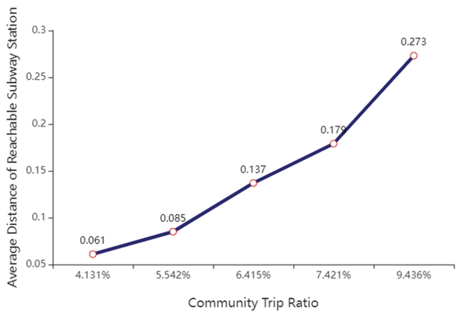

Table 1.
Indicators of Influencing Factors.
| Factor Categories | Influencing Factors | Indicators | Designing Way |
|---|---|---|---|
| Bus Travel Factors | Income per inhabitant in the place of residence | Residential POI Home Prices | Indirect |
| Age per inhabitant in the place of residence | Residential POI Type (community, urban village) |
Indirect | |
| Vehicle ownership per inhabitant in the place of residence | Indirect | ||
| Occupational share of residents in the place of residence | ———— | Excluded | |
| Convenience of bus in the place of residence | Number of residential POI reachable bus routes | Direct | |
| Number of residential POI reachable bus stations | |||
| Convenience of subway in the place of residence | Number of residential POI reachable subway lines | Direct | |
| Number of residential POI reachable subway stations average distance | |||
| Bus station Choosing Factors | Convenience of bus stations | Number of bus routes | Direct |
| Number of residential POI reachable bus stations distance |
Table 2.
Comparison of Models’ Accuracy.
| Model Results | MAE | RMSE | MAPE |
|---|---|---|---|
| Improved residential POI bus station ridership regression model | 161.027 | 288.069 | 72.024% |
| Original Residential POI bus station ridership regression model |
180.642 | 311.052 | 113.531% |
| XGBoost-based residential POI bus station ridership projection model | 167.124 | 295.868 | 82.472% |
Table 3.
Residential POI and Residence Bus Station Passenger.
| Type Values |
The number of passengers from residential POI to reachable bus stations | The actual number of passengers in residential bus station |
|---|---|---|
| Overall average | 21.48 | 23.07 |
| Community average | 19.34 | 22.29 |
| Urban villages average | 23.72 | 23.64 |
| Community maximum | 817 | 1327 |
| Urban villages maximum | 1088 | 1720 |
Disclaimer/Publisher’s Note: The statements, opinions and data contained in all publications are solely those of the individual author(s) and contributor(s) and not of MDPI and/or the editor(s). MDPI and/or the editor(s) disclaim responsibility for any injury to people or property resulting from any ideas, methods, instructions or products referred to in the content. |
© 2025 by the authors. Licensee MDPI, Basel, Switzerland. This article is an open access article distributed under the terms and conditions of the Creative Commons Attribution (CC BY) license (http://creativecommons.org/licenses/by/4.0/).
Copyright: This open access article is published under a Creative Commons CC BY 4.0 license, which permit the free download, distribution, and reuse, provided that the author and preprint are cited in any reuse.


