Submitted:
06 November 2025
Posted:
07 November 2025
You are already at the latest version
Abstract
This study presents numerical simulations of turbulent flow over a thick airfoil, modeled here as a semicircular cylinder, incorporating aerodynamic flow control (AFC) based on trapped vortex cells. Building upon previous work that focused on viscous effects, we now examine the influence of compressibility at various Mach numbers (M = 0.1, 0.2, and 0.3), corresponding to a diameterbased Reynolds number of 130, 000. The simulations employ a conventional RANS methodology, coupled with the Spalart-Allmaras and realizable k-ϵ turbulence models. To reinforce the validity of the results, cross-platform validation is performed using multiple numerical solvers, including pressure-based, density-based, and hybrid approaches (combining PISO/SIMPLE algorithms with the Kurganov-Noelle-Petrova scheme). Under the investigated conditions, the flow over the AFCintegrated configuration remains fully unseparated and exhibits outstanding lift performance. At Mach 0.2 (cruise conditions), the concept achieves a lift coefficient of approximately 6, about 95% of the theoretical maximum for a half-circular airfoil (2π), with a corresponding lift-to-drag ratio of around 24. As the Mach number increases to 0.3, the accelerated flow over the upper surface of the airfoil becomes locally transonic. Further analysis across a range of angles of attack (±150) at Mach 0.2 confirms the concept’s ability to maintain high lift and unseparated flow behavior, underscoring the effectiveness of the AFC system in enhancing aerodynamic performance.
Keywords:
thick airfoil
; aerodynamic flow control
; trapped vortex cells
; computational fluid dynamics
; separated flows
1. Introduction
Aerodynamic flow control (AFC) using Trapped Vortex Cells (TVC), strategically distributed across various surfaces of an obstacle, represents a promising alternative technology in the aerospace industry. By harnessing naturally occurring vortical structures and stabilizing them within engineered cavities, TVC systems enable enhanced lift generation, delayed flow separation, and improved overall aerodynamic efficiency – without relying on traditional moving parts or energy-intensive actuators. This semi-passive control approach offers significant potential for applications in aircraft design, unmanned aerial vehicles, and high-performance aerospace platforms, particularly where compactness, reliability, and energy savings are critical. Ongoing research continues to explore the scalability of TVC systems, their integration with advanced materials, and their performance under varying flow regimes, including compressible and transonic conditions.
A historical perspective on the AFC technology based on trapped vortex cell (TVC) is provided in the foundational works of Sedda et al. [1] and Lysenko et al. [2]. The concept of vortex trapping was first introduced by Ringleb [3], and later advanced by Kasper [4], who patented a glider design incorporating a trapped vortex structure to enhance lift. This innovation culminated in the first documented flight experiment using TVC technology – the tailless Kasper Bekas BKB-1 glider [5]. In the early 1990s, Savitsky et al. [6] expanded on these principles with the development and testing of the EKIP aircraft, a blended wing-body configuration equipped with multiple TVCs. Between 1995 and 2005, both experimental and numerical studies on thick airfoils (with chord thicknesses ranging from to ) confirmed the potential for achieving nearly unseparated flow, leading to enhanced aerodynamic performance and minimal energy losses from flow control systems [7].
Further systematic investigations were conducted on thick airfoils such as MQ1 CIRA and Göttingen (with chord thickness), integrated with TVCs. These efforts were part of the EU’s 6th Framework Programme (VortexCell2050) and research initiatives funded by the Russian Foundation for Basic Research (2005–2009). These studies deepened the understanding of vortex dynamics and flow control mechanisms, revealing critical Mach number thresholds where significant reorganization of flow structures within TVCs occurs – typically accompanied by increased drag and reduced lift. Comprehensive analyses of these phenomena are available in the works of Donelli et al. [8], Sedda et al. [1], Isaev [9], and Lysenko [2,10].
A novel bluff-body configuration featuring aerodynamic flow control (AFC) based on trapped vortex cells (TVCs) was recently introduced, supported by pioneering large-eddy simulations (LES) [2]. The design comprises a half-cylinder main body with diameter and span length D, complemented by two semi-spherical attachments. Despite a degree of abstraction in the AFC implementation, the system effectively maintained an almost fully unseparated flow over the obstacle. This configuration represents a preliminary concept, where the engine-driven air suction mechanism was emulated through boundary conditions imposing fixed negative mass flow rates. Aerodynamic performance, quantified by the lift-to-drag ratio (K), showed a marked improvement: the AFC-equipped bluff body achieved , in contrast to the baseline case without AFC, which exhibited negative lift and a ratio of . Energy losses attributed to the AFC system were estimated at approximately of the total drag force, indicating a favorable trade-off between control effort and aerodynamic gain. Figure 1 illustrates conceptual flow visualization using time-averaged streamlines over bluff bodies with and without AFC, respectively.
The next logical advancement in AFC technology was its integration into a fixed-wing configuration. For this purpose, a Clark Y airfoil was combined with a semicircular cylinder, serving as the fuselage, and outfitted with a system of three trapped vortex cells positioned on its upper surface. This concept is schematically illustrated in Figure 2,a. A numerical study was conducted using LES at baseline flow conditions: Mach number , Reynolds number and zero angle of attack. Figure 2 presents a schematic overview of the concept and its flow visualizations using the Q-criterion and line integral convolution (LIC) based on the time-averaged velocity field in the central vertical cross-section.
Despite demonstrating strong aerodynamic performance, with a lift-to-drag ratio of approximately , the simulations revealed several limitations of the AFC system. Specifically, additional losses were observed within the internal channels, along with the formation of secondary vortex structures inside the vortex cells (Figure 2,c). Another notable design feature identified during modeling was pronounced flow circulation near the lateral surfaces of the vortex cells, as shown in Figure 2,b. This effect is attributed to circulation interference caused by geometric discontinuities between the Clark Y airfoil and the semicircular fuselage. To mitigate these interactions in future designs, the addition of vertical ridges is recommended. This would suppress cross-flow along the aerodynamic surfaces and help maintain independent pressure distributions between the wing and fuselage.
Despite significant improvements in aerodynamic performance, the previously developed flow control system had not yet achieved fully unseparated flow. Building on this foundation, further advancements were made in the work by Lysenko [10], aiming to eliminate flow separation entirely. The bluff body was redesigned as a thick airfoil with a relative thickness of (equivalent to a semi-circular cylinder) and integrated with two trapped vortex cells. To streamline development and reduce interference from secondary vortex structures, the semi-spherical blocks used in earlier designs were removed. This simplification helped avoid complex interactions between unwanted eddies and the primary flow. Numerical simulations were conducted at a free-stream Reynolds number of , based on diameter, and a Mach number of , with a zero angle of attack.
From a numerical modeling standpoint, both Reynolds-averaged Navier-Stokes (RANS) and large-eddy-simulation (LES) approaches were employed by Lysenko [10]. Each method confirmed the presence of fully unseparated flow over the airfoil equipped with AFC, with aerodynamic coefficient discrepancies limited to approximately . Ultimately, the refined design achieved nearly complete unseparated flow, generating a lift force equivalent to roughly of the theoretical maximum value (), and delivering four times the lift-to-drag ratio of the original configuration [2]. Additionally, the influence of viscosity (Reynolds number effects) was examined. Results indicated that the aerodynamic characteristics of the improved concept were largely insensitive to viscosity variations. Across a broad Reynolds number range (), a modest increase in lift and aerodynamic efficiency was observed, with the drag coefficient remaining nearly constant and the performance trending linearly toward an asymptotic limit.
This study builds upon previous research [2,10] by numerically investigating the influence of compressibility by varying Mach numbers on the aerodynamic performance of the proposed concept. A series of numerical simulations are conducted using the classical RANS approach for Mach numbers , , and , with a fixed Reynolds number of . Additionally, the system’s behavior is evaluated across a range of angles of attack, .
The specific goals and objectives of the study are as follows:
- Perform flow simulations around the concept using RANS methodology at Mach numbers , , and , and zero angle of attack;
- Conduct cross-platform validation for the limiting case at , when the flow over airfoil’s upper surface becomes locally transonic, by comparing different numerical solvers for the compressible Navier-Stokes equations – specifically pressure-based, density-based, and hybrid approaches;
- Assess the impact of turbulence modeling by comparing Spalart-Allmaras (SA) and Realizable k- (RKE) models across the selected Mach number range; analyze the limiting case assuming the fluid inviscid.
- Highlight the significance of accurately specifying thermodynamic properties of air, such as viscosity, heat capacity, and thermal conductivity, and their influence on integral aerodynamic characteristics;
- Analyze the aerodynamic performance of the system at various angles of attack within the range of ;
- Ultimately, the study revealed that the aerodynamic performance of the system remains largely unaffected by Mach numbers up to , consistently maintaining the fully unseparated flow. Under cruise conditions at , this behavior is associated with a high lift coefficient of , which corresponds to approximately of the theoretical maximum value of . The resulting lift-to-drag ratio is around 24.
The article is presented in five parts. The first two sections are devoted to the problem statement and aspects of numerical and mathematical modeling. Then the main results are presented. The fifth part provides a brief discussion and critical review. At the end, the main conclusions are drawn.
2. Problem Statement and Theoretical Considerations
In this section a brief problem statement and key design features of the aerodynamic flow control system are presented. A brief mathematical background of the Reynolds-averaged Navier-Stokes approach accompanied by the Spalart-Allmaras and k- realizable turbulence models are discussed as well.
The turbulent flow is characterized by the following Reynolds and Mach numbers: and , respectively. Here is the density, U is the far-field velocity, a is the speed of sound, represents the dynamic molecular viscosity, D is the diameter of the thick airfoil (semi-circular cylinder). The subscript ∞ indicates the flow parameters at the inlet boundary. The drag and lift coefficients are defined as and , where and are forces acting in the stream-wise and vertical directions. The pressure coefficient is specified as , where p being the static pressure. All numerical simulations were performed at the fixed Reynolds number, , and the following Mach numbers, , , and .
2.1. Overview of the Aerodynamic Flow Control Concept Based on the Trapped Vortex Cells
The primary design dimensions of the thick airfoil, both with and without an aerodynamic flow control system, are depicted in Figure 3. A bluff-body (BB hereafter) is composed of a main block shaped as a half-cylinder with a diameter D and a span length of D. The diameter of the half-cylinder, D, serves as the linear reference scale. The overall width, height, and span lengths of the bluff body are , , and , respectively. BB with aerodynamic flow control incorporates a system of the two trapped vortex cells, with diameters of and respectively, positioned on its suction (upper) side. Each TVC has a span length equal to D. Two vortex cells are connected by an arch-shaped channel. The outlet section of the channel, with a surface area of , is used for air suction (Figure 4,a).
The present concept has been redesigned compared to initial study [2], resulting in nearly unseparated flow past the airfoil. It is important to highlight that this system was developed after several dozen optimization iterations. This concept also abstracts the aerodynamic flow control system for air suction by imposing a fixed pressure drop assuming a passive method is employed. As initially reported by Lysenko [10], a pressure drop of Pa was sufficient to sustain fully unseparated flow over a thick airfoil at a low Mach number of . However, as the free-stream velocity increases toward Mach , a greater static pressure drop, up to Pa, is required to maintain similar flow behavior. In the current model, the consumed air is withdrawn inside BB, which is not a realistic scenario for real-life applications. However, in a broader context, aircraft dynamics require a feedback control loop in which air suction forcing is dynamically adjusted to achieve optimal system performance. In this context, the present flow control method can be regarded as active. Preliminary studies indicate that increasing the forcing up to allows the flow over the obstacle to remain unseparated while preserving similar large-scale vortex structures in the TVCs. However, this is accompanied by penalties in the form of increased drag force. While further detailed studies are necessary to model realistic air suction using an aircraft engine system, the authors believe that this design serves as a satisfactory proof-of-concept and holds significant potential for further development.
The physics and topology of the flow over BB without trapped vortex cells are qualitatively similar to the flow over a semi-circular cylinder at , as discussed in detail previously [11]. At a Reynolds number of , the separation of the laminar boundary layers occurs in the sub-critical flow regime. This condition results in complex, nonlinear interactions between near and far wakes characterized by two types of flow instabilities (Figure 4, b). The Kelvin-Helmholtz instability of the separated shear layer, along with vortex shedding (Bénard/von Kármán instability), dominates the wake. Figure 4, c shows the schematic flow over the BB with integrated vortex cells. Unlike the initial study [2], this design completely rearranges the flow over the airfoil, making it predominantly unseparated.
To avoid any confusion, all numerical simulations presented in this work were conducted in two-dimensional () space.
2.2. Basic Governing Equations
In this subsection the governing equations for the turbulent compressible flows for the Reynolds-averaged simulations are presented. The Cartesian tensor notation, where t and are independent variables representing time and spatial coordinates of a Cartesian coordinate system , is used. The three components of the velocity vector are denoted (). The summation convection over repeated indices applies unless otherwise is noted.
The Favre-averaged (i.e. mass-density weighted) equations for mass, momentum, and energy for the turbulent compressible flows are:
Here, the overbar denotes Reynolds averaging, while the tilde denotes Favre averaging: denotes the density, is the velocity, p is the pressure, is the enthalpy, T is the temperature, is the heat capacity and is the thermal diffusivity.
Here, is calculated as a function of temperature from a set of coefficients taken from NIST-JANAF thermochemical tables [12] or technical report NASA/TP-2002-211556 [13]. The thermal diffusivity is modeled as
where is the molecular viscosity (calculated according to the Sutherland’s law), R is the gas constant, represents heat capacity at constant volume. is the specific heat averaged over the temperature interval from the reference temperature to the actual mean temperature, , where and . It worth noting when equation of state is resented by the ideal gas law, the alternative method based on the kinetic theory can be applied to compute air thermodynamic properties (i.e., viscosity, thermal conductivity and specific heat).
The turbulence flux is derived according to the gradient hypothesis
where is the turbulence viscosity and is a turbulence Prandtl number (here ).
The stress tensor for a Newtonian fluid is expressed as
The Reynolds stresses are modeled according to
2.3. The Spalart-Allmaras Turbulence Model
The Spalart-Allmaras turbulence model [14] (SA here and after) solves a modeled transport equation for the kinematic eddy (turbulent) viscosity () as
where and are production and destruction of the turbulence viscosity that occurs in the near-wall region due to wall blocking and viscous damping, respectively. and are the constants.
The turbulent viscosity, , is computed as follows:
where , – constant and is the kinematic molecular viscosity.
The production term, , is modeled as
where d is the distance from the wall, and are the constants and is a scalar to measure of the deformation tensor. In the present study, is computed according to the modification proposed by Dacles-Mariani et al. [16] to combine both vorticity and the strain tensors:
where
The destruction term, is modeled as
Here, , , are model constants.
2.4. The Realizable k- Turbulence Model
The realizable k- turbulence model of Shih [15] (RKE here and after) is based on the turbulence kinetic energy () and its dissipation rate (), where the turbulence viscosity is defined as
The modeled transport equations are:
where
Here, G represents production of the turbulence kinetic energy due to the mean velocity gradients, is contribution of the fluctuating dilatation in compressible turbulence, is a constant and and are the turbulence Prandtl numbers for and , respectively.
The production of the turbulence kinetic energy is modeled as
The coefficient required to compute the turbulence viscosity in Eq. 5 is no longer constant and defined as the following equation:
Under some assumptions the term can be computed as the mean rate-of-rotation tensor viewed in a moving reference frame with the angular velocity , . The model constants are and , where
Effects of compressibility for high-Mach-number flows in the k- model is accounted by including the dilatation dissipation term , which is modeled according to proposal by Sarkar [17]:
where represents the turbulent Mach number and a is the speed of sound.
2.5. Basic Governing Equations in Conservative Form
Sometimes, it is useful to provide the governing equations in the conservation form:
where is the vector of conservative variables, and are the convective and viscous fluxes vectors, respectively:
Here, the stare equations are defined as follow: represents the total energy per unit mass, is the internal energy per unit mass, is the total enthalpy, R is the gas constant, is the specific heat ratio, is the viscous stress tensor and is the heat flux vector.
3. Brief Aspects of Numerical Simulations
This section provides a concise overview of the numerical method, along with descriptions of the computational domain, grids, boundary and initial conditions.
3.1. Overview of the Numerical Methodology
Several numerical approaches to solve the Favre-averaged Navier-Stokes (RANS) equations are used in the present study. Two of them are so-called pressure- and density-based solvers implemented in the CFD platform Ansys Fluent 2021R1 [18] (hereinafter, AF). And an alternative so-called hybrid solver implemented in the open-source OpenFOAM [19] (hereinafter, OF) framework. The term ’solver’ here refers to a generalized numerical method used to solve the fluid dynamics equations.
- Pressure-based approach belongs to a general class of methods called the projection method [20,21], where the continuity of the velocity filed is achieved by solving pressure-correction equation. The pressure-based solver is implemented as a finite volume method (FVM) utilizing a second-order upwind scheme (SOU) for all convective terms and an implicit Euler method (bounded BDF-2) for time integration [22]. The time integration step is chosen to ensure that the local Courant number is less than ten, . The so-called pressure-based coupled algorithm is used, which solves a coupled systems of equations comprising the momentum and pressure-based continuity equations. The system of linear algebraic equations is solved using the algebraic multigrid method (AMG) accompanied by the additive correction strategy [23] and the classical iterative Gauss-Seidel procedure.
- Density-based approach is a Godunov-type FVM solver. In his classical paper of 1959, Godunov [24] presented a conservative extension of the first–order upwind scheme to non-linear systems of hyperbolic conservation laws. The key ingredient of the scheme is the solution of the Riemann problem [25], which is approximated by the advection upstream splitting method (AUSM) [26] in the present study. Other numerical aspects like time integration, discretization schemes and linear solvers were set up in the same spirit as for the pressure-based approach.
- Hybrid approach is alternative method to integrate the mass, momentum and energy conservative equations by coupling the PIMPLE (combination of PISO/SIMPLE) algorithm [27] with a corresponding Kurganov-Noelle-Petrova scheme (KNP) [28] for non-oscillating discretization of the convective and diffusive terms. The hybrid method based on the coupled PIMPLE algorithm and KNP scheme meets the requirements on monotonicity and allows to simulate turbulent flows in a wide range of a Mach number, . The hybrid approach was implemented as a so-called `pimpleCentralFoam’ solver based on FVM supported by the OpenFOAM platform [19] with specific details provided by Krpaposhin et al. [29]. A stabilized preconditioned (bi)-conjugate gradients method (PBiCGStab) accompanied by the diagonal incomplete-LU preconditioner was used to solve the linear systems of the algebraic equations with the absolute tolerance of . A limited advection scheme, so called `vanLeer’ [30], which belong to a family of TVD schemes, was utilized to approximate convective and diffusive fluxes computed by KNP. Integration in time was handled by the first-order implicit Euler method with a restriction of .
3.2. Computational Grids
The planar, unstructured, hexahedral-dominated baseline grid (designated as A0) was constructed as follows. The computational domain was defined as a rectangular block with dimensions , initially seeded with nodes along the x and y directions. To enhance resolution, the region spanning to was adapted using a refinement coefficient. Within this, the central block from to was further refined to a uniform cell size of . At the core of the domain, a cylindrical region with a radius of , centered at the origin of the Cartesian coordinate system, was meshed with a fine uniform cell size of . A viscous sub-grid was applied around the obstacle, featuring an average wall-normal spacing of , an expansion factor of , and a total of five layers. For the second grid (referred to as A1), the cylindrical region of radius was re-meshed with an even finer uniform cell size of . The finest grid (referred to as A2) was then generated by adapting the cylindrical region of the A1 grid using an additional refinement. Details of the A0 and A3 grids are illustrated in Figure 5.
3.3. A Near-Wall Modeling Treatment
A wall treatment combining a two-layer model with enhanced wall functions is used for the realizable k- turbulence model [18]. This method maintains the accuracy of the standard two-layer approach for fine near-wall meshes while minimizing accuracy loss for wall-function meshes. The two-layer approach assumes that the computational domain is divided into viscosity-affected and fully turbulent regions. The demarcation is determined by a wall-distance-based turbulent Reynolds number, with the wall-normal distance, y, calculated at the cell centers. In the fully turbulent region (>200), the standard RKE model is utilized. In the viscosity-affected near-wall region, the one-equation model by Wolfshtein [31] is applied, where the computation of turbulent viscosity is modified by introducing a length scale parameter proposed by Chen and Patel [32]. Finally, the blending between the two regions is computed using the method proposed by Jongen [33].
The Spalart-Allmaras turbulence model implemented in AF has been extended with a - insensitive wall treatment, which allows to apply model independent of the near-wall resolution and blends automatically from a viscous sublayer formulation to a logarithmic formulation [18]. At the same time on the intermediate grids, , its continues to handle integrity and provides consistent wall shear stresses. For the hybrid solver implemented in OF, the SA turbulence model was used accompanied by the `nutUBlendedWallFunction’ boundary condition, which provides a wall constraint on the turbulent viscosity, i.e. , based on velocity. In this case a binomial-type wall-function blending method was applied to approximate between the viscous and inertial sublayers [34].
3.4. Boundary and Initial Conditions
Boundary conditions were defined to ensure that the free-stream parameters matched the target Reynolds and Mach numbers, set at and , respectively. Table 1 outlines the free-stream values used to determine the Mach number at the inlet boundary, adjusted according to bluff body altitude to reflect atmospheric variations with elevation above sea level (h). Notably, the Reynolds number remained constant across all Mach number cases. Compressibility effects were modeled using the ideal gas law. Thermodynamic properties like dynamic viscosity, thermal conductivity, and heat capacity were computed either via kinetic gas theory or temperature-dependent polynomial functions. Free-stream turbulence was characterized by a turbulence intensity of and a hydraulic diameter equal to D. At the inlet boundary, fixed values were assigned for free-stream velocity and total temperature, while a fixed static pressure was imposed at the outlet. The body surface was treated as adiabatic with no-slip wall conditions. Air suction from the vortex cell system was simulated by applying a static pressure drop ranging from to Pa, depending on the Mach number. The initial conditions corresponded to a sudden stop of the body in the fluid flow, meaning the inlet boundary conditions were initially extended to the entire computational domain.
3.5. Critical Remark on RANS Methodology Validation and Verification
It is worth noting that the development of the AFC technology in previous studies [2,10] primarily focused on large-eddy simulation (LES), with the classical RANS approach serving as a supplementary tool. A parallel objective was the rigorous evaluation of the numerical platform’s capability to predict turbulent separated flows, encompassing both internal and external aerodynamic configurations. To support this effort, the subgrid-scale incompressibility assumption was frequently employed, restricting free-stream Mach numbers to . The Reynolds number was similarly constrained to , under the assumption that the boundary layer along bluff body walls remains laminar. Key reference cases for AFC development included flow studies over semicircular [11] and circular [35] cylinders, conducted at and , respectively. These cases provided foundational insights into AFC performance under the above flow conditions.
As an initial step in further investigating the Mach-number dependence of the AFC technology, this paper focuses on the application of the RANS methodology. It is important to note that over the past two decades, extensive research has been performed to validate and verify the RANS approach in the context of turbulent separated flows. Several fundamental studies addressing critical components of the evolving AFC framework are particularly noteworthy:
- Isaev et al. [36,37] examined the lid-driven cavity flow using an incompressible formulation. The analogy to trapped vortex cells (TVCs) is evident, as the primary vortex core can be considered inviscid with constant vorticity, closely linked to boundary layer development along channel walls. Additionally, assuming a steady-state flow regime is reasonable for moderate to high Reynolds numbers in this configuration.
One of the remaining challenges not previously addressed is the formation of local transonic flow () and the associated interaction of local shock waves with laminar or turbulent boundary layers. To investigate these phenomena, this paper extends the verification of numerical methods to the following sub-problem:
- Shock-boundary layer interaction (SBLI): Verification was performed using the well-documented experiment by Garnier [44], conducted in a supersonic wind tunnel at a nominal Mach number of . An oblique shock is generated by a deflector mounted on the upper wall of the tunnel at a flow deflection angle of , which reflects off the lower wall. At this deflection angle, boundary layer separation is observed.
To enhance the readability of the article, numerical results for the SBLI problem is presented in Appendix A. Several critical observations should be noted. This test case was modeled in a two-dimensional space, despite the inherently three-dimensional nature of the corresponding physical experiment. The flow poses significant challenges for the RANS methodologies, which rely on the assumption of equilibrium turbulence and lack mechanisms to capture low-frequency instabilities. As a result, RANS models are unable to resolve phenomena such as the Kelvin-Helmholtz instability that arises in shear layers during boundary layer separation from bluff body surfaces. Predicting the behavior of large recirculation zones (both attached and detached) remains a known limitation of RANS [45]. To assess numerical robustness, three algorithms for solving the compressible Navier-Stokes equations were tested within RANS: pressure-based, density-based, and hybrid solvers. These were implemented using two state-of-the-art computational platforms: a commercial solver, Ansys Fluent, and an open-source alternative, OpenFOAM. Additionally, two turbulence models, Spalart-Allmaras and realizable k-, were evaluated without the use of wall functions. Overall, this study demonstrated satisfactory agreement between numerical simulations and experimental data. Moreover, the convergence of results across different solvers and turbulence models suggests consistent performance within the bounds of their respective assumptions.
4. Results
The results section is organized into three distinct parts. The first part presents a critical commentary on the role of thermodynamic parameter modeling in accurately predicting integral aerodynamic characteristics. The second part discusses the primary findings obtained at Mach numbers of , , , and under zero angle of attack conditions. The final part focuses on numerical simulation results for varying angles of attack: , and .
4.1. Critical Remark on modeling Aspects of Thermodynamical Properties
It is important to note that the results reported in the previous study [10] were obtained using a numerical setup in which thermodynamic properties such as dynamic viscosity, specific heat, and thermal conductivity were treated as constants. While this assumption may be acceptable for low-Mach-number simulations where the flow is considered `incompressible’ (), it becomes less valid under conditions involving significant local acceleration. In the present configuration, featuring a thick airfoil based on a semicircular cylinder equipped with AFC, the flow experiences substantial acceleration on the upper surface due to suction effects. For an incoming flow at , the local Mach number on the upper surface reaches approximately , and within the TVC channel, it increases to around . Under these conditions, assuming constant thermodynamic properties may lead to overly conservative estimates.
Figure 6 illustrates isocontours of Mach number, density, dynamic viscosity, and thermal conductivity for flow over the thick airfoil with integrated TVCs at . The resulting aerodynamic coefficients differ significantly, by approximately , from those obtained using constant-property assumptions: and versus and (run AFC-RANS-A1 by Lysenko [10]), respectively. Therefore, all subsequent results presented in this study incorporate variable thermodynamic properties of air, modeled either through kinetic gas theory or temperature-dependent polynomial functions.
4.2. Effects of the Mach Number
The main results are summarized in Table 2 and Figure 7, Figure 8, Figure 9, Figure 10 and Figure 11. Figure 7 illustrates the dependence of the lift coefficient () and the lift-to-drag ratio ()) on Mach number. The iso-contours of the pressure coefficient and its Mach number dependence, shown in Figure 8, reveal a pronounced rarefaction region above the upper surface of the airfoil and within the vortex cells. This rarefaction physically explains the observed increase in lift. As the Mach number increases from to , both and K show a clear upward trend. Specifically, the lift-to-drag ratio rises from 10 at to a peak value of 24 at . Notably, the results obtained using two different turbulence models, SA and RKE, exhibit strong agreement, both qualitatively and quantitatively. Figure 9, Figure 10 and Figure 11 present LIC visualizations of the flow over a thick airfoil equipped with AFC across Mach numbers , , , and . In all cases, the flow remains fully unseparated, with no evidence of vortex structure breakdown within the AFC cells. Figure 11 displays isocontours of vorticity magnitude, revealing a pronounced increase in vorticity intensity with rising Mach number.
The developed thick airfoil design, featuring two trapped vortex cells, demonstrates effective scalability up to a Mach number of and, as shown in previous work [10], exhibits Reynolds number invariance. At , the configuration achieves a maximum lift-to-drag ratio of 24. A key characteristic of the design is the pronounced flow acceleration over the upper surface, driven by the air suction system integrated through the vortex cells. Despite the acceleration, the local flow remains subsonic, with Mach numbers ranging between and (see Figure 10). RANS simulations confirm the absence of secondary vortices or separation zones, both within the suction system and inside the vortex cells, indicating stable and efficient flow control performance.
At a Mach number of (here referred to as the critical value) both the lift coefficient and the lift-to-drag ratio exhibit a slight decline. This reduction is attributed to pronounced local flow acceleration over the airfoil’s upper surface, where transonic conditions emerge with local Mach numbers reaching approximately , as shown in Figure 10. Despite these conditions, the flow over the airfoil equipped with AFC remains fully unseparated yet (Figure 9). The trapped vortex cells continue to facilitate air circulation and effectively drive flow through the AFC system. Notably, the performance of the air suction mechanism approaches its operational limit, with the outlet flow nearing sonic conditions (). Identifying this critical Mach number represents a key milestone in the ongoing development of the AFC-integrated airfoil design, offering valuable insight into its aerodynamic limits and scalability.
4.3. Effects of Angle of Attack
Further development of the concept includes investigating its aerodynamic characteristics across a range of angles of attack. Numerical simulations were conducted at the base Reynolds number of and Mach number . The angle of attack was varied between and in increments of 5 degrees, with the bluff-body rotating about an axis passing through the geometric center of the coordinate system (as shown in Figure 3). The key results, summarized in Table 2 (cases R19-R24) and Figure 12 and Figure 13, are compared to the baseline case R06 where the angle of attack is zero. It is evident that as the angle of attack increases from to , the lift coefficient rises, reaching a maximum value of at . Throughout this range, the flow remains essentially unseparated, except for a small attached vortex near the leading edge on the upper surface. Conversely, when the angle of attack decreases from to , the lift coefficient drops to a minimum of . Despite this reduction, the flow over the upper surface remains unseparated, and the loss in lift is primarily due to the growth of an attached separation zone on the lower surface. Notably, even at , the system maintains operational stability without any abrupt decline in the lift-to-drag ratio, when the lift coefficient decreases by approximately , indicating robust aerodynamic performance under adverse angles.
5. Discussion
This section presents several key observations, focusing on grid convergence behavior, cross-platform validation of results obtained using different numerical algorithms and a brief analysis of the influence of turbulence models. Finally, the findings of this study are compared with the recent work by Isaev et al. [46], who reported RANS results using the k- SST turbulence model for an alternative configuration involving a thick airfoil equipped with two vortex cells.
5.1. Impact of Numerical Methods and Turbulence Models
To support cross-platform validation of the results, this study examines the influence of various numerical algorithms used to solve the Navier-Stokes equations. The following approaches were employed: a pressure-based solver, classified under generalized projection methods; a Godunov-type (density-based) solver; and a hybrid method combining the PIMPLE algorithm with the KLP scheme. A detailed overview of these solvers is provided in Sec. Section 3.1. The analysis focuses on the limiting case of flow over a bluff body equipped with the AFC system at , where local transonic conditions develop on the airfoil’s upper surface. The impact of turbulence modeling was also assessed by comparing results obtained using the Spalart-Allmaras (SA) and realizable k- (RKE) models, alongside a limiting case assuming inviscid flow.
Figure 14, Figure 15, along with Table 2, summarize the key findings. All numerical solvers produced a consistent flow pattern over the AFC-equipped airfoil, characterized by the fully unseparated flow, high lift generation and strong aerodynamic performance. Minor discrepancies were noted between SA and RKE turbulence models, particularly in the vortex structure within the second trapped vortex cell. These differences are reflected quantitatively in the lift coefficient: for RKE versus for SA.
A comparison of local flow parameters within the primary trapped vortex cell (TVC) reveals key insights. Figure 15 illustrates the distributions of velocity and vorticity magnitudes along two orthogonal directions intersecting the vortex cell center. Due to the internal air circulation, the velocity magnitude at the cell center approaches zero, with the velocity deficit gradually recovering near the cell walls. All curves in Figure 15a,b exhibit satisfactory collapse. In the inviscid case, velocity recovery occurs more rapidly, attributed to the absence of viscous friction. The vorticity magnitude remains nearly constant at the cell center and begins to vary as the flow approaches the channel boundaries. Convergence is satisfactory across all cases, except for the inviscid scenario, where a more intense vorticity core is observed.
5.2. Remark on the Grid Independence Study
To assess grid sensitivity, the most demanding case at was selected for analysis. RANS simulations were performed using both Spalart-Allmaras and Realizable k- turbulence models across three grids: A0, A1, and A2. Figure 16 shows the probability density functions of for each grid, clearly illustrating a shift in the mean value corresponding to grid refinement. The primary aerodynamic coefficients computed for exhibited strong convergence, with relative differences below across the grids (see Table 2). Additionally, the vorticity magnitude was sampled at the center of the largest trapped vortex cell (TVC) and summarized in Table 3. These findings confirm that grid independence was satisfactory.
5.3. Comparison of Present Results with an Alternative Configuration
Recently, Isaev et al. [46] presented computational results for an alternative thick airfoil configuration featuring two trapped vortex cells, but employing a fundamentally different channel system for air suction. A schematic comparison of the two configurations is provided in Figure 7c-d. Their simulations were conducted using the classical RANS approach with the modified k- shear stress transport (SST hereafter) turbulence model [47], implemented via the VP2/3 multi-block CFD framework. The calculations were performed at a Reynolds number of and across a Mach number range from to .
Results by Isaev et al. [46] have been incorporated into Table 2. Figure 7 presents a comparative analysis of the lift coefficient and lift-to-drag ratio distributions obtained in the present study and those reported by Isaev et al. [46]. A qualitative agreement is observed for both parameters. Notably, the lift coefficient differs by approximately between the two AFC configurations, despite the use of distinct computational methodologies. The lift coefficient also exhibits a consistent trend with increasing Mach number up to the value of . For lower Mach numbers (), the lift-to-drag ratios are nearly identical across both configurations. However, beginning at , discrepancies in the lift-to-drag ratio become more pronounced, primarily due to variations in the computed drag coefficients.
Overall, the study demonstrates that incorporating an air suction system is essential for the effective operation of a two-cell flow control (AFC) configuration. In both examined cases (Figure 7,c and d), the feasibility of maintaining fully unseparated flow over a thick airfoil while achieving high lift coefficients and enhanced aerodynamic efficiency is clearly established. These findings are supported by numerical results obtained from three independent CFD platforms (Ansys Fluent, OpenFoam and VP2/3), employing diverse algorithms for solving the Navier-Stokes equations and a range of turbulence modeling approaches, including SA, RKE, SST, and LES.
6. Conclusions
This paper explores a novel aerodynamic flow control (AFC) concept featuring two trapped vortex cells integrated into a thick airfoil modeled as a semi-circular cylinder. Flow regimes were investigated at Mach numbers of , , , and , with the Reynolds number fixed at .
A previous study [10] focused on the influence of viscosity (specifically the Reynolds number) at a near-zero Mach number (). It demonstrated that across a broad Reynolds number range (), the AFC system maintains flow stability, characterized by fully unseparated flow and a lift coefficient reaching approximately of the theoretical maximum (). Numerical results obtained using both RANS and LES approaches showed good agreement, with discrepancies within , and did not indicate the formation of secondary vortex structures inside the trapped vortex cells.
The present results obtained for Mach numbers of , , , and demonstrate that the developed AFC concept remains robust against compressibility effects. Aerodynamic efficiency improves with increasing Mach number, rising from at to at . The lift coefficient also increases, reaching approximately of the theoretical maximum () at . Across all cases, the flow over the AFC-equipped bluff body remains fully unseparated. From a practical standpoint, appears optimal for selecting the cruising flight mode of the proposed system, as the flow remains subsonic while maximizing aerodynamic performance. In contrast, represents a critical threshold for the two vortex cell design, where localized transonic flow emerges on the airfoil’s upper surface. Notably, even under these conditions, the flow remains unseparated. The limitations observed at are primarily attributed to the air suction system, specifically, the restricted area of the suction slot. Additionally, the high volume of air being extracted leads to significant flow acceleration over the upper surface of the semi-circular airfoil, resulting in localized transonic conditions.
The sensitivity of the AFC concept to angle of attack was investigated over a range of in increments. Across all tested conditions, the system remained stable, consistently delivering high lift and favorable lift-to-drag ratios. Peak aerodynamic performance was observed at a positive angle of attack of , yielding a lift coefficient of and a lift-to-drag ratio of . At negative angles of attack, a substantial attached recirculation zone developed along the flat lower surface of the airfoil, reducing the lift-to-drag ratio to approximately 20. This behavior is attributed to the airfoil’s geometric configuration – a semicircular cylinder with a flat underside. Further optimization of the lower surface geometry holds promise for mitigating or eliminating the formation of this recirculation zone.
As part of the numerical modeling effort, a comprehensive cross-platform verification of results was performed using two state-of-the-art CFD platforms: the commercial Ansys Fluent and the open-source framework OpenFOAM. These tools are widely adopted across both industry and academia. Within the Reynolds-averaged Navier-Stokes (RANS) framework, three solver strategies were employed: pressure-based, density-based, and hybrid approaches. For the case of , all solvers demonstrated satisfactory convergence in both integral and local flow characteristics, reinforcing the robustness of the modeling approach.
The next milestones in the development of this AFC concept include:
- Further validation of the large-eddy simulations for flow regimes at Mach numbers of and ;
- Preliminary conceptual design of an aircraft featuring aerodynamic boundary layer control, integrating the fuselage with the thick airfoil (bluff-body) and AFC system.
Funding
This research received no external funding.
Institutional Review Board Statement
Not applicable.
Informed Consent Statement
Not applicable.
Data Availability Statement
Dataset available on request from the author.s
Acknowledgments
I would like to extend my sincere gratitude to Mark Donskov for his support with solid modeling.
Conflicts of Interest
The authors declare no conflicts of interest.
Abbreviations
The following abbreviations are used in this manuscript:
| ADCs | Aerodynamic characteristics |
| AF | Ansys Fluent |
| AFC | Aerodynamic Flow Control |
| AMG | Algebraic Multigrid Method |
| AUSM | Advection Upstream Splitting Method |
| BB | Bluff-Body |
| BDF | Backward Differencing Formula |
| CC | Circular Cylinder |
| CDS | Central Differencing Scheme |
| CFD | Computational Fluid Dynamics |
| CFL | Courant-Friedrichs-Lewy |
| ERCOFTAC | European Research Community on Flow, Turbulence and Combustion |
| FVM | Finite Volume Method |
| GAMG | Geometric Multigrid Method |
| HC | Semi-circular Cylinder |
| KNP | Kurganov-Noelle-Petrova |
| LDV | Laser Doppler Velocimetry |
| LES | Large Eddy Simulation |
| LIC | Line Integral Convolution |
| LU | Lower unitriangular and Upper triangular |
| OF | OpenFOAM |
| NASA | National Aeronautics and Space Administration |
| NIST | National Institute of Standards and Technology |
| PBiCGStab | Stabilized Preconditioned (Bi)-Conjugate Gradients Method |
| Probability Density Distribution | |
| PIMPLE | PISO Merged with SIMPLE |
| PISO | Pressure-Implicit with Splitting of Operators |
| PIV | Particle Image Velocimetry |
| RANS | Reynolds-Averaged Navier-Stokes |
| RKE | Realizable k- |
| SA | Spalart-Allmaras |
| SBLI | Shock Wave/Boundary Layer Interaction |
| SIMPLE | Semi-Implicit Method for Pressure-Linked Equations |
| SOU | Second-order Upwind Scheme |
| SST | Shear Stress Transport |
| TVC | Trapped Vortex Cell |
| TVD | Total Variation Diminishing |
| VP2/3 | Velocity-Pressure 2D/3D |
Appendix A. Turbulent Shock Wave/Boundary Layer Interaction
Shock wave/Boundary layer interaction (SBLI hereafter) is an important case for aerospace applications. In spite of the fact these flows are very challenging for RANS methods [44] and fail to predict some of the flow features of SBLI like low frequency unsteadiness, we use this test case a first verification and validation problem for the numerical algorithms to be used.
Appendix A.1. Brief Description of the Wind Tunnel and Experimental Conditions
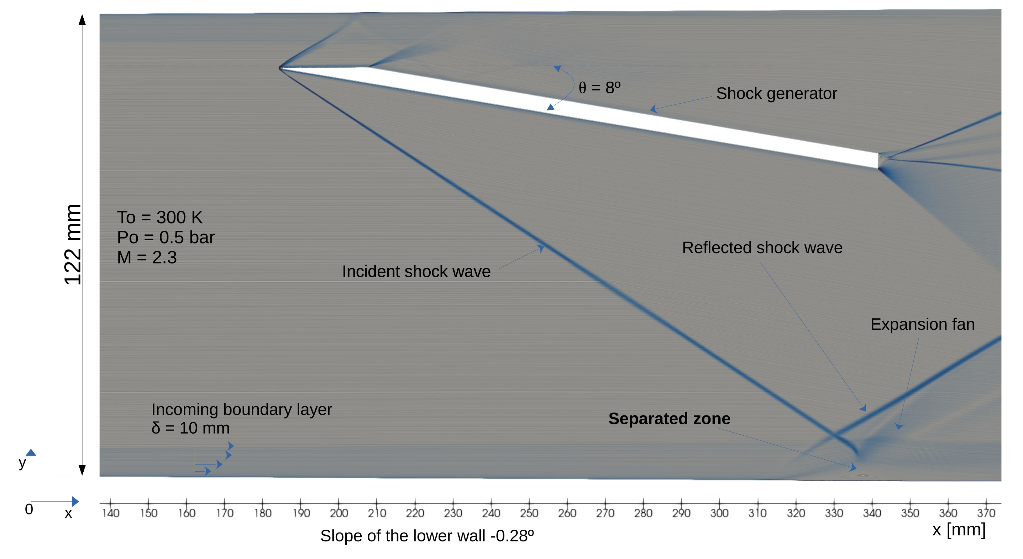
The experimental facility was consist of the the rectangular shaped nozzle (height 120 mm, width 170 mm) designed for a nominal Mach number of . A deflector as a flat plane with a sharp leading edge is held by the wind tunnel upper wall to generate an oblique shock wave which reflects on the lower wall. With the deviation angle of the interaction between the shock and the lower wall boundary layer is strong and the boundary layer fully separates. Figure A1 displays a description of the nozzle in two-dimensional space and associated distribution of the Mach number. Figure A2 shows a zoom near deflector and prime features of the flow topology: incident and reflected shock waves, incoming boundary layer, separation and relaxation zones with expansion fan. The boundary layer is fully turbulent and develops on a lower wall with nearly adiabatic constant wall temperature. Just upstream of the interaction ( mm), it has thickness of 10 mm. The stagnation pressure and temperature being respectively equal to Pa and 300 K, the Reynolds number based on the momentum thickness is about .
Figure A1.
Description of the wind tunnel with installed deflector and isocontours of the Mach number
Figure A1.
Description of the wind tunnel with installed deflector and isocontours of the Mach number
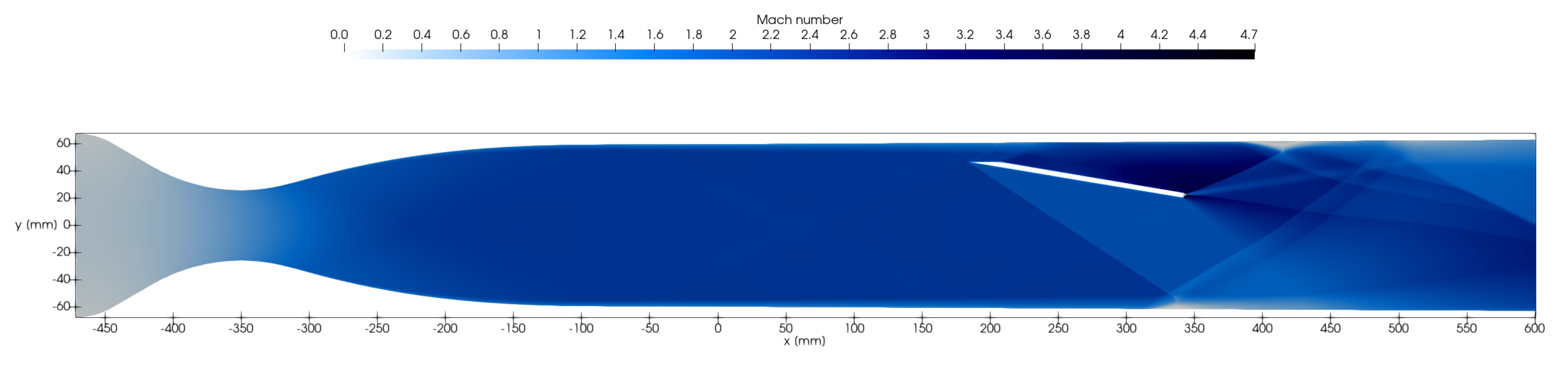
Figure A2.
Sketch of the turbulent shock wave/boundary layer interaction with description of main flow features
Figure A2.
Sketch of the turbulent shock wave/boundary layer interaction with description of main flow features
Both Particle Image Velocimetry (PIV hereafter) and Laser Doppler Velocimetry (LDV hereafter) were used as independent measurement methods. LDV was used mainly for comparisons with PIV, and by cross- check, to validate PIV measurements. The flow was seeded with particles of incense smoke. Test through a shock wave showed that their size is about 1 micron, and provides sufficient resolution. A PIV/LDA cross- check in the incoming boundary layer showed a good agreement of mean velocity, even at distances as small as . This comparison suggests that the longitudinal velocity is measured with a typical accuracy of . The level of background turbulence in the outer flow is essentially due to aerodynamic noise radiated by the boundary layers. Its level is less than for velocity turbulence intensity. For these experiments we can consider two-dimensionality of the flow, since it was found that a the span-wise variations of the velocity are less than m/s, i.e. less than of the bulk velocity and therefore at the limit of the accuracy of measurements [48]. Further details and experimental data are available online via the ERCOFTAC knowledge base Wiki [49].
Appendix A.2. Brief Description of the Computational Grids, Boundary Condition and Run Matrix for Numerical Exercises
The following grid strategy was applied. The computational domain was the entire wind tunnel including the nozzle and the deflector. The initial unstructured grid (A0) was constructed from homogeneous, predominantly quad elements with a characteristic linear size of mm and viscous subgrid layers attached to the walls (with the following parameters: the height of the first cell is mm, the number of layers is 20, and the growth factor of ). The second grid (A1) was constructed in the same way, when the characteristic linear cell size was adapted to mm, and the parameters of the viscous subgrid were: the height of the first cell is mm, the number of layers is 20, and the growth factor is ). It should be noted that such parameters provided already for the initial grid the distribution within about 1. In addition, for these two grids a fairly good grid dependence of the solution was achieved, when the variance for local velocity distributions was only a few percent.
The initial and boundary conditions were set as follows. At the wind tunnel inlet, the total pressure and temperature were set, and the turbulence intensity was low (about ). The outlet conditions are not critical for this problem, since supersonic flow is observed at the outlet. The initial conditions simulate the situation when the shutter from the chamber with parameters and is suddenly opened. The run matrix is given in Table A1. We used all three numerical approaches to solve the viscous, compressible Navier-Stokes equations given in Sec. Section 3.1 and two turbulence models, SA and RKE, respectively. Thermodynamic properties of the gas, such as viscosity and heat capacity, are set by functional dependencies on temperature, also described in Sec. Section 3.1. Heat transfer with the external environment is not taken into account, assuming adiabatic walls, which approximately corresponds to experimental conditions.

Table A1.
Summary of the RANS cases to investigate the turbulent shock wave/boundary layer interaction problem: id – case index, Method – pressure-based, density-based or hybrid, Mesh – A0 or A1, TM – turbulence model, RKE or SA, respectively
Table A1.
Summary of the RANS cases to investigate the turbulent shock wave/boundary layer interaction problem: id – case index, Method – pressure-based, density-based or hybrid, Mesh – A0 or A1, TM – turbulence model, RKE or SA, respectively
| id | Method | Mesh | TM |
|---|---|---|---|
| A0-PB-RKE | pressure-based | A0 | RKE |
| A1-PB-RKE | pressure-based | A1 | RKE |
| A1-PB-SA | pressure-based | A0 | SA |
| A1-DB-RKE | density-based | A1 | RKE |
| A1-DB-SA | density-based | A1 | SA |
| A1-H-SA | hybrid | A1 | SA |
Figure A3.
Stream-wise (a) and vertical (b) velocity profiles in the upstream boundary layer ( and 291 mm) and along the interaction region (, 350 and 370 mm)
Figure A3.
Stream-wise (a) and vertical (b) velocity profiles in the upstream boundary layer ( and 291 mm) and along the interaction region (, 350 and 370 mm)
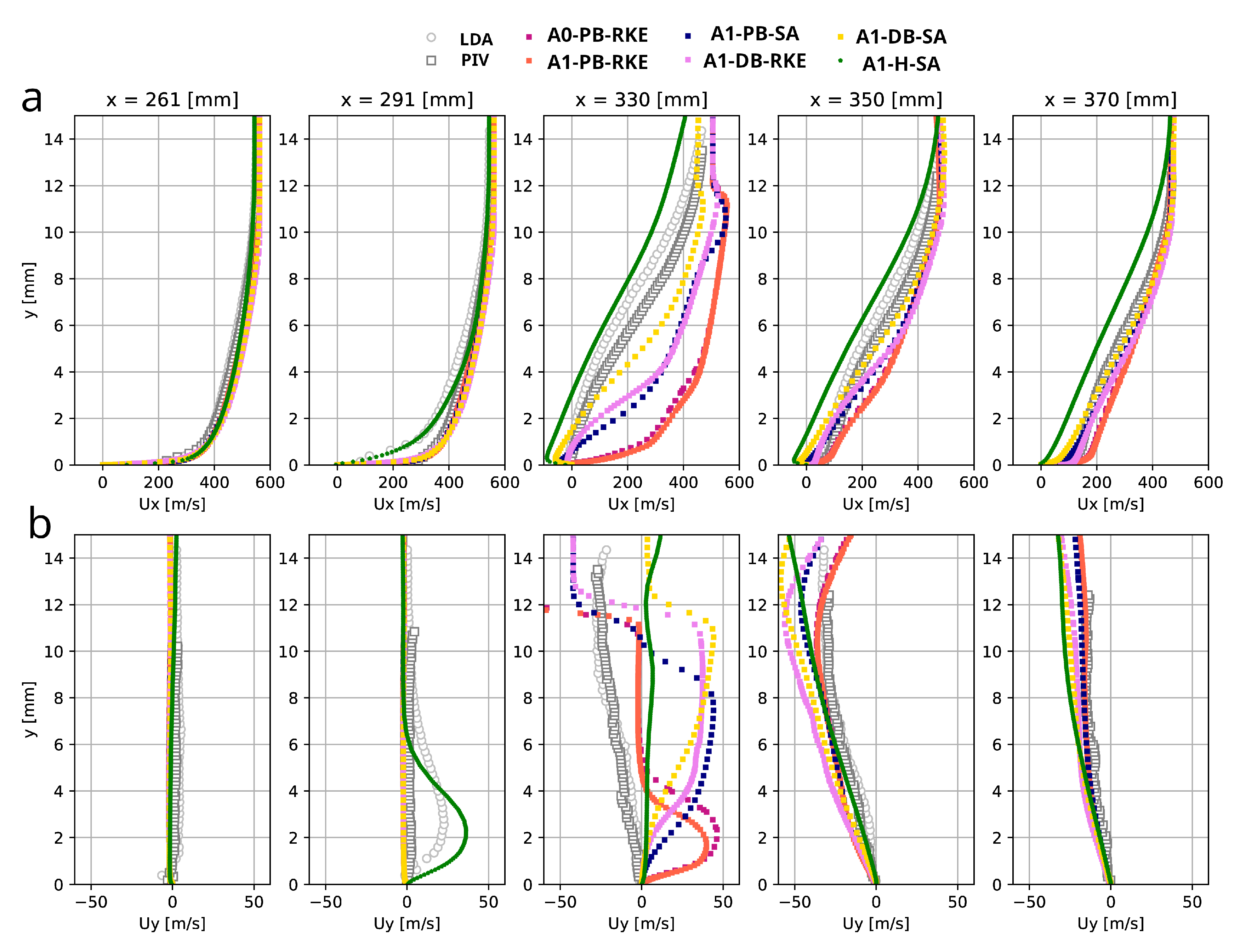
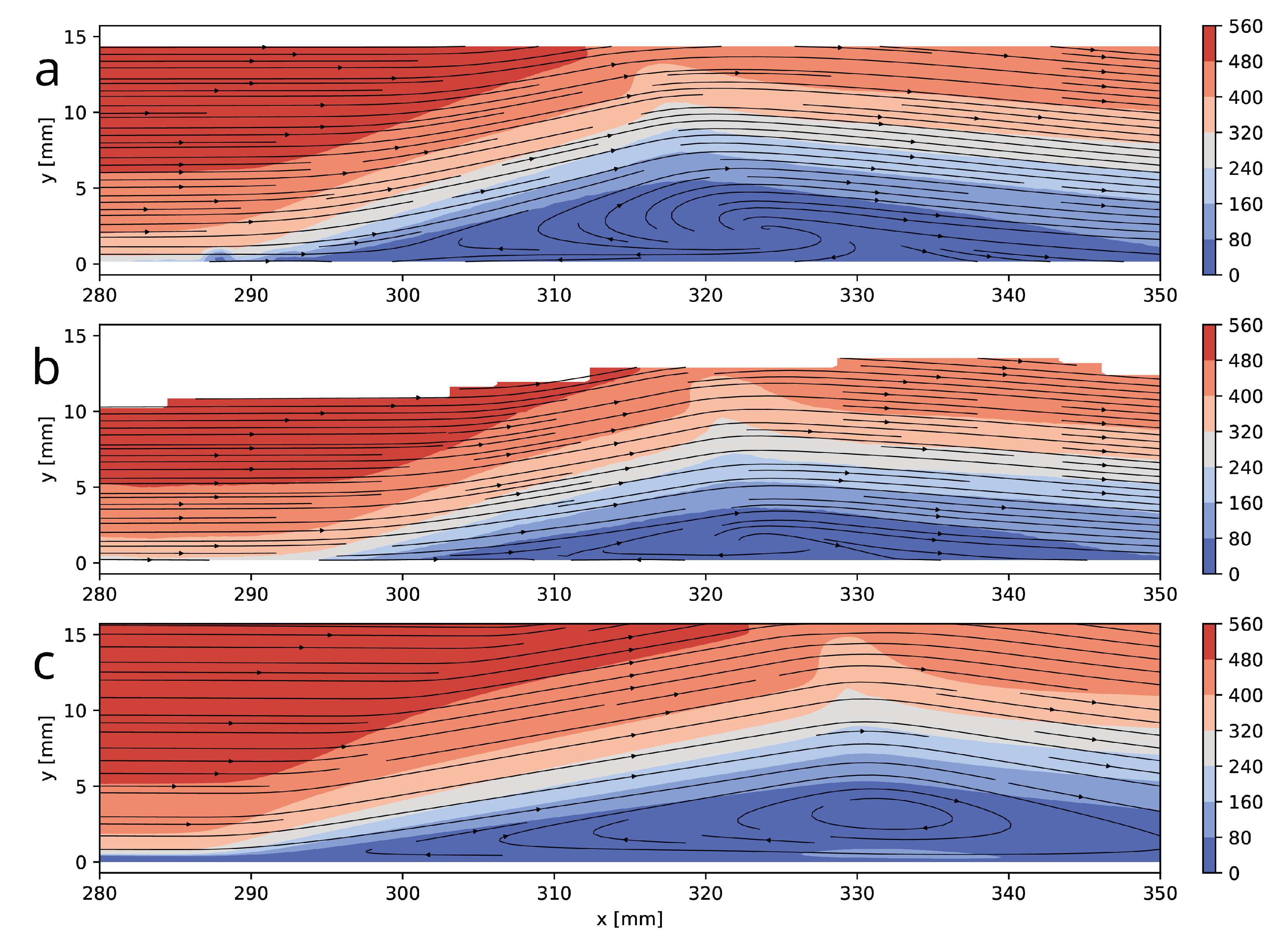
Figure A4.
Visualization of the separated zone: streamlines obtained experimentally by LDV (a) and PIV (b) and numerically (c, case A1-H-SA) colored by the velocity magnitude
Figure A4.
Visualization of the separated zone: streamlines obtained experimentally by LDV (a) and PIV (b) and numerically (c, case A1-H-SA) colored by the velocity magnitude
Appendix A.3. Results and Discussion
The main results are summarized in Figure A3, which presents comparison of the both LDV and PIV experiments and numerical results for the stream-vise () and vertical () velocities profiles at five different axial states, mm, 291 mm, 330 mm, 350 mm and 370 mm. One can see that satisfactory agreement both for and was achieved between RANS and measurements at the positions closed to the upstream and downstream location of the separation bubble. At the middle part of the reticulation zone (approx., mm), all simulations are failed to reproduce dimensions of the separated zone. Figure A4 demonstrates streamlines obtained experimentally (both LDV and PIV) and numerically (case A1-H-SA), where it can be observed some differences in the form of separated zones. There are also a few additional observations that can be made. The pressure-based and density-based approached revealed quite similar results, meanwhile the hybrid approach a little different from them. The results computed using the SA and RKE turbulence models are quite consistent as well. Of course, the low frequency unsteadiness like the fluctuations induced by the shock motion (frequency about 500 Hz) or the large broadband eddies in the separated zone induced by Kelvin-Helmholtz instability (about 6 kHz). was not captured by the RANS methods.
In practice, all methods capture the primary flow features, such as incident and reflected shock waves, expansion fans, and separation and relaxation zones, reasonably well within the mathematical frameworks defined by the imposed assumptions. The predicted mean velocity field in the upstream boundary layer, as well as the shock wave/boundary layer interaction downstream, also shows satisfactory agreement, indicating that the current numerical methods are capable of modeling this class of problems.
References
- Sedda, S., Sardu, C., Lasagna, D., Iuso, G., Donelli, R.S., Gregorio, F. De., Trapped vortex cell for aeronautical applications: flow analysis through PIV and Wavelet transform tools, 10th Pacific Symposium on Flow Visualization and Image Processing, Naples, Italy (2015).
- Lysenko, D.A., Donskov, M., Ertesvåg, I.S., Large-eddy simulations of the flow past a bluff-body with active flow control based on trapped vortex cells at Re = 50000, Ocean Eng, 280, 114496 (2023).
- Ringleb, F.O., Separation control by trapped vortices. In: Boundary Layer and Flow Control, Ed. Lachmann G.V., Pergamon Press (1961).
- Kasper, W., Aircraft wing with vortex generation, US Patent No. 3831885 (1974).
- Kruppa, E.W., A Wind Tunnel Investigation of the Kasper Vortex Concept, AIAA, 77-310 (1977).
- Savitsky, A.I., Schukin, L.N., Karelin, V.G., Mass, A.M., Pushkin, R.M., Shibamov, A.P., Schukin, I.L., Fischenko, S.V., Method for controlling boundary layer on an aerodynamic surface of a flying vehicle, US Patent No. 5417391 (1995).
- Ermishin, A.V., Isaev, S.A., Flow control past bodies with Vortex Cells applied to a blended wing-body aircraft (Numerical and Physical Modeling)(In Russian). St.Petersburg University of Civil Aviation, Saint-Petersburg, Moscow.
- Donelli, R., Gregorio, F. De, Iannelli, P., Flow separation control by trapped vortex, AIAA 2010-1409 (2010).
- Isaev, S.A., Aerodynamics of thickened bodies with vortex cells (Numerical and Physical Modeling)(In Russian). St.Petersburg Polytechnic University, Saint-Petersburg. (2016).
- Lysenko D.A., On numerical simulations of turbulent flows over a bluff body with aerodynamic flow control based on trapped vortex cells: viscous effects, Fluids. 2025; 10(5):120. [CrossRef]
- Lysenko, D.A., Donskov, M., Ertesvåg, I.S., Large-eddy simulations of the flow over a semi-circular cylinder at Re = 50000, Comput Fluids, 228 (2021) 10505.
- Chase, M., NIST-JANAF Thermochemical tables, 4th Ed., J. Phys. Chem. Ref. Data, Monographs and Supplements, 9 (1998).
- McBride, B.J., Zehe, M.J., Gordon, S., NASA Glenn coefficients for calculating thermodynamic properties of individual species. Technical Report NASA/TP-2002-211556, National Aeronautics and Space Administration (2002) URL: https://ntrs.nasa.gov/citations/20020085330.
- Spalart, P. and S. Allmaras, S., A one-equation turbulence model for aerodynamic flows, Technical Report AIAA-92-0439 (1992).
- Shih, T.H., Liou, W., Shabbir, A., Yang, Z., Zhu, J. A new k eddy-viscosity model for high Reynolds number turbulent flows - model development and validation, J Comput Fluids 24(3), 227-38 (1995).
- Dacles-Mariani, J., Zilliac, G.G., Chow, J.S., Bradshaw, P., Numerical/Experimental study of a wingtip vortex in the near field, AIAA Jl, 33(9), 1561-1568 (1995).
- Sarkar, S, Balakrishnan, L., Application of a Reynolds-stress turbulence model to the compressible shear layer, ICASE Report 90-18, NASA CR 182002 (1990).
- ANSYS FLUENT 2021SRb. Theory guide. Tech. rep., Ansys Inc. (2021).
- Weller, H.G., Tabor, G., Jasak, H., Fureby, C., A tensorial approach to computational continuum mechanics using object-oriented techniques, J Comput Phys, 12(6), 620-631 (1998).
- Chorin, A.J., Numerical Solution of the Navier-Stokes Equations, Math Comput., 22(104), 745-762 (1968).
- Issa, R., Solution of the implicitly discretized fluid flow equations by operator splitting, J Comput Phys, 62, 40-65 (1986).
- Geurts, B, Elements of direct and large-eddy simulation, R.T.Edwards, Philadelphia (2004).
- Hutchinson B, Raithby G. A multigrid method based on the additive correction strategy, J Numer Heat Transfer, 9, 511-37 (1986).
- Godunov, S.K., I. Bohachevsky, I., Finite difference method for numerical computation of discontinuous solutions of the equations of fluid dynamics, Matematičeskij sbornik, 47(89) (3), 271-306 (1959).
- Toro, E.F., Riemann Solvers and Numerical Methods for Fluid Dynamics, 3rd Edition, Springer-Verlag Berlin Heidelberg (2009).
- Liou, M.-S., Steffen, C., A new flux splitting scheme, J Comput Phys, 107, 23-39 (1993).
- Ferziger, J.H., Peric, M., Computational Methods for Fluid Dynamics // 3rd edition, Berlin; Heidelberg; New York; Barcelona; Hong Kong; London; Milan; Paris; Tokyo: Springer, (2002).
- Kurganov, A., Noelle, S., Petrova, G., Semi-discrete central-upwind schemes for hyperbolic conservation laws and Hamilton–Jacobi equations, SIAM J Sci Computing, 23m 707-740 (2001).
- Kraposhin, M., Bovtrikova, A., Strijhak, S., Adaptation of Kurganov-Tadmor numerical scheme for applying in combination with the PISO method in numerical simulation of flows in a wide range of Mach numbers, Procedia Computer Science, 66, 43-52 (2015).
- Van Leer, B., Towards the ultimate conservative difference scheme. II. Monotonicity and conservation combined in a second-order scheme. J Comput Physics, 14, 361-370 (1974).
- Wolfshtein, M., The velocity and temperature distribution of one-dimension flow with turbulence augmentation and pressure gradient, I J Heat Mass Transfer, 12, 301-318 (1969).
- Chen, H.C., Patel, V.C., Near-wall turbulence models for complex flows including separation, AIAA J, 26(6), 641-648 (1988).
- Jongen, T., Simulation and modeling of turbulent incompressible flows, PjD thesis, EPF Lausanne, Lausanne, Switzerland (1992).
- Menter, F., Ferreira, J.C., Esch, T., Konno, B., The SST turbulence model with improved wall treatment for heat transfer predictions in gas turbines. Proceedings of the International Gas Turbine Congress, 2-7 (2003).
- Lysenko, D.A. Large-eddy simulation of the flow past a circular cylinder at Re = 130,000: Effects of numerical platforms and single- and double-precision arithmetic, Fluids, 10, 4 (2025).
- Isaev, S.A., Baranov, P.A., Kudryavtsev, N.A., Lysenko, D.A., Usachov, A.E., Complex analysis of turbulence models, algorithms, and grid structures at the computation of recirculating flow in a cavity by means of VP2/3 and FLUENT packages. Part 2. Estimation of models adequacy, Thermophysics and Aeromechanics, 13(1), 55-65 (2006).
- Isaev, S.A., Baranov, P.A., Kudryavtsev, N.A., Lysenko, D.A., Usachov, A.E., Complex analysis of turbulence models, algorithms, and grid structures at the computation of recirculating flow in a cavity by means of VP2/3 and FLUENT packages. Part 1. Scheme factors influence, Thermophysics and Aeromechanics, 12(4), 549-569 (2005).
- Isaev, S.A., Baranov, P.A., Kudryavtsev, N.A., Lysenko, D.A., Usachov, A.E., Comparative analysis of the calculation data on an unsteady flow around a circular cylinder obtained using the VP2/3 and FLUENT packages and the Spalart-Allmaras and Menter turbulence models, J Engineering Physics and Thermophysics, 78(6), 1199-1213 (2005).
- Isaev S , Baranov P , Popov I , Sudakov A , Usachov A , Guvernyuk S , et al. Numerical simulation and experiments on turbulent air flow around the semi-circular profile at zero angle of attack and moderate Reynolds number, Comput Fluids, 188:1-17 (2019).
- Lysenko, D.A., Ertesvåg, I.S., Rian, K.E., Modeling of turbulent separated flows using OpenFOAM, Comput. Fluids, 80, 408-422 (2013).
- Lysenko, D.A., Ertesvåg, I.S., Rian, K.E., Towards simulation of far-field aerodynamic sound from a circular cylinder using OpenFOAM, I J Aeroacoustics, 13(1), 141-168 (2014).
- Isaev, S.A. and Lysenko, D.A., Testing of the FLUENT package in calculation of supersonic flow in a step channel, J Engineering Physics and Thermophysics, 78(4), 857-860 (2004).
- Isaev, S.A. and Lysenko, D.A., Testing of numerical methods, convective schemes, algorithms for approximation of flows, and grid structures by the example of a supersonic flow in a step-shaped channel with the use of the CFX and FLUENT packages, J Engineering Physics and Thermophysics, 82(2) 321-326 (2009).
- Garnier, E., Stimulated detached eddy simulation of three-dimensional shock/boundary layer interaction, Shock Waves 19(6), 479-486 (2009).
- Lysenko, D.A. and Isaev, S.A., Calculation of unsteady flow past a cube on the wall of a narrow channel using URANS and the Spalart-Allmaras turbulence model, J Engineering Physics and Thermophysics, 82(3) 488-495 (2009).
- Isaev, S.A., Nikushchenko, D.V., Sudakov, A.G., Yunakov, L.P., Tryaskin, N.V., Control of subsonic flow around a semicircular airfoil with the use of slot suction in vortex cells, J Eng Physics Thermophysics, 98(5) (2025).
- Isaev, S., Nikushchenko, D., Sudakov, A., Tryaskin, N., Egorova, A., Iunakov, L., Usachov, A., Kharchenko, V., Standard and modified SST models with the consideration of the streamline curvature for separated flow calculation in a narrow channel with a conical dimple on the heated wall, Energies, 14, 5038, 1-23 (2021).
- Dussauge J.P., Piponniau S., Shock boundary layer interactions: possible sources of unsteadiness, J Fluids Structures, 24(8), 1166-75 (2008 ).
- The ERCOFTAC Knowledge Base Wiki, https://www.kbwiki.ercoftac.org/w/index.php?title=Abstr:UFR_3-32.
Figure 1.
Schematic flow visualization over a simplified bluff body: (a) without aerodynamic flow control and (b) with integrated AFC system [2]
Figure 1.
Schematic flow visualization over a simplified bluff body: (a) without aerodynamic flow control and (b) with integrated AFC system [2]
Figure 2.
Schematic of a fixed-wing concept with integrated AFC (a) and its flow visualization at , and zero angle of attack. Iso-surfaces of the Q-criterion (, where S is the strain rate and is the vorticity) highlight coherent vortex structures (b). Flow dynamics within the AFC system are illustrated using LIC visualization of the time-averaged velocity field in the central vertical cross-section (c)
Figure 3.
Key design characteristics of a thick airfoil: with and without Trapped Vortex Cells. x, y and z are Cartesian coordinates in the longitudinal, vertical and spanwise directions
Figure 3.
Key design characteristics of a thick airfoil: with and without Trapped Vortex Cells. x, y and z are Cartesian coordinates in the longitudinal, vertical and spanwise directions
Figure 4.
General view of a bluff body with the integrated aerodynamic flow control system and locations of the surface for air suction (a). The flow mechanics over the thick airfoil (b) and airfoil with AFC (c)
Figure 4.
General view of a bluff body with the integrated aerodynamic flow control system and locations of the surface for air suction (a). The flow mechanics over the thick airfoil (b) and airfoil with AFC (c)
Figure 5.
General view of the baseline mesh A0 and computational domain (a). Zoom of A0 (b) and A2 (c) grids in the vicinity of the bluff-body with AFC
Figure 5.
General view of the baseline mesh A0 and computational domain (a). Zoom of A0 (b) and A2 (c) grids in the vicinity of the bluff-body with AFC
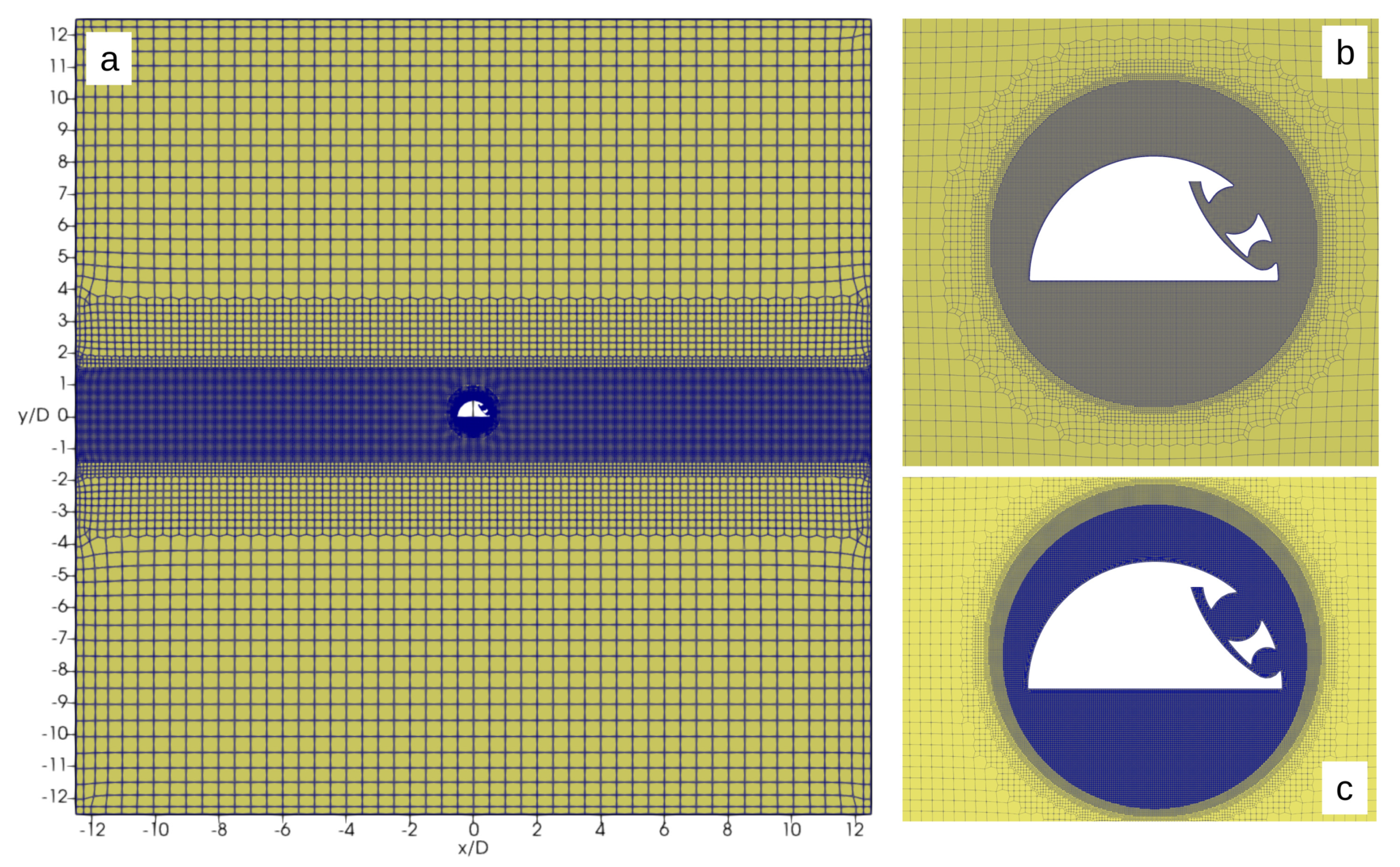
Figure 6.
Isocontours of Mach number (a), density [kg/m3] (b), dynamic viscosity [Pa*s] (c) and thermal conductivity [W/m/K] (d) computed for the flow over a bluff-body with integrated aerodynamic control system at , and zero angle of attack
Figure 6.
Isocontours of Mach number (a), density [kg/m3] (b), dynamic viscosity [Pa*s] (c) and thermal conductivity [W/m/K] (d) computed for the flow over a bluff-body with integrated aerodynamic control system at , and zero angle of attack
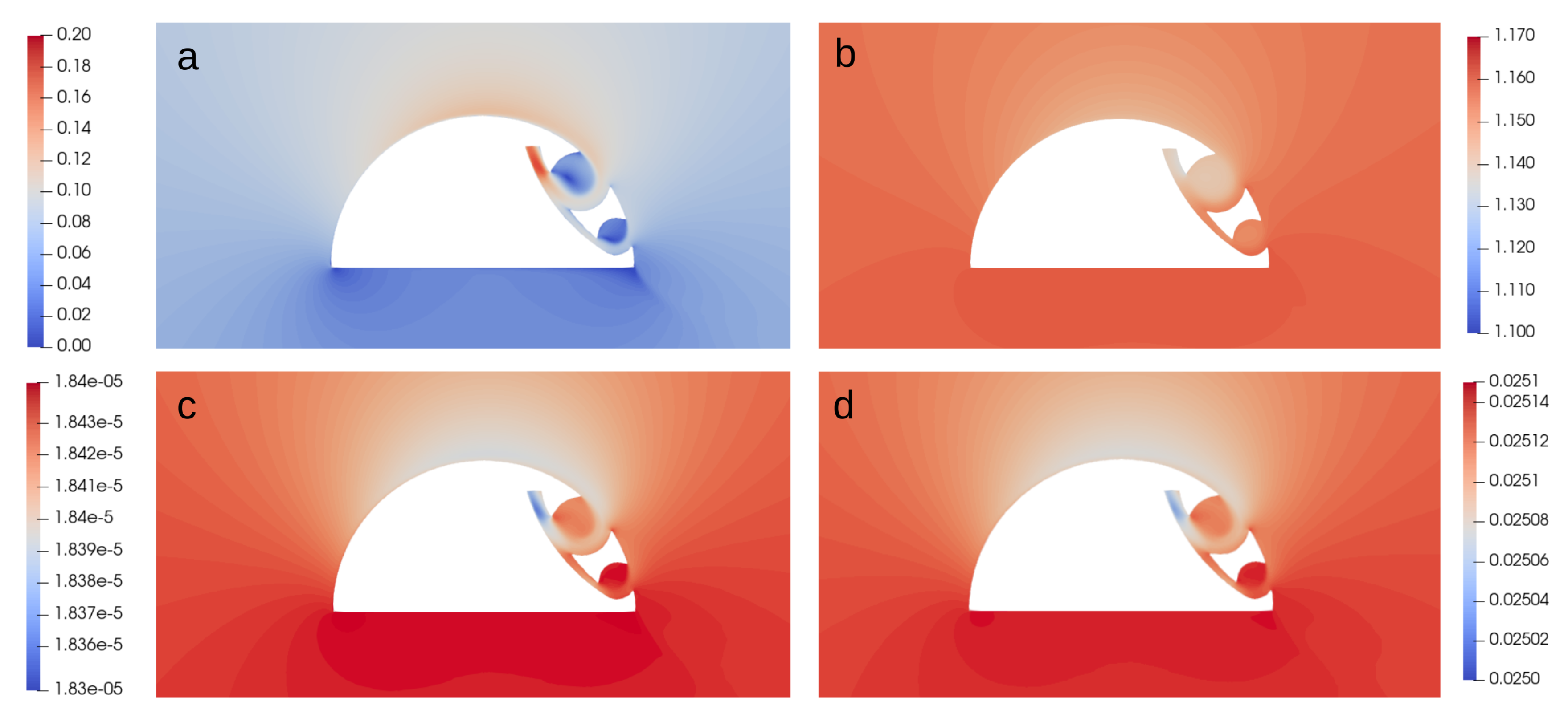
Figure 7.
Dependence of the lift coefficient (a) and aerodynamic quality (b) form the Mach number: runs R00-R07 and R09-R13 from Table 2, respectively. VP23-SST – results obtained by Isaev et al. [46] for the alternative AFC configuration with two TVCs. Schematic differences between two implementations of the AFC system: present work (c) and by Isaev et al. [46] (d)
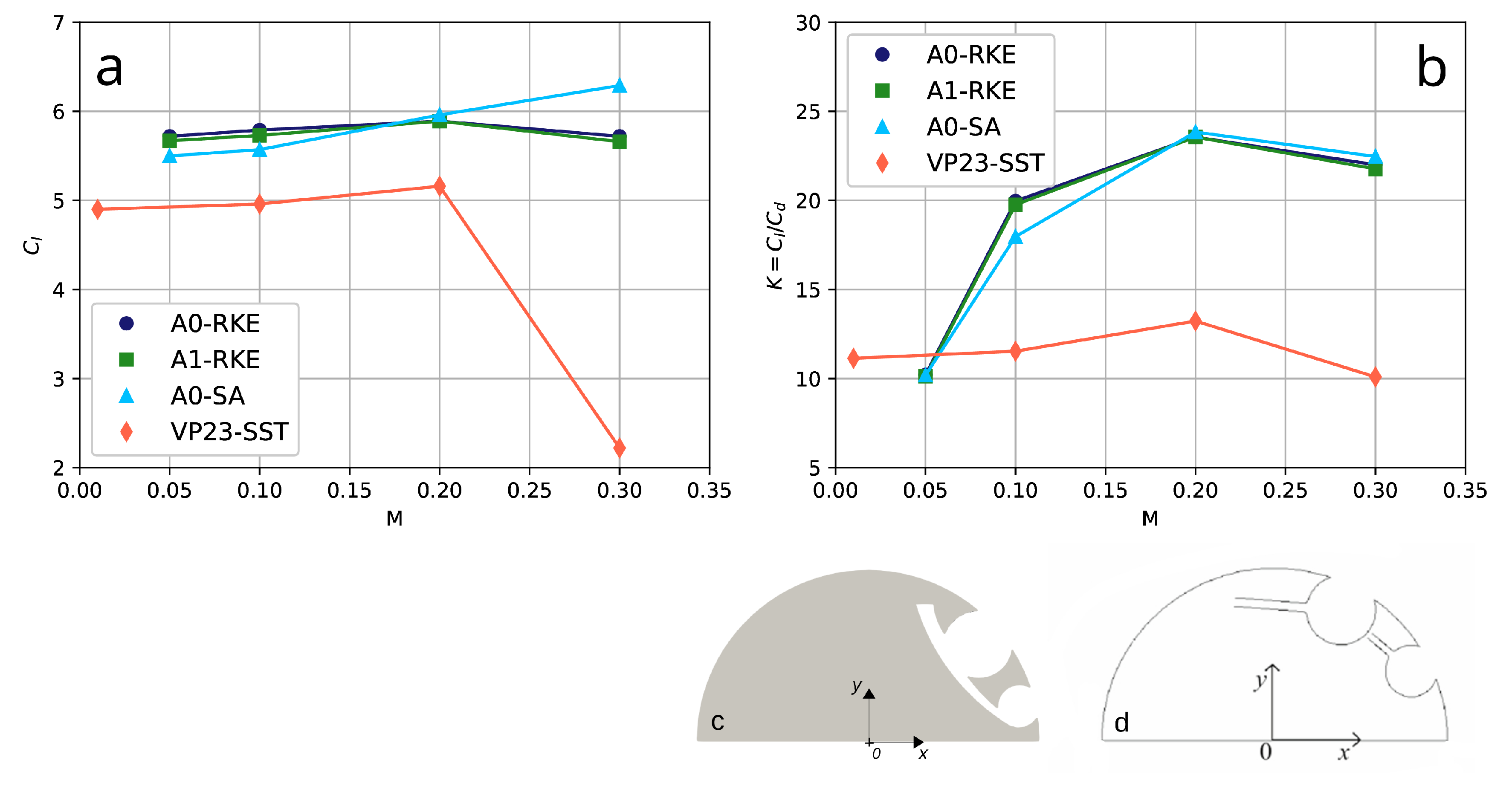
Figure 8.
Dependence of pressure coefficient from Mach number: runs R04-R07 from Table 2
Figure 8.
Dependence of pressure coefficient from Mach number: runs R04-R07 from Table 2
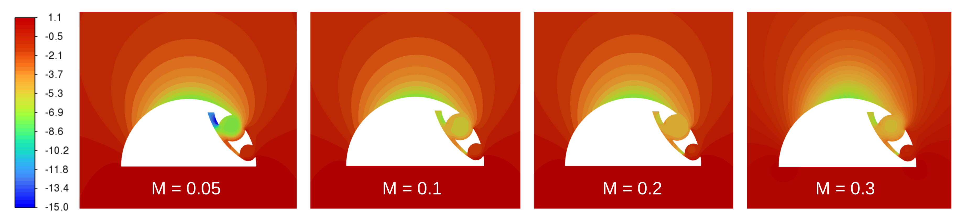
Figure 9.
LIC visualization of the the flow over a bluff body with an integrated aerodynamic control system at , Mach numbers from to and zero angle of attack: runs R04-R07 from Table 2
Figure 9.
LIC visualization of the the flow over a bluff body with an integrated aerodynamic control system at , Mach numbers from to and zero angle of attack: runs R04-R07 from Table 2
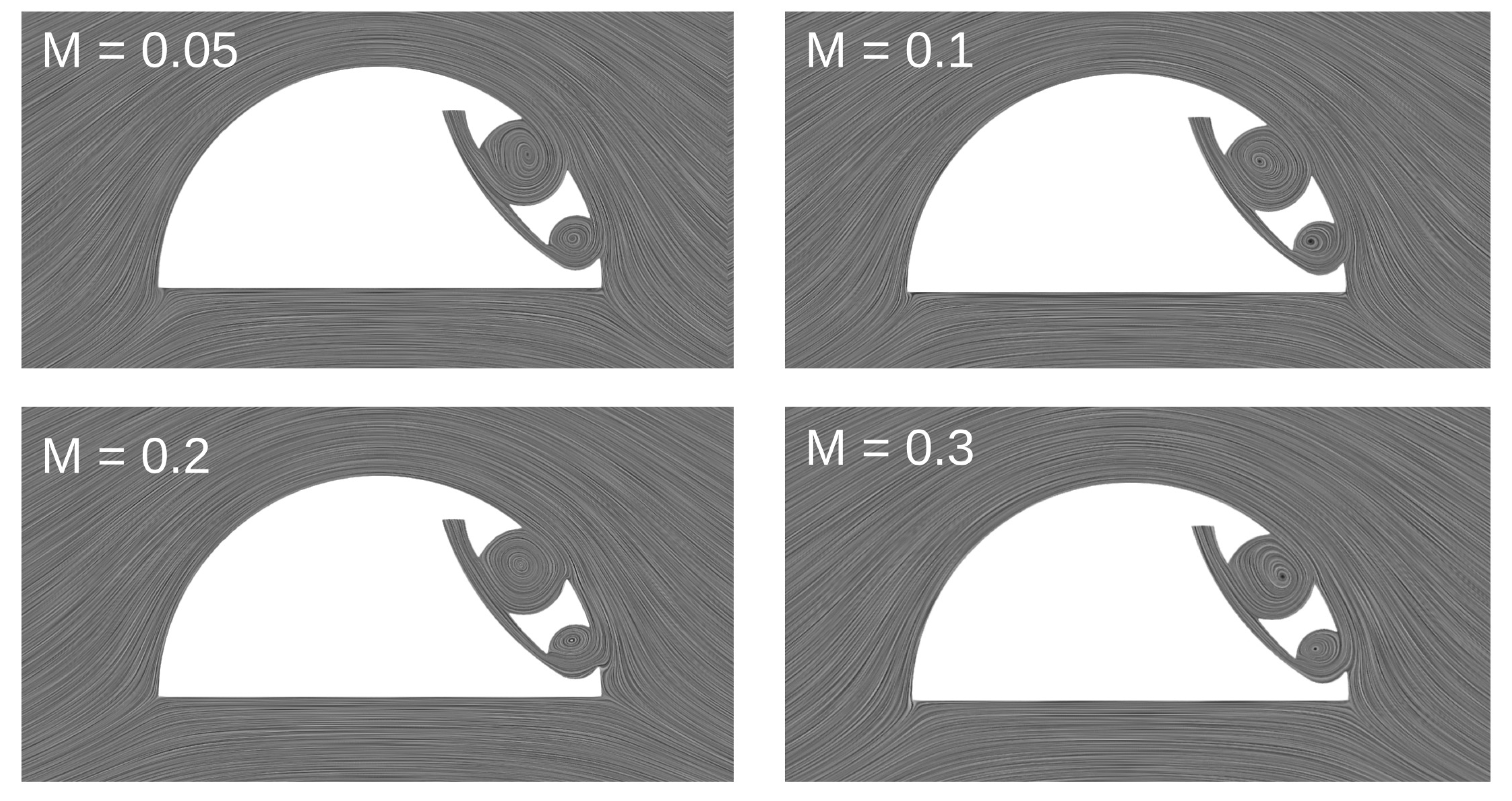
Figure 10.
Isocontours of Mach number of the the flow over a bluff body with an integrated aerodynamic control system at , Mach numbers from to and zero angle of attack: runs R04-R07 from Table 2
Figure 10.
Isocontours of Mach number of the the flow over a bluff body with an integrated aerodynamic control system at , Mach numbers from to and zero angle of attack: runs R04-R07 from Table 2
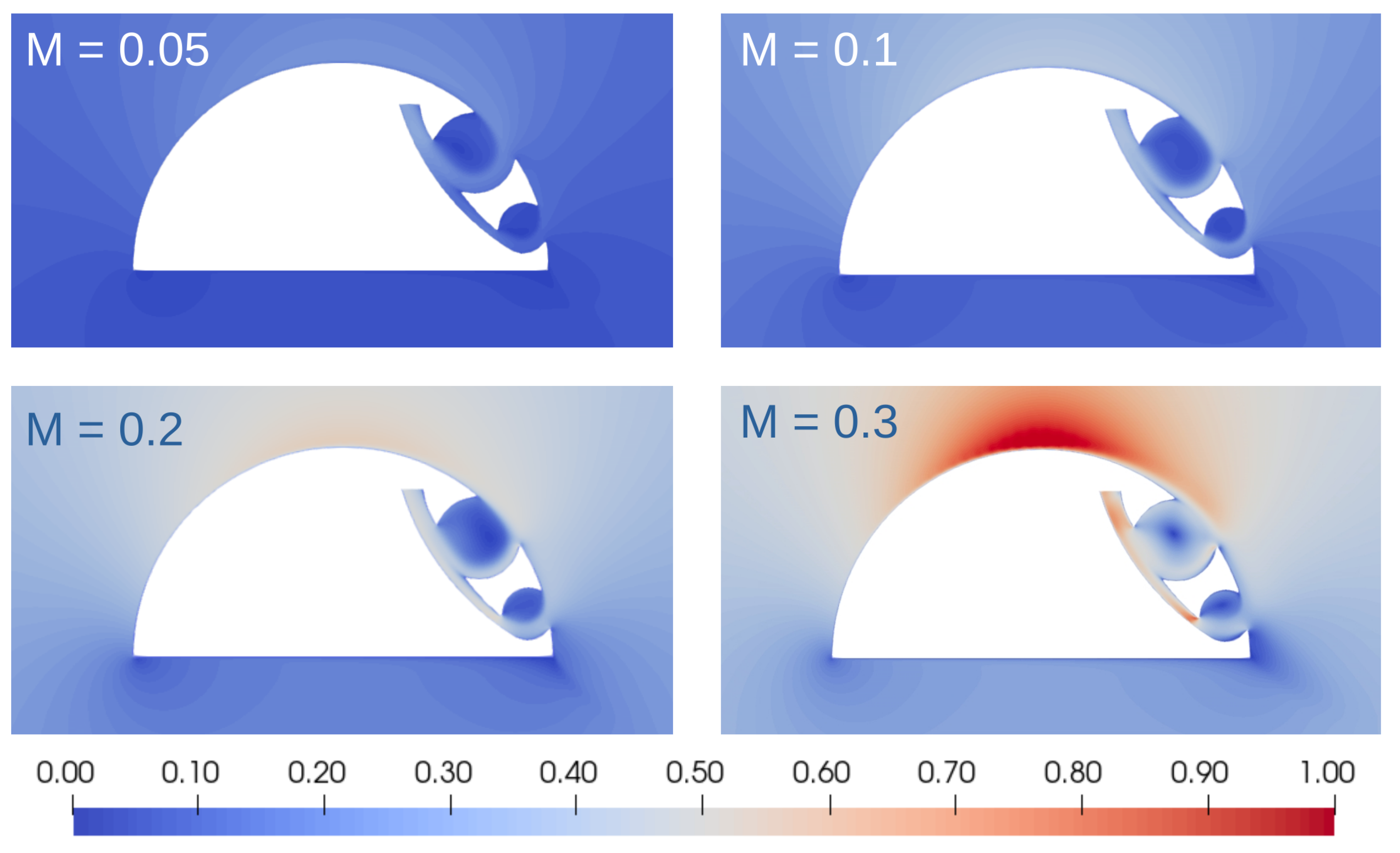
Figure 11.
Isocontours of vorticity magnitude, of the the flow over a bluff body with an integrated AFC at , Mach numbers from to and zero angle of attack: runs R04-R07 from Table 2
Figure 11.
Isocontours of vorticity magnitude, of the the flow over a bluff body with an integrated AFC at , Mach numbers from to and zero angle of attack: runs R04-R07 from Table 2
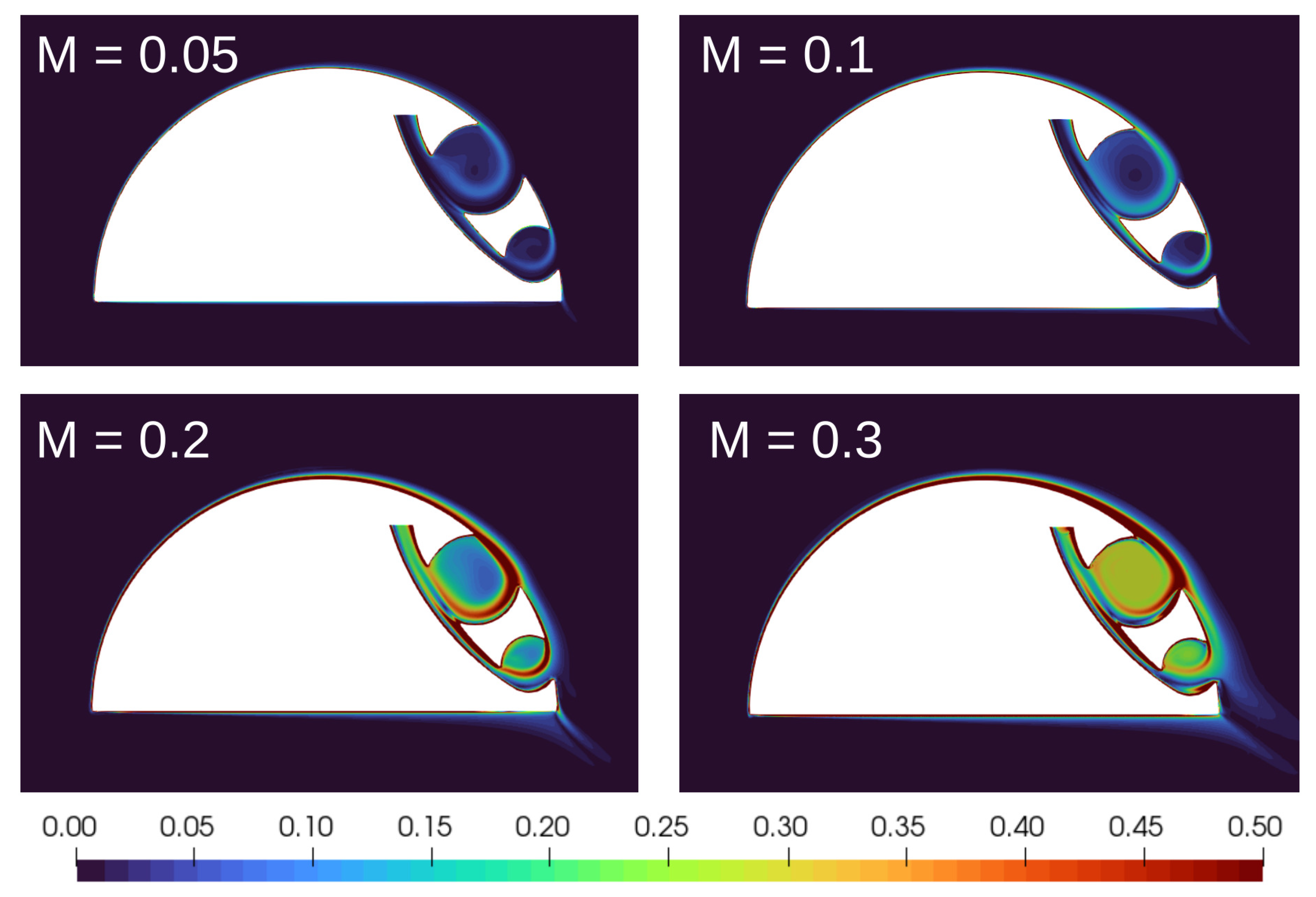
Figure 12.
Sensitivity of the lift (a) and drag (b) coefficients from the angle of attack: runs R19-R24 from Table 2
Figure 12.
Sensitivity of the lift (a) and drag (b) coefficients from the angle of attack: runs R19-R24 from Table 2
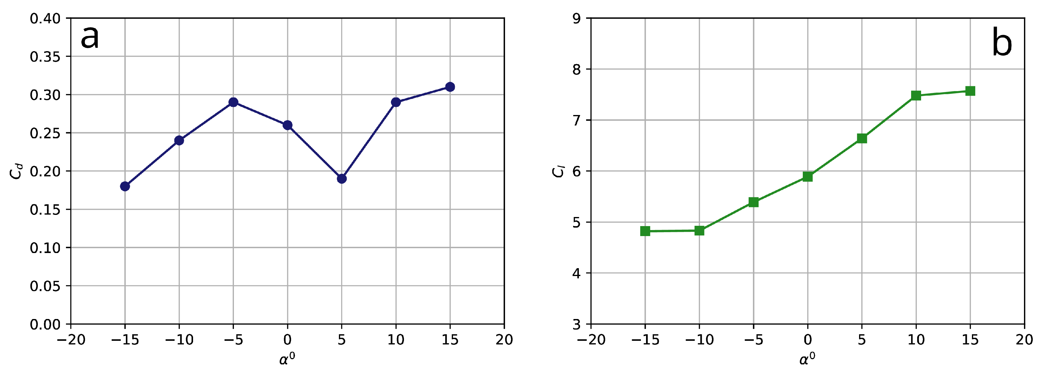
Figure 13.
LIC visualization blended with iso-contours of Mach number of the the flow over a bluff-body with integrated aerodynamic control system at , and different angles of attack within a range of : corresponded cases R19-R24 from Table 2
Figure 13.
LIC visualization blended with iso-contours of Mach number of the the flow over a bluff-body with integrated aerodynamic control system at , and different angles of attack within a range of : corresponded cases R19-R24 from Table 2
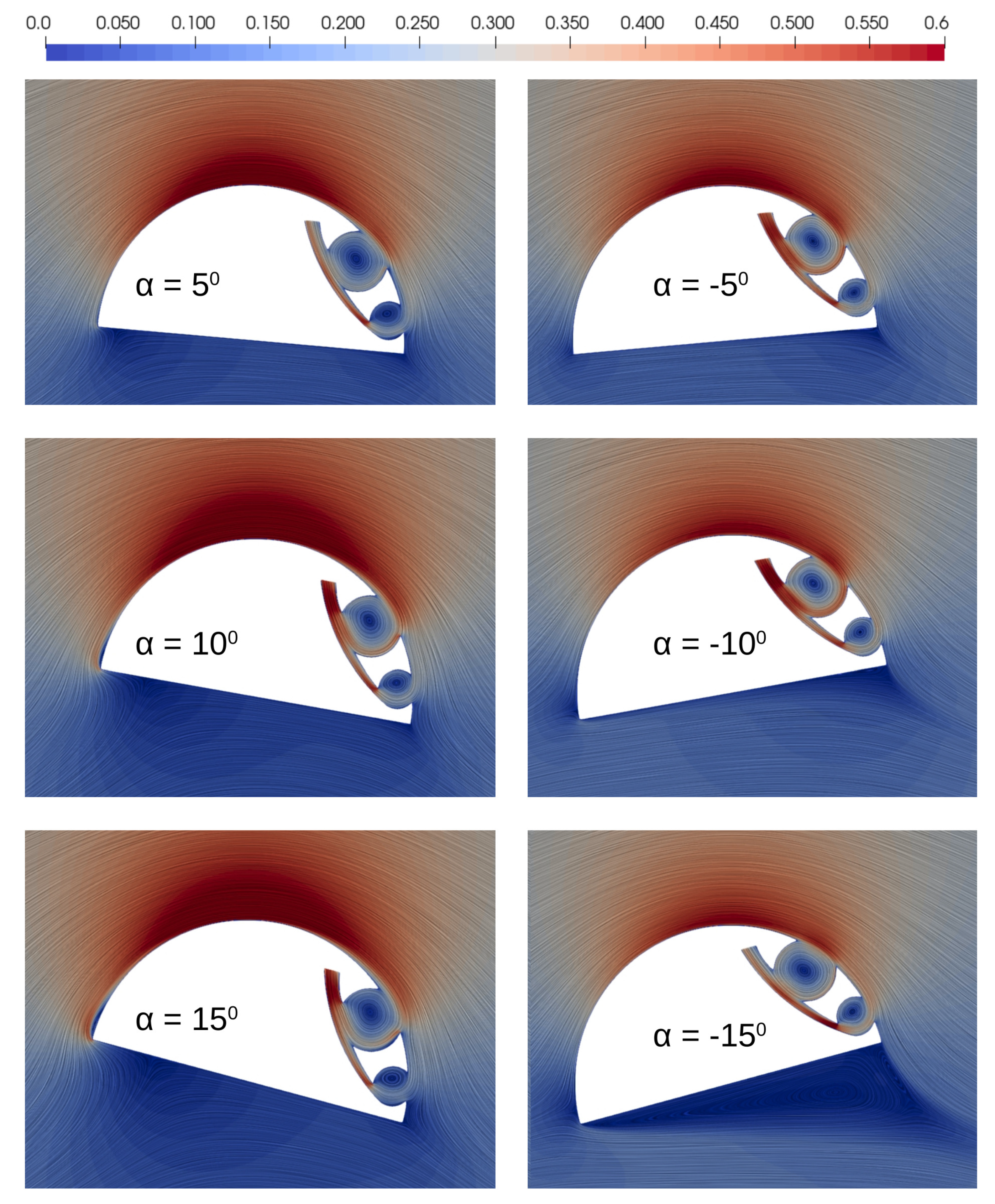
Figure 14.
LIC visualization blended with iso-contours of Mach number of the the flow over a bluff-body with integrated aerodynamic control system at , and zero angle of attack. Sensitivity analysis of the numerical algorithms – pressure-based (R07, R13); density-based (R17, R18) and hybrid (R16) solvers and turbulence models – SA (R13, R18, R16) vs RKE (R07, R17) vs Inviscid case (R25). Case labels are according to Table 2
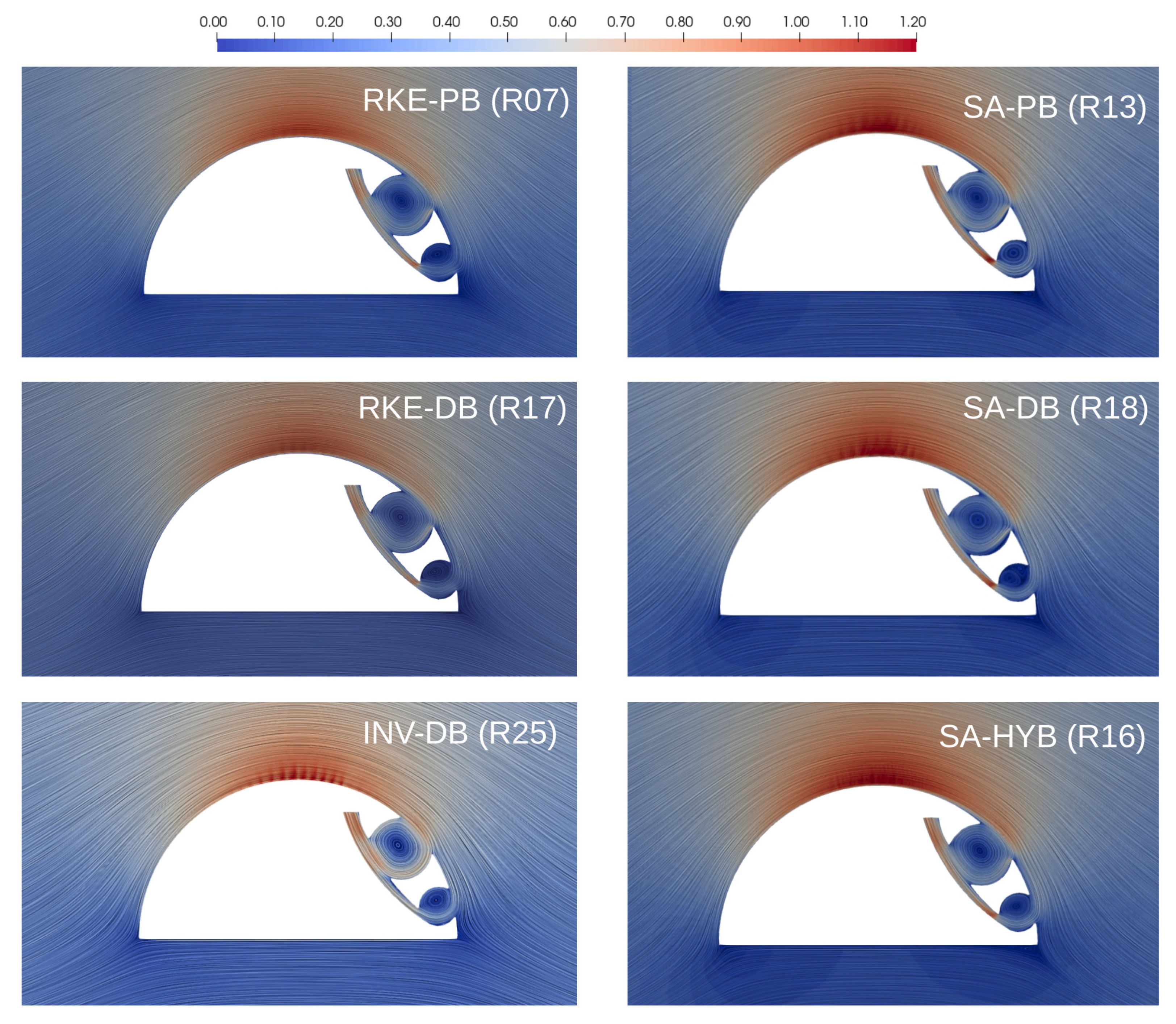
Figure 15.
Local distributions of the velocity (a, b) and vorticity (c, d) magnitudes in a large TVC along two directions (lines AB and CD) perpendicular to each other and intersecting at the center of the vortex cell. Numerical results were obtained for the flow over a thick airfoil with AFC at , and zero angle of attack using various numerical algorithms as pressure-based (R07, R13), density-based (R17, R18) and hybrid (R16) and turbulence models as SA (R13, R1, R16), RKE (R07, R17) and the inviscid case (R25). Case labels are according to Table 2
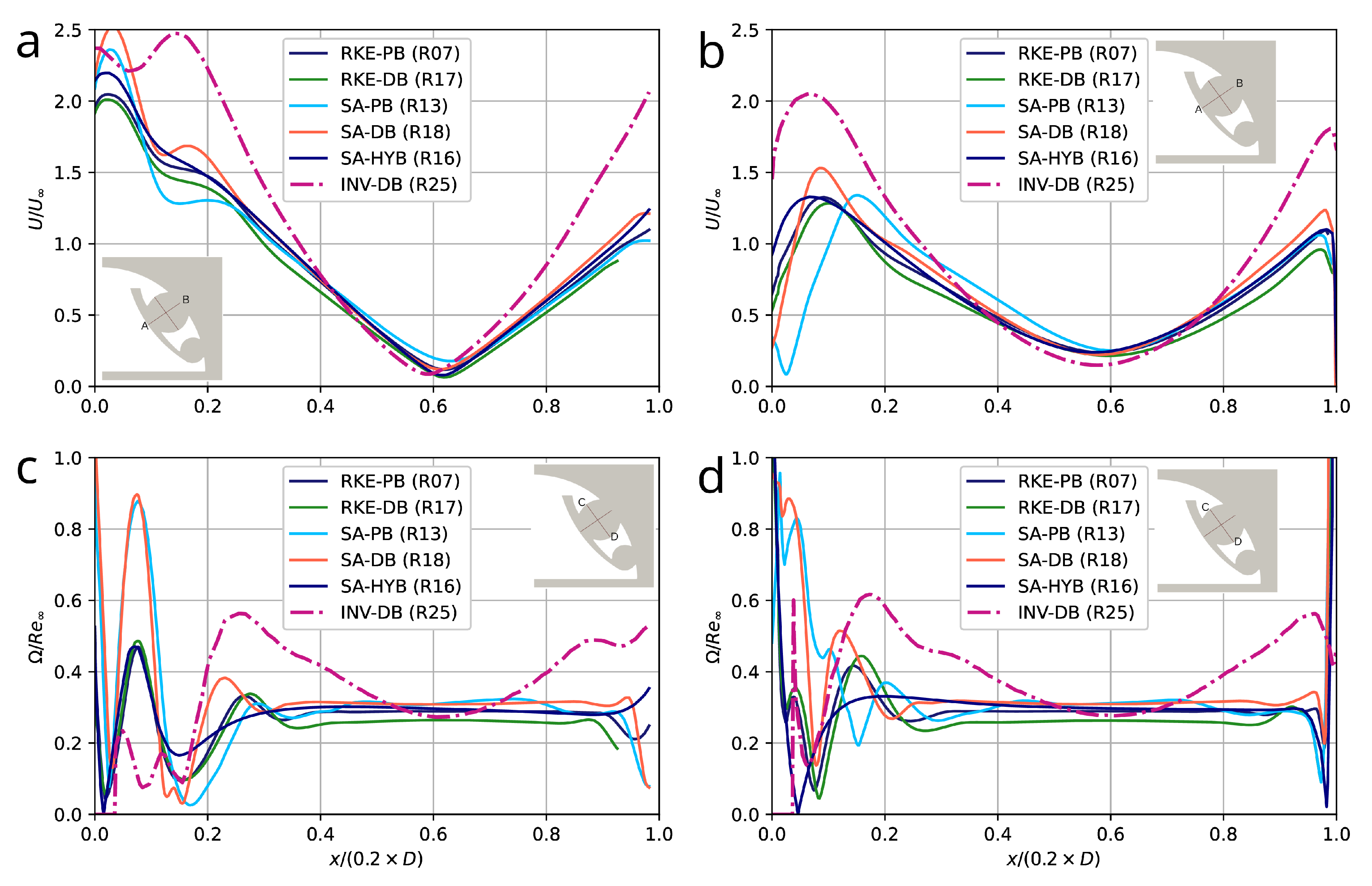
Figure 16.
PDF distributions of at the surface of the bluff-body with AFC computed by the RANS approach at on different grids: runs R12-R14 according to Table 2
Figure 16.
PDF distributions of at the surface of the bluff-body with AFC computed by the RANS approach at on different grids: runs R12-R14 according to Table 2
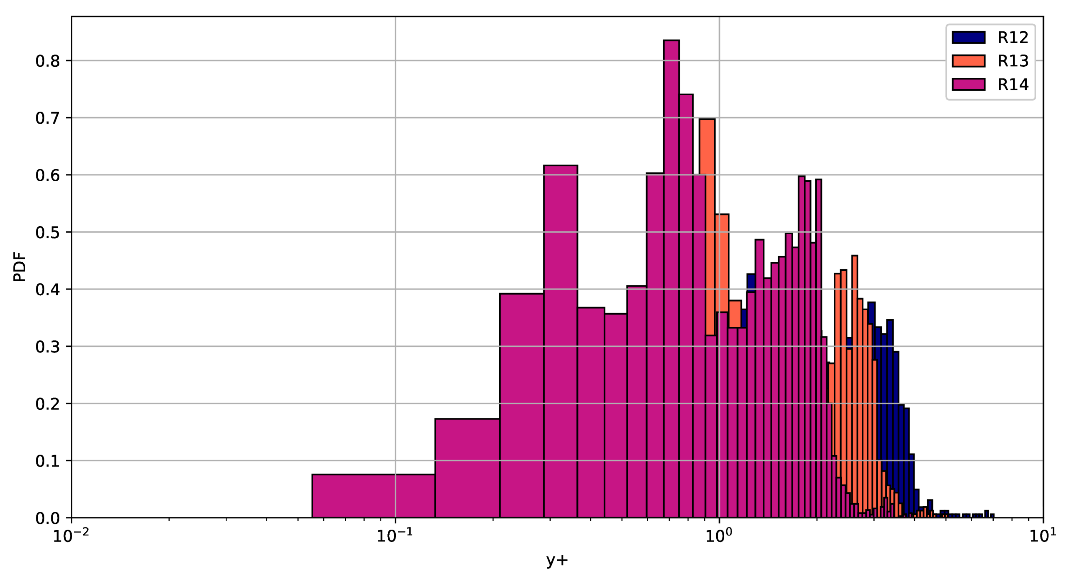
Table 1.
Summary of the free-stream parameters using in the present simulations depending for different Mach numbers as a function of the bluff-body attitude above sea level
Table 1.
Summary of the free-stream parameters using in the present simulations depending for different Mach numbers as a function of the bluff-body attitude above sea level
| h [m] | [kg/m3] | [Pa] | [K] | [m/s] | M |
|---|---|---|---|---|---|
| 0 | 1.16 | 100,000 | 300 | 17 | 0.05 |
| 1,000 | 1.14 | 89,800 | 281 | 35 | 0.1 |
| 5,000 | 0.74 | 54,500 | 255 | 65 | 0.2 |
| 10,000 | 0.42 | 26,500 | 222 | 90 | 0.3 |
Table 2.
Summary of the simulation cases for the fixed Reynolds number investigating the sensitivity of the AFC concept to Mach number: G – grid with related level of refinement (A0, A1 or A2), NM – numerical method (pressure-based (PB), density-based (DB), hybrid (HB) or VP2/3 [46]), TM – turbulence model (RKE, SA, SST or inviscid case, INV), M – Mach number, – angle of attack, , and represent drag, lift coefficients and aerodynamic quality, respectively, – static pressure drop set for air suction
| Run | G | NM | TM | M | [kPa] | Notes | ||||
|---|---|---|---|---|---|---|---|---|---|---|
| AFC-RANS-A1 | A1 | PB | RKE | 0.05 | 0.82 | 4.86 | 6.00 | -2 | [10] | |
| R00 | A0 | PB | RKE | 0.05 | 0.56 | 5.72 | 10 | -2 | ||
| R01 | A0 | PB | RKE | 0.1 | 0.29 | 5.79 | 20 | -4 | ||
| R02 | A0 | PB | RKE | 0.2 | 0.25 | 5.89 | 24 | -8 | ||
| R03 | A0 | PB | RKE | 0.3 | 0.26 | 5.72 | 22 | -10 | ||
| R04 | A1 | PB | RKE | 0.05 | 0.57 | 5.67 | 10 | -2 | ||
| R05 | A1 | PB | RKE | 0.1 | 0.33 | 5.73 | 17 | -4 | ||
| R06 | A1 | PB | RKE | 0.2 | 0.26 | 5.89 | 23 | -8 | ||
| R07 | A1 | PB | RKE | 0.3 | 0.26 | 5.66 | 22 | -10 | ||
| R08 | A2 | PB | RKE | 0.3 | 0.25 | 5.66 | 23 | -10 | ||
| R09 | A0 | PB | SA | 0.05 | 0.54 | 5.5 | 10 | -2 | ||
| R10 | A0 | PB | SA | 0.1 | 0.31 | 5.57 | 18 | -4 | ||
| R11 | A0 | PB | SA | 0.2 | 0.25 | 5.96 | 24 | -8 | ||
| R12 | A0 | PB | SA | 0.3 | 0.28 | 6.29 | 23 | -10 | ||
| R13 | A1 | PB | SA | 0.3 | 0.27 | 6.21 | 23 | -10 | ||
| R14 | A2 | PB | SA | 0.3 | 0.26 | 6.2 | 24 | -10 | ||
| R15 | A0 | HB | SA | 0.3 | 0.28 | 6.27 | 23 | -10 | ||
| R16 | A1 | HB | SA | 0.3 | 0.27 | 6.34 | 24 | -10 | ||
| R17 | A1 | DB | RKE | 0.3 | 0.25 | 5.59 | 22 | -10 | ||
| R18 | A1 | DB | SA | 0.3 | 0.24 | 6.17 | 28 | -10 | ||
| R19 | A1 | PB | RKE | 0.2 | 0.18 | 4.82 | 27 | -11 | ||
| R20 | A1 | PB | RKE | 0.2 | 0.24 | 4.83 | 20 | -11 | ||
| R21 | A1 | PB | RKE | 0.2 | 0.29 | 5.39 | 19 | -11 | ||
| R22 | A1 | PB | RKE | 0.2 | 0.19 | 6.64 | 35 | -10 | ||
| R23 | A1 | PB | RKE | 0.2 | 0.29 | 7.48 | 26 | -10 | ||
| R24 | A1 | PB | RKE | 0.2 | 0.31 | 7.57 | 24 | -10 | ||
| R25 | A1 | DB | INV | 0.3 | 0.31 | 5.32 | 17 | -10 | ||
| VP2/3 | SST | 0.01 | 0.44 | 4.9 | 11 | [46] | ||||
| VP2/3 | SST | 0.1 | 0.43 | 4.96 | 12 | [46] | ||||
| VP2/3 | SST | 0.2 | 0.39 | 5.16 | 13 | [46] | ||||
| VP2/3 | SST | 0.3 | 0.22 | 2.22 | 10 | [46] |
Table 3.
Mean parameter on vorticity magnitude sampled in the centrum of the larges TVC computed by the RANS approach, based on the RKE and SA turbulence closures, at on different grids: runs R06-R08 and R12-R13 according to Table 2
Table 3.
Mean parameter on vorticity magnitude sampled in the centrum of the larges TVC computed by the RANS approach, based on the RKE and SA turbulence closures, at on different grids: runs R06-R08 and R12-R13 according to Table 2
| Run | Mesh | TM | ||
|---|---|---|---|---|
| R06 | A0 | RKE | 2.36 | 0.31 |
| R07 | A1 | RKE | 1.78 | 0.30 |
| R08 | A2 | RKE | 1.31 | 0.29 |
| R12 | A0 | SA | 2.14 | 0.31 |
| R13 | A1 | SA | 1.65 | 0.29 |
| R14 | A2 | SA | 1.17 | 0.31 |
Disclaimer/Publisher’s Note: The statements, opinions and data contained in all publications are solely those of the individual author(s) and contributor(s) and not of MDPI and/or the editor(s). MDPI and/or the editor(s) disclaim responsibility for any injury to people or property resulting from any ideas, methods, instructions or products referred to in the content. |
© 2025 by the authors. Licensee MDPI, Basel, Switzerland. This article is an open access article distributed under the terms and conditions of the Creative Commons Attribution (CC BY) license (http://creativecommons.org/licenses/by/4.0/).
Copyright: This open access article is published under a Creative Commons CC BY 4.0 license, which permit the free download, distribution, and reuse, provided that the author and preprint are cited in any reuse.


