
Submitted:
07 November 2025
Posted:
10 November 2025
You are already at the latest version
Abstract
Machine Learning (ML) models are powerful tools for meteorological applications but often operate as "black boxes", hindering scientific understanding. This study addresses this challenge by implementing an interpretable ML approach Rulefit for Quantitative Precipitation Estimation (QPE). The algorithm was applied to a multisource dataset from eastern China, incorporating composite radar reflectivity from China’s New Generation DopplerWeather Radar, Digital Elevation Model data, and Himawari-8 satellite bands 7-10. A geographical mask based on China’s national borders was applied to exclude data points outside the land area. Additionally, standard scaling normalization was applied to all input features to account for different units and value ranges across datasets. The model’s performance was evaluated against six baseline models and traditional Z-R relationship. The RuleFit model demonstrated strong predictive performance, achieving a Critical Success Index (CSI) of 0.6015 and a Probability of Detection (POD) of 0.9359 for 10-minute precipitation events exceeding a 2mm threshold. This accuracy was comparable to other ML models and significantly surpassed traditional Z-R relationship methods. Crucially, the generated decision rules and Partial Dependence Plots(PDP) provided transparent insights into the model’s logic, revealing key non-linear interactions between radar and satellite features and showing an emphasis on predicting heavy rainfall. Our findings show that RuleFit is not only an accurate QPE tool but also a framework for uncovering meteorological relationships, thereby building researcher confidence and addressing the critical need for interpretability in ML-based atmospheric science.
Keywords:
interpretable machine learning
; Rulefit model
; quantitative precipitation estimation
; multisource data
; remote sensing
1. Introduction
Quantitative Precipitation Estimation (QPE) [1] is a fundamental yet challenging task in meteorology, with significant impacts on public safety, water resource management, and economic stability. Traditional QPE methods often rely on fixed parametric relationships, such as the Z-R relationship, to correlate radar reflectivity with rainfall rates [2,3,4,5]. While calibration techniques have been developed to refine these models [6,7,8], they frequently fail to capture the dynamic and complex spatiotemporal variations inherent in precipitation processes. Consequently, the field has increasingly adopted ML models, which excel at modeling these non-linear relationships using multi-source data. Researchers have successfully applied diverse ML frameworks, including random forests [9,10,11,12], gradient boosting [10], ensemble learning [13] and various deep neural networks [14,15], to improve QPE accuracy by integrating data from weather radar, satellites, and ground-based gauges [16,17,18].
Despite these significant advances in predictive accuracy, many of these powerful ML models operate as “black boxes” [19,20], where the decision-making process remains opaque [21]. This lack of interpretability poses a critical challenge in high-stakes scientific domains like meteorology. Unlike applications in e-commerce or entertainment, erroneous meteorological forecasts can have severe consequences. Therefore, predictions generated without a clear, underlying scientific justification offer only partial solutions and can erode trust among researchers and operational forecasters. This “black box” problem highlights a critical need for interpretable ML frameworks that not only predict with high accuracy but also enhance our understanding of the underlying physical mechanisms.
In response to this challenge, some researchers have begun to employ post-hoc explanation techniques [22], such as Shapley Additive Explanations (SHAP) [23,24], Local Interpretable Model-agnostic Explanations (LIME) [25,26,27] and relative importance [28]. These methods are valuable for assigning importance scores to input features or explaining individual predictions from an already-trained model. There are also some interpretable machine learning applications in the field of meteorology. [29,30].
However, these techniques primarily explain model behavior after training but have obvious limitations. For example, SHAP and LIME suffers from the collinearity Issues. They assumes features are independent but when features are correlated the explanations can be misleading [31]. Besides, they depend on the machine learning model used, so different models can produce different explanations for the same data [32,33]. They provide clues about the model’s logic but do not yield a transparent, self-explanatory model structure [34]. To bridge this gap between accuracy and interpretability, this study adopts a fundamentally different approach by implementing the RuleFit algorithm [35] for QPE. While standard decision trees operate through a single hierarchical model that makes predictions by following a unique path from root to leaf node, where each internal node performs a binary split and the final prediction emerges from the terminal leaf without considering the intermediate decision pathway [36], this approach often results in overly complex structures prone to overfitting and limited interpretability. In contrast, the RuleFit algorithm [35] employs a fundamentally different methodology that generates multiple decision trees through ensemble methods such as gradient boosting or random forests, subsequently extracting a comprehensive set of simple, human-readable rules from the tree pathways. These extracted rules, consisting of conjunctions of simple statements concerning individual input variables, not only illuminate the reasoning behind splitting decisions but also reveal critical feature interactions that traditional interpretability methods often overlook. This two-step approach, which first fits decision trees to derive meaningful rules and then applies sparse linear regression to rank rule importance, addresses the fundamental limitations of standard decision trees by providing both enhanced generalizability and transparent decision-making processes that facilitate model interpretation and validation.
The objective of this work is to demonstrate that Rulefit, which has been proved to be effective in other field [37,38,39],can achieve performance comparable to complex black-box models while simultaneously providing transparent physical insights into the QPE process. This research makes the following contributions:
- A spatially and temporally aligned multisource dataset was developped for QPE, integrating composite radar reflectivity, rain gauge measurements, Digital Elevation Model (DEM) data, and Himawari 8 satellite imagery across eastern China.
- The RuleFit algorithm was compared against six baseline ML models (Linear Regression, Random Forest, SGD Regressor, SVM, CNN, and LSTM) to rigorously evaluate its predictive performance.
- RuleFit’s intrinsic interpretability was demonstrated by analyzing its generated rules, which reveal the model’s decision-making logic and its focus on physically meaningful conditions, such as high reflectivity in heavy rainfall events.
- Partial Dependence Plots(PDP) was employed to visualize and analyze the influence of individual features and their interactions, uncovering complex relationships between radar and satellite data that drive model predictions.
2. Materials and Methods
2.1. Data
Figure 1 shows all the variables in this study. This study collects rain gauge data from automatic weather station (AWS), composite radar reflectivity, DEM data, and Himawari 8 satellite data from East China, covering the area between 21–36°N and 112–125.9°E. Given the highly variable nonlinear relationships between multisource data and precipitation rates, our study focuses specifically on data from May 1st to September 30th of 2017 and 2018 (306 days), which has more rainy samples in East China than other seasons in a year.
Precipitation data were collected from 25,935 automatic weather stations (Figure 1a) throughout East China, which can be accessed at https://data.cma.cn/en/?r=data/detail&dataCode=A.0012.0001 China Meteorological Data Service Centre. Linear interpolation is employed to transform native site data into grid point data (Figure 1c) with a resolution of 0.05 degrees to match the spatial resolution of other grid data. The temporal resolution of precipitation is 10 minutes, which represents 10 minutes accumulated precipitation. For radar information, composite radar reflectivity (Figure 1b) are obtained from China new generation radar (CINRAD), released by https://data.cma.cn/data/detail/dataCode/J.0019.0010.S001.html China Meteorological Data Service Center. The spatial resolution is 0.05 degrees and the temporal resolution of radar is 6 minutes. The DEM data (Figure 1d) are accessible at https://data.tpdc.ac.cn/zh-hans/data/12e91073-0181-44bf-8308-c50e5bd9a734 National Tibetan Plateau Data Center. This paper uses linear interpolation to convert it from 1 km to 0.05 degrees to match the spatial resolution. The DEM data are static without temporal changes. The Himawari 8 satellite data were acquired from http://www.cr.chiba-u.jp/databases/GEO/H8_9/FD/index.html Center for Environmental Remote Sensing (CEReS), Chiba University, Japan. Four infrared bands (7–10) are selected from the Himawari 8 satellite to gain insight into various cloud attributes. Band 7 (Figure 1e) operates in the near-infrared to shortwave infrared transition region at 3.9 µm wavelength, specializes in observing lower clouds (fog) and natural disasters, while Band 8 (6.2 µm, Figure 1f) operates in the mid-wave infrared region that is sensitive to moisture content in the upper level, band 9 (6.9 µm, Figure 1g) is sensitive to water vapor in the middle troposphere, providing a complementary view to Band 8, and band 10 (7.3 µm, Figure 1h) detects lower tropospheric water vapor and contributions from boundary layer moisture. All the data mentioned above will be masked in the region of 21–36°N, 112–125.9°E and masked in China’s land area.
2.2. Method
2.2.1. Data Preprocessing
Data preprocessing plays a critical role in determining model performance. This study therefore compares two sampling strategies that may influence results. The input features for model training comprise six variables: DEM data, composite radar reflectivity, and four spectral bands from Himawari-8 satellite data (bands 7-10). The target variable consists of precipitation data from AWS accumulated over 10-minute intervals. The temporal resolutions differ among precipitation amount (10 minutes), radar echo (6 minutes), and satellite data (30 minutes), creating a temporal mismatch. Additionally, applying interpolation methods to reconcile these differences would inevitably introduce additional errors. Therefore, a 30-minute interval was selected for both training and testing, without accounting for potential changes in nonlinear relationships within this period. All data are processed within a 300×278 grid covering the region 21°-36°N and 112°-125.9°E at 0.05° resolution, excluding boundary points at 36°N and 125.9°E. A geographical mask based on China’s border excludes points outside the land area, resulting in 44,891 total grid points. During training, missing values (NaN) are removed from each dataset, and standard scaling is applied to normalize features across different units and value ranges.
Two resampling strategies are implemented to address precipitation value distribution. The first strategy divides the original data into 8 classes with ranges selected according to data distribution patterns, ensuring equal sample availability per class except for class 0 (Table 1). The second strategy employs predefined ranges (Table 2) to address the imbalanced data distribution where light rain events dominate and cause models to systematically underestimate precipitation amounts. Since heavy precipitation classes contain fewer samples than other classes, repeated sampling is permitted when total sample points are insufficient to meet the target number. For each strategy, 62,500 points are sampled from each class, creating balanced subsets totaling 500,000 points for model training.

Table 1.
A group of Resampled data following the Original Data Distribution.
| Class | Range (mm) | Available Samples | Sampled |
|---|---|---|---|
| 0 | 0.0000 (no precipitation) | 15,256,723 | 62,500 |
| 1 | [0.0000, 0.0256] | 491,149 | 62,500 |
| 2 | [0.0256, 0.0579] | 491,156 | 62,500 |
| 3 | [0.0579, 0.1075] | 491,151 | 62,500 |
| 4 | [0.1075, 0.2604] | 491,153 | 62,500 |
| 5 | [0.2604, 0.6381] | 491,151 | 62,500 |
| 6 | [0.6381, 1.6863] | 491,152 | 62,500 |
| 7 | [1.6863, 88.2740] | 491,153 | 62,500 |
Table 2.
A group of Resampled Data with Predefined Ranges.
| Class | Range (mm) | Available Samples | Sampled |
|---|---|---|---|
| 0 | [0.0, 0.1) | 16,658,564 | 62,500 |
| 1 | [0.1, 0.5) | 922,084 | 62,500 |
| 2 | [0.5, 1.0) | 369,443 | 62,500 |
| 3 | [1.0, 2.0) | 327,063 | 62,500 |
| 4 | [2.0, 5.0) | 281,258 | 62,500 |
| 5 | [5.0, 9.0) | 83,939 | 62,500 |
| 6* | [9.0, 14.0) | 32,467 | 62,500 |
| 7* | [14.0, +∞) | 19,970 | 62,500 |
* Repeated sampling allowed when total sample points are insufficient.
2.2.2. Model Training and Evaluation
Each model is trained in two versions using the resampling strategies described previously. The model parameters can be found in section 2 of supplementary materials in order to avoid influencing the readability of the main content of this paper. The dataset spanning 306 days is divided into 34 groups, with each group containing 9 consecutive days. Within each group, 8 days are allocated for training and 1 day for testing purposes. During the training phase, the first 7 days constitute the training set, while the eighth day serves as the validation set. Training is configured with a maximum of 50 epochs and implements early stopping when the Root Mean Squared Error (RMSE) on the validation set shows no improvement for 5 consecutive epochs. Following the training phase, model performance is evaluated on the one-day testing set using multiple metrics: Root Mean Squared Error (RMSE), Mean Absolute Error (MAE), Correlation coefficient, Mean Bias, Critical Success Index (CSI), Probability of Detection (POD), and False Alarm Ratio (FAR). Binary metrics employ a threshold of 2 mm, which corresponds to the average of all non-zero values in the complete dataset. This evaluation process is repeated across all 34 groups, and final performance metrics are calculated as averages over these iterations to provide a comprehensive assessment of each model’s effectiveness.
Equation 1 represents a traditional Z-R relationship [40], where a and b are constant values of 58.53 and 1.56 respectively. This method serves as a performance benchmark for precipitation estimation using single-source radar data.
2.3. Procedures for Disclosing Interpretability
To enhance the interpretability of RuleFit predictions, the model’s decision-making process is analyzed through three complementary approaches. First, a representative decision tree generated by RuleFit is examined to understand the underlying working mechanism of the algorithm (the detailed derivation of Rulefit can be found in section 1 of supplementary materials). This analysis provides insight into how the model partitions the feature space and makes hierarchical decisions. Second, detailed analysis is conducted on the explicit rules that describe the criteria applied at each decision step. These rules are sorted according to their support and importance metrics to identify which features the model prioritizes during precipitation estimation. Third, PDP are implemented to reveal the functional relationships between individual features and precipitation targets. These plots illustrate how changes in specific remote sensing variables influence model predictions while accounting for interactions with other features. To facilitate physical interpretation of results, all values related to interpretability analysis are scaled back to their original measurement ranges, enabling direct comparison with established meteorological understanding and observational data.
3. Results
3.1. Performance of Different Methods on QPE Task
Table 3 and Table 4 demonstrate the significant impact of resampling strategy on precipitation estimation model performance across seven different ML approaches. In the results of original data distribution(Table 3), Random Forest achieves the best overall performance with the lowest RMSE (1.7823) and MAE (0.7425), along with the highest correlation (0.5526) and CSI (0.3195). However, the original dataset’s class imbalance, dominated by light rain and no-rain events, results in relatively modest correlation coefficients across all models (ranging from 0.3916 to 0.5526) and low CSI values below 0.32.
Table 3.
Model evaluation metrics on the resampling subset of original data distribution.
| Model | RMSE | MAE | Correlation | Mean Bias | CSI | POD | FAR |
|---|---|---|---|---|---|---|---|
| Linear Regression | 1.9340 | 0.8908 | 0.4265 | 0.0044 | 0.3078 | 0.5243 | 0.5730 |
| SGD Regressor | 1.9340 | 0.8901 | 0.4265 | 0.0042 | 0.3071 | 0.5224 | 0.5730 |
| SVM | 3.0700 | 2.4573 | 0.3916 | 0.5057 | 0.2027 | 0.8367 | 0.7890 |
| Random Forest | 1.7823 | 0.7425 | 0.5526 | 0.0074 | 0.3195 | 0.4743 | 0.5053 |
| CNN | 1.8034 | 0.7425 | 0.5396 | -0.0354 | 0.3093 | 0.4448 | 0.4961 |
| LSTM | 1.8115 | 0.7623 | 0.5313 | 0.0126 | 0.3133 | 0.4777 | 0.5233 |
| RuleFit | 1.7977 | 0.7482 | 0.5416 | -0.0026 | 0.3107 | 0.4521 | 0.5017 |
Table 4.
Model evaluation metrics on the resampling subset with predefined ranges.
| Model | RMSE | MAE | Correlation | Mean Bias | CSI | POD | FAR |
|---|---|---|---|---|---|---|---|
| Linear Regression | 5.8402 | 4.1616 | 0.5724 | -0.0373 | 0.5947 | 0.9429 | 0.3831 |
| SGD Regressor | 5.8401 | 4.1616 | 0.5722 | -0.0377 | 0.5947 | 0.9428 | 0.3831 |
| SVM | 9.0932 | 7.1774 | 0.5489 | -3.3752 | 0.5890 | 0.7724 | 0.2874 |
| Random Forest | 5.1813 | 3.4418 | 0.6864 | -0.0210 | 0.6172 | 0.9385 | 0.3567 |
| CNN | 5.3945 | 3.5796 | 0.6549 | -0.0847 | 0.6088 | 0.9394 | 0.3663 |
| LSTM | 5.4386 | 3.6392 | 0.6464 | 0.1973 | 0.6069 | 0.9344 | 0.3661 |
| RuleFit | 5.5326 | 3.6653 | 0.6298 | -0.0443 | 0.6015 | 0.9359 | 0.3726 |
When applying the resampling strategy with predefined precipitation ranges (Table 4), all models show substantial improvements in key performance metrics. The correlation coefficients increase dramatically across all models, with Random Forest achieving 0.6864 compared to 0.5526 in the original dataset. The CSI values also improve significantly, with Random Forest reaching 0.6172 versus 0.3195 previously. Most notably, the POD increases substantially for all models, with linear regression methods achieving POD values above 0.94 in the resampled dataset compared to around 0.52 in the original data. While RMSE and MAE values are higher in the resampled dataset due to the increased representation of heavier precipitation events, the overall detection capability and correlation with actual precipitation patterns improve markedly. This demonstrates that the resampling strategy effectively addresses the class imbalance problem inherent in precipitation data, enabling models to better capture the full spectrum of precipitation intensities rather than being biased toward the predominant light rain and no-rain conditions.
RuleFit demonstrates a compelling balance between predictive performance and interpretability across both evaluation scenarios. In the original data distribution, RuleFit achieves highly competitive results with an RMSE of 1.7977 (second-best after Random Forest’s 1.7823) and maintains strong correlation (0.5416, third-best) while achieving the most balanced mean bias (-0.0026, closest to zero). Notably, RuleFit’s performance remains consistently strong in the resampled dataset, achieving a correlation of 0.6298 and CSI of 0.6015, which, while slightly lower than Random Forest’s top performance, represents substantial improvements over the original distribution.
The precipitation case in Figure 2 reveals distinct performance characteristics across the eight QPE methods when compared to ground truth observations. The linear regression approaches (Linear Regression and SGD Regressor) exhibit significant limitations in capturing precipitation intensity variations, predominantly predicting uniform rainfall amounts of 5-10 mm across most rainy areas while failing to resolve fine-scale details and accurately estimate high-intensity precipitation zones. This homogeneous prediction pattern results in substantial underestimation of peak precipitation values and loss of spatial precipitation structure.
The SVM model demonstrates a contrasting behavior by generating excessive high-intensity precipitation areas, particularly evident in the northern regions where it produces numerous false alarms with precipitation values exceeding 20 mm. This overestimation tendency, reflected in the substantially higher maximum precipitation value (23.450 mm) compared to ground truth (21.067 mm), indicates poor calibration for extreme precipitation events.
The ensemble and deep learning approaches (Random Forest, CNN, LSTM, and RuleFit) all demonstrate superior performance in reproducing the ground truth precipitation patterns. Among these models, RuleFit exhibits skillful precipitation distribution control, maintaining realistic spatial gradients without the spurious light precipitation artifacts that appear in the upper-middle region of the domain in the Random Forest, CNN, and LSTM predictions. This demonstrates RuleFit’s ability to provide both accurate magnitude estimation and improved spatial coherence.
The traditional Z-R relationship serves as a baseline comparison, showing its fundamental limitations in multi-source precipitation estimation. The empirical formula generates excessive heavy precipitation across the domain (mean: 3.412 mm, maximum: 694.103 mm), producing unrealistic precipitation distributions that bear little resemblance to the ground truth pattern. This stark contrast underscores the superiority of ML approaches for integrating multi-source observational data, as they can learn complex non-linear relationships between various meteorological variables rather than relying on simplified empirical formulations developed for single-source radar data.
What distinguishes RuleFit is its unique ability to provide this competitive accuracy while maintaining full interpretability through its rule-based framework. Unlike black-box models such as CNN, LSTM, or even ensemble methods like Random Forest, RuleFit generates explicit if-then rules that directly explain precipitation predictions in terms of input features and their thresholds. This interpretability is particularly valuable in meteorological applications where understanding the decision-making process is crucial for model validation, physical consistency checking, and operational forecasting confidence.
3.2. Interpretation of a Decision Tree
Various algorithms can serve as tree generators within the RuleFit framework, differing primarily in their splitting criteria, nodes per split, and termination conditions. To illustrate the tree generation process, one of a single tree estimator from gradient boosting implementation is examined. Figure 3 demonstrates how this regression tree selectively uses radar data alongside satellite bands 07 and 10 for making splits, with a maximum tree depth of 4.
The decision process begins at the root node, where 27721 samples with radar intensities below 46.5 dBZ are assigned an average predicted precipitation rate of 0.081 mm, representing the mean value across all training samples. The mean squared error (MSE) between actual and predicted precipitation at this stage is 0.273 mm. An overfitting prevention mechanism was taken that only permits node splitting when the MSE exceeds a predetermined threshold value. The tree continues generating leaf nodes until reaching specified termination conditions.
For contextual understanding, the second leaf node branching from the root is examined. This particular decision path indicates that when radar reflectivity exceeds 46.5 dBZ and the brightness temperature of band 07 falls below -19.105°C, the model predicts half-hour accumulated precipitation of 8.58 mm. It is important to note that within the RuleFit algorithm, these specific predicted values are not retained. Instead, the algorithm preserves only the decision paths between nodes, with each unique path functioning as a rule for subsequent linear model training.
Table 5 presents the top ten terms generated by RuleFit, ranked by their support values. The first six rules exhibit support values of 1, indicating universal application across all data samples as linear term conditions. In contrast, the rule-based features demonstrate limited coverage across the entire dataset. Table 6 lists the ten most important terms in the model output, revealing that terms with higher importance typically possess proportionally larger coefficient absolute values. This pattern demonstrates how RuleFit effectively balances linear and rule-based components within its prediction framework.
Table 5.
RuleFit outputs ranked by support values. Four linear terms contribute the highest support in RuleFit’s precipitation estimation process, consistent with the physical understanding that precipitation is closely related to multi-source data.
Table 5.
RuleFit outputs ranked by support values. Four linear terms contribute the highest support in RuleFit’s precipitation estimation process, consistent with the physical understanding that precipitation is closely related to multi-source data.
| No. | rule | type | coefficient | support | importance |
|---|---|---|---|---|---|
| 0 | radar | linear | 0.0712 | 1 | 1.1449 |
| 1 | band 8 | linear | -0.0797 | 1 | 0.6768 |
| 2 | band 9 | linear | 0.0660 | 1 | 0.7299 |
| 3 | band 10 | linear | -0.0251 | 1 | 0.3368 |
| 4 | band 7 | linear | -0.0108 | 1 | 0.2213 |
| 5 | DEM | linear | 0.0007 | 1 | 0.1722 |
| 6 | rule | -0.2622 | 0.6283 | 0.1267 | |
| 7 | rule | -0.4177 | 0.6160 | 0.2031 | |
| 8 | rule | -0.5964 | 0.6108 | 0.2907 | |
| 9 | rule | -0.2708 | 0.3872 | 0.1319 |
Table 6.
RuleFit outputs ranked by importance. Four rule terms exhibit the greatest importance in RuleFit’s precipitation estimation, highlighting their critical role in accurately determining precipitation rates.
Table 6.
RuleFit outputs ranked by importance. Four rule terms exhibit the greatest importance in RuleFit’s precipitation estimation, highlighting their critical role in accurately determining precipitation rates.
| No. | rule | type | coefficient | support | importance |
|---|---|---|---|---|---|
| 0 | radar | linear | 0.0712 | 1 | 1.1449 |
| 1 | band 9 | linear | 0.0660 | 1 | 0.7299 |
| 2 | band 8 | linear | -0.0797 | 1 | 0.6768 |
| 3 | band 10 > -51.8950 & radar ≤ 34.0 | rule | -1.3575 | 0.6135 | 0.6610 |
| 4 | 34.0< radar ≤ 39.0 & band 10 > -52.5750 | rule | -1.3835 | 0.1379 | 0.4770 |
| 5 | band 8 > -53.3850 & radar ≤ 34.0 | rule | -0.8763 | 0.6104 | 0.4273 |
| 6 | band 10 | linear | -0.0251 | 1 | 0.3368 |
| 7 | band 10 ≤ -60.8549 & band 8 ≤ -53.0949 & radar > 34.0 | linear | 1.7341 | 0.0325 | 0.3076 |
| 8 | band 10 ≤ -52.4300 & radar > 34.0 & band 8 ≤ -65.8800 | linear | 1.7557 | 0.0184 | 0.2364 |
| 9 | radar > 44.0 & band 10 > -53.2250 | linear | 0.6952 | 0.0617 | 0.1673 |
Rules 1-3 indicate that RuleFit identifies radar reflectivity, band 9, and band 8 as the most critical variables for precipitation estimation, incorporating the effects of atmospheric water vapor at middle and lower levels. Rules 3-5 reveal that the model focuses on features associated with moderate rainfall events, which constitute the majority of all data points. This emphasis suggests that RuleFit adopts a strategy prioritizing common precipitation events, where accurate estimation of these samples carries greater importance for overall model performance. Rules 7-9 demonstrate that the model notably prioritizes conditions combining lower satellite data values with higher radar data values, corresponding to heavy rainfall scenarios. This focus aligns with meteorological understanding that intense precipitation events warrant particular attention due to their potential for significant impacts [6].
Traditional approaches have established specific reflectivity-rainfall (Z-R) relationships for different precipitation types, including stratiform, convective, tropical, and orographic rainfall varieties [8]. RuleFit adopts a conceptually similar but more flexible approach, employing different rules to classify precipitation types dynamically. The primary advantage of RuleFit lies in its adaptive rule formulation that adjusts to specific precipitation scenarios, producing variable estimation models rather than static Z-R relationships. These characteristics substantiate the physical meaningfulness of the RuleFit methodology for precipitation estimation applications.
3.3. PDP of a Single Feature
Figure 4 displays the PDP for radar and satellite data variables. The “Resolution” parameter indicates the number of equally spaced points on the plot axes for each target feature, while x-axis tick marks represent deciles of feature values in the training dataset.
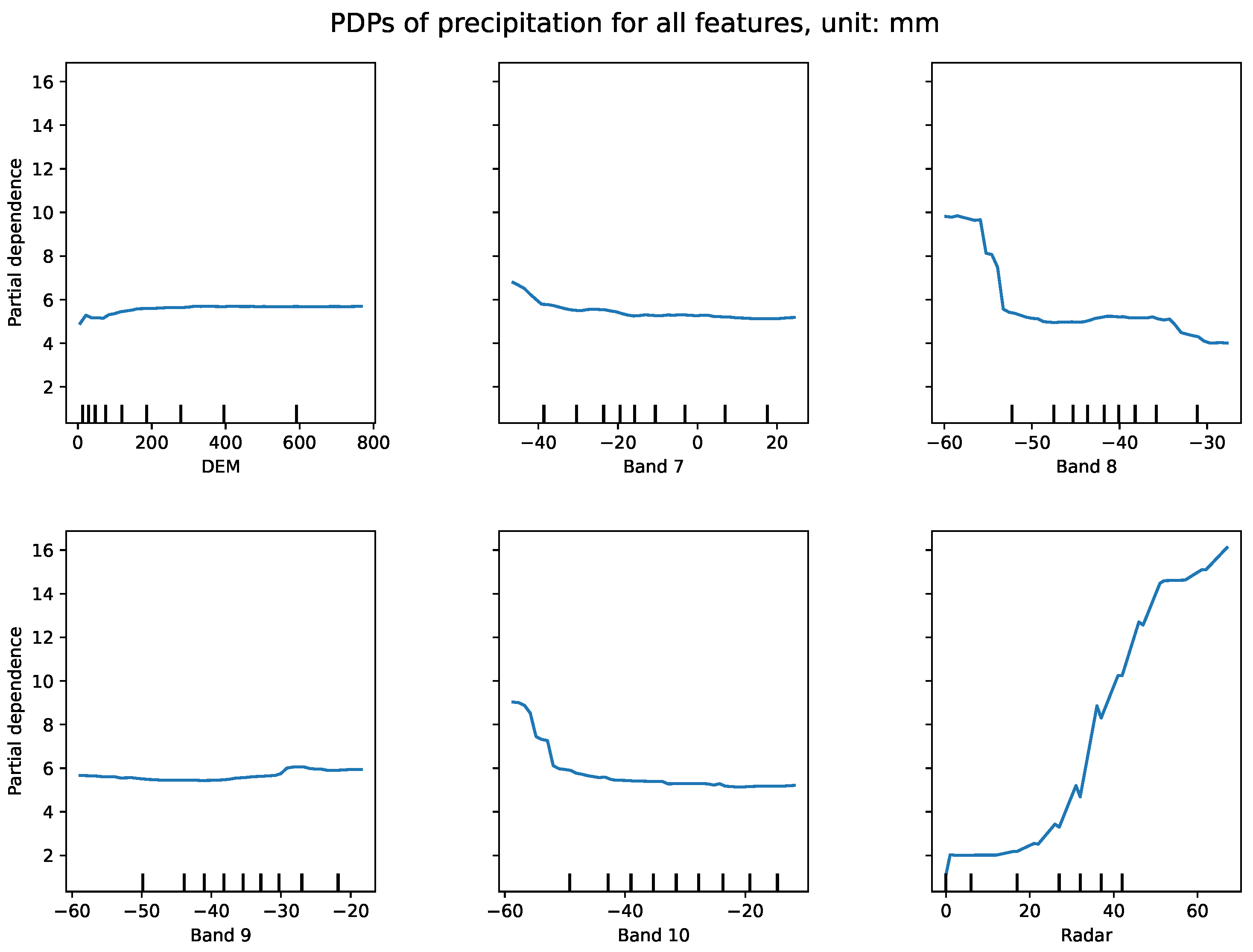
Figure 4.
PDP for six features at a resolution of 30 intervals. Precipitation rate shows the strongest dependence on radar echo, increasing as radar echo values rise. In contrast, the satellite feature exhibits a weaker influence. The resolution parameter refers to the number of equally spaced points along the x-axis, with higher resolution indicating a greater density of sample points within each interval.
The DEM data analysis reveals that most topography in this region lies below 800 meters elevation, indicating that terrain height within this range exerts no explicit influence on precipitation prediction. The distribution shows a concentration of radar data samples below 20 dBZ with relatively few samples exceeding 45 dBZ. Satellite data exhibits a more uniform distribution, which helps prevent model overfitting.
The PDPs clearly demonstrate that precipitation rate shows strong dependence on radar reflectivity (lower right panel) and exhibits an inverse relationship with satellite band 8 data (top right panel), where precipitation rates decrease as band 8 values increase. Radar data emerges as the dominant predictor with positive correlation to precipitation, consistent with operational forecasting practices that rely on radar data for QPE. Satellite band 10 data significantly influences precipitation predictions below -50 ∘C, displaying consistent negative correlation. Other satellite bands show varying degrees of influence on predictions, with band 9 demonstrating minimal impact on precipitation rate determination (bottom left panel).
Further examination reveals that precipitation prediction shows limited dependence on radar reflectivity below 20 dBZ, but this partial dependence increases dramatically when reflectivity exceeds 25 dBZ. This pattern confirms meteorological understanding that higher radar reflectivity values generally correspond to greater precipitation amounts. However, samples with high radar reflectivity values are comparatively scarce in the dataset. The following section provides detailed analysis of how this sample distribution affects prediction results.
3.4. Sample Distribution of Radar Reflectivity
Figure 5(a) presents a visualization of target radar reflectivity sample distribution. All sample points are divided into seven categories to demonstrate that the number of sample points in each category is relatively equal, avoiding bias toward any single category. The first category contains 3,322 sample points with radar reflectivity values between 0 and 12 dBZ. These points have an average actual precipitation of 1.070 mm as shown in Figure 5(a), while the model predicts an average of 0.755 mm for this category as shown in Figure 5(b). Similarly, the second category comprises 1,501 samples with reflectivity ranging from 12 to 22 dBZ, having an average actual precipitation of 1.895 mm, with the model predicting a median precipitation of 2.003 mm. Other categories follow the same interpretation pattern, revealing that when considering only single-source radar features, the model underestimates precipitation in low value ranges (0-22 dBZ) and overestimates precipitation in higher value ranges. This occurs because high radar value points with corresponding high precipitation constitute the majority in the sampling dataset, guiding the model toward overestimation. Therefore, the imbalanced data distribution significantly influences prediction accuracy. To verify this assumption, satellite data are incorporated as supplementary information for analysis, providing the model with additional features for improved predictions.
3.5. Sample Distribution of the Satellite Band 8 Data
Himawari-8 band 8 data is selected to analyze its sample distribution, as illustrated in Figure 6. This dataset is divided into nine categories, each containing approximately 1,600 sample points. The satellite data provides more nuanced distinctions between samples compared to radar data, offering additional information that helps generate more precise decision trees. When incorporating satellite data, the model underestimates rainfall amounts compared to ground truth measurements. This persistent underestimation likely stems from data imbalance in satellite data sampling, where sample points representing light or no rainfall dominate categories with brightness temperature above 0°C. This imbalance introduces bias toward lower precipitation predictions, providing opposite performance characteristics compared to radar analysis. The analysis thus far has examined radar and satellite features independently, without exploring how their interaction might influence precipitation estimations. While individual feature analyses provide valuable insights, they fail to capture the complex relationships between different data sources. To address this limitation, the following section investigates PDPs that demonstrate interactions between feature pairs, revealing how these variables jointly influence the model’s precipitation forecasts.
3.6. Interaction Between Two Features
Figure 7 explores the interaction effects between radar reflectivity and satellite band 8 data. The individual partial dependence of radar and band 8 are displayed above and left of the gridded plot, while the grid values represent the combined partial dependence between the two features. The grid values do not simply equal the sum of individual partial dependencies, confirming significant interaction effects between radar and satellite data that previous analysis overlooked. The PDP shows substantial variation along the horizontal axis (radar reflectivity) but minimal changes along the vertical axis (satellite data), indicating that radar reflectivity serves as the dominant predictor. This pattern reveals that with constant brightness temperature, increased radar reflectivity corresponds to higher precipitation predictions, while changes in satellite data have minimal impact when radar values remain fixed. Additionally, examination of the rightmost column (largest range of radar reflectivity) reveals that relatively higher brightness temperature values (yellow grids in the third and fourth rows) generate high partial dependence. This demonstrates that precipitation do not necessarily require the coldest brightness temperatures.
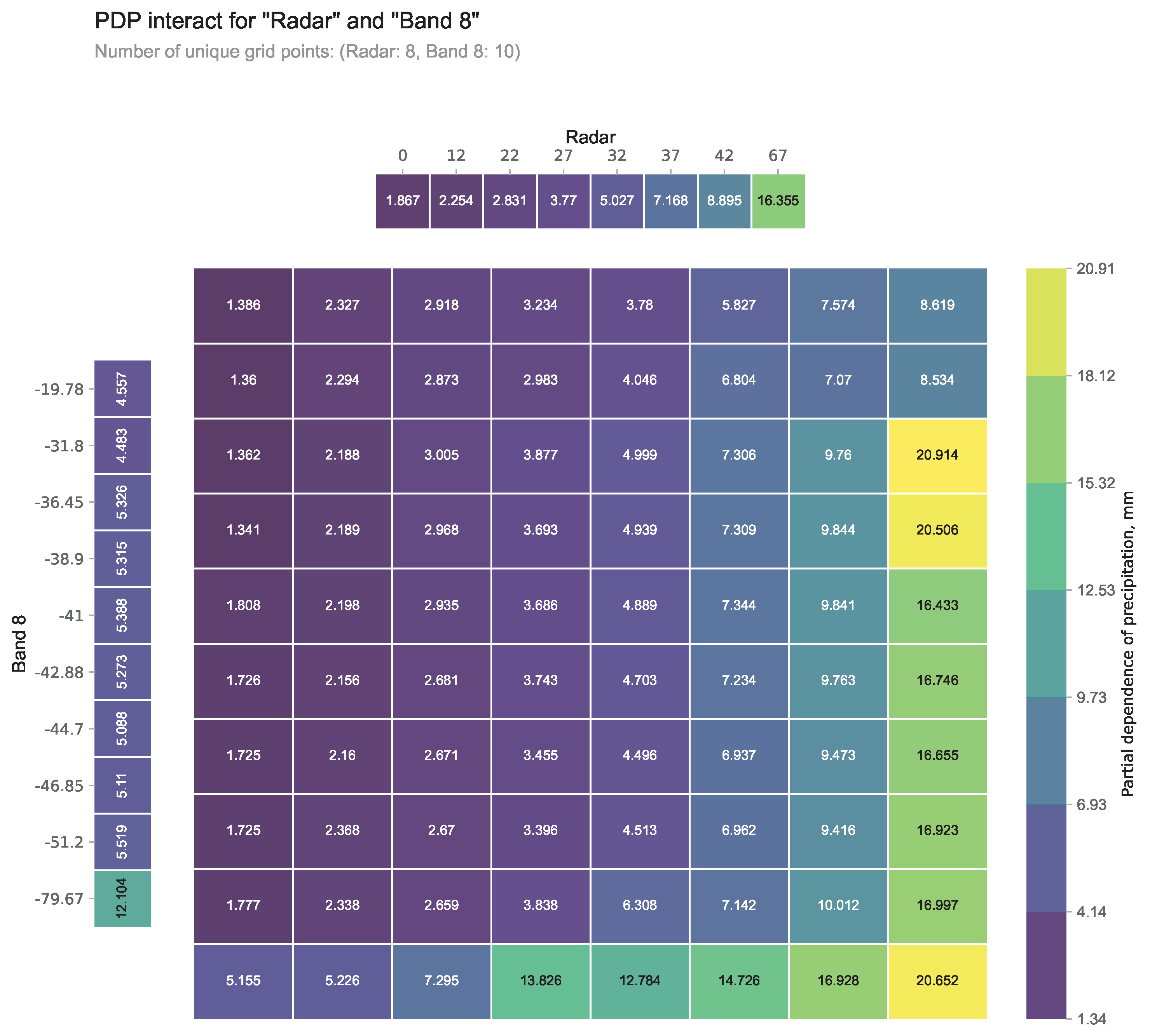
Figure 7.
2D PDP plot showing the interaction between radar and satellite band 8 features. The grid values indicate the combined partial dependence of precipitation estimates on both features simultaneously. Higher values (yellow regions) reflect stronger influence on precipitation predictions, while lower values (purple regions) indicate weaker dependence. The marginal plots along the upper and left edges show the individual partial dependence for radar and satellite band 8, respectively. Each grid cell represents a category corresponding to those shown in Figure 5 and 6.
To gain deeper insight into these feature interactions, Figure 8 presents a three-dimensional PDP with 30 unique grid points per feature. This visualization exposes details not apparent in the two-dimensional representation. The 3D plot demonstrates contrasting precipitation prediction patterns based on radar reflectivity thresholds. For values below 30 dBZ, precipitation partial dependence increases as band 8 brightness temperature decreases. However, for radar reflectivity exceeding 50 dBZ, predictions show minimal dependence on satellite data. The highest partial dependence values occur where radar reflectivity exceeds 40 dBZ, consistent with patterns observed in Figure 7. Most notably, Figure 8 reveals an abrupt change in partial dependence at approximately 50 dBZ, indicating that RuleFit effectively categorizes precipitation into two distinct types based on radar reflectivity thresholds. This classification aligns with meteorological practice of distinguishing between convective precipitation (heavy rain) and stratiform cloud precipitation (light rain) [6]. Meteorologists typically estimate these precipitation types separately using different reflectivity-rainfall relationships [8]. The fact that RuleFit independently developed a similar classification approach to that used by meteorologists enhances the credibility of its predictions and suggests the model has captured physically meaningful patterns rather than statistical correlations alone.
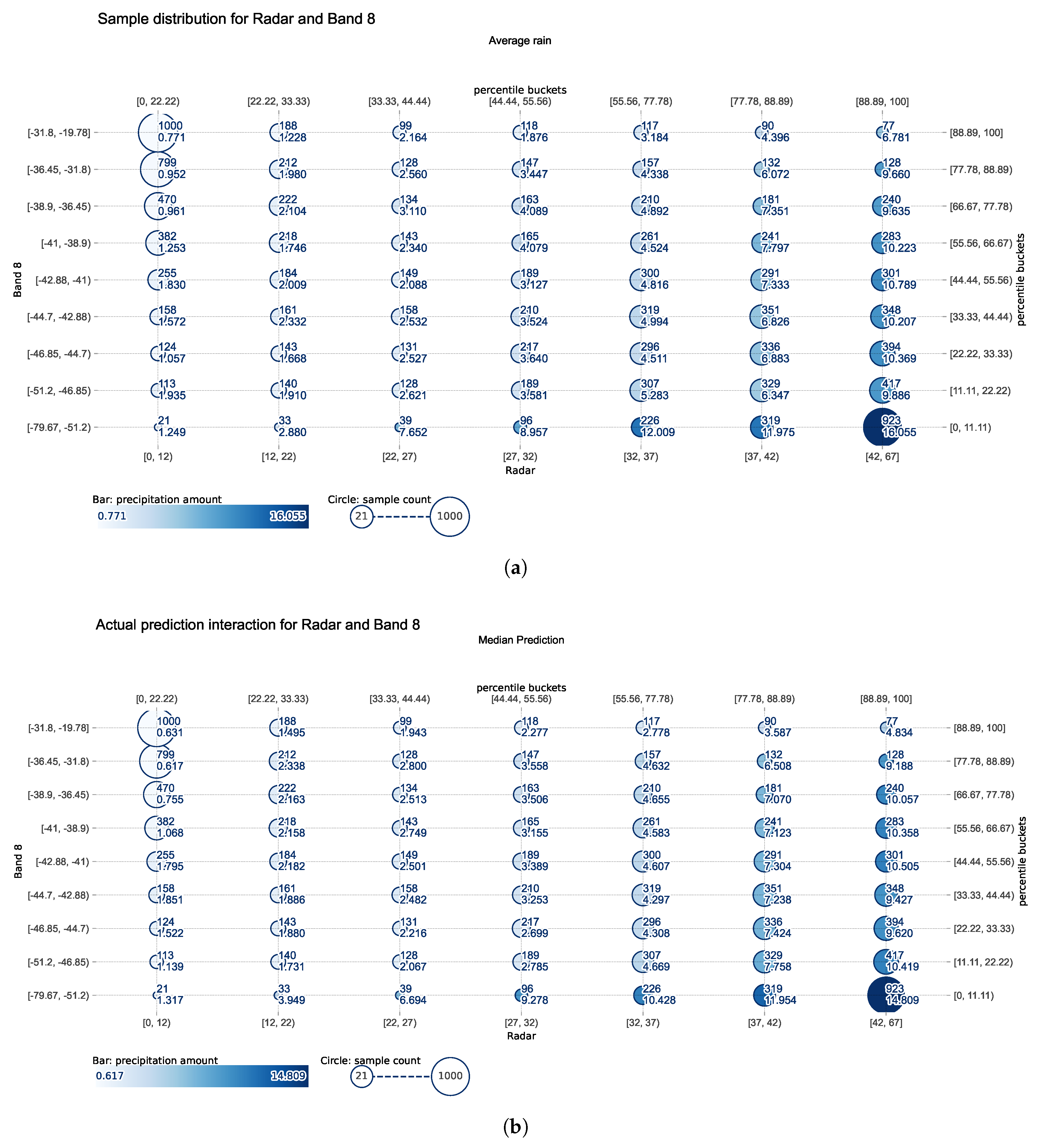
3.7. Joint Sample Distribution of the Radar Data and Satellite Band 8 Data
As previously discussed, the joint sample distribution’s effect on precipitation partial dependence across two key features is shown in Figure 9. The visualization combines seven categories of radar data with nine categories of satellite band 8 data, creating a comprehensive 63-category joint distribution. Circle size represents the sample count in each category, ranging from 21 to 1,000 points, while color intensity indicates the average precipitation amount. Each circle displays two values: the upper right shows the sample count, and the bottom right shows the average precipitation for that category. Comparing predicted versus target precipitation reveals strong alignment across most categories. The first two columns of samples(light rain) in the prediction plot closely match the target values, and most samples in the final column(heavy rain) also demonstrate high consistency with actual measurements. Band 8 data plays an important role in determining whether the model underestimates or overestimates precipitation. For example, the first row in Figure 9(b) shows lower values than those in Figure 9(a), revealing underestimation when satellite brightness temperature is relatively higher than other samples. The last row in both panels presents an opposite pattern, demonstrating that when brightness temperature conditions are sufficiently cool, the model tends to overestimate precipitation in low radar reflectivity points (lower than 32 dBZ), while still providing underestimation for high-value sample points (final three columns in the last row). The joint analysis of these complementary data sources captures precipitation patterns more accurately than either source alone, confirming the value of the multi-feature modeling approach and providing insights helpful for further research to correct estimation results of ML models.
4. Discussion
In the field of QPE, traditional Z–R relationships based on fixed empirical formulas often fail to capture the spatial and temporal variability inherent in precipitation systems. While previous ML approaches have primarily focused on improving accuracy, they have generally paid less attention to whether the decision-making processes behind their predictions are physically meaningful [14,16,18]. The method proposed in this paper leverages multisource data through data-driven techniques to more accurately characterize the nonlinear relationships present in precipitation events. Specifically, this paper explores how RuleFit, an interpretable ML algorithm, can uncover physically meaningful insights into QPE.
RuleFit effectively addresses the challenge of modeling nonlinear relationships between diverse remote sensing data and precipitation by automatically incorporating feature interactions into linear models. It demonstrates a compelling solution to the longstanding trade-off between predictive accuracy and model interpretability in QPE. The results show that RuleFit achieves competitive performance metrics while maintaining full transparency in its decision-making process.With correlation coefficients of 0.5416 and 0.6298 in the original and resampled datasets respectively, RuleFit consistently ranks among the top three performers across all evaluation scenarios. This performance is particularly noteworthy given that the model generates explicit rules that can be directly interpreted by meteorologists, unlike black-box approaches such as neural networks or ensemble methods.The precipitation estimation case reveals RuleFit’s superior ability to control precipitation distribution patterns, avoiding the spurious light precipitation artifacts that appear in other ML models while maintaining realistic spatial gradients. This spatial coherence suggests that RuleFit’s rule-based structure inherently captures meaningful meteorological relationships rather than exploiting statistical artifacts in the training data.
Additionally, the model-agnostic PDP method provides intuitive visualization of how individual features influence predictions. However, PDPs have a significant limitation in their assumption of feature independence. When analyzing radar and satellite data for precipitation prediction, PDPs assume that radar reflectivity values are uncorrelated with satellite measurements, which does not reflect reality. For instance, when calculating partial dependence at high radar reflectivity values like 50 dBZ, the method averages across the marginal distribution of satellite data, potentially including unrealistically high brightness temperatures exceeding 30°C that would rarely occur alongside such radar measurements. In actual atmospheric conditions, these features are strongly correlated, and the probability of such combinations would be extremely low. To address this limitation, alternative model-agnostic approaches such as Accumulated Local Effect plots offer a promising solution, as they work with conditional rather than marginal distributions, better preserving the natural relationships between correlated meteorological variables and providing more meteorologically consistent interpretations of model behavior.
Meanwhile, another important limitation with all ML methods lies in that, they train the data in the form of sample point, which lose the spatial and temporal correlation of each precipitation events. Even adding DEM data introduces the influence of topography, it still breaks the spatial interaction of neighboring points. In the future research, a better method should be designed that considers both historical temporal evolution of precipitation and spatial dependency in specific timestep. In computer vision field, spatial-temporal sequence prediction architecture could fill the gap and generative model such as Generative Adversarial Network(GAN) and diffusion models will help solve the blurry image problem of traditional regressive models, generate more authentic precipitation distribution.
On the other hand, the basic principles governing radar observation exert a profound influence on the accuracy and interpretation of QPE. Radar fundamentally measures the backscattering ability of hydrometeors (such as raindrops, snowflakes, and hail) to the radar beam. Consequently, the precision of QPE is highly contingent upon various factors, including precipitation type, particle size distribution, and geographical region. It is critical to acknowledge that radar exhibits distinctly different response characteristics to various hydrometeor phases, including liquid water droplets, ice crystals, snowflakes, and hail. For instance, the presence of a “Bright Band” (melting layer) often leads to an anomalous increase in reflectivity, whereas ice-phase precipitation generally yields lower reflectivity values [41]. While our study focuses on the flood season in China from May to September, a period predominantly characterized by warm rain events, the model’s capacity to effectively differentiate and process precipitation of varying phases remains an area requiring further investigation and validation. This aspect highlights a potential limitation in applying models trained on specific precipitation regimes to broader meteorological contexts without further scrutiny.
For operational meteorological services, RuleFit offers several practical advantages that extend beyond raw predictive performance. The model’s interpretability facilitates easier integration into existing forecasting workflows, as meteorologists can understand and verify the reasoning behind precipitation estimates. This transparency is crucial for building confidence in automated precipitation products and enables forecasters to make informed decisions about when to override model outputs based on local knowledge or additional observational evidence.
The success of RuleFit in precipitation estimation suggests several promising research directions. Future work could explore the integration of RuleFit with ensemble methods to combine the interpretability of rule-based models with the robustness of ensemble approaches. Additionally, the rule-based framework could be extended to incorporate temporal dependencies more explicitly, potentially improving prediction accuracy for precipitation events with strong temporal correlation. Apart from precipitation, when it comes to meteorological events that have not been thoroughly investigated, such as tornado, hail, squall line, hurricane, Rulefit shows great potential to disclose the new insights that meteorologist may neglect.
5. Conclusions
This paper collects a comprehensive multisource dataset combining radar reflectivity, rain gauge data, DEM data, and Himawari-8 satellite data for QPE tasks, then applies RuleFit along with six baseline algorithms to model complex nonlinear relationships. RuleFit generates interpretable decision rules and sparse linear models with clear importance rankings, offering greater transparency than other methods. Additionally, based on the qualitative and quantitative comparisons presented in Section 3.1, RuleFit’s rule-based output effectively estimates precipitation while simultaneously classifying precipitation types through context-specific rules. This approach demonstrates strong physical meaningfulness and interpretability, as illustrated in Tables 5 and 6.
PDP analysis confirms radar reflectivity’s dominant role in precipitation estimation, with feature interactions revealing highest precipitation rates when reflectivity is high and brightness temperature is low. The three-dimensional analysis demonstrates RuleFit’s ability to naturally classify input features rather than merely fitting them. This classification aligns with meteorological practices by categorizing precipitation levels and enabling tailored analyses of different precipitation events. Despite dataset imbalance favoring light rainfall samples, the resampling approach substantially improved precipitation rate predictions compared to direct use of original data distribution, confirming that resampling and multisource data enhance model generalization capabilities. Therefore, the interpretability methods presented can be applied to other complex meteorological events and provide new physical insights for researchers addressing natural disasters. Experts could also use their domain knowledge to correct model predictions, helping achieve physically plausible results.
Besides, several limitations require consideration for future research. The proposed method neglects spatial and temporal correlations within precipitation events. Furthermore, some RuleFit-generated rules contain feature interactions that contradict meteorological domain knowledge, potentially producing adverse effects on predictions. Further research on interpretable ML is needed to better serve meteorological applications.
References
- Marshall, J.S.; Palmer, W.M.K. THE DISTRIBUTION OF RAINDROPS WITH SIZE. Journal of Atmospheric Sciences 1948, 5, 165–166. [Google Scholar] [CrossRef]
- Ryzhkov, A.; Zhang, P.; Bukovčić, P.; Zhang, J.; Cocks, S. Polarimetric Radar Quantitative Precipitation Estimation. Remote Sensing 2022, Vol. 14, Page 1695 2022, 14, 1695. [Google Scholar] [CrossRef]
- Kim, T.J.; Kwon, H.H.; Kim, K.B. Calibration of the reflectivity-rainfall rate (Z-R) relationship using long-term radar reflectivity factor over the entire South Korea region in a Bayesian perspective. Journal of Hydrology 2021, 593, 125790. [Google Scholar] [CrossRef]
- Wu, W.; Zou, H.; Shan, J.; Wu, S. A Dynamical Z-R Relationship for Precipitation Estimation Based on Radar Echo-Top Height Classification. Advances in Meteorology 2018, 2018, 8202031. [Google Scholar] [CrossRef]
- Libertino, A.; Allamano, P.; Claps, P.; Cremonini, R.; Laio, F. Radar Estimation of Intense Rainfall Rates through Adaptive Calibration of the Z-R Relation. Atmosphere 2015, 6, 1559–1577. [Google Scholar] [CrossRef]
- Wang, G.; Liu, L.; Ding, Y. Improvement of radar quantitative precipitation estimation based on real-time adjustments to Z-R relationships and inverse distance weighting correction schemes. Advances in Atmospheric Sciences 2012, 29, 575–584. [Google Scholar] [CrossRef]
- Yin, Z.; Zhang, P. RADAR Rainfall Calibration by Using the Kalman Filter Method. Journal of Applied Meteorological Science 2005, 16, 213–219. [Google Scholar]
- Kim, T.J.; Kwon, H.H.; Kim, K.B. Calibration of the reflectivity-rainfall rate (Z-R) relationship using long-term radar reflectivity factor over the entire South Korea region in a Bayesian perspective. Journal of Hydrology 2021, 593, 125790. [Google Scholar] [CrossRef]
- Hirose, H.; Shige, S.; Yamamoto, M.K.; Higuchi, A. High Temporal Rainfall Estimations from Himawari-8 Multiband Observations Using the Random-Forest Machine-Learning Method. Journal of the Meteorological Society of Japan. Ser. II 2019, 97, 689–710. [Google Scholar] [CrossRef]
- Hassan, D.; Isaac, G.A.; Taylor, P.A.; Michelson, D. Optimizing Radar-Based Rainfall Estimation Using Machine Learning Models. Remote Sensing 2022, Vol. 14, Page 5188 2022, 14, 5188. [Google Scholar] [CrossRef]
- Liu, M.; Zuo, J.; Tan, J.; Liu, D. Comparing and Optimizing Four Machine Learning Approaches to Radar-Based Quantitative Precipitation Estimation. Remote Sensing 2024, Vol. 16, Page 4713 2024, 16, 4713. [Google Scholar] [CrossRef]
- Shin, K.; Song, J.J.; Bang, W.; Lee, G.W. Quantitative Precipitation Estimates Using Machine Learning Approaches with Operational Dual-Polarization Radar Data. Remote Sensing 2021, Vol. 13, Page 694 2021, 13, 694. [Google Scholar] [CrossRef]
- Mihuleţ, E.; Burcea, S.; Mihai, A.; Czibula, G. Enhancing the Performance of Quantitative Precipitation Estimation Using Ensemble of Machine Learning Models Applied on Weather Radar Data. Atmosphere 2023, Vol. 14, Page 182 2023, 14, 182. [Google Scholar] [CrossRef]
- Chen, H.; Chandrasekar, V.; Tan, H.; Cifelli, R. Rainfall Estimation From Ground Radar and TRMM Precipitation Radar Using Hybrid Deep Neural Networks. Geophysical Research Letters 2019, 46, 10669–10678. [Google Scholar] [CrossRef]
- Moraux, A.; Dewitte, S.; Cornelis, B.; Munteanu, A. A Deep Learning Multimodal Method for Precipitation Estimation. Remote Sensing 2021, Vol. 13, Page 3278 2021, 13, 3278. [Google Scholar] [CrossRef]
- Chen, H.; Chandrasekar, V.; Cifelli, R.; Xie, P. A Machine Learning System for Precipitation Estimation Using Satellite and Ground Radar Network Observations. IEEE Transactions on Geoscience and Remote Sensing 2020, 58, 982–994. [Google Scholar] [CrossRef]
- Wehbe, Y.; Temimi, M.; Adler, R.F. Enhancing Precipitation Estimates Through the Fusion of Weather Radar, Satellite Retrievals, and Surface Parameters. Remote Sensing 2020, Vol. 12, Page 1342 2020, 12, 1342. [Google Scholar] [CrossRef]
- Guarascio, M.; Folino, G.; Chiaravalloti, F.; Gabriele, S.; Procopio, A.; Sabatino, P. A Machine Learning Approach for Rainfall Estimation Integrating Heterogeneous Data Sources. IEEE Transactions on Geoscience and Remote Sensing 2022, 60. [Google Scholar] [CrossRef]
- Ribeiro, M.T.; Singh, S.; Guestrin, C. "Why Should I Trust You?": Explaining the Predictions of Any Classifier. In Proceedings of the Proceedings of the 22nd ACM SIGKDD International Conference on Knowledge Discovery and Data Mining, New York, NY, USA, 2016; KDD ’16, p. 1135–1144. [CrossRef]
- Lipton, Z.C. The Mythos of Model Interpretability. CoRR 2016, abs/1606.03490, [1606.03490].
- Rudin, C. Stop explaining black box machine learning models for high stakes decisions and use interpretable models instead. Nature Machine Intelligence 2019, 1, 206–215. [Google Scholar] [CrossRef]
- Lundberg, S.M.; Lee, S.I. A unified approach to interpreting model predictions In Proceedings of the Proceedings of the 31st International Conference on Neural Information Processing Systems, Red Hook, NY, USA, 2017; NIPS’17, p. 4768–4777.
- Wang, R.; Chu, H.; Liu, Q.; Chen, B.; Zhang, X.; Fan, X.; Wu, J.; Xu, K.; Jiang, F.; Chen, L. Application of Machine Learning Techniques to Improve Multi-Radar Mosaic Precipitation Estimates in Shanghai. Atmosphere 2023, Vol. 14, Page 1364 2023, 14, 1364. [Google Scholar] [CrossRef]
- Li, W.; Chen, H.; Han, L. Improving Explainability of Deep Learning for Polarimetric Radar Rainfall Estimation. Geophysical Research Letters 2024, 51, e2023GL107898. [Google Scholar] [CrossRef]
- Investigating Black-Box Model for Wind Power Forecasting Using Local Interpretable Model-Agnostic Explanations Algorithm. CSEE Journal of Power and Energy Systems 2025. [CrossRef]
- Daif, N.; Di Nunno, F.; Granata, F.; Difi, S.; Kisi, O.; Heddam, S.; Kim, S.; Adnan, R.M.; Zounemat-Kermani, M. Forecasting maximal and minimal air temperatures using explainable machine learning: Shapley additive explanation versus local interpretable model-agnostic explanations. Stochastic Environmental Research and Risk Assessment 2025, 39, 2551–2581. [Google Scholar] [CrossRef]
- Huang, F.; Zhang, Y.; Zhang, Y.; Nourani, V.; Li, Q.; Li, L.; Shangguan, W. Towards interpreting machine learning models for predicting soil moisture droughts. Environmental Research Letters 2023, 18, 074002. [Google Scholar] [CrossRef]
- Wang, Y.V.; Kim, S.H.; Lyu, G.; Lee, C.L.; Lee, G.; Min, K.H.; Kafatos, M.C. Relative Importance of Radar Variables for Nowcasting Heavy Rainfall: A Machine Learning Approach. IEEE Transactions on Geoscience and Remote Sensing 2023, 61. [Google Scholar] [CrossRef]
- McGovern, A.; Lagerquist, R.; Gagne, D.J.; Jergensen, G.E.; Elmore, K.L.; Homeyer, C.R.; Smith, T. Making the Black Box More Transparent: Understanding the Physical Implications of Machine Learning. Bulletin of the American Meteorological Society 2019, 100, 2175–2199. [Google Scholar] [CrossRef]
- Toms, B.A.; Barnes, E.A.; Ebert-Uphoff, I. Physically Interpretable Neural Networks for the Geosciences: Applications to Earth System Variability 2019.
- Salih, A.M.A.; Raisi-Estabragh, Z.; Galazzo, I.; Radeva, P.; Petersen, S.E.; Lekadir, K.; Menegaz, G. A Perspective on Explainable Artificial Intelligence Methods: SHAP and LIME. Advanced Intelligent Systems 2023, 7. [Google Scholar] [CrossRef]
- Garreau, D.; Luxburg, U. Explaining the explainer: A first theoretical analysis of LIME. In Proceedings of the Proceedings of the International Conference on Artificial Intelligence and Statistics (AISTATS). PMLR, 2020, pp. 1287–1296.
- Doumard, E.; Aligon, J.; Escriva, E.; Excoffier, J.B.; Monsarrat, P.; Soulé-Dupuy, C. A comparative study of additive local explanation methods based on feature influences. In Proceedings of the Proceedings of the 24th International Workshop on Design, Optimization, Languages, and Analytical Processing of Big Data (DOLAP). ACM, 2022, pp. 31–40.
- Hooshyar, D.; Yang, Y. Problems With SHAP and LIME in Interpretable AI for Education: A Comparative Study of Post-Hoc Explanations and Neural-Symbolic Rule Extraction. IEEE Access 2024, 12, 137472–137490. [Google Scholar] [CrossRef]
- Friedman, J.H.; Popescu, B.E. Predictive learning via rule ensembles. Annals of Applied Statistics 2008, 2, 916–954. [Google Scholar] [CrossRef]
- Quinlan, J.R. Induction of decision trees. Machine Learning 1986 1:1 1986, 1, 81–106. [Google Scholar] [CrossRef]
- Wang, L.; Zeng, X.; Fang, H.; Dou, L. A Rulefit Based Model for Driving Intention Prediction at Intersections. In Proceedings of the 2023 China Automation Congress (CAC); 2023; pp. 405–410. [Google Scholar] [CrossRef]
- Li, S.; Zhang, W.; Liang, B.; Huang, W.; Luo, C.; Zhu, Y.; Kou, K.I.; Ruan, G.; Liu, L.; Zhang, G.; et al. A Rulefit-based prognostic analysis using structured MRI report to select potential beneficiaries from induction chemotherapy in advanced nasopharyngeal carcinoma: A dual-centre study. Radiotherapy and Oncology 2023, 189, 109943. [Google Scholar] [CrossRef] [PubMed]
- Kato, H.; Hanada, H.; Takeuchi, I. Safe RuleFit: Learning Optimal Sparse Rule Model by Meta Safe Screening. IEEE Transactions on Pattern Analysis and Machine Intelligence 2023, 45, 2330–2343. [Google Scholar] [CrossRef] [PubMed]
- Shi, X.; Chen, Z.; Wang, H.; Yeung, D.Y.; Wong, W.k.; Woo, W.c. Convolutional LSTM Network: A Machine Learning Approach for Precipitation Nowcasting. In Proceedings of the Proceedings of the 28th International Conference on Neural Information Processing Systems - Volume 1, Cambridge, MA, USA, 2015; NIPS’15, pp. 802–810.
- Herzegh, P.; Jameson, A.R. Observing Precipitation through Dual-Polarization Radar Measurements. Bulletin of the American Meteorological Society 1992, 73, 1365–1374. [Google Scholar] [CrossRef]
Figure 1.
Data distribution and visualization in this study: (a) Geographic distribution of automatic weather stations across eastern China. (b) Sample composite radar reflectivity data. (c) Representative precipitation observations. (d) DEM representation showing topographical features. (e) Example of Himawari 8 satellite imagery from Band 7 with brightness temperature values in degrees Celsius. (f) Himawari 8 Band 8. (g) Himawari 8 Band 9. (h) Himawari 8 Band 10.

Figure 2.
Qualitative Performance on one of precipitation estimation case.
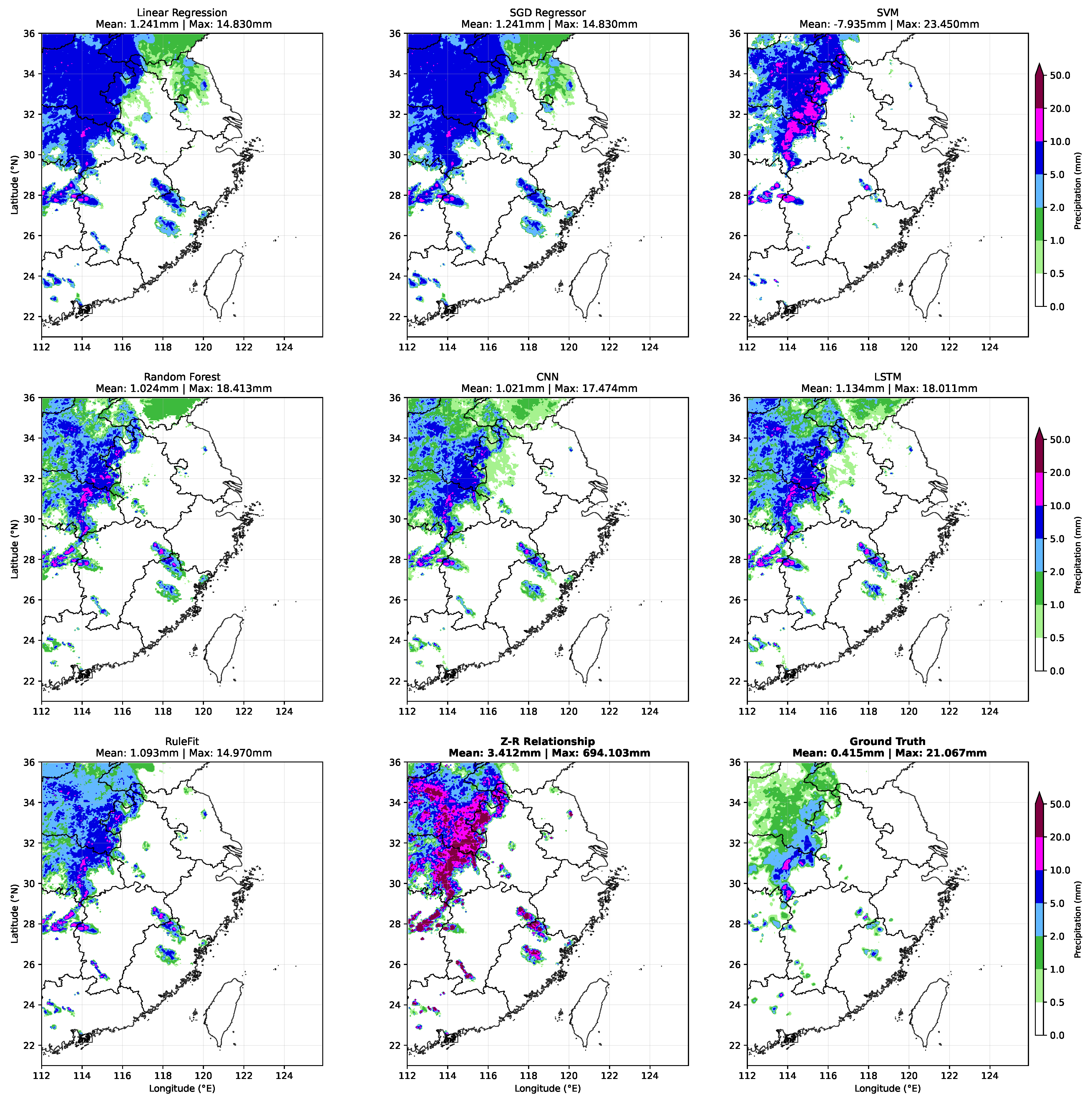
Figure 3.
One of a decision tree estimator illustrating how data at different sample points are separated by specific rules at each node. When the rules are met, the mean squared error (MSE) with labels is calculated, resulting in the number of suitable samples and the value of predicted precipitation rate indicated within the frames of the figure. Other sample points are evaluated against additional rules to determine their classification. When the pretrained parameters are loaded, RuleFit will generate the same threshold values. The tree shown is just a single tree from the Rulefit ensembles and used to help provide an interpretable explanation of how RuleFit makes its decisions.
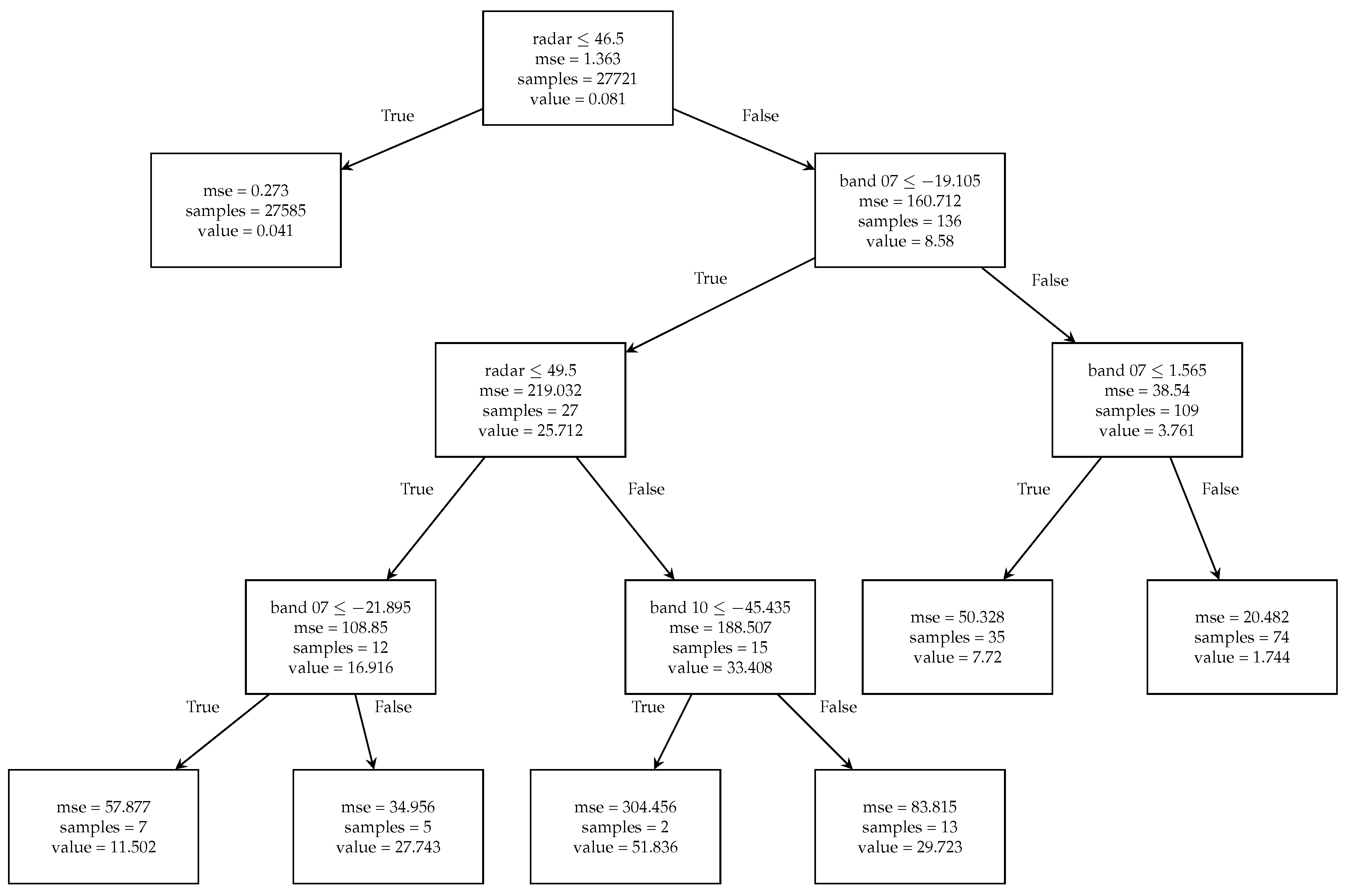
Figure 5.
Comparison of observed and predicted precipitation for radar feature: (a) Distribution of radar reflectivity values with corresponding ground truth average precipitation; (b) Rulefit model predictions for the same radar reflectivity ranges. Bar heights represent the number of sample points in each category, with numerical labels showing exact counts. Line graphs display the average precipitation amount within each category, enabling direct comparison between observed (panel a) and predicted (panel b) values.
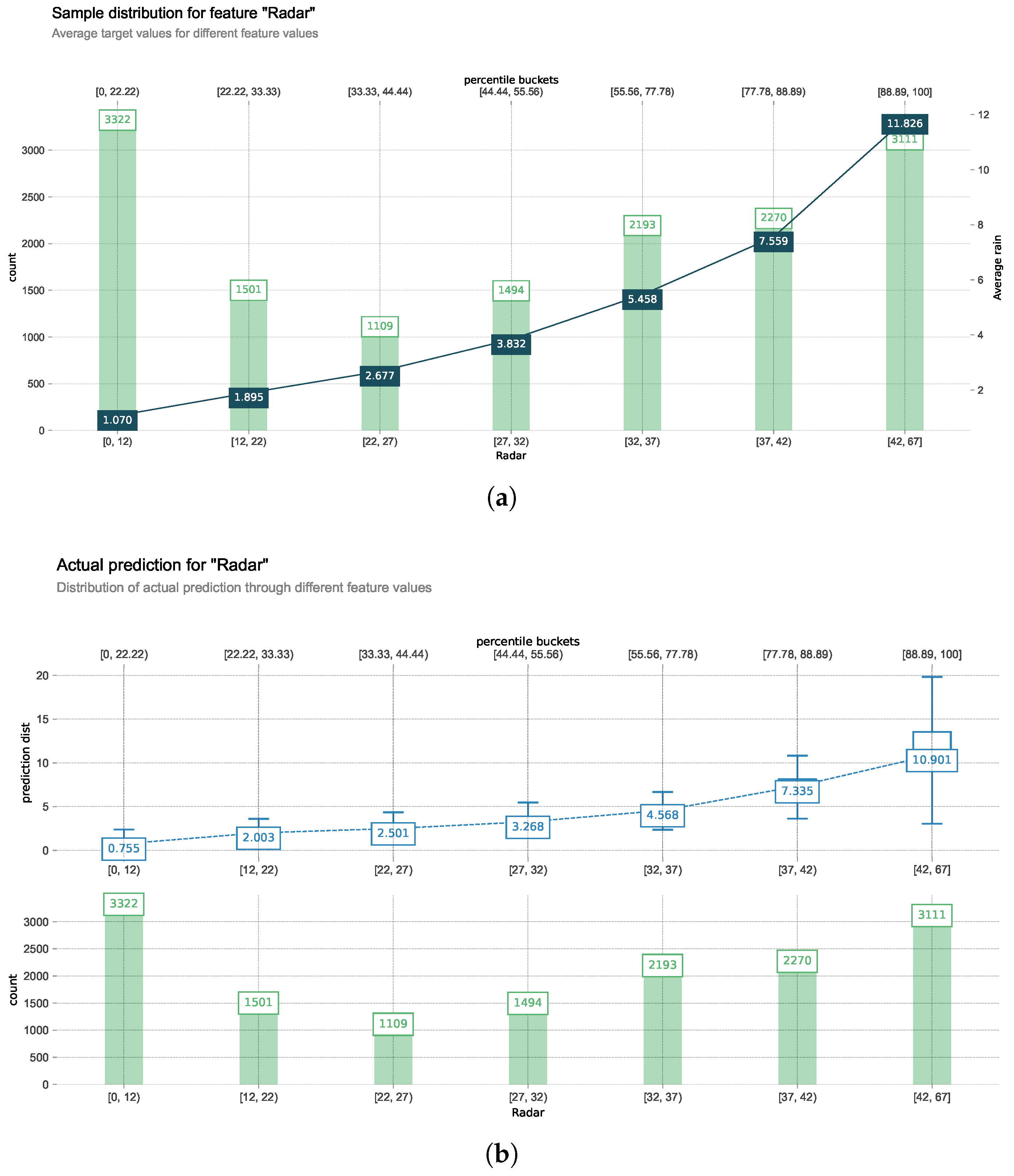
Figure 6.
Comparison of observed and predicted precipitation for satellite band 8: (a) Distribution of satellite band 8 data with corresponding ground truth average precipitation; (b) Rulefit model predictions for the same satellite data value ranges. Samples are grouped into 10 categories based on satellite band 8 values. Bar heights represent the number of sample points in each category, with numerical labels showing exact counts. Line graphs display the average precipitation rate within each category, enabling direct comparison between observed (panel a) and predicted (panel b) values.
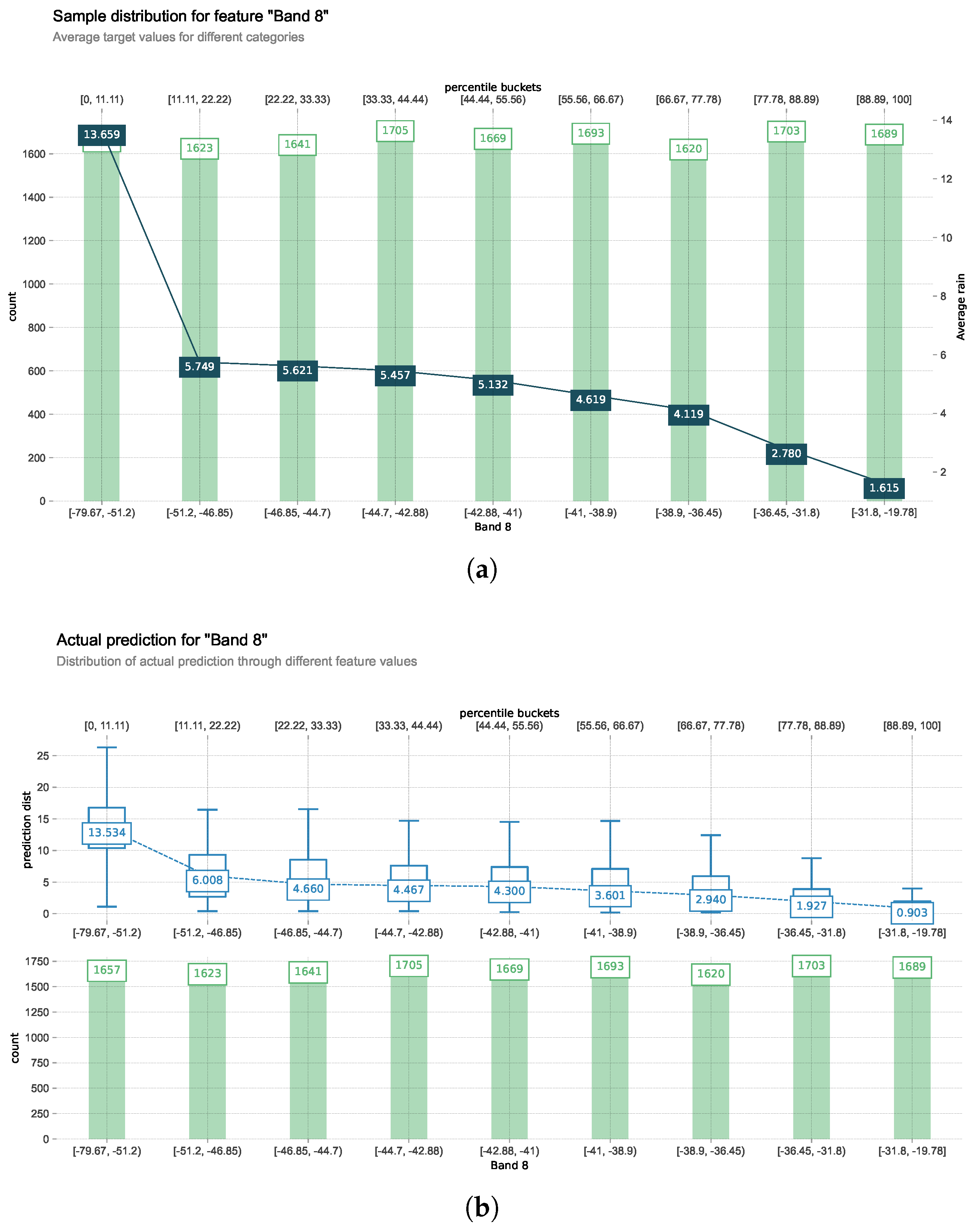
Figure 8.
3D PDP plot for radar and satellite band 8 data. The partial dependence pattern mirrors that of the 2D plot, with a clear separation dividing sample points into two categories: heavy rain and light rain.
Figure 8.
3D PDP plot for radar and satellite band 8 data. The partial dependence pattern mirrors that of the 2D plot, with a clear separation dividing sample points into two categories: heavy rain and light rain.
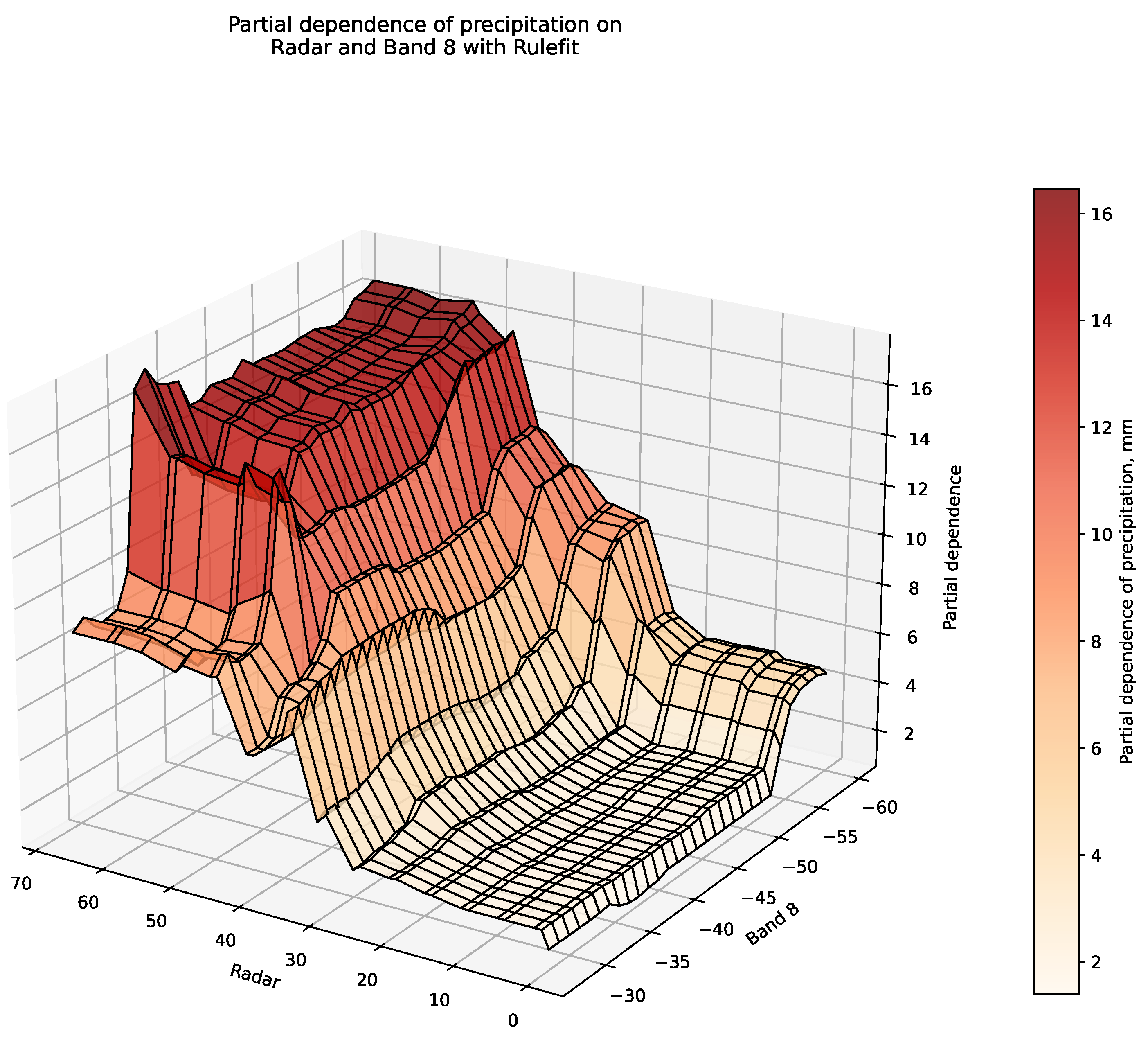
Figure 9.
Joint sample distribution of different data: (a) Radar reflectivity and satellite band 07 data plotted with corresponding target precipitation at each sample point. (b) Distribution of predicted precipitation across different sample categories. Circle size indicates the number of samples per category, while color intensity and values represent the mean precipitation rate within each category.
Disclaimer/Publisher’s Note: The statements, opinions and data contained in all publications are solely those of the individual author(s) and contributor(s) and not of MDPI and/or the editor(s). MDPI and/or the editor(s) disclaim responsibility for any injury to people or property resulting from any ideas, methods, instructions or products referred to in the content. |
© 2025 by the authors. Licensee MDPI, Basel, Switzerland. This article is an open access article distributed under the terms and conditions of the Creative Commons Attribution (CC BY) license (http://creativecommons.org/licenses/by/4.0/).
Copyright: This open access article is published under a Creative Commons CC BY 4.0 license, which permit the free download, distribution, and reuse, provided that the author and preprint are cited in any reuse.


