Analysis of Trail Networks and Routes Optimization in Mountain Areas: New Tools in GIS Environment

1. Introduction

Graph theory has long been used in quantitative geography for the spatial analysis of multiple phenomena [1,2], and even today, within the so-called geospatial sciences, algorithms derived from it are widely used for their capacity to detect and synthesize the spatial structure and relationships of multiple phenomena in various disciplines (transportation, planning, ecology, geosciences, disaster studies, etc.) [3,4]. The spread of digital cartography and the development of Geographic Information Systems (GIS) have contributed significantly to the realization of increasingly sophisticated applications of the concepts and methods of graph theory, thus providing increasingly effective tools for the analysis, modeling, and management of spatial structures.

A relatively little explored context for spatial structures, and network analysis in particular, is the study of hiking trail networks. In this field the study of the topology of the networks serves two purposes: the identification of critical spots for maintenance and the setup of the topology for further analysis, such as path optimization.

This article proposes an automatic process for analyzing and improving mountain hiking routes.

These tools are tested in Trentino, an Alpine region particularly rich in this type of itineraries.

1.1. Trail Network in the Trentino Region

The Italian area of Trentino, corresponding to the Autonomous Province of Trento (PAT), is situated in the northeastern Alps and is primarily covered by mountains and woods. It provides a wealth of outdoor activities, including hiking, mountain biking, mountaineering and winter sports.

An accurate representation of its morphology and the evolution of its forest landscapes has recently been achieved within the Trentinoland project. It used historical maps [5,6,7,8] and aerial photos [9] to create a comprehensive dataset detailing the landscape and ecological development of the area.

The Provincial Environment and Territory Information System (Sistema Informativo Ambiente e Territorio, SIAT) of the PAT provides a digital map of the Trentino mountain trail network (Figure 1 and Figure 2) [10].

Although the primary purpose of this map is to guide hikers using GPX-formatted trails in navigation apps, the digital version of the map allows for the incorporation of this data into environmental models within a GIS.

In particular, it is possible to use this map for the analysis of the network topology and for determining optimal routes.

In this study the topology analysis of the Trentino mountain trail network has been carried out following the methodology applied by Kołodziejczyk [11] and Taczanowska et al. [12], with particular respect to its connectivity and redundancy. Moreover, the network connectivity and centrality are evaluated also with respect to the alpine huts [13].

1.2. Network Analysis for Trail Networks

Trail networks managers can investigate the network connectivity and find some important components, including the sections (arcs) that make up the so-called bridges, or the linking elements between various subnets that would otherwise be isolated, by using network analysis tools. Because of their relative significance, these arches need to be protected and maintained with greater care.

Trail networks researches are mostly focused on the optimal configuration features to design trail paths and spatial distribution of their facilities. Kolkos et al. [14] described the strategic design and ranking of trail paths using the multi-criteria decision-making (MCDM) VIKOR method. Tomczyk and Ewertowski [15] described a framework combining a GIS and the regression tree analysis to optimize the location of new recreational trails with the application to the Gorce National Park in the south of Poland. Snyder et al. [16] applied Cost Path algorithm in a GIS environment to plan recreational trail locations for all-terrain vehicles (ATVs), taking into account environmental factors and rider preferences for trail attributes.

Other studies report procedures to describe a network trail and its use. For example, Chiou et al. [17] applied dynamic segmentation and network analysis techniques to collect trail routes data and generate travel time and energy consumption information in a forest recreational area in central Taiwan Island.

1.3. Path Optimization for Hiking Trail Networks

The second part of the paper presents an original procedure to evaluate costs, such as travel time and altitude difference, which can be used instead of the usual planimetric distance to evaluate optimal routes. While trail routes optimization is not new and the possibility of evaluating hiking time as a function of the slope of the trail is well known, in the application presented in this paper they are combined in a GIS framework. It is therefore possible to integrate the automatic evaluation of hiking times with all the other procedures available in a GIS environment. In particular, the combination of the new procedure for the hiking time assessment with the network analysis capability in a GIS provides a powerful tool for path optimization.

This approach has already been partially applied to identify and optimize itineraries for Literary Tourism [18] and here it is presented in a more detailed and complete way.

This procedure for the hiking time evaluation and its use as cost for path optimization has been made fully automatic using a Python script for GRASS GIS which is available in a public GitHub repository.

2. Materials and Methods

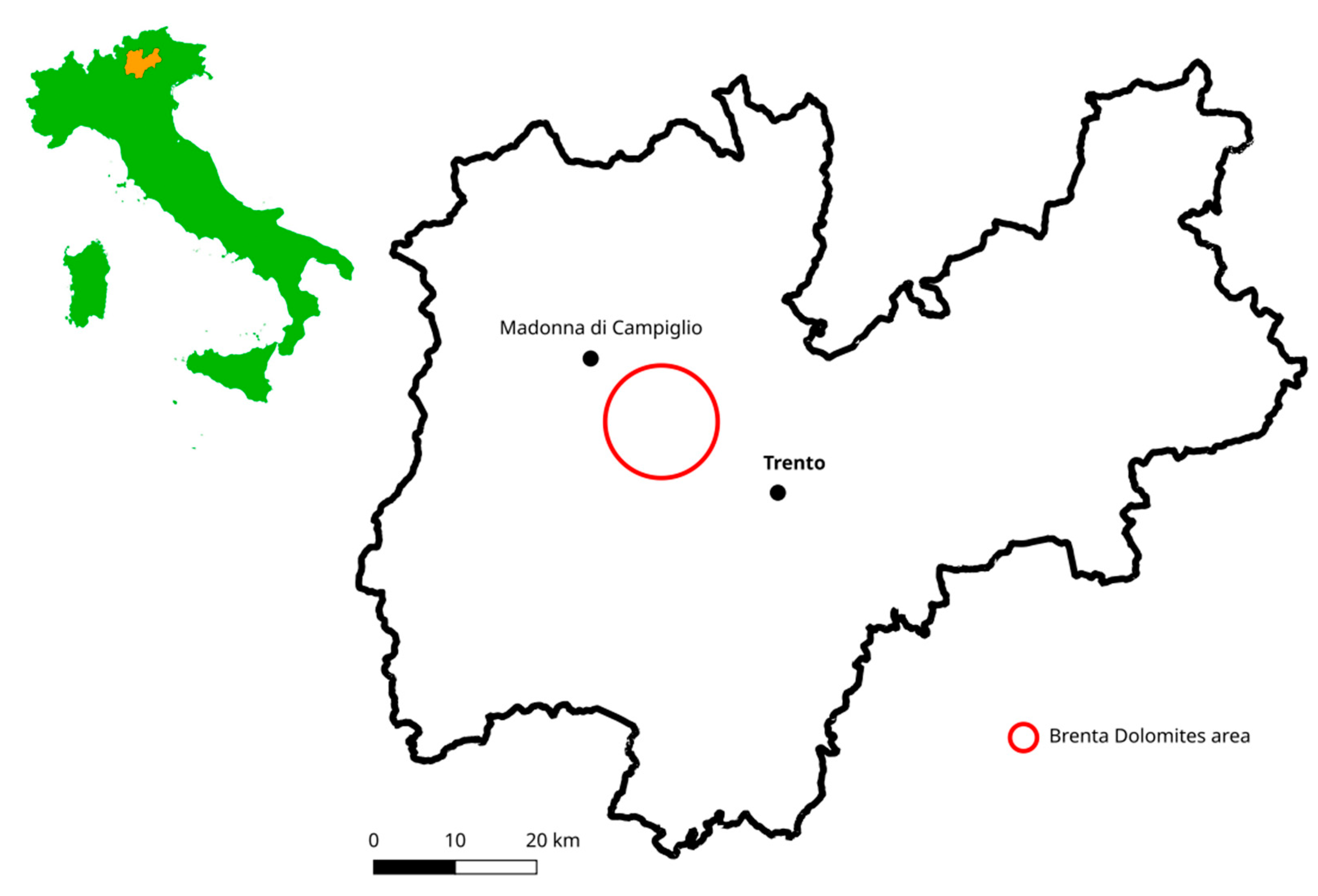
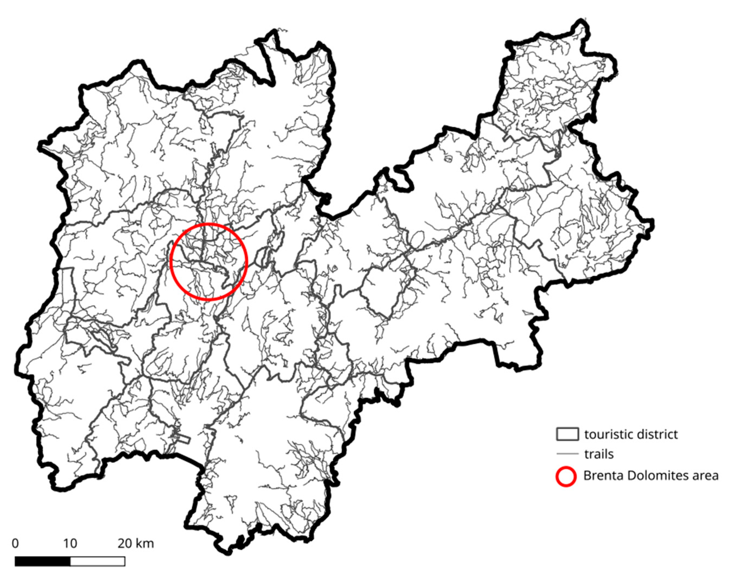
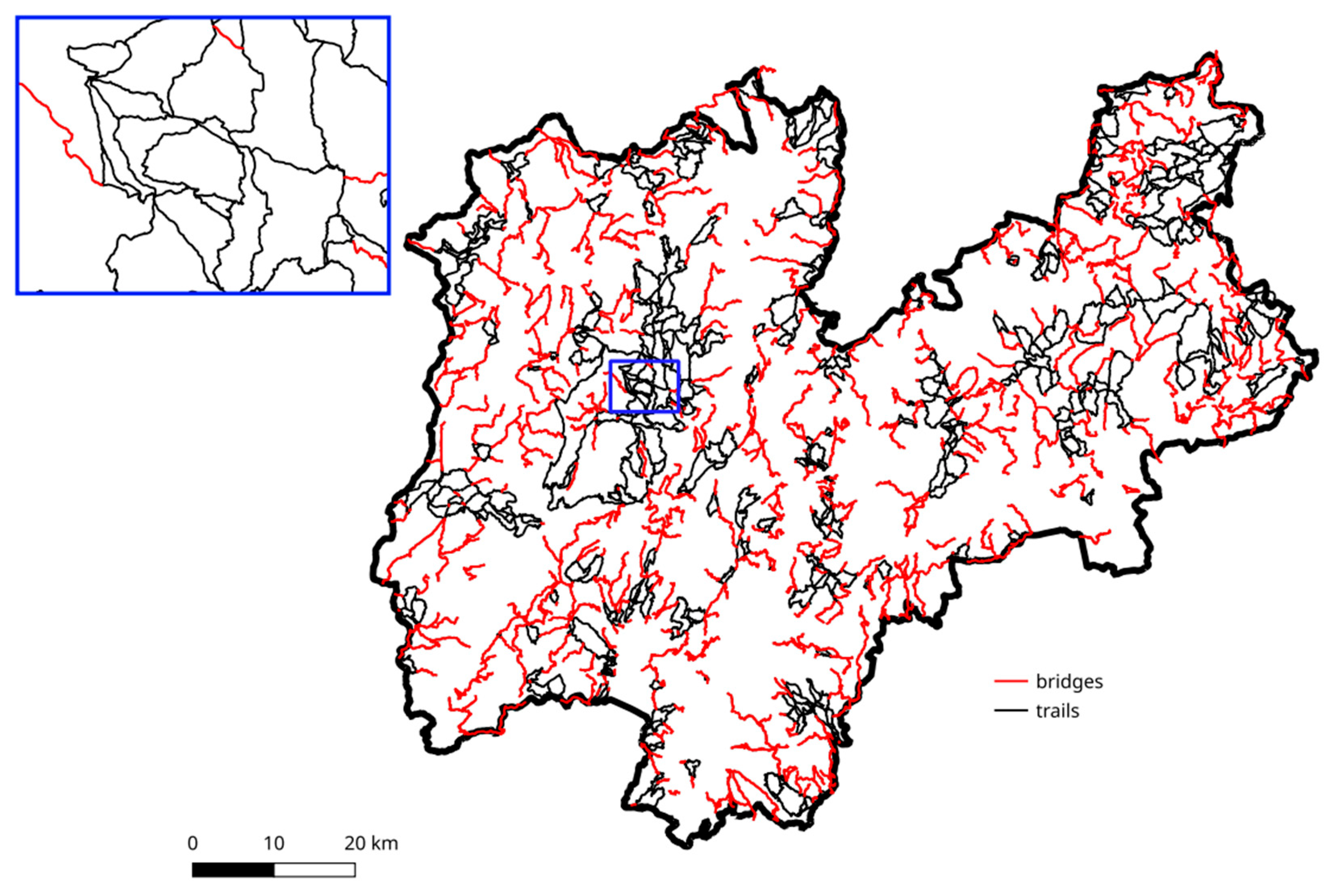
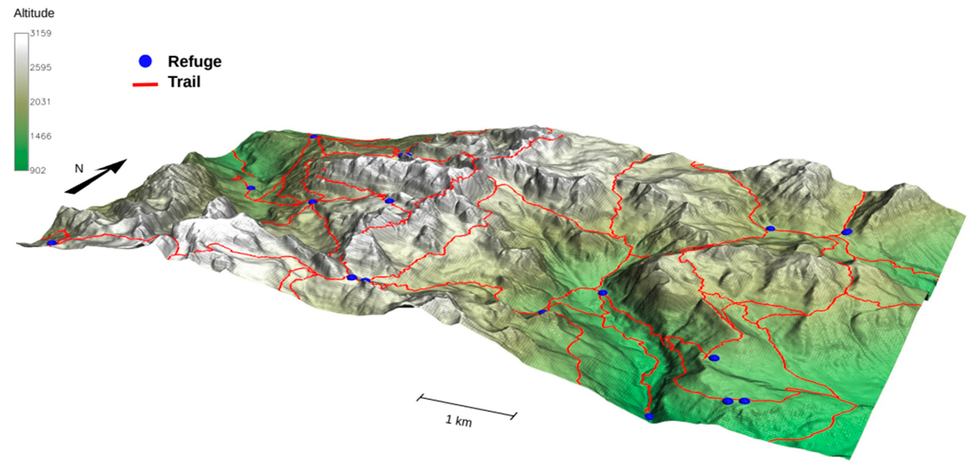
2.1. Study Area

With an elevation ranging from 64 m.a.s.l. (Valle del Sarca) to 3769 m.a.s.l. (Monte Cevedale), the Trentino region spans around 6200 km2, the majority of which is covered by woods.

The trail network [19] includes 866 alpine trails, 144 equipped alpine trails (with fixed cables, stemples, ladders and bridges) and 69 vie ferrate (fixed-rope routes) (Figure 2 and Table 1).

The PAT [10] trail vector map, which was last updated in 2021, is available in ESRI Shape file (SHP) format with a nominal scale of 1: 10,000.

The map of the alpine refuges is also a SHP file and available on the Portale Geocartografico Trentino [13]. Refuges are represented by points and their attributes include the refuge name, its unique identifier code, elevation, type (Rifugio - refuge, rifugio alpino - alpine refuge, or rifugio escursionistico - hiking refuge) and date of last update. The map has a nominal scale of 1: 10 000.

The Digital Terrain Model (DTM), which is accessible on the Portale Geocartografico Trentino [20], has been used to assess elevation, elevation changes, and slope at a resolution of 10 m.

All the maps are available under the CC0 1.0 Universal (CC0 1.0) Public Domain Dedication license with ETRS89/UTM32N (EPSG 25832) datum.

GRASS GIS 8.4 [21], a Free and Open Source GIS that is frequently used for geospatial research [22] and education [23], has been utilized for map maintenance and network analysis. GRASS GIS offers sixteen modules for network administration and analysis. Routing algorithms in GRASS are based on the Directed Graph Library (DGLib) [24].

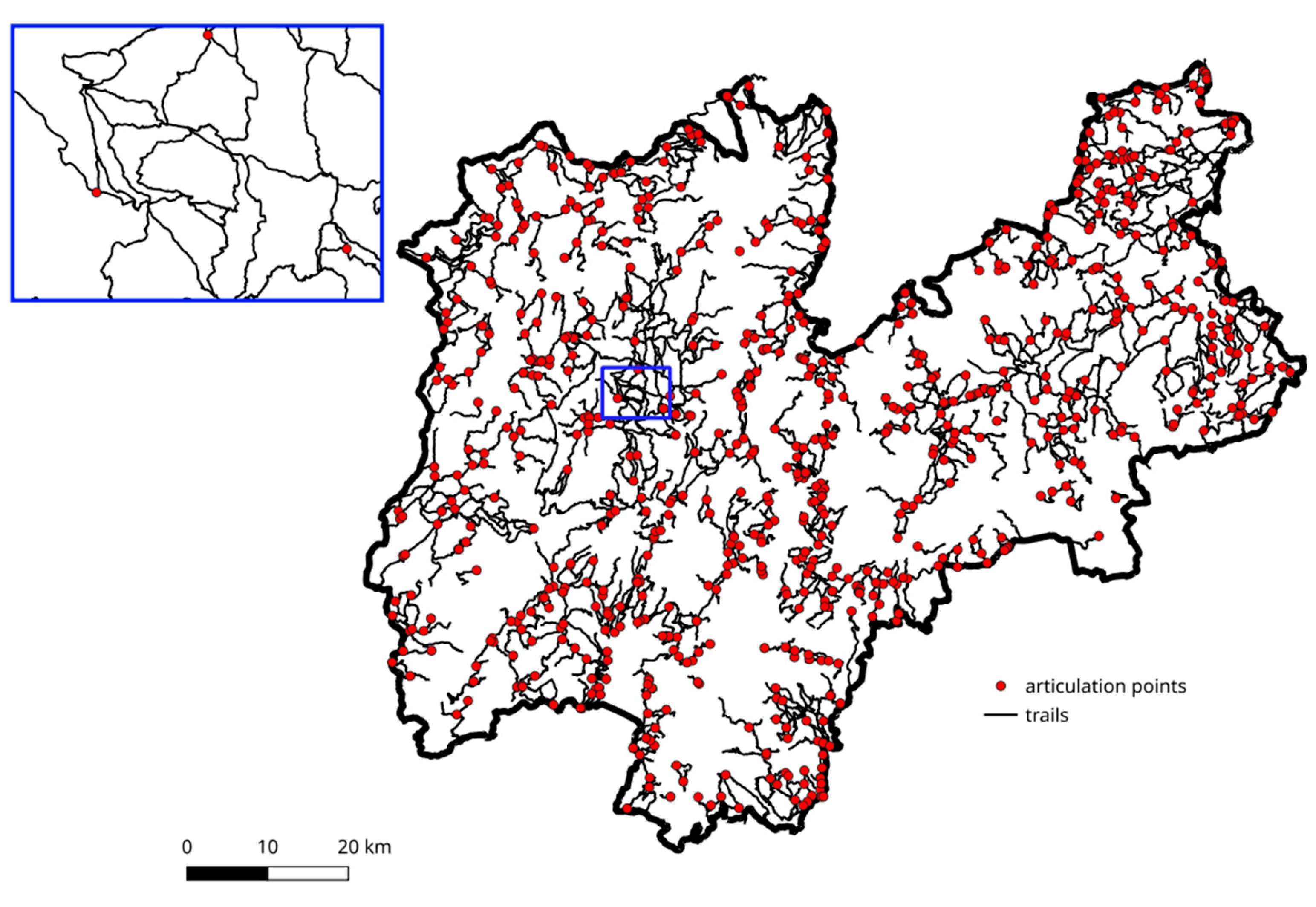
2.2. Topological Analysis of the Trail Network

The trail network is represented by a collection of nodes and arcs that show their relationships in order to determine the best routes. Therefore, the possible paths between the nodes and their features can be evaluated.

The original vector map, in ESRI Shape format, does not provide the network topology, which must therefore be created in a pre-processing step during the acquisition phase in a GIS system. Single trails are shown on the map as lines; shared sections between trails are shown as either overlapping segments or closely spaced but distinct lines. Additionally, nodes do not match trail intersections. To use there trails for network analysis, the map must be pre-processed to remove duplicate parts and break the path lines at intersections (Figure 3).

The majority of the issues were resolved by using automatic topology correction tools, which eliminated 163 duplicate lines and added 1625 nodes at the intersections. However, in certain situations, especially when some trails intersected multiple times over a short distance, manual intervention was required.

Alpine refuges, points of interest for hikers, have been incorporated into the route network ss nodes. In order to determine the best routes, each node has been given a normal residency duration, which can be utilized as the node’s “crossing” cost.

2.3. Global Connectivity Evaluation

Graph theory [25] and connectivity indices for network analysis [1,26] have been used to assess global connectedness.

Given the number of edges e, the number of nodes n and the number of isolated subgraphs p, it possible to define:

• $\mathsf{\mu }=\mathrm{e}-\mathrm{n}+\mathrm{p}$ number of cycles
• $\mathsf{\alpha }=\mathsf{\mu }/(2\mathrm{n}-5)$ which compares a graph’s number of cycles with the maximum number of cycles that could exist. A network with great redundancy and connectivity is indicated by high index values;
• $\mathsf{\beta }=\mathrm{e}/\mathrm{n}$ which measures a graph’s degree of connectedness by dividing its number of edges (e) by its number of nodes (n). For simple networks and trees, the value of β is less than 1, for a linked network with a single cycle, it is 1, and for complex networks with many alternative paths, it is greater than 1;
• $\mathsf{\gamma }=\mathrm{n}/\left(3\right(\mathrm{e}-2\left)\right)$ which uses the correlation between the number of observed and potential links to calculate connectedness. Its value ranges between 0 and 1, with γ=1 for completely connected networks.

In comparison to the PAT trail network, Kołodziejczyk [11] has assessed these quantities for two trail networks that have around a tenth of the edges and nodes. The values μ=167, α=0.44, β=1.84, and γ=0.61 indicate a grid scheme for the Krkonoše National Park (Czech Republic), which has 358 sections and 194 nodes. In contrast, the values μ=68, α=0.28, β=1.42, and γ=0.48 indicate a core/grid configuration for the Peneda-Gerês National Park (Portugal), which has 177 sections and 124 nodes.

By comparing the results for the network that accounts for all utilized trails with those obtained when just the designated (marked) trails are taken into consideration, Taczanowska et al. [12] have discovered similar values for trail networks for a considerably smaller recreational region in Austria. With 405 edges, 268 nodes, α=0.25, β=1.51, and γ=0.50, the entire network is equivalent to a grid arrangement. With lower values of β=0.61 and γ=0.21, the subnetwork that corresponds to specified (marked) trails is more in line with a core layout.

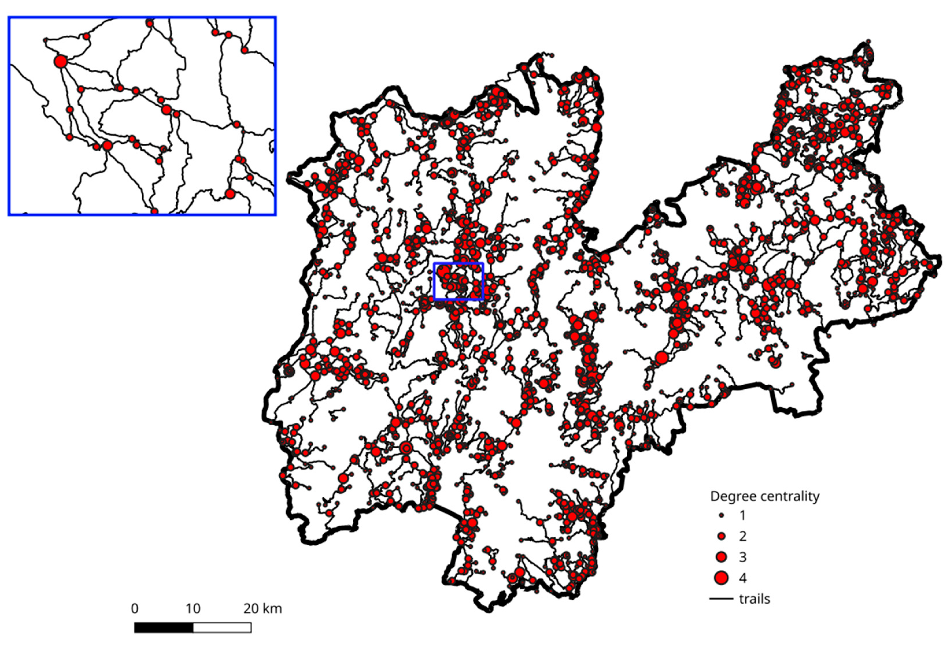
2.4. Local Connectivity Evaluation

In order to emphasize local topological aspects and look into potential discrepancies in various network segments, local metrics of connection have been assessed.

The number and positions of bridges and articulation points have been established by the first analysis. If and only if they are not a part of any cycle, arcs are bridges. Network connectivity is increased when a bridge is removed. Nodes that belong to each path between a certain pair of other nodes are known as articulation points, or cut points. The number of connected components rises as articulation points are eliminated.

Calculating the centrality measures of nodes in a network allows the determination of their relative importance [27]:

• degree centrality, which is the number of edges connecting a node;
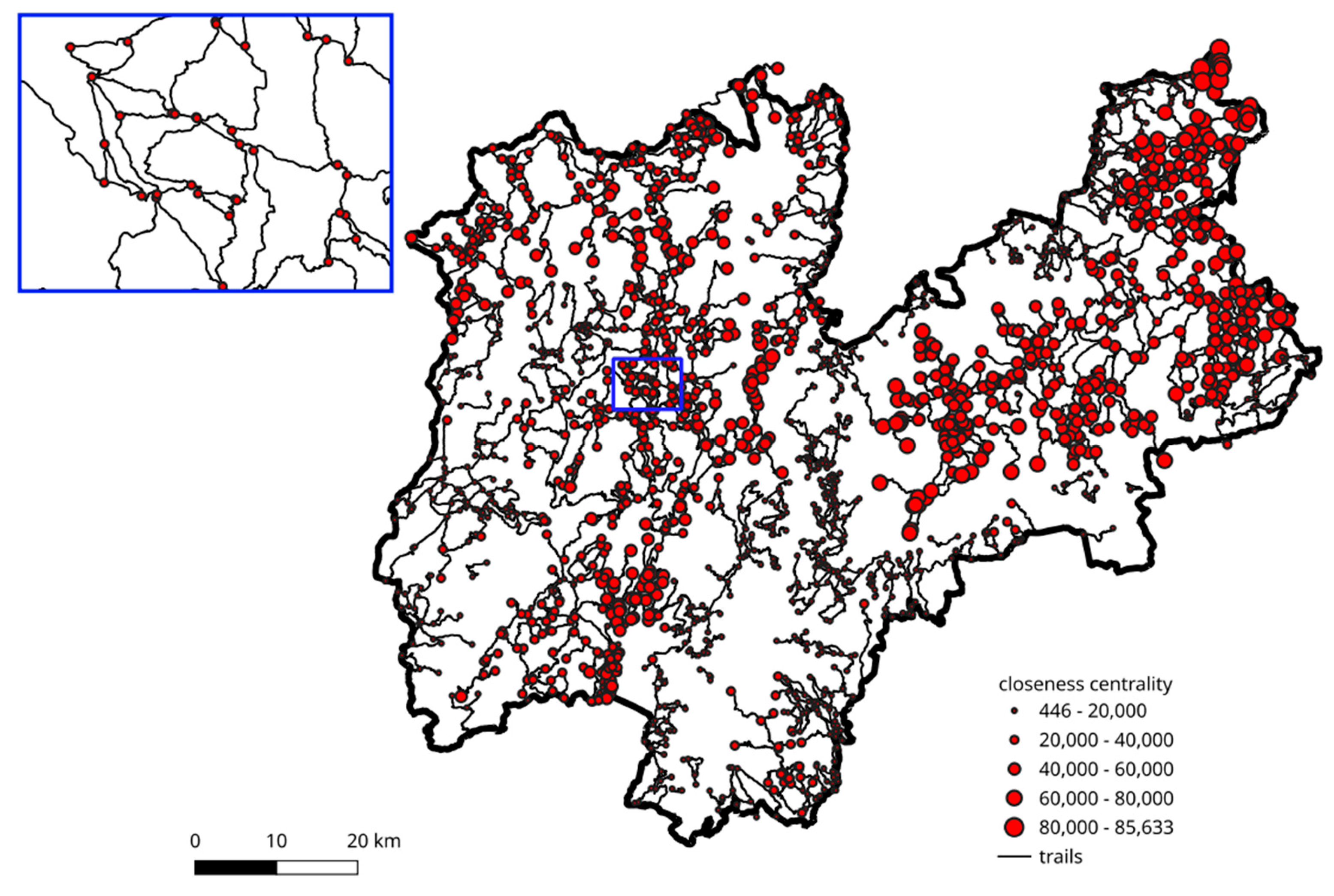
• closeness centrality, defined as the average length of the shortest path between a node and all the other nodes in the network; the more central a node is, the closer it is to all other nodes;
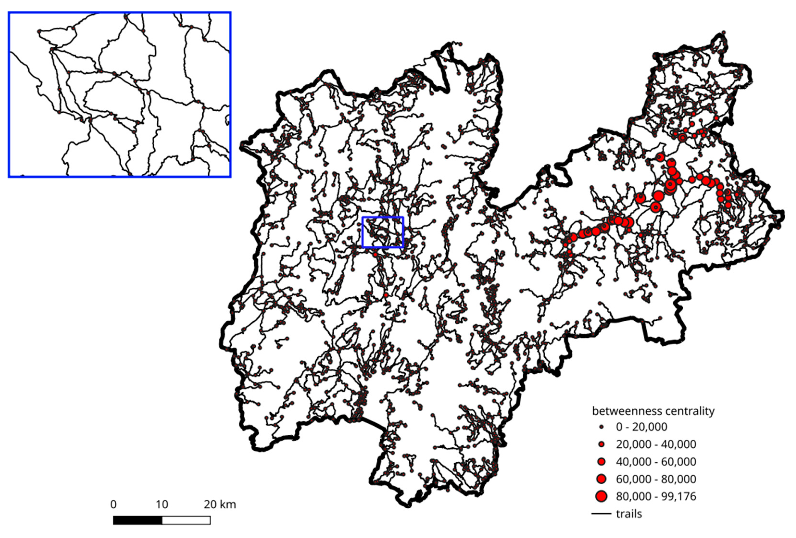
• betweenness centrality, measuring the average length of shortest paths between two any other nodes passing through the node; the value is 0 if no shortest path passes through the node;
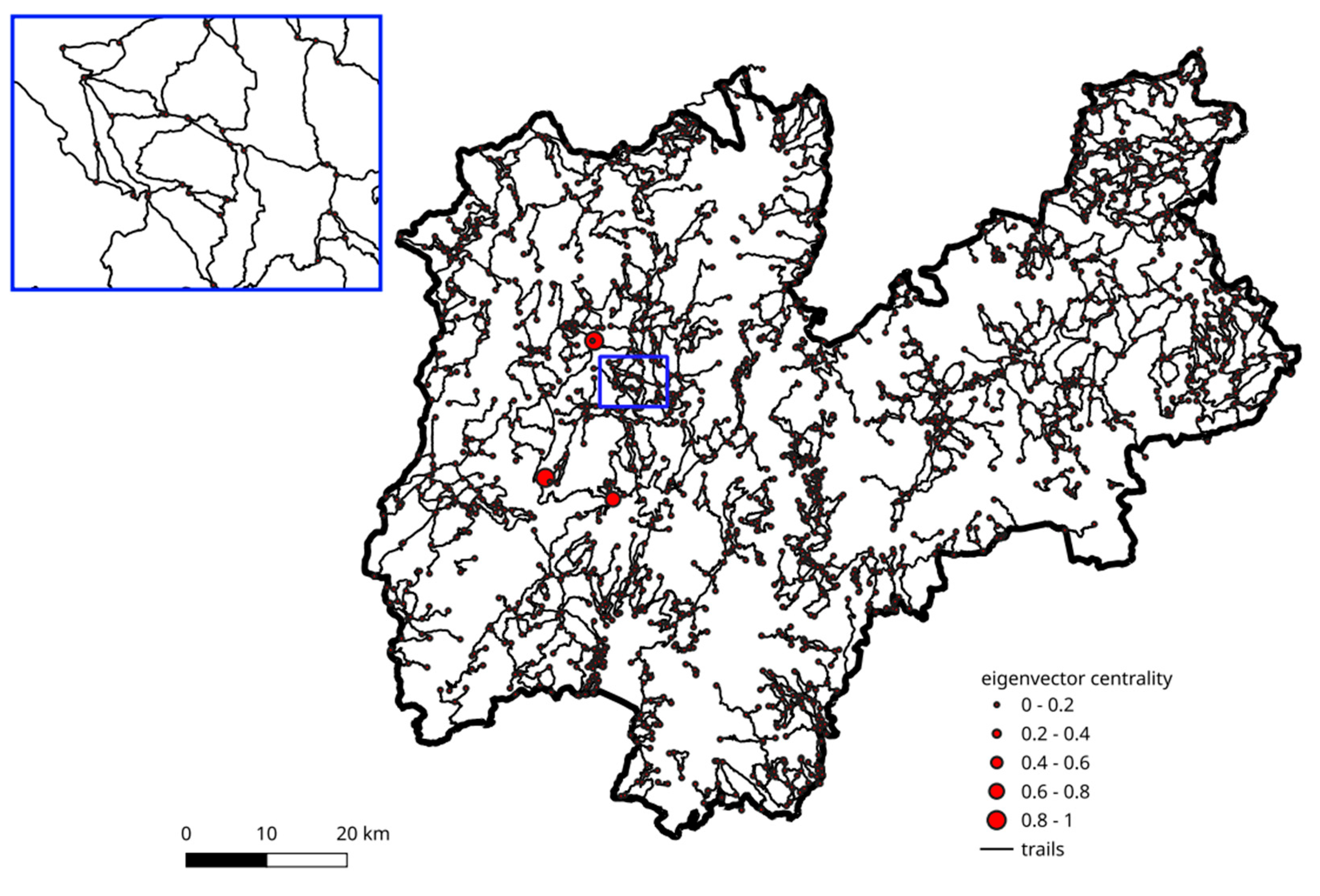
• eigenvector centrality, which assesses the influence of a node on a network by its connections to other nodes with high eigenvector centrality, i. e. a node is important if it is connected to important nodes; it is evaluated by a linear combination of the eigenvectors of the adjacency matrix.

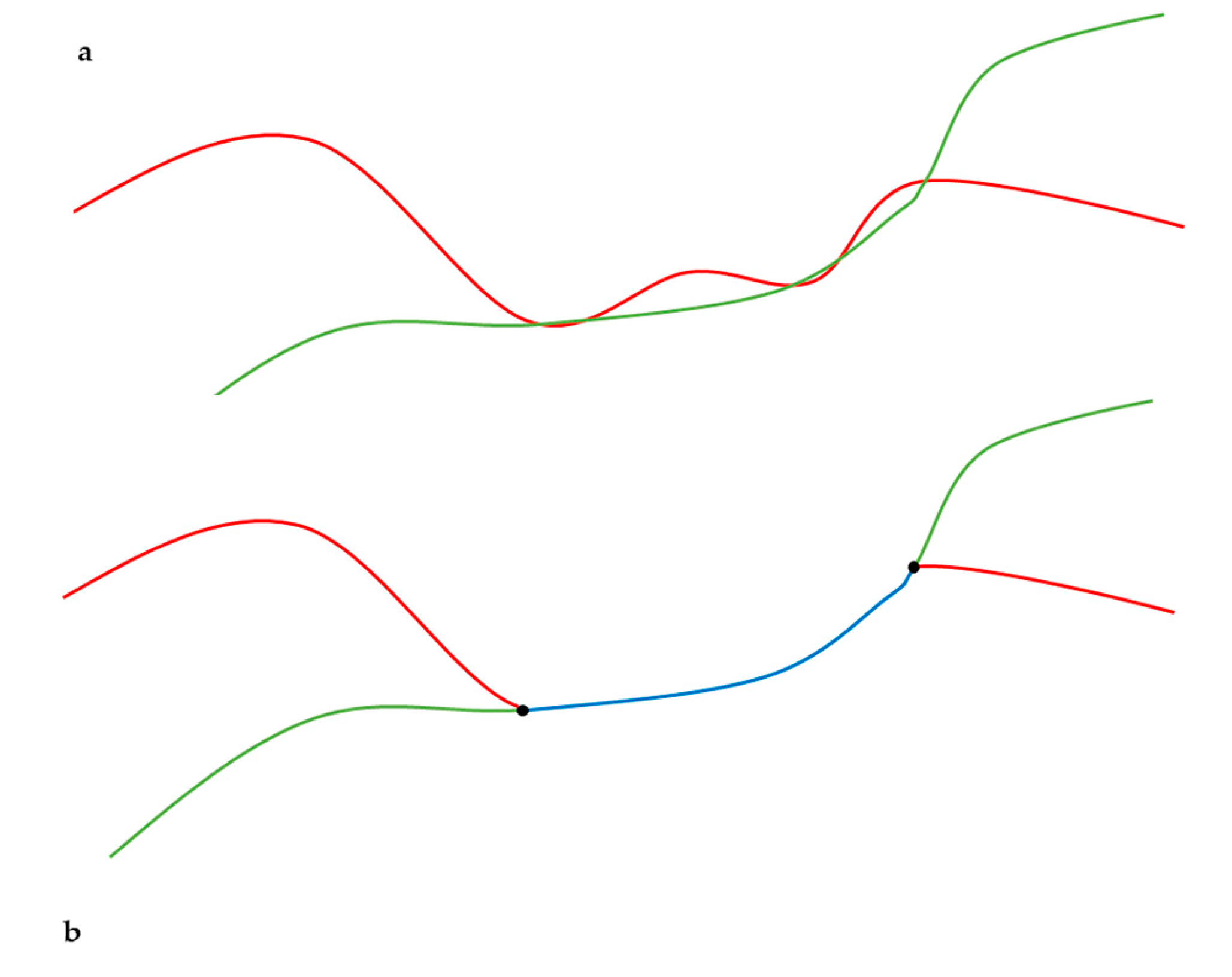
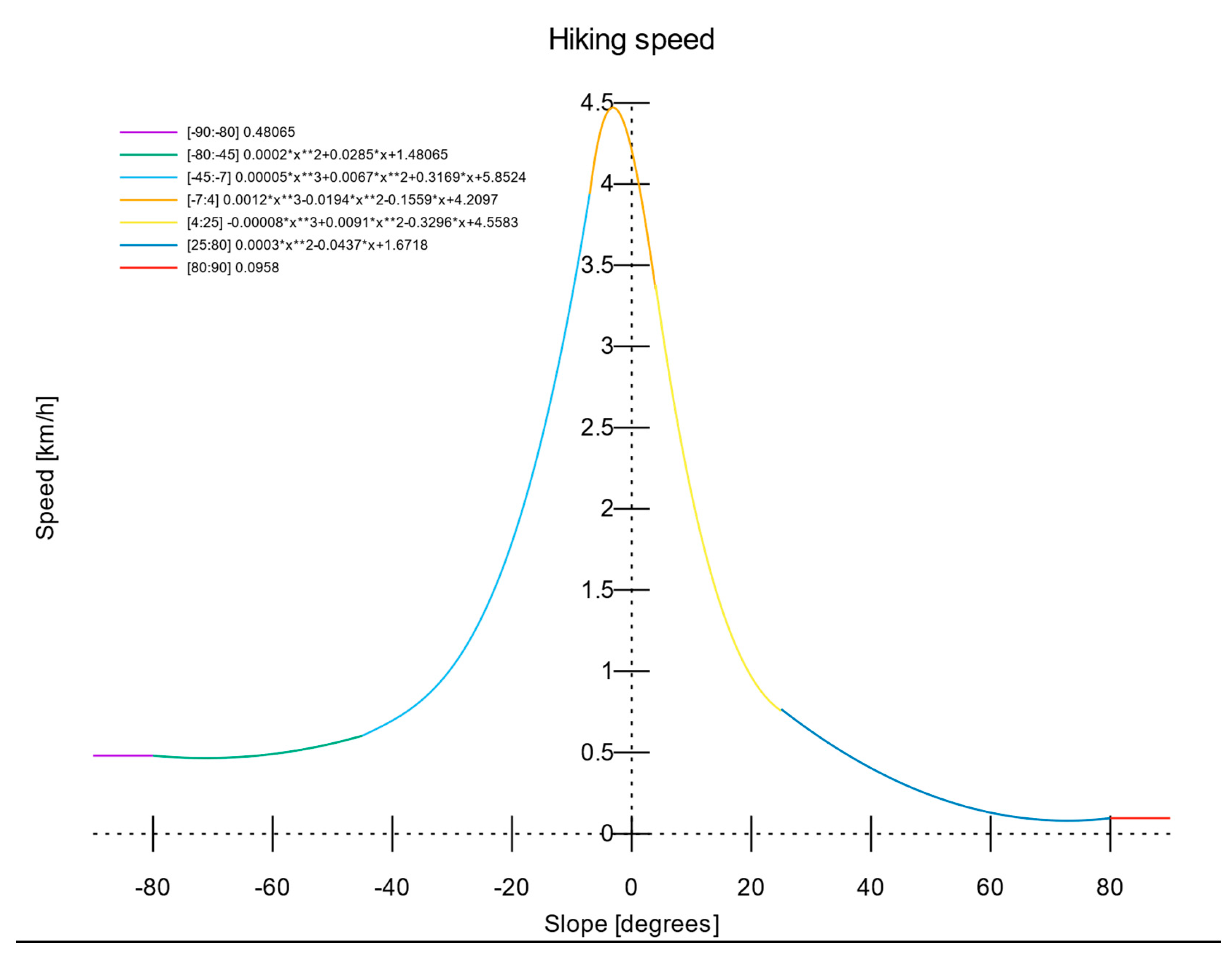
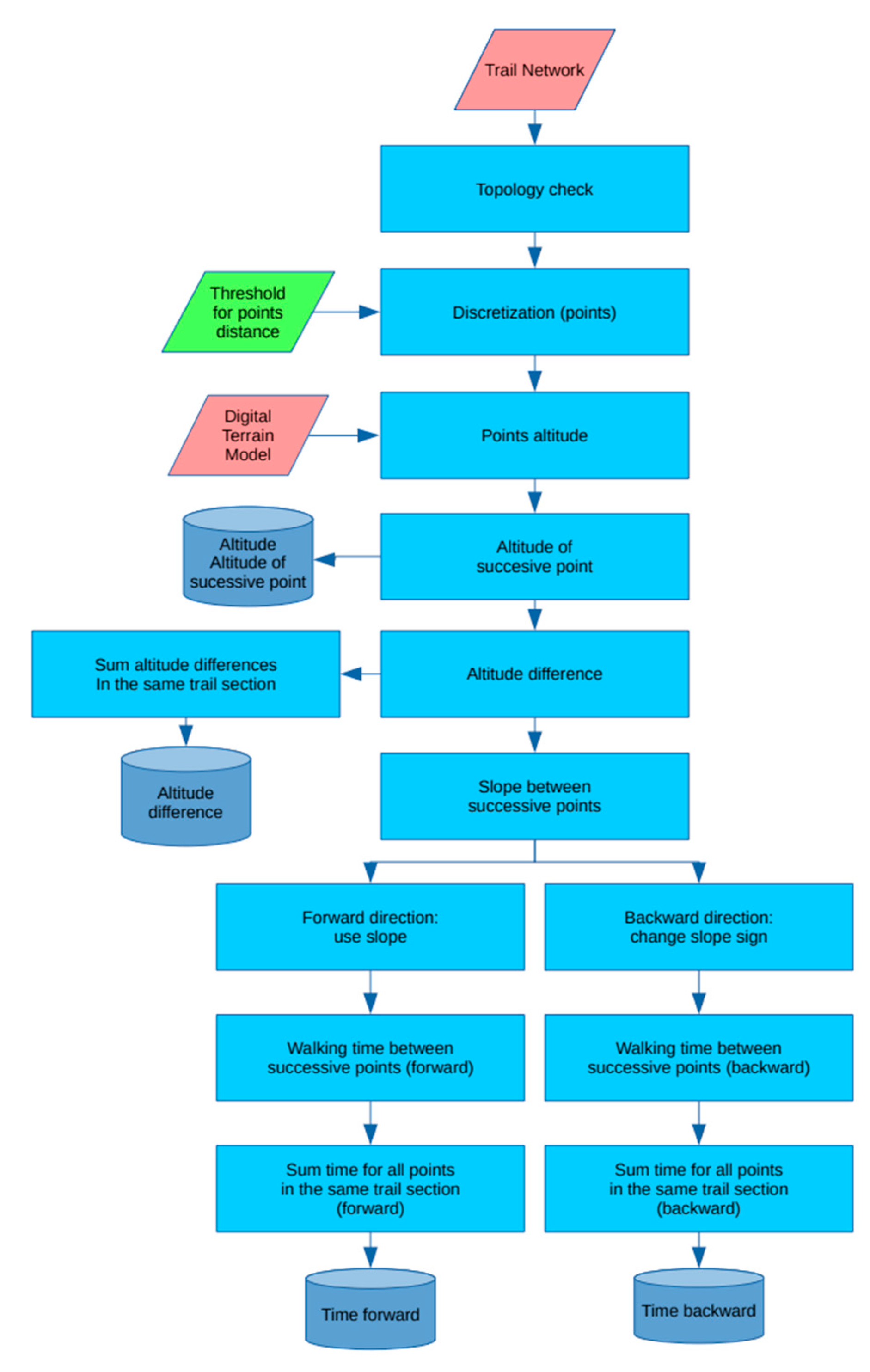
2.5. Route Optimization and Hiking Time Evaluation

Shorter routes between two places, shorter routes that travel through a specified group of points, and shorter ring routes that pass through a specified set of points are the three traditional network optimization problems that are resolved via route computation. This final scenario is known as the “Traveling Salesman Problem”, or “TSP,” and it involves the identification of the shortest route to get to every client and back to the base.

Operationally, the problem is solved by creating a graph with nodes that represent the traveling salesman’s headquarters and customer locations, and arcs that represent the paths connecting the nodes. The goal is to find a circular path that minimizes the distance between all of the nodes.

The problem, while simple to define, is somewhat complex to solve, since the number of its solutions grows very rapidly as the number of nodes increases [28].

The optimal route is determined by minimizing a “cost”, which usually corresponds to the geometric distance between two points. However, depending on the application, it may be wise to include additional characteristics as part of the “cost”; for example, mountain routes may have considerable altimetric fluctuations, making it more important to reduce the total altitude difference or trip time.

Hiking speed depends on may factors, both relating to the walking individual and the path’s features. The main parameter affecting walking speed is slope [29]. Its influence on walking speed has been investigated in controlled experiments on treadmills [30], on mock sloped walkway [31] and in urban environments [32].

Different formulations exist for hiking speed on natural paths [29,33], relating speed to horizontal distance, cumulative elevation gain and cumulative elevation loss, therefore to slope. In this application the travel times of the individual sections of the paths have been assessed in the two directions using the indications of the Swiss Body Pro Sentieri [34,35], which relate the walking speed of a standard person (adult individual in good physical condition but without specific athletic skills) with the slope of the path. This formulation has been chosen because it is simple and very fast. In fact, speed must be evaluated on a very large number of path sections into which each trail is discretized.

Therefore, a piecewise third degree polynomial is used to create a relationship between walking speed and path slope [36], as shown below in Table 2 and in Figure 4.

Additionally, it is feasible to implement penalizing coefficients based on the individual’s gender, age, and fitness level as well as the terrain’s features (height, terrain roughness, and vegetation density) [29,36,37]. In principle, it could be possible to take into account the time of the day to evaluate the walking time through a penalizing term. In fact, the time of the day influences the temperature and the visibility, which in turn influence the walking speed. However, since the time of the day would be the same for all the possible paths, this would not influence the choice of the optimal path.

While hiking time can be evaluated as a function of the slope with reasonable accuracy, this procedure is not available in any current GIS implementation. Therefore, this capability has been added to GRASS GIS with an original script which evaluates the travelling times and altitude differences for any arc and use them as costs in the shortest path evaluation. The script integrates the possibility to evaluate the walking time for an arbitrary segment of the network, making it possible to assign a time to each arc. It is then possible to apply a path optimization tool available in a GIS using this time as a cost.

3. Results

3.1. Global Connectivity Evaluation

The trail network comprises 2518 edges (e), 2016 nodes (n), and 66 isolated subgraphs (p) after nodes are created at intersections and duplicate lines are eliminated. Consequently, μ=478, α=0.12, β=1.20, and γ=0.40 for this network. With an average of 1.20 connections (edges) per node (β), these values show a medium level of connectivity. A medium level of connectivity is indicated by an intermediate value of γ, but a low value of α suggests a limited number of possible cycles. When combined, these numbers show a network structure between the grid arrangement and the core (tree).

The minimum spanning tree for the trail network (Figure 5), i.e., the sub network of minimum length connecting all the nodes, contains 2193 arcs out of the original 2681, for a total length of 3982.86 km instead of the original 5393.43 km. This means that only 81.80% of the arcs, corresponding to the 73.85% of the total trail network length, are needed to connect all the nodes.

3.2. Local Connectivity Evaluation

The Trentino trail network contains 899 bridges (Figure 6) and 793 articulation points (Figure 7). Trail sections constituting a bridge need particular maintenance since they are the only path to an ending node. At the same time, nodes representing articulation points must be careful maintained because they connect sub networks.

Table 3 shows the main features of the four centrality indexes, their spatial distribution is mapped in Figure 8, Figure 9, Figure 10 and Figure 11.

Figure 8 illustrates that, as anticipated, nodes in the sub network’s centers have higher degree centrality. Degree centrality ranges from 1 (a node connected by only one edge) to 5 (a node with five connections). More than half of the nodes may be reached by taking multiple trails, according to their median value of 3 of the centrality degree.

The average length of the shortest path between a node and every other node in the network, or closeness centrality, is 28209.08 m, with a wide range from 446.07 m to 85633.16 m. While nodes in the northeastern portion of the network correlate with higher levels of proximity, nodes with averagely short connections are found in the periphery of the subnetworks (Figure 9).

Betweenness centrality has a maximum value of 99176 m, corresponding to a node in the north east extremity of the network (Figure 10). The distribution of the values is very heterogeneous, with very high values in the east part of the network.

Finally, eigenvector centrality, which ranks the nodes depending on their connection to well-connected nodes, is maximum for two nodes in the eastern part of the network, with a third high ranking node nearby (Figure 11).

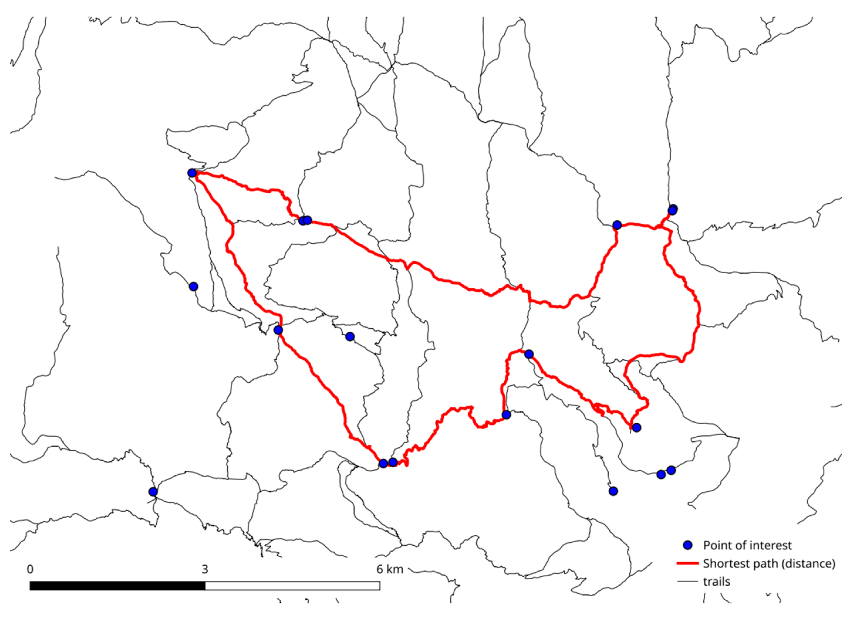
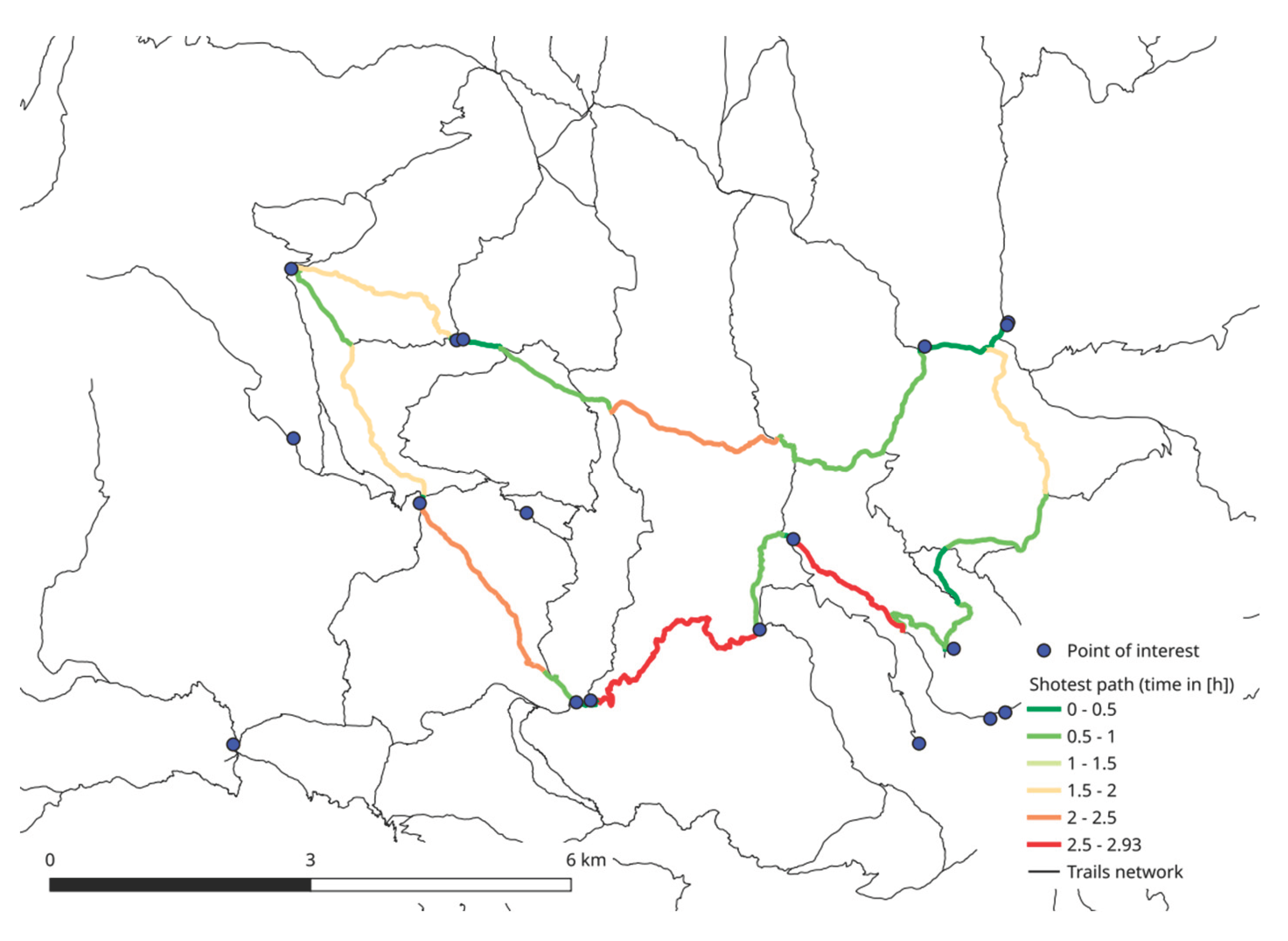
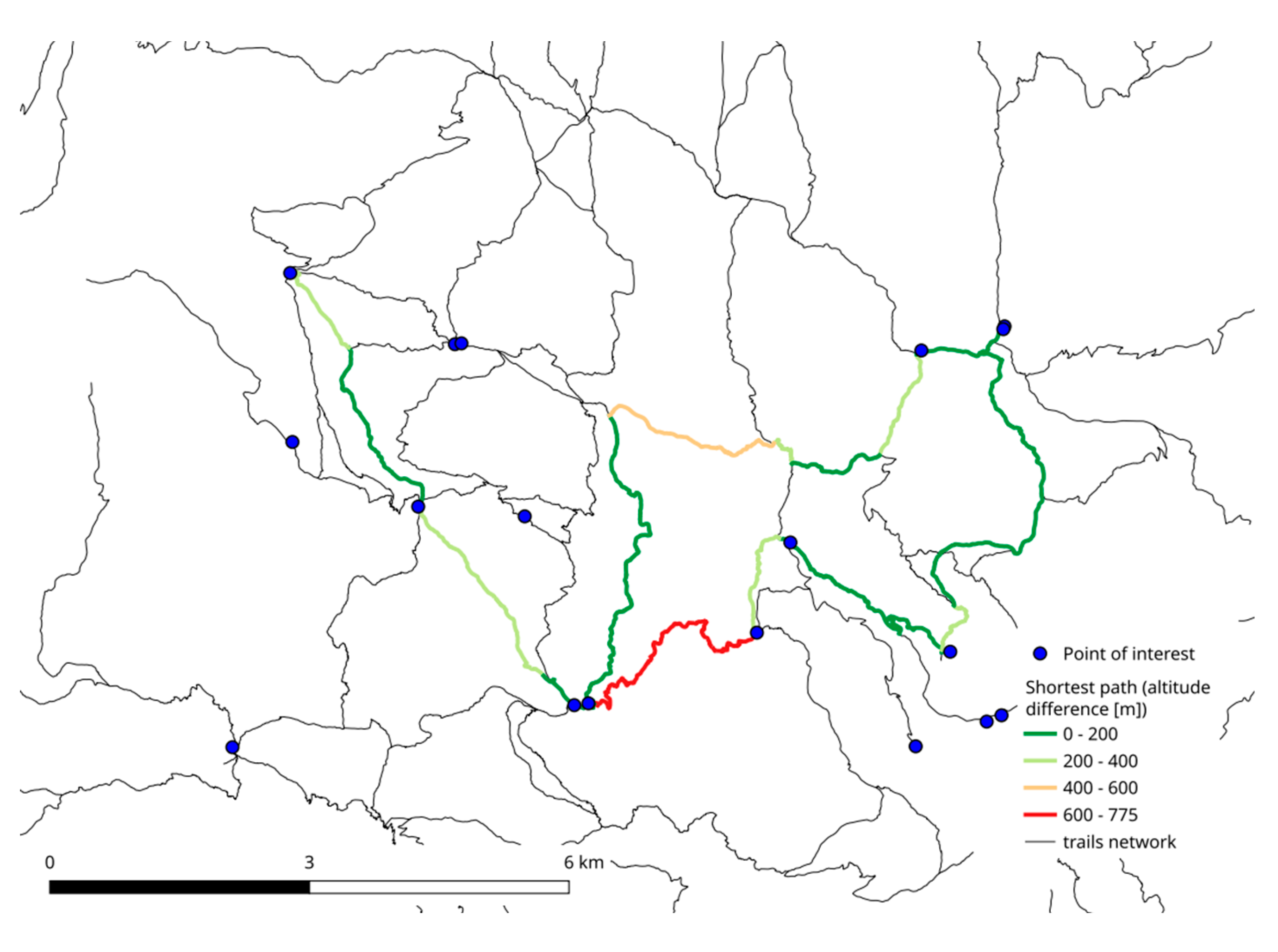
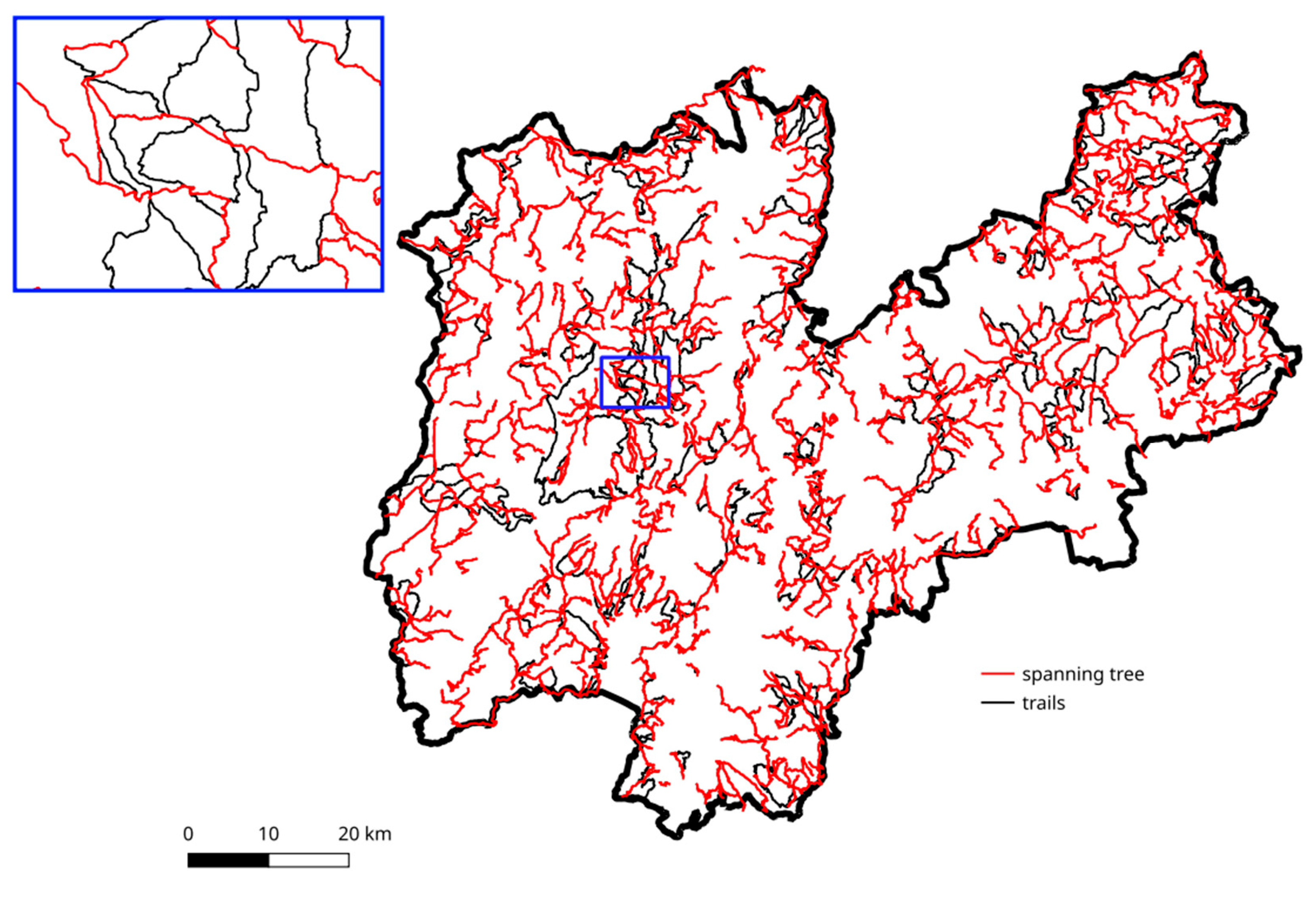
3.3. Paths Optimization

The route optimization methods have been applied to a sub set of the trail network, in the central west part of the region (Figure 2). This area corresponds to the Brenta mountain group (Figure 12) and includes 47 of the 1079 Trentino trails, for a length of 119,975 meters, compared to 5,598,680 meters of the entire trail network, i.e., 2.1% of the total. 15 refuges, 2 huts (“baita” or “baito”) and 2 high mountain pasture huts (“malga”) have been added to the network, to be used as points of interest for path optimization.

Table 4. Elevations and names of points of interest used as nodes for optimal paths determination.

Point of interest	Elev. [m]	Point of interest	Elev. [m]
Rifugio Croz dell’Altissimo	1,441	Baita Ciclamino	927
Rifugio Montanara	1,507	Baito Brenta Alta	1,668
Rifugio Pedrotti	2,500	Malga Cavedago	1,852
Rifugio Pradél	1,364	Malga Spora	1,857
Rifugio Sella	2,282	Rifugio Alberto e Maria ai Brentei	2,179
Rifugio Selvata	1,656	Rifugio Alimonta	2,589
Rifugio Tosa	2,449	Rifugio Brenta	1,357
Rifugio Tuckett	2,270	Rifugio Cacciatori di Spora	1,868
Rifugio XII Apostoli	2,490	Rifugio Casinei	1,825

Table 4. Elevations and names of points of interest used as nodes for optimal paths determination.

Point of interest	Elev. [m]	Point of interest	Elev. [m]
Rifugio Croz dell’Altissimo	1,441	Baita Ciclamino	927
Rifugio Montanara	1,507	Baito Brenta Alta	1,668
Rifugio Pedrotti	2,500	Malga Cavedago	1,852
Rifugio Pradél	1,364	Malga Spora	1,857
Rifugio Sella	2,282	Rifugio Alberto e Maria ai Brentei	2,179
Rifugio Selvata	1,656	Rifugio Alimonta	2,589
Rifugio Tosa	2,449	Rifugio Brenta	1,357
Rifugio Tuckett	2,270	Rifugio Cacciatori di Spora	1,868
Rifugio XII Apostoli	2,490	Rifugio Casinei	1,825

The network that was created in this way was utilized in GRASS GIS to identify the trails’ pathways that minimized the planimetric distance, travel duration, and uphill altitude difference for each segment of the path.

The entire process is automated and only requires a vector map with the trail network and a DTM to calculate slope and elevation changes and assess walking times. It has been implemented in a Python script in GRASS GIS 8.4 and is accessible on a GitHub repository [38].

The routes were divided into 10-meter segments, and altitude, slope, and travel speed were computed in both directions for each segment. This is because the slope of a stretch can cause its cost to vary greatly depending on which way it is traveled. The graph and the computation model that was used are therefore asymmetrical.

The altitude is obtained from a DTM with a resolution of 10 m [20]. The optimal DTM resolution depends on the sinuosity of the lines representing the trails and on the steepness of the area because the altitude is sampled on points at a constant distance interval: for flat areas DTM resolution is obviously irrelevant, for convolute trail the DTM must have a resolution high enough to detect the different altitudes of the sample points.

According to earlier tests on a few routes in the Vigolana mountain group in central Trentino [36], employing DTMs with better resolution results in a notable variation in the estimation of trip durations, but only for short and curving roads.

It is therefore possible to evaluate the elevation change in the traveling direction, which corresponds to the forward or backward direction for the arc, the slope and the time required for each arc in both directions (Table 5). These values are added for each arc in the database table of the map describing the trail network, using columns created for this purpose. This information is used by the routing algorithm to find the shortest path. The procedure for the time and altitude evaluation is shown in Figure 13.

The travel times calculated using this technique were contrasted with the SAT’s reported times, i.e., with the hiking times quoted by the organization managing the trails network in the Trentino region. An example is in Table 6. Good agreements were found, with an underestimation of the times in some cases, also taking into account the fact that published times have typically a 15’ resolution, while times are calculated with 1’ resolution.

The approach has been tested on a close loop itinerary starting from the Casinei refuge. It begins at an elevation of 1825 meters at Casinei refuge and travels through the Tosa refuge (2449 meters), the Montanara refuge (1506 meters), and Malga Cavedago (1852 meters). Three optimal routes were identified using the planimetric distance, travel time, and altitude difference as the cost to be minimized. The distance, travel duration, and altitude difference for the three best routes are displayed in Table 7.

A different choice of the quantity to be minimized determines optimal routes with significantly different characteristics, for example minimizing the difference in altitude increases the distance by about 20% compared to the shortest route and the walking time by about 27% compared to the fastest route. Figure 14 to Figure 16 show the three minimum routes: it is possible to note that some sections are selected whatever the cost (distance, time or difference in altitude) that is minimized, while other sections change, especially in the eastern part of the map.

Figure 14. Path minimizing planimetric distance.

Figure 14. Path minimizing planimetric distance.

Figure 15. Path minimizing travel time.

Figure 15. Path minimizing travel time.

Figure 16. Path minimizing slope (uphill altitude difference).

Figure 16. Path minimizing slope (uphill altitude difference).

4. Discussion

The availability of the digital map of Trentino mountain trails with CC0 1.0 Universal (CC0 1.0) Public Domain Dedication license creates the opportunity for a variety of intriguing analysis and applications for network administrators and users alike.

Any analysis of this kind must first check and correct the map’s topology, moving from a map that corresponds to a simple set of lines that represent the paths to a network configuration with nodes at every junction and no duplicate arcs.

The analysis of the trail network topology has indicated some interesting features, such as the heterogeneity of the centrality of the nodes, with few high rank nodes with respect to the eigenvalue centrality. The network structure lies between the grid configuration and the core (tree), which is similar to the configuration of the trail network of the Peneda-Gerês National Park (Portugal) reported by Kołodziejczyk [11].

Conversely, again Kołodziejczyk [11] indicates a grid configuration for the Krkonoše National Park (Czech Republic), while for a smaller recreational area in Austria Taczanowska et al. [12] indicate a core configuration.

Using the procedure implemented in this research, it is possible to assign variations in altitude and journey duration to each network arch by automatically calculating these quantities. This allows for the use of these quantities as costs to calculate optimal routes. The results of the test indicate that different optimization parameter choices result in notably different paths.

In terms of points of interest, distance, slope, and travel time, the current study offers hikers an effective tool to personalize the routes according to their tastes. The benefit of this kind of service is that it can help people get the most out of their outdoor leisure activities in mountainous regions. The demand and preferences of hikers and visitors for Cultural Ecosystem Services (CES) [39] are being studied more and more, and the supply of these services is being mapped both locally and worldwide [40,41]. In actuality, hikers’ attitudes and the natural setting in which they are experienced combine to produce outdoor recreational activities [42,43].

In order to fully capitalize on the allure of the mountain regions and to optimize tourism experiences, the analyses presented in this study can be utilized to effectively manage the trail networks [44], by adding specific POIs (focus points) or modifying the costs associated with arcs with a particular interest (for example scenic routes).

Additionally, it is well known that the provision of CES creates a stream of benefits with quantifiable and substantial economic value [inter alia 45–47], which should be considered when creating management plans.

The studies in the preceding sections may be a helpful tool for network managers to handle competing interests in use [48]. Interpersonal conflict has been the primary focus of the literature on this subject, i.e., when “another person’s behaviour can actually alter the desired social or physical components of the recreation experience” [48] (p.369). Examples of these conflicts are the ones rising between hunters and non-hunters [49], hikers and mountain bikers [50], alpine skiers and snowboarders [51].

Additionally, the inevitable trade-off between enjoyment and conservation in natural settings should be addressed via trail network management [52]. Recreational activities can improve consumers’ well-being and personal pleasure while also generating income for conservation initiatives [53]. Recreational activities, however, have the potential to negatively affect the ecosystem’s “natural” dynamics. Given this, the current study intends to serve as the foundation for developing a tool that can assist managers in setting priorities for both routine and exceptional investments as well as in creating conflict-reduction policies.

The approach is applicable to any trail network, as long as a DTM with a reasonable resolution and the trail network vector map are available. For trails at high altitude the function evaluating the speed from the slope value is probably less reliable, but for this type of analysis it is important the ratio between the time costs of different paths, not their absolute values.

The limitations of this approach lie in the evaluation of the hiking speed, therefore the time needed for each trail section, which depends only on the slope, neglecting other parameters which can influence the walking speed, such as terrain roughness, vegetation density, altitude and the physical features of the hikers. However, the influence of these parameters on the walking speed is difficult to evaluate even in the few locations where the relevant data are available.

The tools presented in this paper can also be used to support the design of new itineraries based on a network of existing paths. For example, naturalistic-cultural itineraries for new forms of sustainable and responsible tourism to support local development [18].

Following Taczanowska et al. [12], the study will continue, specifically with regard to connectivity, by examining the actual usage of the trail network through the analysis of GPS tracks that hikers have contributed to websites that gather information about routes and amateur sports performances.

In addition to the conventional points of interest, such as car parks, huts, and refuges, other points of interest could be included based on an inter-visibility analysis for the automatic calculation of the panorama spots.

Additionally, the use of different sets of arcs and nodes costs depending on the interests of different hikers groups, for example taking into account the scenery or the floristic interest, are being investigated.

The Python script for the walking time evaluation will be converted into a GRASS addon module and released under the GNU Public License.

Finally, it will be possible to publish the path optimization procedure as a webgis service. The determination of the optimal route can be done directly in a database management systems (DBMS), such as PostreSQL [54] using PostGIS’ [55] pgRouting library [56] in real time. PostreSQL is a powerful Open Source DBMS which can easily interfaced with a WebGIS [57], and its pgRouting extension adds network analysis capabilities [58]. The determination of the walking time for each network arc is time consuming, but it can be executed beforehand, storing the results in the table associated to the vector map representing the trail network.

5. Conclusions

The digital SAT map with CC0 1.0 Universal (CC0 1.0) Public Domain Dedication license offers numerous analyses for network managers and users.

Automatic determination of height and travel times allows for cost minimization in route calculation. Different optimization parameters lead to significantly different paths, highlighting the potential for improved network management. In terms of points of interest, distance, slope, and journey duration, the current study offers hikers an effective tool to personalize the routes according to their preferences. Network managers can use these analyses to manage conflicts between interests in use, such as hunting and non-hunting, hiking and mountain biking, and alpine skiers and snowboarders. The management of trails network must balance conservation and recreation, as recreational activities can generate revenue for conservation interventions and benefit users but can also interfere with ecosystem dynamics.

References

1. Hagget, P.; Chorley, R.J. Network analysis in geography, London: Arnold, England, 1974. 1974. [Google Scholar]
2. Arlinghaus, S.L.; Arlinghaus, W.C.; Harary, F. Graph Theory and Geography: An Interactive View; John Wiley and Sons: New York, USA, 2002. [Google Scholar]
3. Ghosh, S.; Mallick, A.; Chowdhury, A.; De Sarkar, K.; Mukherjee, J. Graph theory applications for advanced geospatial modelling and decision-making. Appl. Geomat. 2024, 16, 799–812. [Google Scholar] [CrossRef]
4. Phillips, J.D.; Schwanghart, W.; Heckmann, T. Graph theory in the geosciences. Earth-Sci. Rev. 2015, 143, 147–160. [Google Scholar] [CrossRef]
5. Gobbi, S.; Cantiani, M. G.; Rocchini, D.; Zatelli, P.; Tattoni, C.; La Porta, N.; Ciolli, M. Fine spatial scale modelling of Trentino past forest landscape (Trentinoland): A case study of FOSS application. Int. Arch. Photogramm. Remote Sens. Spat. Inf. Sci. - ISPRS Arch. 2019, 42, 71–78. [Google Scholar] [CrossRef]
6. Zatelli, P.; Gobbi, S.; Tattoni, C.; La Porta, N.; Ciolli, M. (20. Object-based image analysis for historic maps classification. Int. Arch. Photogramm. Remote Sens. Spat. Inf. Sci. - ISPRS Arch. 2019, 42, 247–254. [Google Scholar] [CrossRef]
7. Gobbi, S.; Ciolli, M.; La Porta, N.; Rocchini, D.; Tattoni, C.; Zatelli, P. New Tools for the Classification and Filtering of Historical Maps. ISPRS Int. J. Geo-Inf. 2019, 8, 455. [Google Scholar] [CrossRef]
8. Ferretti, F.; Sboarina, C.; Tattoni, C.; Vitti, A.; Zatelli, P.; Geri, F.; Pompei, E.; Ciolli, M. The 1936 Italian Kingdom Forest Map reviewed: A dataset for landscape and ecological research. Ann. Silvic. Res. 2018, 42, 3–19. [Google Scholar] [CrossRef]
9. Gobbi, S.; Maimeri, G.; Tattoni, C.; Cantiani, M. G.; Rocchini, D.; La Porta, N.; Ciolli, M.; Zatelli, P. Orthorectification of a large dataset of historical aerial images: Procedure and precision assessment in an open source environment. Int. Arch. Photogramm. Remote Sens. Spat. Inf. Sci. - ISPRS Arch. 2018, 42, 53–59. [Google Scholar] [CrossRef]
10. PAT, Tracciati alpini. Available online: https://siat.provincia.tn.it/geonetwork/srv/ita/catalog.search#/metadata/p_TN:f3547bc8-bf1e-4731-85d2-2084d1f4ba07 (accessed on 2 March 2025).
11. Kołodziejczyk, K. Networks of hiking tourist trails in the Krkonoše (Czech Republic) and Peneda-Gerês(Portugal) national parks – comparative analysis. J. Mt. Sci. 2019, 16, 725–743. [Google Scholar] [CrossRef]
12. Taczanowska, K.; González, L.M.; Garcia-Massó, X.; Muhar, A.; Brandenburg, C.; Toca-Herrera, J.L. (2014) Evaluating the structure and use of hiking trails in recreational areas using a mixed GPS tracking and graph theory approach. Appl. Geogr. 2014, 55, 184–192. [Google Scholar] [CrossRef]
13. PAT, Rifugi e bivacchi. Geocatalogo della Provincia Autonoma di Trento. Available online: https://siat.provincia.tn.it/geonetwork/srv/eng/catalog.search#/metadata/p_TN:f3547bc8-bf1e-4731-85d2-2084d1f4ba07 (accessed on 2 March 2025).
14. Kolkos, G.; Kantartzis, A.; Stergiadou, A.; Arabatzis, G. Development of Semi-Mountainous and Mountainous Areas: Design of Trail Paths, Optimal Spatial Distribution of Trail Facilities, and Trail Ranking via MCDM-VIKOR Method. Sustainability 2024, 16, 9966. [Google Scholar] [CrossRef]
15. Tomczyk, A. M.; Ewertowski, M. Planning of recreational trails in protected areas: Application of regression tree analysis and geographic information systems, Appl. Geogr., 2013, 40, 129–139. [Google Scholar] [CrossRef]
16. Snyder, S. A.; Whitmore, J. H.; Schneider, I. E.; Becker, D. R. Ecological criteria, participant preferences and location models: A GIS approach toward ATV trail planning, Appl. Geogr., 2008, 28, 248–258. [Google Scholar] [CrossRef]
17. Chiou, C.; Tsai, W.; Leung, Y. A GIS-dynamic segmentation approach to planning travel routes on forest trail networks in Central Taiwan, Landsc. Urban Plan., 2010, 97 (4), 221-228. [CrossRef]
18. Zatelli, P.; Gabellieri, N.; Besana, A. In the footsteps of grandtourists: Envisioning itineraries in inner areas for literary and responsible tourism. ISPRS Int. J. Geo-Inf. 2025, 14, 67. [Google Scholar] [CrossRef]
19. Società Alpinisti Tridentini (SAT), Rete sentieri Trentino – Catasto. Available online: https://www.sat.tn.it/sentieri/catasto/ (accessed on 2 March 2025).
20. PAT, Modello digitale del terreno per idrologia, Geocatalogo della Provincia Autonoma di Trento. Available online: https://siat.provincia.tn.it/geonetwork/srv/ita/catalog.search#/metadata/p_TN:d6472d5e-94b7-456e-b633-0bf19daf6cdf (accessed on 2 March 2025).
21. GRASS Development Team, 2024. Geographic Resources Analysis Support System (GRASS) Software, Version 8.4. Open Source Geospatial Foundation. Available online: https://grass.osgeo.org (accessed on 2 March 2025).
22. Neteler, M.; Bowman, M.; Landa, M.; Metz, M. GRASS GIS: A multi-purpose Open Source GIS. Environ. Model. Softw. 2012, 31, 124–130. [Google Scholar] [CrossRef]
23. Ciolli, M.; Federici, B.; Ferrando, I.; Marzocchi, R.; Sguerso, D.; Tattoni, C.; Vitti, A.; Zatelli, P. FOSS tools and applications for education in geospatial sciences. ISPRS Int. J. Geo-Inf. 2017, 6, 225. [Google Scholar] [CrossRef]
24. GRASS Development Team, 2025. Directed Graph Library. Available online: https://grass.osgeo.org/programming8/dglib.html (accessed on 30 May 2025).
25. Gattuso, D.; Miriello, E. Compared Analysis of Metro Networks Supported by Graph Theory. Netw Spat Econ 2005, 5, 395–414. [Google Scholar] [CrossRef]
26. Unwin, D. J. Introductory Spatial Analysis, Methuen &Co. Ltd.: London, England, 1981.
27. Borgatti, S.; Everett, M. A Graph-Theoretic Perspective on Centrality. Soc. Netw. 2006, 28, 466–484. [Google Scholar] [CrossRef]
28. Reinelt, G. The traveling salesman: Computational solutions for TSP applications, Springer-Verlag: Berlin Heidelberg, Germany, 1994.
29. Prisner, E.; Sui, P. Hiking-time formulas: a review. Cartogr. Geogr. Inf. Sci. (CaGIS) 2023, 50, 421–432. [Google Scholar] [CrossRef]
30. Kafetzakis, I.; Konstantinou, I.; Mandalidis, D. Effects of Hiking-Dependent Walking Speeds and Slopes on Spatiotemporal Gait Parameters and Ground Reaction Forces: A Treadmill-Based Analysis in Healthy Young Adults. Appl. Sci. 2024, 14, 4383. [Google Scholar] [CrossRef]
31. Xie, W.; Wai Ming Lee, E.; Li, T.; Jiang, N.; Ma, Y. Pedestrian dynamics on slopes: Empirical analysis of level, uphill, and downhill walking. Saf. Sc. 2024, 172, art. no. 106429. [Google Scholar] [CrossRef]
32. Nong, T.; Zhang, Z.; Wang, T.; Zhang, W.; Tan, J.; Lee, E.W.M.; Shi, M. Dynamics analysis of pedestrian movement on slopes: Modelling, simulations and experiments. Physica A. Stat. Mech. Appl. 2025, 668, 130589. [Google Scholar] [CrossRef]
33. Wood, A.; Mackaness, W.; Simpson, T.I.; Armstrong, J.D. Improved prediction of hiking speeds using a data driven approach. PLoS ONE 2023, 18, e0295848. [Google Scholar] [CrossRef]
34. Club Alpino Svizzero (AS). La formula delle escursioni Un risultato altamente scientifico, 2013. Available online: https://www.sac-cas.ch/it/le-alpi/la-formula-delle-escursioni-25135/ (accessed on 2 March 2025).
35. Club Alpino Italiano (CAI). Luoghi 2.0. Manuale on-line. Documenti. Tempi di percorrenza. Available online: https://luoghi.cai.it/manuale/index.htm (accessed on 2 March 2025).
36. Ciolli, M.; Mengon, L.; Vitti, A.; Zatelli, P.; Zottele, F. A GIS-based decision support system for the management of SAR operations in mountain areas. Geomatics Workbooks 2006, 6, 1–17. [Google Scholar]
37. Pitman, A.; Zanker, M.; Gamper, J.; Andritsos, P. Individualized Hiking Time Estimation. In 23rd International Workshop on Database and Expert Systems Applications, 2012, 101–105. [CrossRef]
38. Zatelli, P. 2025. Code repository to evaluate hiking times in GRASS GIS. Available online: https://github.com/pzatelli/hikingtimes (accessed on 30 May 2025).
39. Palacio Buendía, A.V.; Pérez-Albert, Y.; Serrano Giné, D. Mapping Landscape Perception: An Assessment with Public Participation Geographic Information Systems and Spatial Analysis Techniques. Land 2021, 10, 632. [Google Scholar] [CrossRef]
40. Vrbičanová, G.; Kaisová, D.; Močko, M.; Petrovič, F.; Mederly, P. Mapping Cultural Ecosystem Services Enables Better Informed Nature Protection and Landscape Management. Sustainability 2020, 12, 2138. [Google Scholar] [CrossRef]
41. Zoderer, B. M.; Tasser, E.; Erb, K. H.; Stanghellini, P. S. L.; Tappeiner, U. Identifying and mapping the tourists perception of cultural ecosystem services: A case study from an Alpine region. Land use policy 2016, 56, 251–261. [Google Scholar] [CrossRef]
42. Márquez-Pérez, J.; Vallejo-Villalta, I.; Álvarez-Francoso, J.I. Estimated travel time for walking trails in natural areas, Geografisk Tidsskrift-Danish Journal of Geography 2017, 117:1, 53-62. 117:1. [CrossRef]
43. Pettebone, D.; D’Antonio, A.; Sisneros-Kidd, A.; Monz, C. Modeling visitor use on high elevation mountain trails: An example from Longs Peak in Rocky Mountain National Park, USA. J. Mt. Sci. 2019, 16, 2882–2893. [Google Scholar] [CrossRef]
44. Bachi, L.; Carvalho Ribeiro, S.; Hermes, J.; Saadi, A. Cultural Ecosystem Services (CES) in landscapes with a tourist vocation: Mapping and modeling the physical landscape components that bring benefits to people in a mountain tourist destination in southeastern Brazil. Tour. Manag. 2020, 77, 104017. [Google Scholar] [CrossRef]
45. De Groot, R.S.; Wilson, M.A.; Boumans, R.M.J. A typology for the classification, description and valuation of ecosystem functions, goods and services. Ecol. Econ. 2002, 41, 393–408. [Google Scholar] [CrossRef]
46. Brander, L. M.; De Groot, R.; Schägner, J. P.; Guisado-Goñi, V.; Van’t Hoff, V.; Solomonides, S.; McVittie, A.; Eppink, F.; Sposato, M.; Do, L.; Ghermandi, A.; Sinclair, M.; Thomas, R. Economic values for ecosystem services: A global synthesis and way forward. Ecosystem Services 2024, 66, 101606. [Google Scholar] [CrossRef]
47. Teoh, S. H. S.; Symes, W. S.; Sun, H.; Pienkowski, T.; Carrasco, L. R. A global meta-analysis of the economic values of provisioning and cultural ecosystem services. Sci. Total Environ. 2019, 649, 1293–1298. [Google Scholar] [CrossRef] [PubMed]
48. Jacob, G.R.; Schreyer, R. Conflict in Outdoor Recreation: A Theoretical Perspective. J. Leis. Res. 2018, 12, 368–380. [Google Scholar] [CrossRef]
49. Schroeder, S. A.; Fulton, D. C.; Cornicelli, L.; McInenly, L. E. Recreation conflict, coping, and satisfaction: Minnesota grouse hunters’ conflicts and coping response related to all-terrain vehicle users, hikers, and other hunters. J. Outdoor Recreat. Tour. 2020, 30, 100282. [Google Scholar] [CrossRef]
50. Bachinger, M.; Hafner, M.; Harprecht, P. Cultural and space-based factors influencing recreational conflicts in forests. The example of cyclists and other forest visitors in Freiburg (Germany). Eur. J. Cult. Manag. Policy 2024, 13, 12494. [Google Scholar] [CrossRef]
51. Happ, E.; Schnitzer, M. Ski touring on groomed slopes: Analyzing opportunities, threats and areas of con-flict associated with an emerging outdoor activity. J. Outdoor Recreat. Tour. 2022, 39, 100521. [Google Scholar] [CrossRef]
52. Marion, J. L. Trail sustainability: A state-of-knowledge review of trail impacts, influential factors, sustainability ratings, and planning and management guidance. J. Environ. Manag. 2023, 340, 117868. [Google Scholar] [CrossRef]
53. Sandifer, P.A.; Sutton-Grier, A.E.; Ward, B.P. Exploring connections among nature, biodiversity, ecosystem services, and human health and well-being: opportunities to enhance health and biodiversity conservation. Ecosyst. Serv. 2015, 12, 1–15. [Google Scholar] [CrossRef]
54. PostreSQL Project Steering Committee, 2025. PPostgreSQL: The World’s Most Advanced Open Source Relational Database. Available online: https://www.postgresql.org/ (accessed on 5 October 2025).
55. PostGIS Project Steering Committee, 2025. PostGIS, spatial and geographic objects for postgreSQL. Available online: https://postgis.net/ (accessed on 5 October 2025).
56. pgRouting Project Steering Committee, 2025. pgRouting, routing and other network analysis functionality for postgreSQL and PostGIS. Available online: https://pgrouting.org/ (accessed on 5 October 2025).
57. Simeoni, L.; Zatelli, P; Floretta, C. Field measurements in river embankments: validation and management with spatial database and webGIS. Natural Hazards, 2014, 71, 1453–1473. [Google Scholar] [CrossRef]
58. Zhang, L. , He, X. Route Search Base on pgRouting. In Software Engineering and Knowledge Engineering: Theory and Practice. Advances in Intelligent and Soft Computing; Wu, Y., Eds.; Springer: Berlin, Heidelberg, 2012, 115, 1003–1007. [Google Scholar] [CrossRef]
Figure 1. Location of the study areas for the trail network analysis (black contour) and path optimization (red circle).
Preprints 184054 g001
Figure 2. Trail network and tourist districts (Società degli Alpinisti Tridentini - Society of the Tridentine Mountaineers, SAT). The highlighted Brenta Dolomites area has been selected for the path optimization analysis.
Preprints 184054 g002
Figure 3. Example of topological correction when two trails are originally represented by two lines intersecting multiple times (a): the overlapping section is represented by a single line and two nodes are placed at the intersections (b).
Preprints 184054 g003
Figure 4. Piecewise polynomial function expressing speed with respect to slope.
Preprints 184054 g004
Figure 5. Minimum spanning tree for the trail network.
Preprints 184054 g005
Figure 6. Bridges (trail sections not part of any cycle) of the trail network.
Preprints 184054 g006
Figure 7. Articulation points (nodes belonging to every path between some pair of other nodes) of the trail network.
Preprints 184054 g007
Figure 8. Degree centrality (number of edges connecting a node) of the trail network nodes.
Preprints 184054 g008
Figure 9. Closeness centrality (average length of the shortest path between a node and all the other nodes in the network) of the trail network nodes.
Preprints 184054 g009
Figure 10. Betweenness centrality (average length of shortest paths between two any other nodes passing through the node) of the trail network nodes.
Preprints 184054 g010
Figure 11. Eigenvector centrality (influence of a node on the network) of the trail network nodes.
Preprints 184054 g011
Figure 12. Trail sub network used for the path optimization tests.
Preprints 184054 g012
Figure 13. Workflow chart of the time and altitude difference costs evaluation. Output values are stored in the database table associated to the trail network and are used as costs in the route optimization procedure.
Preprints 184054 g013