Submitted:
03 November 2025
Posted:
07 November 2025
You are already at the latest version
Abstract
We start with the ideas in the papers “Chakraborti et al., Properties and performance of the c-chart for attributes data, Journal of Applied Statistics, January 2008” and “Bayesian Control Chart for Number of Defects in Production Quality Control. Mathematics 2024, 12, 1903. https:// doi.org/10.3390/math12121903”; then we use the Jarrett (1979) data from “A Note on the Intervals Between Coal-Mining Disasters” and the analysis by Kumar et al., and by Zhang et al. From the analysis of all the papers data we get different results: the cause is that they use the Probability Limits of the PI (Probability Interval) as they were the Control Limits (so they name them) of the Control Charts (CCs): those authors do not extract the complete information from the statistical data of CCs from the data not normally distributed. The Control Limits in the Shewhart CCs are based on the Normal Distribution (Central Limit Theorem, CLT) and are not valid for non-normal distributed data: consequently, the decisions about the “In Control” (IC) and “Out Of Control” (OOC) states of the process are wrong. The Control Limits of the CCs are wrongly computed, due to unsound knowledge of the fundamental concept of Confidence Interval. Minitab and other software (e.g. JMP, SAS) use the “T Charts”, claimed to be a good method for dealing with “rare events”, but their computed Control Limits of the CCs are wrong. We will show that the Reliability Integral Theory (RIT) is able to solve these problems.
Keywords:
control charts
; poisson distribution
; exponential distribution
; TBE
; T Charts
; Minitab
; JMP
; Reliability Integral Theory
1. Introduction
Since 1989, the author (FG) tried to inform the Scientific Community about the flaws in the use of (“wrong”) quality methods for making Quality [1] and in 1999 about the GIQA (Golden Integral Quality Approach) showing how to manage Quality during all the activities of the Product and Process Development in a Company [2], including the Process Management and Control Charts (CC) for Process Control.
First we show how to deal correctly with c-Control Charts by analysing a literature case [3], which uses data of “Nonconformities in Printed CircuitBoards (example 7.3)” in the Montgomery book “Introduction to Statistical Quality Control 8th ed.” and the ideas in “Bayesian Control Chart for Number of Defects in Production Quality Control”, published in Mathematics 2024: it is quite interesting that in a “rejected paper” a Peer Reviewr wrote “The content of the paper is mainly centered on applied statistics and industrial statistics. Hence, in my opinion the journal Mathematics is not the best venue for this manuscript.” Decision 13 February 2025.
Later, we show how to deal correctly with I-CC (Individual Control Charts) by analysing a literature case comprising the famous data-set on coal-mining disasters of Jarrett (1979); these data are considered and analysed in [4,5].
We found very interesting the statements in the Excerpt 1:
We agree with the authors in the Excerpt 1, but, nevertheless, they did not realise the problem that we are giving here: wrong Control Limits in CCs for Rare Events, with data exponentially or Weibull distributed. See References…
Using the data in [3,4,5] with good statistical methods [6,7,8,9,10,11,12,13,14,15,16,17,18,19,20,21,22,23,24,25,26,27,28,29,30,31,32,33] we give our “reflections on Control Charts (CCs)”.
We will try to state that several papers (that are not cited here, but you can find in the “Garden of flowers” [24] and some in the Appendix C) compute in an a-scientific way (see the formulae in the Appendix C) the Control Limits of CCs for “Individual Measures or Exponential, Weibull and Gamma distributed data”, indicated as I-CC (Individual Control Charts); we dare to show, to the Scientific Community, how to compute the True Control Limits. If the author is right, then all the decisions, taken up today, have been very costly to the Companies using those Control Limits; therefore, “Corrective Actions” are needed, according to the Quality Principles, because NO “Preventive Actions” were taken [1,2,27,28,29,30,31,32,33,34,35,36]: this is shown through the suggested published papers. Humbly, given our strong commitment to Quality [34,35,36,37,38,39,40,41,42,43,44,45,46], we would dare to provide the “truth”: Truth makes you free [hen (“hic et nunc”=here and now)].
On 22nd of February 2024, we found the paper “Publishing an applied statistics paper: Guidance and advice from editors” published in Quality and Reliability Engineering International (QREI-2024, 1-17) [by C. M. Anderson-Cook, Lu, R. B. Gramacy, L. A. Jones-Farmer, D. C. Montgomery, W. H. Woodall; the authors have important qualifications and Awards]; since I-CC is a part of “applied statistics” we think that their hints will help: the authors’ sentence “Like all decisions made in the face of uncertainty, Type I (good papers rejected) and Type II (flawed papers accepted) errors happen since the peer review process is not infallible.” is very important for this paper: the interested readers can see [34,35,36,37,38,39,40,41,42,43,44,45,46].
By reading [24], the readers are confronted with this type of practical problem: we have a warehouse with two departments
- a)
- in the 1st of them, we have a sample (the “The Garden of flowers… in [24]”) of “products (papers)” produced by various production lines (authors)
- b)
- while, in the other, we have some few products produced by the same production line (same author)
- c)
- several inspectors (Peer Reviewers, PRs) analyse the “quality of the products” in the two departments; the PRs can be the same (but we do not know) for both the departments
- d)
- The final result, according to the judgment of the inspectors (PRs), is the following: the products stored in the 1st dept. are good, while the products in the 2nd dept. are defective. It is a very clear situation, as one can guess by the following statement of a PR: “Our limits [in the 1st dept.] are calculated usingstandard mathematical statistical results/methods as is typical in the vast literature of similar papers [4,5,24].” See the standard mathematical statistical results/methods in the Figures A1, A2, A3, of the Appendix A and meditate (see the formulae there)!
Hence, the problem becomes “…the standard … methods as is typical …”: are those standards typical methods (in the “The Garden … in [24]” and in the Appendix C) scientific?
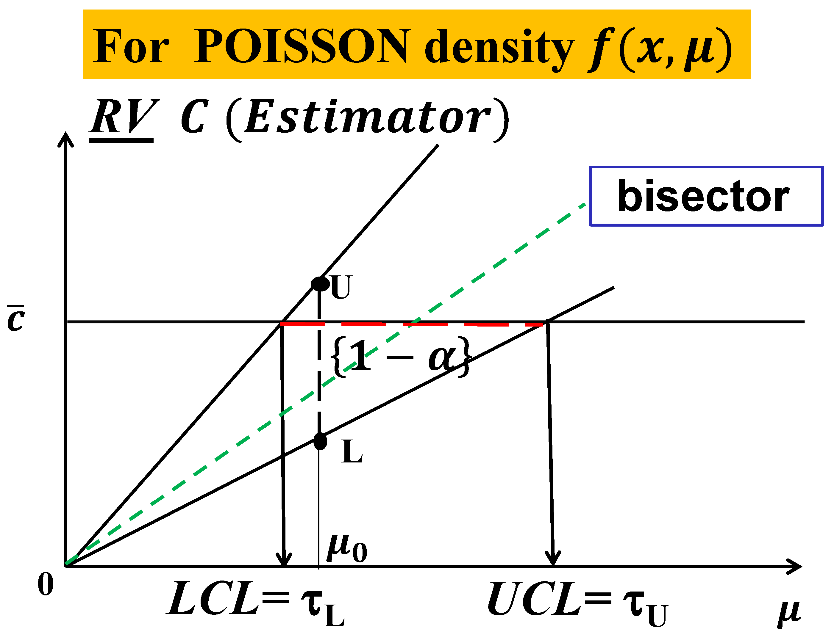
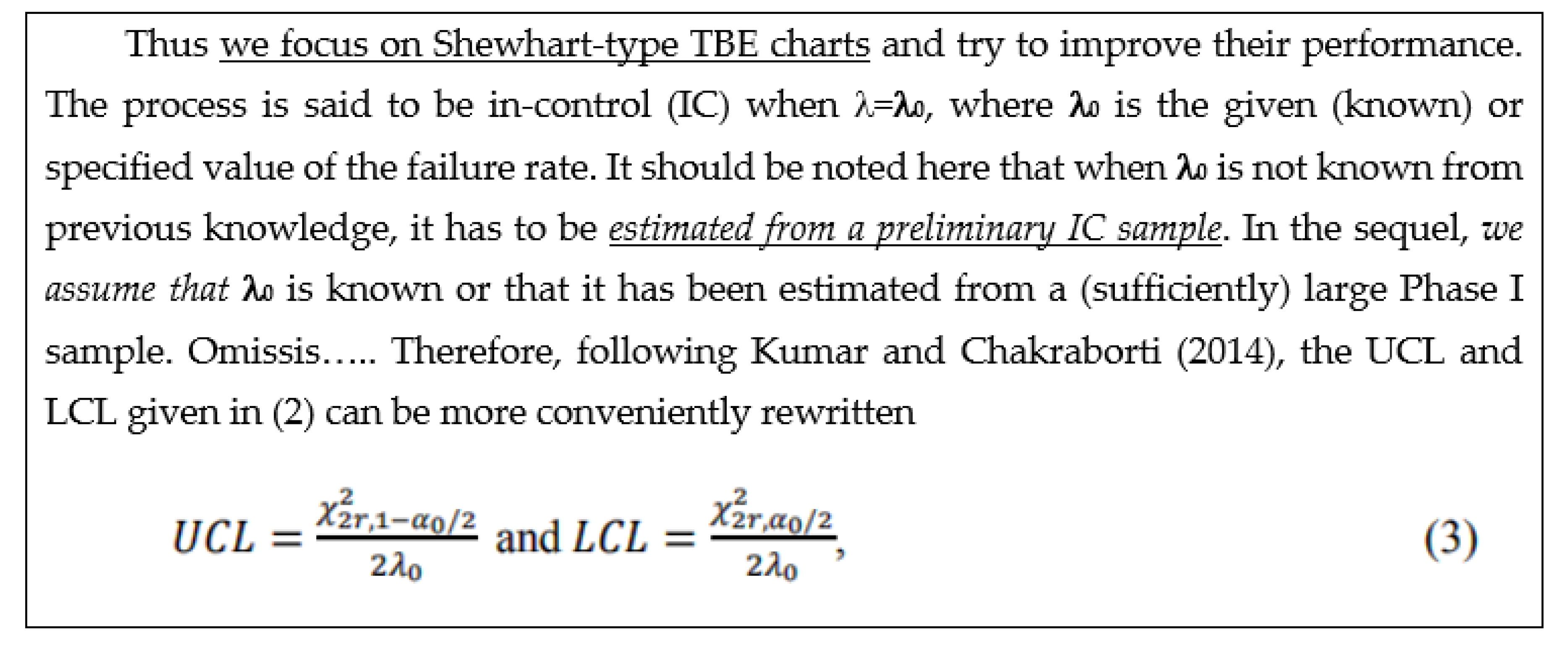
The practical problem, for TBE data (Exponentially ditsributed)” becomes hence a Theoretical one [1,2,3,4,5,6,7,8,9,10,11,12,13,14,15,16,17,18,19,20,21,22,23,24,25,26,27,28,29,30,31,32,33,34,35,36,37,38,39,40,41,42,43,44,45,46] (all references and Figure 1): we show here, immediately, the wrong formulae (either using the parameter or its estimate , with ) in the formula (1)
In the formulae (1), in the (named) interval LCL------UCL (Control Interval), the LCL must be L and the UCL must be U, vertical interval L------U (Figure 1); the actual interval LCL------UCL is the horizontal one in the Figure 1, which is not that of the formulae (1). Since the errors have been continuing for at least 25 years, we dare to say that this paper is an Education Advance for all the Scholars, for the software sellers and the users: they should study the books and papers in [1,2,3,4,5,6,7,8,9,10,11,12,13,14,15,16,17,18,19,20,21,22,23,24,25,26,27,28,29,30,31,32,33,34,35,36,37,38,39,40,41,42,43,44,45,46].
The readers could think that the I-CCs are well known and well dealt in the scientific literature about Quality. We have some doubt about that: we will show that, at least in one field, the I-CC_TBE (with TBE, Time Between Event data) usage, it is not so: there are several published papers, in “scientific magazines and Journals (well appreciated by the Scholars)” with wrong Control Limits; a sample of the involved papers (from 1994 to January 2024) can be found in [23,24]”. Therefore, those authors do not extract the maximum information from the data in the Process Control. “The Garden…” [24] and the excerpts 1, with the Deming’s statements, constitute the Literature Review.
We hope that the Deming statements about knowledge will interest the Readers (Excerpt 2).
A preliminary case is shown in Appendix A.
2. Materials and Methods
2.1. A Reduced Background of Statistical Concepts
This section is essential to understand the “problems related to Control Charts” as we found in the literature. We suggest it for the formulae given and for the difference between the concepts of PI (Probability Interval, NOT “Prediction Interval”, asd interpreted by a Peer Reviewer!) and CI (Confidence Interval): this is overlooked in “The Garden … [24]” (a sample of it is in the Appendix C).
See a first case in the appendix A. Therefore, we humbly ask the reader to carefully meditate on the content.
Engineering Analysis is related to the investigation of phenomena underlying products and processes; the analyst can communicate with the phenomena only through the observed data, collected with sound experiments (designed for the purpose): any phenomenon, in an experiment, can be considered as a measurement-generating process [MGP, a black box that we do not know] that provides us with information about its behaviour through a measurement process [MP, known and managed by the experimenter], giving us the observed data (the “message”).
It is a law of nature that the data are variable, even in conditions considered fixed, due to many unknown causes.
MGP and MP form the Communication Channel from the phenomenon to the experimenter.
The information, necessarily incomplete, contained in the data, has to be extracted using sound statistical methods (the best possible, if we can). To do that, we consider a statistical model F(x|θ) associated with a random variable (RV) X giving rise to the measurements, the “determinations” {x1, x2, …, xn}=D of the RV, constituting the “observed sample” D; n is the sample size. Notice the function F(x|θ) [a function of real numbers, whose form we assume we know] with the symbol θ accounting for an unknown quantity (or some unknown quantities) that we want to estimate (assess) by suitably analysing the sample D.
We indicate by the pdf (probability density function) and by the Cumulative Function, where is the set of the parameters of the functions.
When we have the Normal model, written as (x|), with (parameters) mean E[X]=μ and variance Var[X]=σ2
When we have Exponential model, with (the single parameter) mean E[X]= and variance Var[X]=2, written in two equivalent ways .
When we have Poisson model, with (the single parameter) mean E[X]= and variance Var[X]=, written as , with x=0, 1, 2, …., n, …
When we have the observed sample D={x1, x2, …, xn}, our general problem is to estimate the value of the parameters of the model (representing the parent population) from the information given by the sample. We define some criteria which we require a “good” estimate to satisfy and see whether there exist any “best” estimates. We assume that the parent population is distributed in a form, the model, which is completely determinated but for the value θ0 of some parameter, e.g. unidimensional, θ, or bidimensional θ={μ, σ2}; we consider only one or two parameters, for easiness.
We seek some function of θ, say τ(θ), named inference function, and we see if we can find a RV T which can have the following properties: unbiasedness, sufficiency, efficiency. Statistical Theory allows us the analysis of these properties of the estimators (RVs).
We use the symbols and for the unbiased estimators T1 and T2 of the mean and the variance.
Luckily, we have that T1, in the Exponential model and Poisson model , is efficient [6,7,8,9,10,11,12,13,14,15,16,17,18,19,20,21,25,26,27,28,29,30,31,32,33], and it extracts the total available information from any random sample, while the couple T1 and T2, in the Normal model, are jointly sufficient statistics for the inference function τ(θ)=(μ, σ2), so extracting the maximum possible of the total available information from any random sample. The estimators (which are RVs) have their own “distribution” depending on the parent model F(x|θ) and on the sample D: we use the symbol for that “distribution”. It is used to assess their properties. For a given (collected) sample D the estimator provides a value t (real number) named the estimate of τ(θ), unidimensional.
A way of finding the estimate is to compute the Likelihood Function [LF] and to maximise it: the solution of the equation =0 is termed Maximum Likelihood Estimate [MLE].
The LF is important because it allows us finding the MVB (Minimum Variance Bound, Cramer-Rao theorem) [1,2,6,7,8,9,10,11,12,13,14,15,16,26,27,28,29,30,31,32,33,34,35,36] of an unbiased RV T [related to the inference function τ(θ)], such that
The inverse of the MVB(T) provides a measure of the total available amount of information in D, relevant to the inference function τ(θ) and to the statistical model F(x|θ).
Naming IT(T) the information extracted by the RV T we have that [6,7,8,9,10,11,12,13,14,15,16,17,18,19,20,21,26,27,28,29,30,31,32,33,34,35,36]
IT(T)=1/MVB(T) ⇔ T is an Efficient Estimator.
If T is an Efficient Estimator there is no better estimator able to extract more information from D.
The estimates considered before were “point estimates” with their properties, looking for the “best” single value of the inference function τ(θ).
We must now introduce the concept of Confidence Interval (CI) and Confidence Level (CL) [6,7,8,9,10,11,12,13,14,15,16,17,18,19,20,21,26,27,28,29,30,31,32,33,34,35,36]. This point is very important for all the Control Charts: it was overlooked by thoousands of authors, Peer Reviers and Editors…
The “interval estimates” comprise all the values between τL (Lower confidence limit) and τU (Upper confidence limit); the CI is defined by the numerical interval CI={τL-----τU}, where τL and τU are two quantities computed from the observed sample D: when we make the statement that τ(θ)∈CI, we accept, before any computation, that, doing that, we can be right, in a long run of applications, (1-α)%=CL of the applications, BUT we cannot know IF we are right in the single application (CL=Confidence Level).
We know, before any computation, that we can be wrong α% of the times but we do not know when it happens.
The reader must be very careful to distinguish between the Probability Interval PI={L-----U}, where the endpoints L and U depends on the distribution of the estimator T (that we decide to use, which does not depend on the “observed sample” D) and, on the probability π=1-α (that we fix before any computation), as follows by the probabilistic statement (4) [se the Figure 1 for the exponential density, when n=1]
and Confidence Interval CI={τL-----τU} which depends on the “observed sample” D.
Notice that the Probability Interval PI={L-----U} does not depend on the data D: L and U are the Probability Limits. Notice that, on the contrary, the Confidence Interval CI={τL-----τU} does depend on the data D.
Shewhart identified this approach, L and U, on page 275 of [19] where he states:
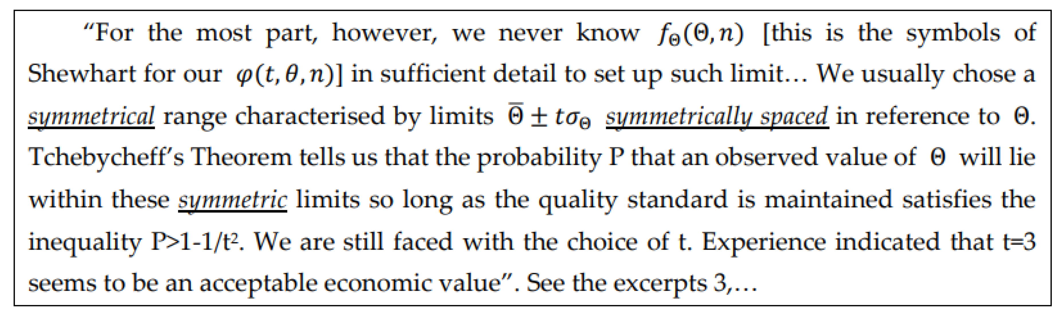
The Tchebycheff Inequality: IF the RV X is arbitrary with density f(x) and finite variance THEN we have the probability , where . This is a “Probabilistic Theorem”.
It can be transferred into Statistics. Let’s suppose that we want to determine experimentally the unknown mean within a “stated error ε“. From the above (Probabilistic) Inequality we have ; IF THEN the event is “very probable” in an experiment: this means that the observed value of the RV X can be written as and hence . In other words, using as an estimate of we commit an error that “most likely” does not exceed . IF, on the contrary, , we need n data in order to write , where is the RV “mean”; hence we can derive ., where is the “empirical mean” computed from the data. In other words, using as an estimate of we commit an error that “most likely” does not exceed . See the excerpts 3, 3a, 3b.
Notice that, when we write , we consider the Confidence Interval CI [6,7,8,9,10,11,12,13,14,15,16,17,18,19,20,21,25,26,27,28,29,30,31,32,33], and no longer the Probability Interval PI [6,7,8,9,10,11,12,13,14,15,16,17,18,19,20,21,25,26,27,28,29,30,31,32,33].
These statistical concepts are very important for our purpose when we consider the Control Charts, especially the Individual CCs, I-CC.
Notice that the error made by several authors [3,4,5,24] is generated by lack of knowledge of the difference between PI and CI [6,7,8,9,10,11,12,13,14,15,16,17,18,19,20,21,25,26,27,28,29,30,31,32,33]: they think wrongly that CI=PI, a diffused disease [3,4,5,24]! They should study some of the books/papers [6,7,8,9,10,11,12,13,14,15,16,17,18,19,20,21,25,26,27,28,29,30,31,32,33] and remember the Deming statements (Excerpt 2).
The Deming statements are important for Quality. Managers, scholars; the professors must learn Logic, Design of Experiments and Statistical Thinking to draw good decisions. The authors must, as well. Quality must be their number one objective: they must learn Quality methods as well, using Intellectual Honesty [1,2,6,7,8,9,10,11,12,13,14,15,16,17,18,19,20,21,25,26,27,28,29,30,31,32,33]. Using (4), those authors do not extract the maximum information from the data in the Process Control. To extract the maximum information from the data one needs statistical valid Methods [1,2,6,7,8,9,10,11,12,13,14,15,16,17,18,19,20,21,25,26,27,28,29,30,31,32,33].
As you can find in any good book or paper [6,7,8,9,10,11,12,13,14,15,16,17,18,19,20,21,25,26,27,28,29,30,31,32,33] there is a strict relationship between CI and Test Of Hypothesis, known also as Null Hypothesis Significance Testing Procedure (NHSTP). In Hypothesis Testing, the experimenter wants to assess if a “thought” value of a parameter of a distribution is confirmed (or rejected) by the collected data: for example, for the mean μ (parameter) of the Normal (x|) density, he sets the “null hypothesis” H0={μ=μ0} and the probability P=α of being wrong if he decides that the “null hypothesis” H0 is true, when actually it is opposite: H0 is wrong. We analyse the observed sample D={x1, x2, …, xn} and we compute the empirical (observed) mean and the empirical (observed) standard deviation hence, we define the Acceptance interval, which is the CI
Notice that the following interval (for the Normal model) [see the appendix B]
is the Probability Interval such that , and NOT the Confidence Interval and thus NOT the LCL------UCL (for the CCs).
A fundamental reflection is in order: the formulae (5) and (6) tempt the unwise guy to think that he can get the Acceptance interval, which is the CI [1,2,3,4,5,6,7,8,9,10,11,12,13,14,15,16,17,18,19,20,21,22,23], by substituting the assumed values of the parameters with the empirical (observed) mean and standard deviation . This trick is valid only for the Normal distribution.
In the field of Control Charts, following Shewhart, instead of the formula (5), we use (7)
where the value of the t distribution is substituted by the value of the Normal distribution, actually =3, and a coefficient is used to make “unbiased” the estimate of the standard deviation, computed from the information given by the sample.
Actually, Shewhart himself does not use the coefficient is as you can see from page 294 of Shewhart book (1931), where is the “Grand Mean”, computed from D [named here empirical (observed) mean ], is “estimated standard of each sample” (named here s, with sample size n=20, in Excerpt 3)
The application of these ideas in the Individual CCs can be seen in the Appendix A, in the Figure A1: the standard deviation is derived from the Mobile Range (which is exponentially distributed as the original UTI data). The formula in the Excerpt 3 tells us that the process is OOC (Out Of Control).
2.2. Control Charts for Process Management
Statistical Process Management (SPM) entails Statistical Theory and tools used for monitoring any type of processes, industrial or not. The Control Charts (CCs) are the tool used for monitoring a process, to assess its two states: the first, when the process, named IC (In Control), operates under the common causes of variation (variation is always naturally present in any phenomenon) and the second, named OOC (Out Of Control), when the process operates under some assignable causes of variation. The CCs, using the observed data, allow us to decide if the process is IC or OOC. CCs are a statistical test of hypothesis for the process null hypothesis H0={IC} versus the alternative hypothesis H1={OOC}. Control Charts were very considered by Deming [9,10] and Juran [12] after Shewhart invention [19,20].
We start with Shewhart ideas (see the excerpts 3, 3a and 3b).
Excerpt 3a.
From Shewhart book (1931), on page 89.
In the excerpts, is the (experimental) “Grand Mean”, computed from D (we, on the contrary, use the symbol ), is the (experimental) “estimated standard of each sample” (we, on the contrary, use the symbol s, with sample size n=20, in excerpts 3a, 3b), is the “estimated mean standard deviation of all the samples” (we, on the contrary, use the symbol ).
On page 95, he also states that
Excerpt 3b.
From Shewhart book (1931), on page 294.
So, we clearly see that Shewhart, the inventor of the CCs, used the data to compute the Control Limits, LCL (Lower Control Limit) and UCL (Upper Control Limit) both for the mean (the 1st parameter of the Normal pdf) and for (the 2nd parameter of the Normal pdf). They are considered the limits comprising 0.9973n of the observed data. Similar ideas can be found in [5,6,7,8,9,10,11,12,13,14,15,16,17,18,19,20,21,25,26,27,28,29,30,31,32,33,34,35,36,37,38,39,40,41,42] (with Rozanov, 1975, we see the idea that CCs can be viewed as a Stochastic Process).
We invite the readers to consider that if one assumes that the process is In Control (IC) and if he knows the parameters of the distribution he can test if the assumed known values of the parameters are confirmed or disproved by the data, then he does not need the Control Charts; it is sufficient to use NHSTP! (see App. B)
Remember the ideas in the previous section and compare Excerpts 3, 3a, 3b (where LCL, UCL depend on the data) with the following Excerpt 4 (where LCL, UCL depend on the Random Variables) and appreciate the profound “logic” difference: this is the cause of the many errors in the CCs for TBE [Time Between Events (see [4,5,24]).
The formulae, in the Excerpt 4, LCL1 and UCL1 are actually the Probability Limits (L and U) of the Probability Interval PI in the formula (4), when is the pdf of the Estimator T, related to the Normal model F(x; μ, σ2). Using (4), those authors do not extract the maximum information from the data in the Process Control. From the Theory [6,7,8,9,10,11,12,13,14,15,16,17,18,19,20,21,22,23,24,25,26,27,28,29,30,31,32,33,34,35,36] we derive that the interval L=μY-3σY------μY+3σY=U is the PI such that the RV Y=
and it is not the CI of the mean μ=μY [as wrongly said in the Excerpt 4, where actually (LCL1-----UCL1)=PI].
The same error is in other books and papers (not shown here but the reader can see in [21,22,23,24]).
The data plotted in the CCs [6,7,8,9,10,11,12,13,14,15,16,17,18,19,20,21,25,26,27,28,29,30,31,32,33,34,35,36] (see the Figure 2) are the means , determinations of the RVs , i=1, 2, ..., n (n=number of the samples) computed from the collected data of the i-th sample Di={xij, j=1, 2, ..., k} (k=sample size)}, determinations of the RVs at very close instants tij, j=1, 2, ..., k. In other applications I-CC (see the Figure 3), the data plotted are the Individual Data , determinations of the Individual Random Variables , i=1, 2, ..., n (n=number of the collected data), modelling the measurement process (MP) of the “Quality Characteristic” of the product: this model is very general because it is able to consider every distribution of the Random Process , as we can see in the next section. From the excerpts 3, 3a, 3b and formula (5) it is clear that Shewhart was using the Normal distribution, as a consequence of the Central Limit Theorem (CLT) [6,7,8,9,10,11,12,13,14,15,16,17,18,19,20,26,27,28,29,30,31,32,33,34,35,36]. In fact, he wrote on page 289 of his book (1931) “… we saw that, no matter what the nature of the distribution function of the quality is, the distribution of the arithmetic mean approaches normality rapidly with increase in n (his n is our k), and in all cases the expected value of means of samples of n (our k) is the same as the expected value of the universe” (CLT in Excerpt 3, 3a, 3b).
Let k be the sample size; the RVs are assumed to follow a normal distribution and uncorrelated; [ith rational subgroup] is the mean of RVs IID j=1, 2, ..., k, (k data sampled, at very near times tij).
To show our way of dealing with CCs we consider the process as a “stand-by system whose transition times from a state to the subsequent one” are the collected data. The lifetime of “stand-by system” is the sum of the lifetimes of each unit. The process (modelled by a “stand-by …”) behaves as a Stochastic Process [25,26,27,28,29,30,31,32,33], that we can manage by the Reliability Integral Theory (RIT): see the next section; this method is very general because it is able to consider every distribution of .
If we assume that is distributed as f(x) [probability density function (pdf) of “transitions from a state to the subsequent state” of a stand-by subsystem] the pdf of the (RV) mean is, due the CLT (page 289 of 1931 Shewhart book), [experimental mean ] with mean and variance . is the “grand” mean and is the “grand” variance: the pdf of the (RV) grand mean [experimental “grand” mean ]. In Figure 2 we show the determinations of the RVs and of .
When the process is Out Of Control (OOC, assignable causes of variation, some of the means , estimated by the experimental means , are “statistically different)” from the others [6,7,8,9,10,11,12,13,14,15,16,17,18,19,20,21,25,26,27,28,29,30,31,32,33,34,35,36]. We can assess the OOC state of the process via the Confidence Interval (provided by the Control Limits) with CL=0.9973; see the Appendix B. Remember the trick valid only for the Normal Distribution ….; consider the PI, L=μY-3σY------μY+3σY=U; putting in place of and in place of we get the CI of when the sample size k is considered for each , with CL=0.9973. The quantity is the mean of the standard deviations of each sample. This allows us to compare each (subsystem) mean , q=1,2, …, n, to any other (subsystem) mean r=1,2, …, n, and to the (Stand-by system) grand mean . If two of them are different, the process is classified as OOC. The quantities and are the Control Limits of the CC. When the Ranges Ri=max(xij)-min(xij) are considered for each sample we have , and , U, where is the “mean range” and the coefficients A2, D3, D4 are tabulated and depend on the sample size k [6,7,8,9,10,11,12,13,14,15,16,17,18,19,20,21,25,26,27,28,29,30,31,32,33,34,35,36].
See the Appendix B: it is important for understanding our ideas.
The interval LCLX-------UCLX is the “Confidence Interval” with “Confidence Level” CL=1-α=0.9973 for the unknown mean of the Stochastic Process X(t) [25,26,27,28,29,30,31,32,33,34,35,36]. The interval LCLR----------UCLR is the “Confidence Interval” with “Confidence Level” CL=1-α=0.9973 for the unknown Range of the Stochastic Process X(t) [25,26,27,28,29,30,31,32,33,34,35,36].
Notice that, ONLY for normally distributed data, the length of the Control Interval (UCLX-LCLX, which is the Confidence Interval) equals the length of the Probability Interval, PI (U-L): UCLX-LCLX=U-L.
The error highlighted, i.e. the confusion between the Probability Interval and the Control Limits (Confidence Interval!) has no consequences for decisions when the data are Normally distributed, as considered by Shewhart. On the contrary, it has BIG consequences for decisions WHEN the data are Non-Normally distributed [4,5,24].
We think that the paper “Quality of Methods for Quality is important”, [1] appreciated and mentioned by J. Juran at the plenary session of the EOQC (European Organization for Quality Control) Conference (1989), should be considered and meditated.
2.3. Control Charts for Attributes
We consider here the papers [3] and “Bayesian Control Chart for Number of Defects in Production Quality Control. Mathematics 2024. From the papers we read:
Excerpt 5.
From the a. m. papers.
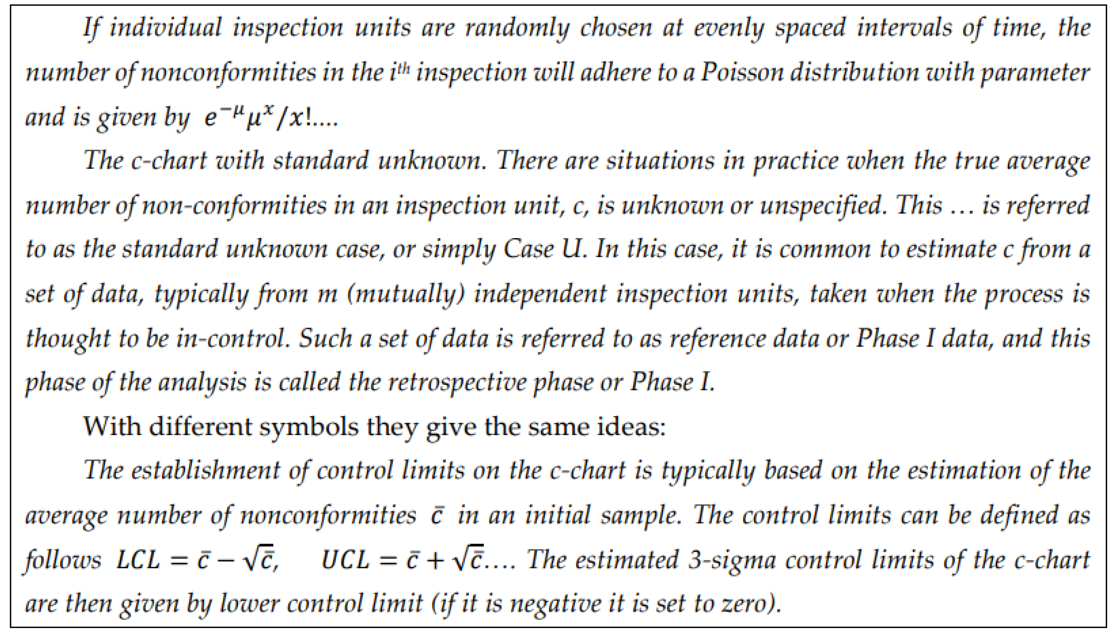
Since we know that for the Poisson model, we have mean E[X]= and variance Var[X]=, it is clear that the Control Limits , are exactly the same for the Normal distribution (seen above, with k=1, and ), assuming the validity of the CLT (Central Limit Theorem), so that we could write the probability statement … It is easily seen that LCL and UCL are obtained by puggling in for in the previous probability statement.
This is Theoretically Wrong. We name tis the “classical” method.
As a matter of fact, letting C be the RV “number of Nonconforming in a sample” (Estimator) and the “estimate (grand mean)” of the mean from the Theory (6-46) we derive the Figure 1b. Thus LCL----UCL ≠ L----U (Probability interval).
Figure 1b.
Control Limits for the c Chart. LCL----UCL ≠ L----U (Probability interval) “grand mean”
The error implied in the Chakraborti Control Limits formula is repeated by that author in several other papers on CCs for Exponential distribution [24] (see later).
To illustrate its ideas Chakraborti consider an example (7.3 from Montgomery book 8th ed.). A total of 26 successive inspection samples (consisting of 100 individual units of product) were considered in Phase I to estimate c. Since in this phase 2 samples were OOC they were discarded and then 24 were the samples for the Control Limits. The estimate is and using the “wrong formulae” LCL1=6.36 and UCL1=32.97; on the contrary, usign the the Theory (Figure 1b) we got LCL2=9.19 and UCL2=36.10; our result, in Figure 4, show the different Control Limits with other 20 new samples were collected for Phase II: Chakraborti and Montgomery conclude “No lack of control is indicated.”.
Figure 4 says the opposite: the sample 44 is OOC.
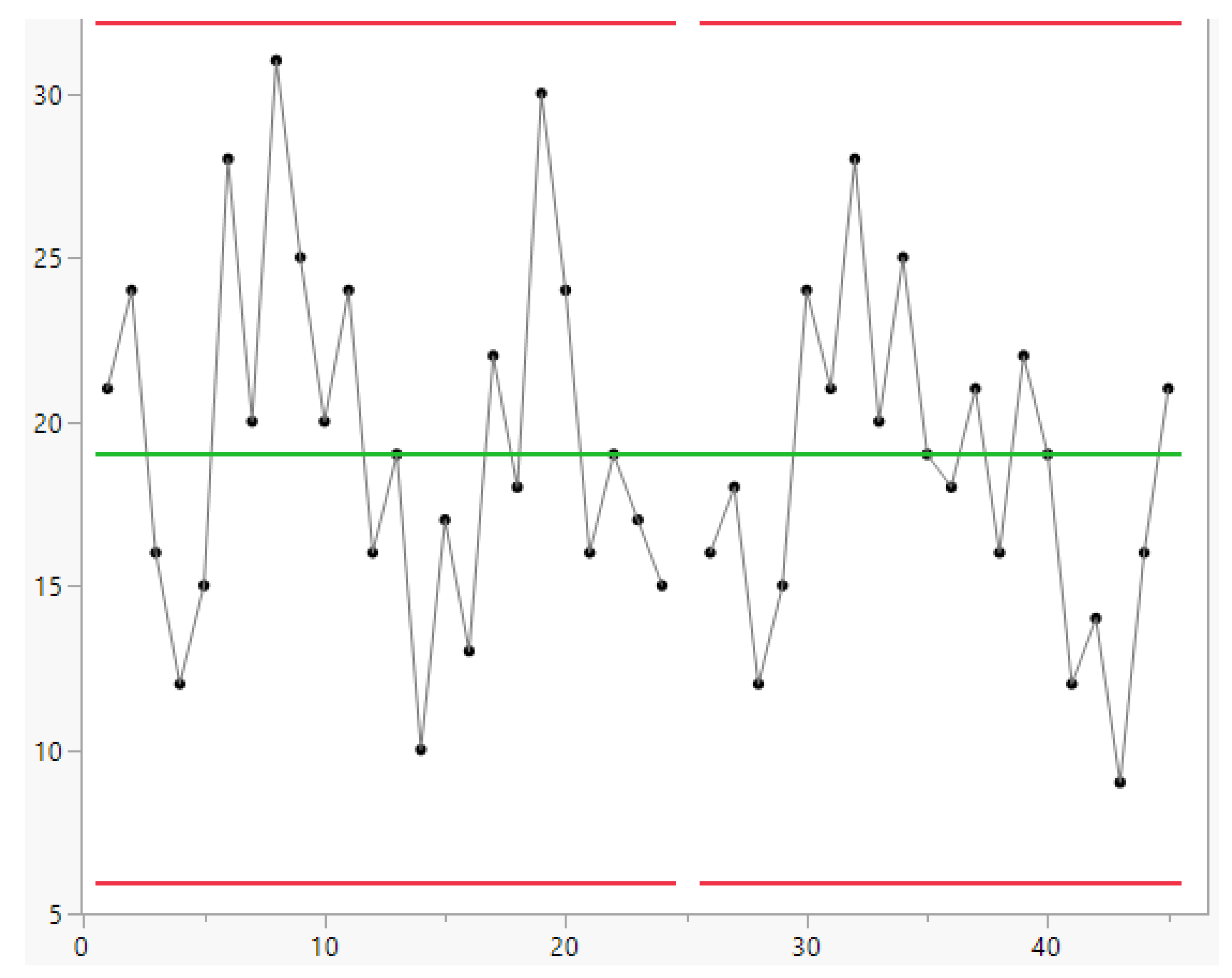
Notice that the statitical software JMP does not find the OOC (see the Figure 4b), because it uses the “wrong formulae”.
We caried out several “10000 simulations” with various μ to check LCL1 and UCL1 versus LCL2 and UCL2; the result is clear: The “classical” method misses real OOC and finds non-existent OOC.
Therefore it is clear that authors, Peer Reviewers and Editors should use the Thoery to analyse the “Scientificness” of papers.
Figure 4.
Control Limits (by FG) for the c Chart of the Montgomery case.
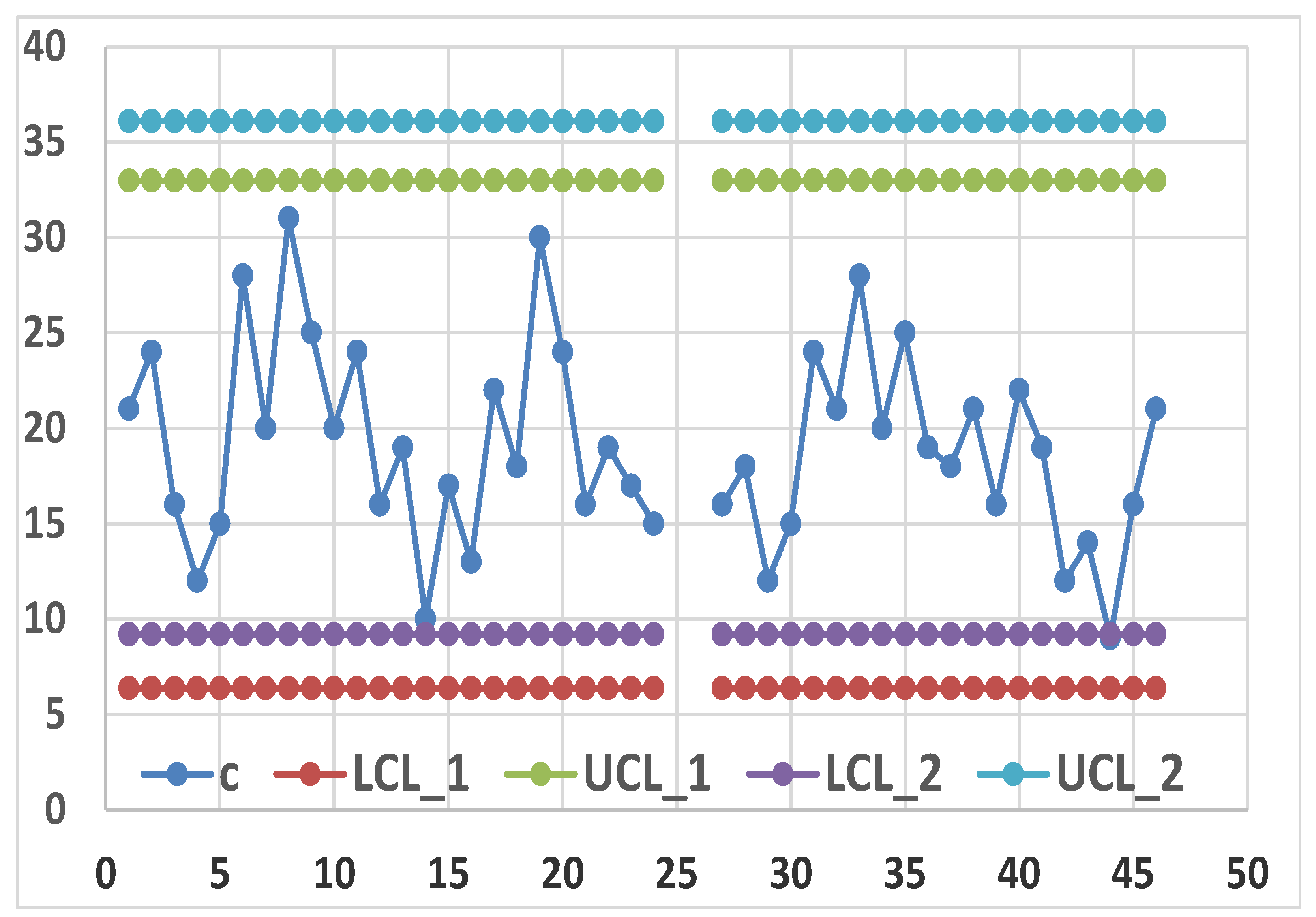
Figure 4b.
Control Limits (by JMP) for the c Chart of the Montgomery case.
2.4. Statistics and RIT
We are going to present the fundamental concepts about RIT (Reliability Integral Theory) that we use for computing the Control Limits of CCs. RIT can be found in the author’s books…
RIT can be used for parameters estimation and Confidence Intervals (CI), (Galetto 1981, 1982, 1995, 2010, 2015, 2016), in particular for Control Charts (Deming, 1986, 1997, Shewhart 1931, 1936, Galetto 2004, 2006, 2015). In fact, any Statistical or Reliability Test can be depicted by an “Associated Stand-by System” [25,26,27,28,29,30,31,32,33,34,35,36] whose transitions are ruled by the kernels bk,j(s); we write the fundamental system of integral equations for the reliability tests, whose duration t is related to interval 0-----t; the collected data tj can be viewed as the times of the various failures (of the units comprising the System) [t0=0 is the start of the test, t is the end of the test and g is the number of the data (4 in the Figure 4)]
Firstly, we assume that the kernel is the pdf of the exponential distribution (|), where is the failure rate of each unit and : is the MTTF of each unit. We state that is the probability that the stand-by system does not enter the state g (5 if we connsider 4 units), at time t, when it starts in the state j (0, 1, …, 4) at time tj, is the probability that the system does not leave the state j, is the probability that the system makes the transition j→j+1, in the interval s-----s+ds.
The system reliability is the solution of the mathematical system of the Integral Equations (8)
With we obtain the solution (see Figure 5, putting the Mean Time To Failure MTTF=θ=123 days, ); notice that it is 1-CDF (Poisson) with
The reliability system (8) can be written in matrix form,
At the end of the reliability test, at time t, we know the data (the times of the transitions tj) and the “observed” empirical sample D={x1, x2, …, xg}, where xj=tj – tj-1 is the length between the transitions; the transition instants are tj = tj-1 + xj giving the “observed” transition sample D*={t1, t2, …, tg-1, tg, t=end of the test} (times of the transitions tj).
We consider now that we want to estimate the unknown MTTF=θ=1/λ of each item comprising the “associated” stand-by system [24,25,26,27,28,29,30]: each datum is a measurement from the exponential pdf; we compute the determinant of the integral system (9), where is the “Total Time on Test” [ in the Figure 5]: the “Associated Stand-by System” [25,26,27,28,29,30,31,32,33] in the Statistics books provides the pdf of the sum of the RV Xi of the “observed” empirical sample D={x1, x2, …, xg}. At the end time t of the test, the integral equations, constrained by the constraintD*, provide the equation
It is important to notice that, in the case of exponential distribution [11,12,13,14,15,16,25,26,27,28,29,30,31,32,33,34,35,36], it is exactly the same result as the one provided by the MLM Maximum Likelihood Method.
If the kernel is the pdf (|) the data are normally distributed, , with sample size n, then we get the usual estimator such that .
The same happens with any other distribution provided that we write the kernel .
The reliability function , [formula (8)], with the parameter , of the “Associated Stand-by System” provides the Operating Characteristic Curve (OC Curve, reliability of the system) [6,7,8,9,10,11,12,13,14,15,16,17,18,19,20,21,22,23,24,25,26,27,28,29,30,31,32,33,34,35,36] and allows to find the Confidence Limits ( Lower and Upper) of the “unknown” mean , to be estimated, for any type of distribution (Exponential, Weibull, Rayleigh, Normal, Gamma, …); by solving, with unknown , the two equations (|); we get the two values (, ) such that
where is the (computed) “total of the length of the transitions xi=tj - tj-1 data of the empirical sampleD” and CL= is the Confidence Level. CI=-------- is the Confidence Interval: and .
For example, with Figure 5, we can derive and , with CL=0.8. It is quite interesting that the book [14] Meeker et al., “Statistical Intervals: A Guide for Practitioners and Researchers”, John Wiley & Sons (2017) use the same ideas of FG (shown in the formula 11) for computing the CI; the only difference is that the author FG defined the procedure in 1982 [26], 35 years before Meeker et al.
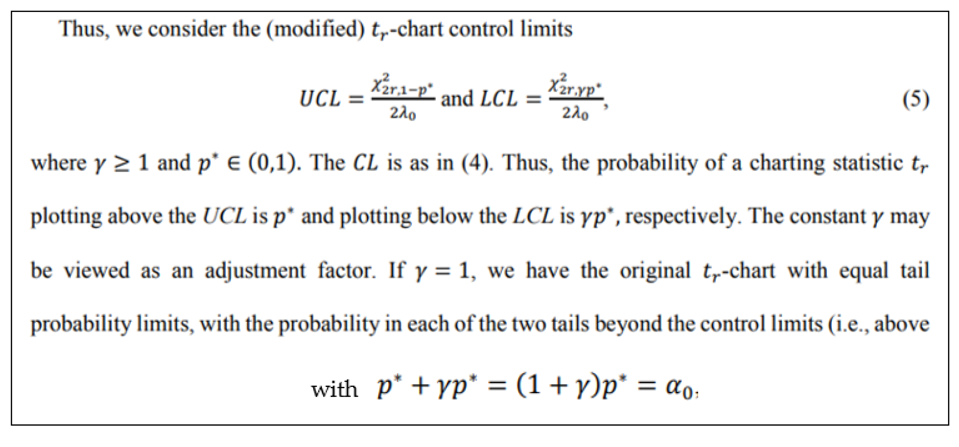
2.5. Control Charts for TBE Data. Some Ideas for Phase I Analysis
Let’s consider now TBE (Time Between Event) data, exponentially or Weibull distributed. Quite a lot of authors (in the “Garden … [24]”) compute wrongly the Control Limits of these CCs.
The formulae, shown in the section “Control Charts for Process Management”, are based on the Normal distribution (thanks to the CLT; see the excerpts 3, 3a and 3b); unfortunately, they are used also for NON_normal data (e.g. see formulae (1)): for that, sometimes, the NON_normal data are transformed “with suitable transformations” in order to “produce Normal data” and to apply those formulae (above) [e.g. Montgomery in his book].
Sometimes we have few data and then we use the so called “Individual Control Charts” I-CC. The I-CCs are very much used for exponentially (or Weibull) distributed data: they are also named “rare events Control Charts for TBE (Time Between Events) data”, I-CC_TBE.
The Jarret data (1979) are used also in the paper (found online, 2024, March 1) [4] (Kumar, Chakraborti et al. with various presence in the “Garden … [24]”) who decided to consider the paper [5] (Zhang et al. also present in the “Garden …]”): they use the first 30 observed time intervals as phase 1 and start the monitoring at m = 31. You find the original data in the Table 1 in the paper [3]; moreover, for the benefit of the readers we provide them in the section 3 “Results”.
It is a very good example for understanding better the problem and the consequences of the difference between PI (Probability Intervals) and the Control Limits, using RIT.
Let’s see what the authors say: Kumar, Chakraborti et al. , Journal of Quality Technology, 2016, present the case by writing (highlight due to FG):
Excerpt 5.
From Kumar, Chakraborti et al., “Journal of Quality Technology”, 2016.
In the paper of Zhang et al. (2006) we read:
Excerpt 6.
From Zhang et al. (2006), “IIE Transactions”.
Zhang et al., 2006, compute the Control Limits from the first 30 data and find LCL=0.268 and UCL=1013.9 (you can see them in their Table 7, that is “our” Excerpt 11).
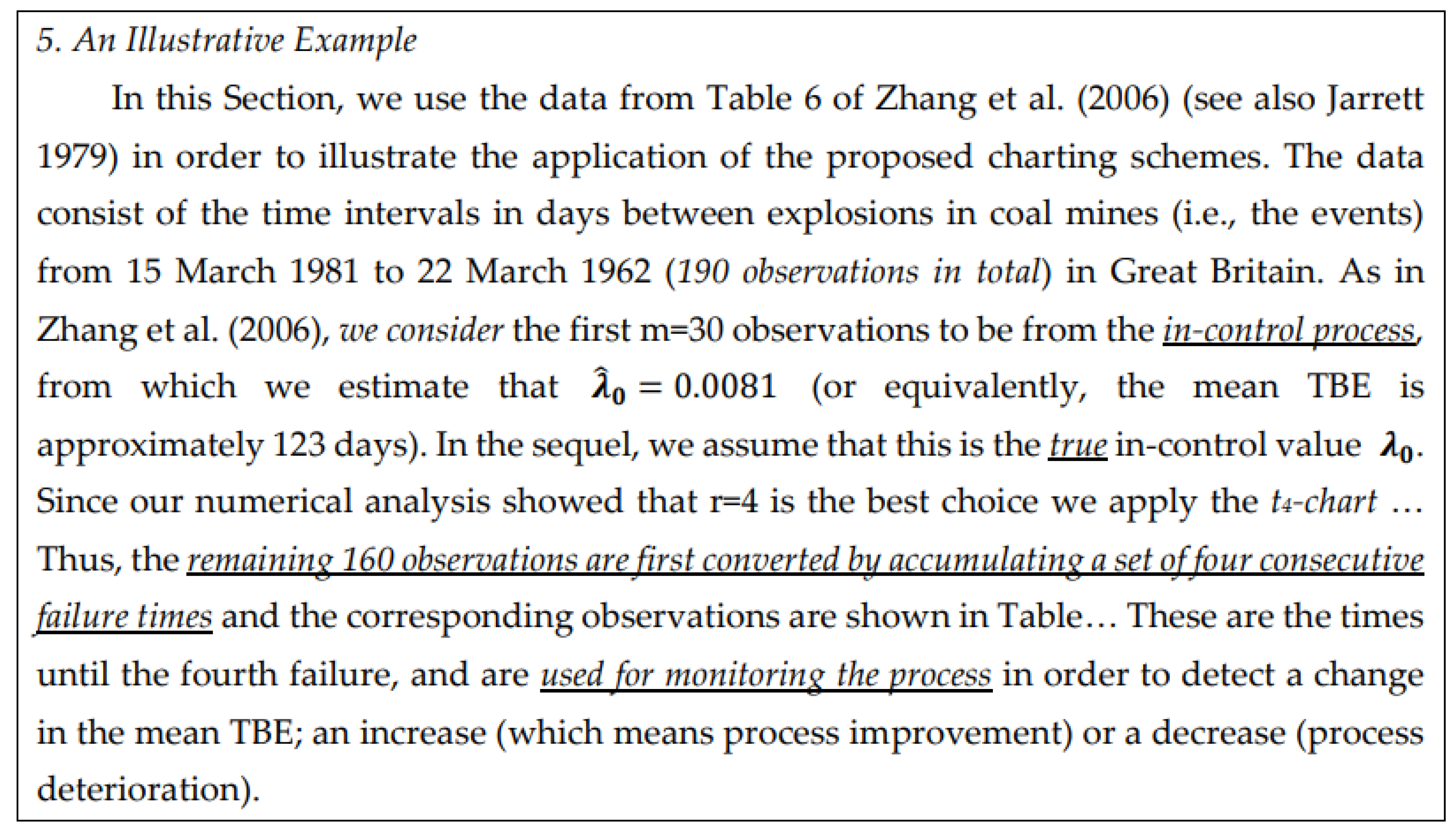
All the data [30+40 t4] are very interesting for our analysis; we recap the two important points, given by the authors (Kumar et al.):
- … first m=30 observations to be from the in-control process, from which we estimate … the mean TBE approximately, 123 days; we name it θ0.
- … we apply the t4-chart… Thus, … converted by accumulating a set of four consecutive failure times … the times until the fourth failure, used for monitoring the process to detect a change in the mean TBE.
The 3 authors (Kumar, Chakraborti et al.) state: “… the control limits … t4-chart are seen to be equal to LCL=63.95, UCL=1669.28 with CL (Centre Line)=451.79.”
Notice that the authors Zhang et al. and Kumar, Chakraborti et al. find different Control Limits to be used for monitoring the same process: a very interesting situation; the reason is that they use “different” statistics in Phase II.
The FG findings for the Phase I, using the first 30 data, compute different Control Limits with RIT: RIT solves the I-CC_TBE with exponentially distributed data as those of Table 1, considered by Zhang et al. and Kumar et al.
In the previous section, we computed the CI=-------- of the parameter , using the (subsample) “transition times durations”: =“total of the transition times durations (length of the transitions xi=tj - tj-1 data) in the empirical sample (subsample with n=4 only, as an example)” and Confidence Level CL=.
When we deal with a I-CC_TBE we compute the LCL and UCL of the mean θ through the empirical mean of each transition, for the n=30 data (Phase I of Zhang et al. and Kumar et al.); we solve the two following equations (12) for the two unknown values LCL and UCL, for of each item in the sample, similar to (11)
where now /n is the “mean, to be attributed, to the single lengths of the single transitions xi=tj-tj-1 data in the empirical sample D with the Confidence Level CL=: and .
In the next sections we can see the Scientific Results found by a Scientific Theory (we anticipate them: the Control Limits are LCL=18.0 days and UCL=88039.3 days).
3. Results
In these sections we provide the scientific analysis of the Jarret data [3] and compare our result with those of Chakraborty [4,5]: the findings are completely different and the decisions, consequently, should be different, with different costs of wrong decisions.
3.1. Control Charts for TBE Data. Phase I Analysis
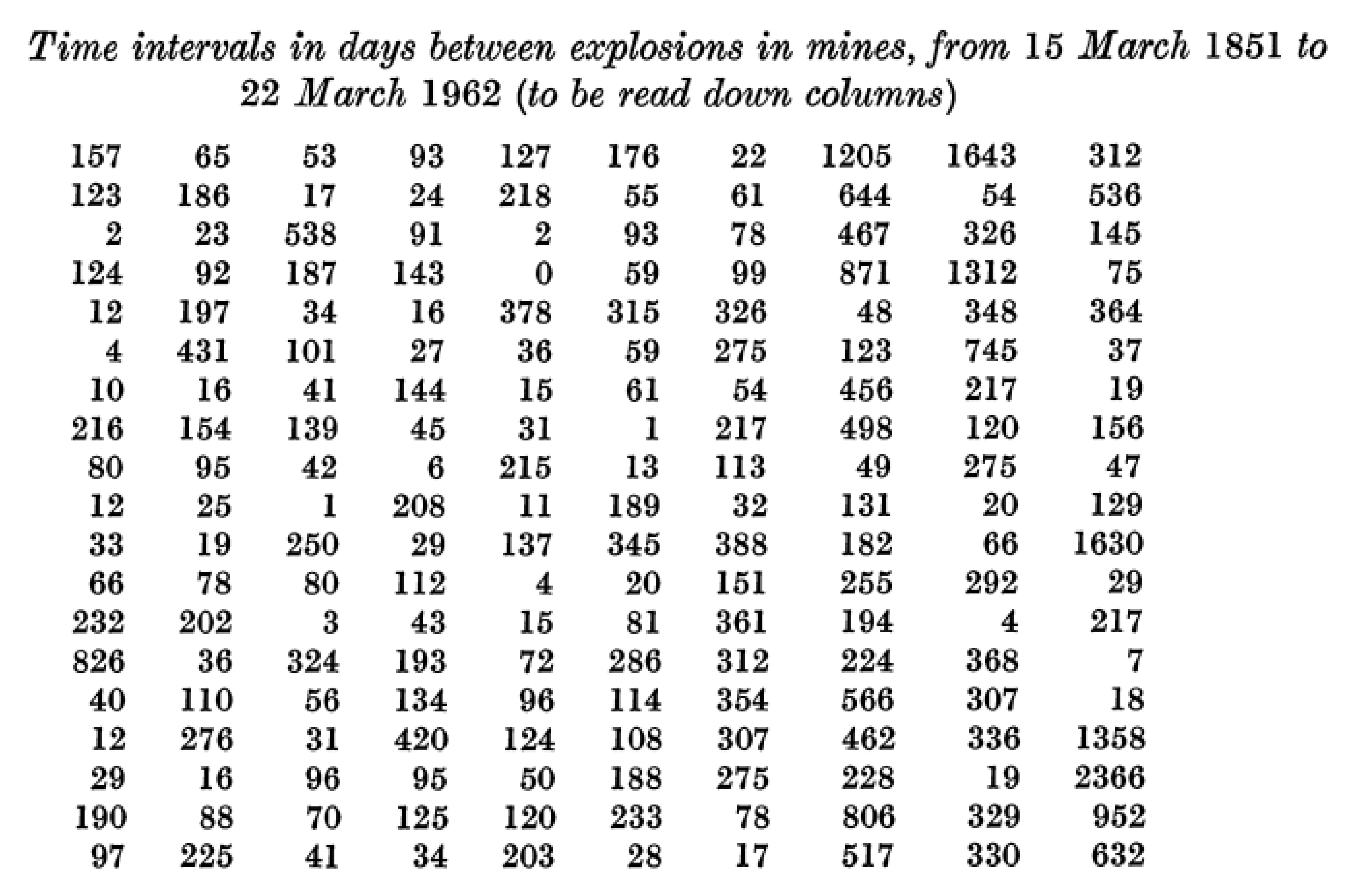
The Jarret data are in the Table 1.

Table 1.
Data from “A Note on the Intervals Between Coal-Mining Disasters”, Biometrika (1979).
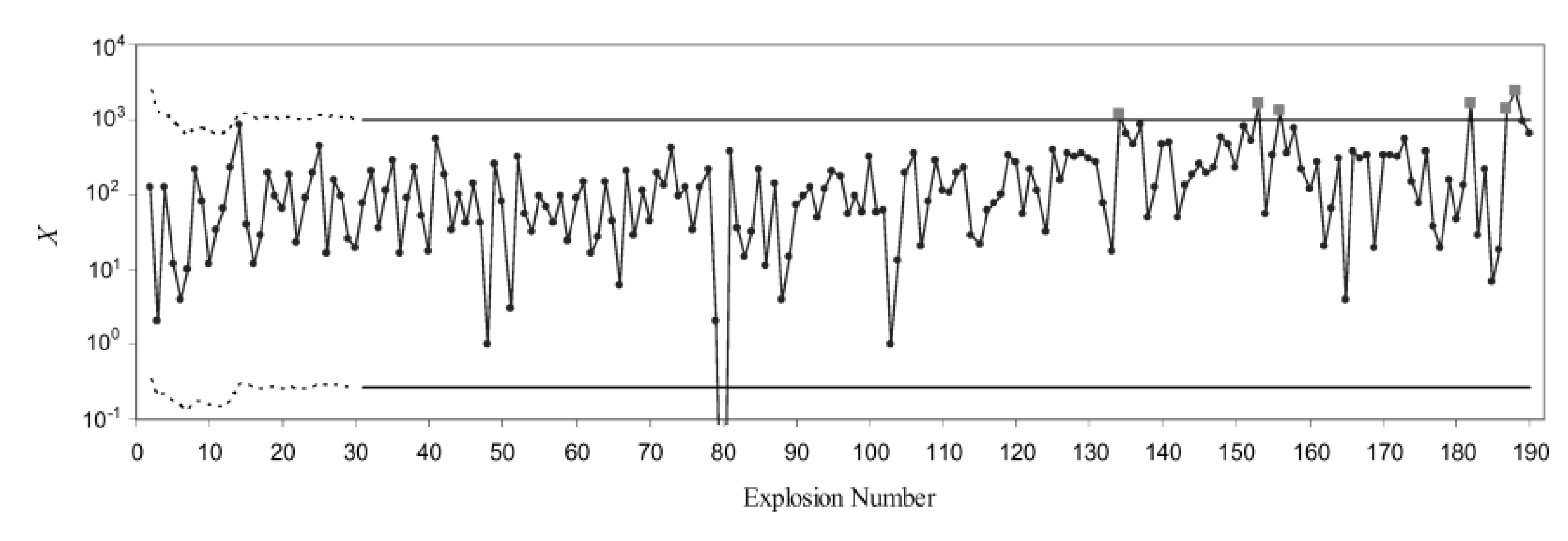
Excerpt 7.
The CC of the 190 data from “Improved Shewhart-Type Charts for Monitoring Times Between Events”, Journal of Quality Technology, 2016, (Kumar, Chakraborti et al): the first 30 are used to find the Control Limits for the other 40 t4 (time between “4 failures”: 4*40=160).
Excerpt 7.
The CC of the 190 data from “Improved Shewhart-Type Charts for Monitoring Times Between Events”, Journal of Quality Technology, 2016, (Kumar, Chakraborti et al): the first 30 are used to find the Control Limits for the other 40 t4 (time between “4 failures”: 4*40=160).
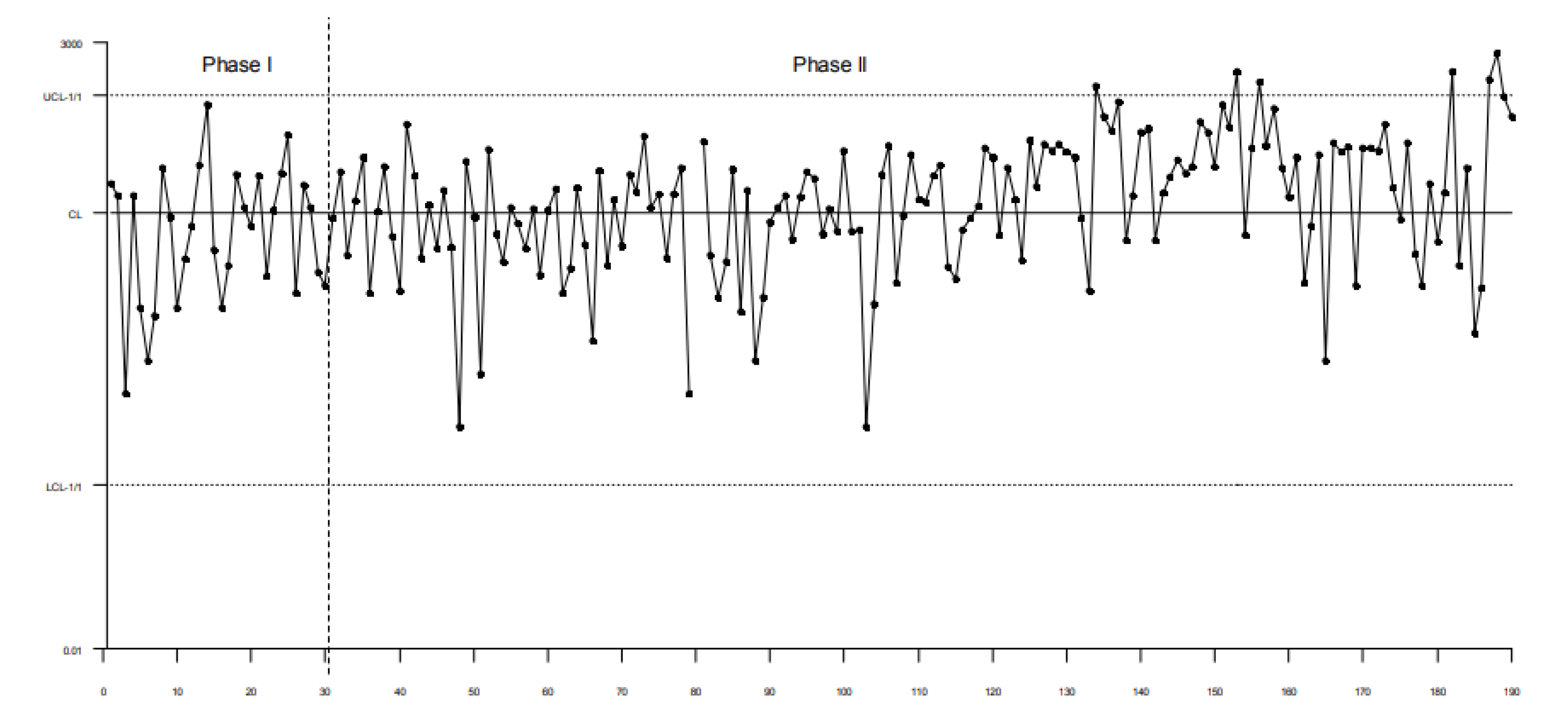
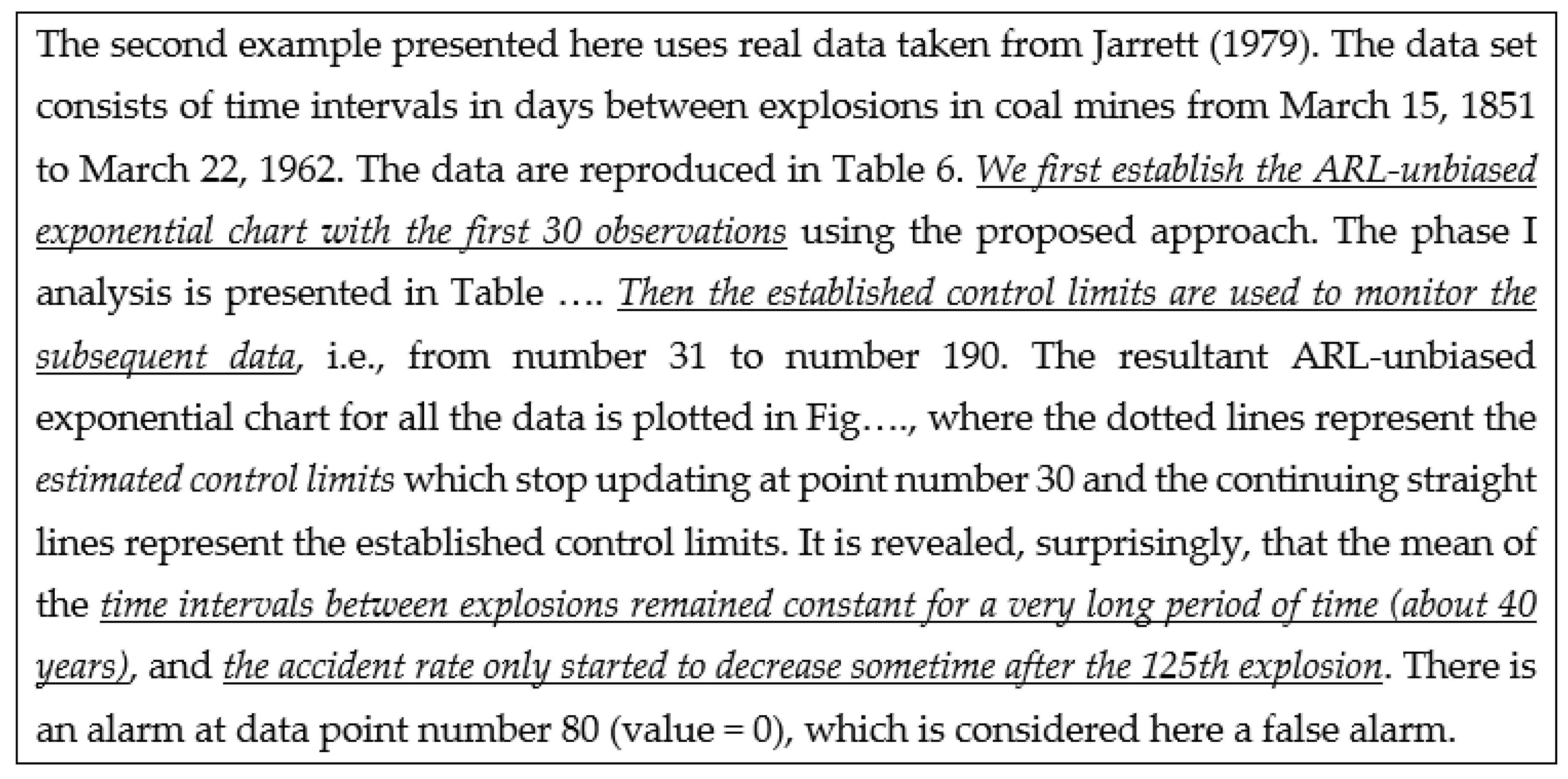
Excerpt 8.
The CC of the 190 data [named by the authors “ Figure 7. ARL-unbiased exponential chart for the coal mining data”] from “Design of exponential control charts using a sequential sampling scheme”, IIE Transactions, (Zhang et al., 2006) [the first 30 data are used to find the Control Limits].
Notice that the authors Zhang et al. and Kumar, Chakraborti et al. find different Control Limits to be used for monitoring the same process: a very interesting situation; the reason is that they use “different” statistics in Phase II. The results are in the excerpts 7 and 8.
For exponentially distributed data (12) becomes (13) [6,7,8,9,10,11,12,13,14,15,16,17,18,19,20,21,22,23,24,25,26,27,28,29,30,31,32,33], k=1, with CL=
The endpoints of the CI=--------are the Control Limits of the I-CC_TBE.
This is the right method to extract the “true” complete information contained in the sample (see theFigure 9).
The Figure 9 is justified by the Theory [6,7,8,9,10,11,12,13,14,15,16,17,18,19,20,21,22,23,24,25,26,27,28,29,30,31,32,33] and is related to the formulae [(12), (13) for k=1], for the I-CC_TBE charts.
Remember the book Meeker et al., “Statistical Intervals: A Guide for Practitioners and Researchers”, John Wiley & Sons (2017): the authors use the same ideas of FG; the only difference is that FG invented 30 years before, at least.
Compare the formulae [(13), for k=1], theoretically derived with a sound Theory [6,7,8,9,10,11,12,13,14,15,16,17,18,19,20,21,22,23,24,25,26,27,28,29,30,31,32,33], with the ones in the Excerpt [in the Appendix C (a small sample from the “Garden … [24]”)] and notice that the two Minitab authors (Santiago&Smith) use the “empirical mean “ in place of the in the Figure 1: it is the same trick of replacing to the mean μ which is valid for the Normal distributed data only; e.g., see the formulae (1)!
Analysing the first 30 data of the two articles (Zhang et al. and Kumar, Chakraborti et al.) we get a total =3568 days and a mean /30=118.9 days; notice that it is rather different from the value 123 computed by (Kumar, Chakraborti et al.). Fixing α=0.0027, with RIT we find the CI{72.6--------} for the parameter , and the Control Limits LCL=18.0 days and UCL=88039.3 days.
Compare these with the LCLZhang=0.268 and UCLZhang=1013.9 (Zhang et al., 2006) and the “LCLKumar=63.95, UCLKumar=1669.28 with Centre_LineKumar=451.79” (Kumar, Chakraborti et al., for the t4-chart).
Quite big differences… with profound consequences on the decision on the states IC or OOC of the process; the Figure 1, and the “scientific” formula (13) justify our findings.
Now we try to explain why those authors (Zhang et al. and Kumar, Chakraborti et al.) got their results.
In Zhang et al. (“Design of exponential control charts using a sequential sampling scheme”, IIE Transactions); at page 1107, we find the values Lu and Uu versus LCLZhang and UCLZhang
| Lu=0.286 versus the above value LCLZhang=0.268 |
Uu=966.6 versus the above value UCLZhang=1013.9 |
We do not know the cause of the “little” difference.
The interesting point is that with these Control Limits the Process “appears” IC (In Control), for the first m=30 observations, Phase I; see the Excerpt 11.
So, one is induced to think that the mean /30=118.9 days can be used to find the λ0=1/118.9 for using the Control Limits in the Phase II (the next 160 data) (see the Excerpt 12, with the words “plugging into …”).
This fact generates an IC which is not real. See the Figure 9.
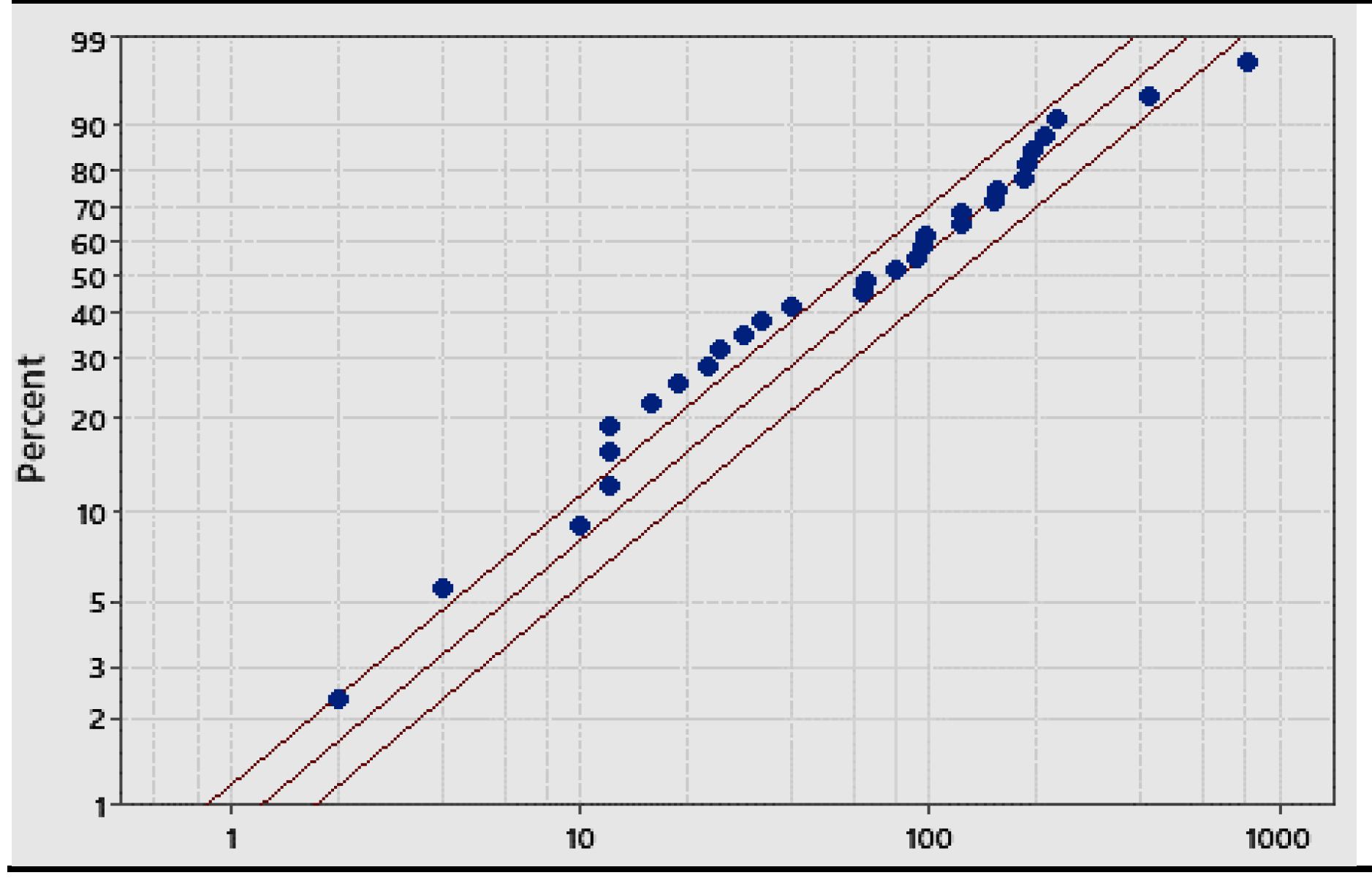
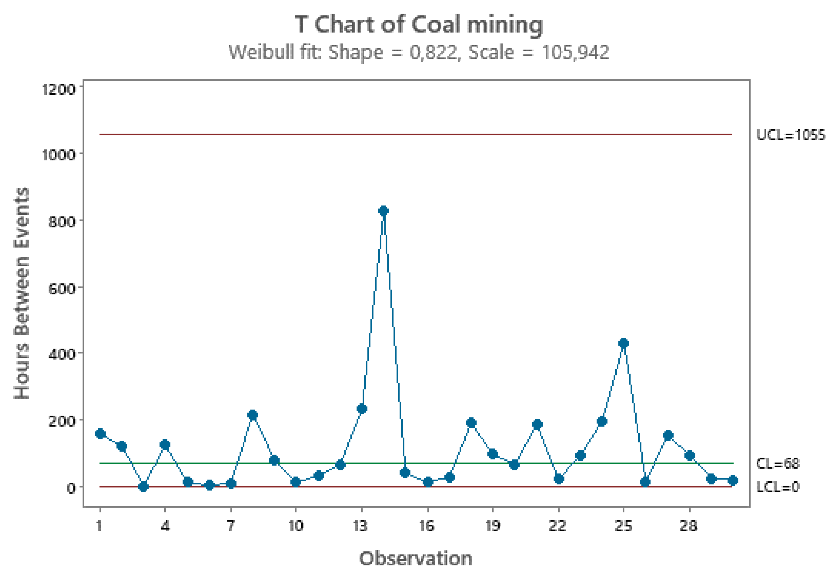
The analysis of the first 30 data show that three possible distributions can be considered, using Minitab 21: Weibull, Gamma, and Exponential; since the Weibull is acceptable, we could use it. See the Table 2.
Excerpt 9.
Formulae for the Control Limits for the first 30 data, IIE Transactions, (Zhang et al., 2006).
Excerpt 9.
Formulae for the Control Limits for the first 30 data, IIE Transactions, (Zhang et al., 2006).
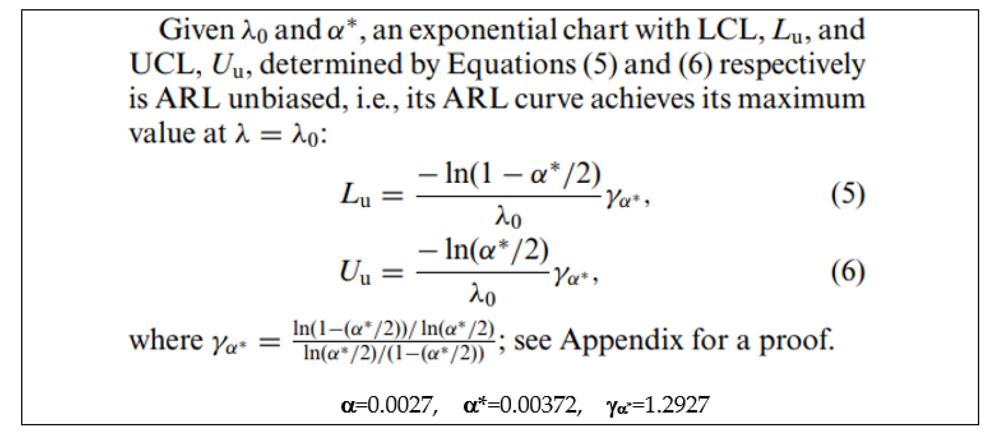
Figure 6.
The CC of the first m=30 observations used to find the Control Limits (logarithmic scale; only LCL shown). RIT used (exponential distribution, in spite of Table 2…): only LCL is shown because UCL1000.
Figure 6.
The CC of the first m=30 observations used to find the Control Limits (logarithmic scale; only LCL shown). RIT used (exponential distribution, in spite of Table 2…): only LCL is shown because UCL1000.
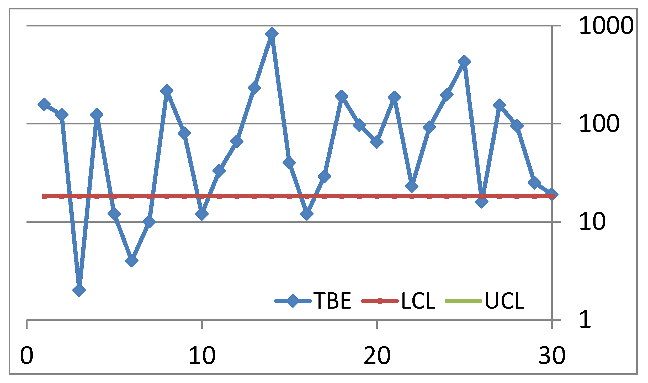
Anyway, for comparison with Zhang et al., 2006, we use the exponential distribution, which is not the “best” to be considered: as you can see the Process is OOC, with 7 points below the LCL.
Therefore, these data should be discarded for the computation of λ0.
Hence, the Control Limits (Zhang et al., 2006), based on the estimate “assumed as true” λ0=0.0081
| Lu=0.286 and LCLZhang=0.268 | Uu=966.6 and UCLZhang=1013.9 |
cannot be used for the next 160 data.
Is the statement (assumption!) “… first m=30 observations to be from the in-control process…” sound? NO! The Figure 9 proves [formulae (13)] that the process is OOC.
Using the formulae in the Excerpt 9, those authors do not extract the maximum information from the data in the Process Control.
Table 2.
Estimation of the possible distributions for the first m=30 observations.
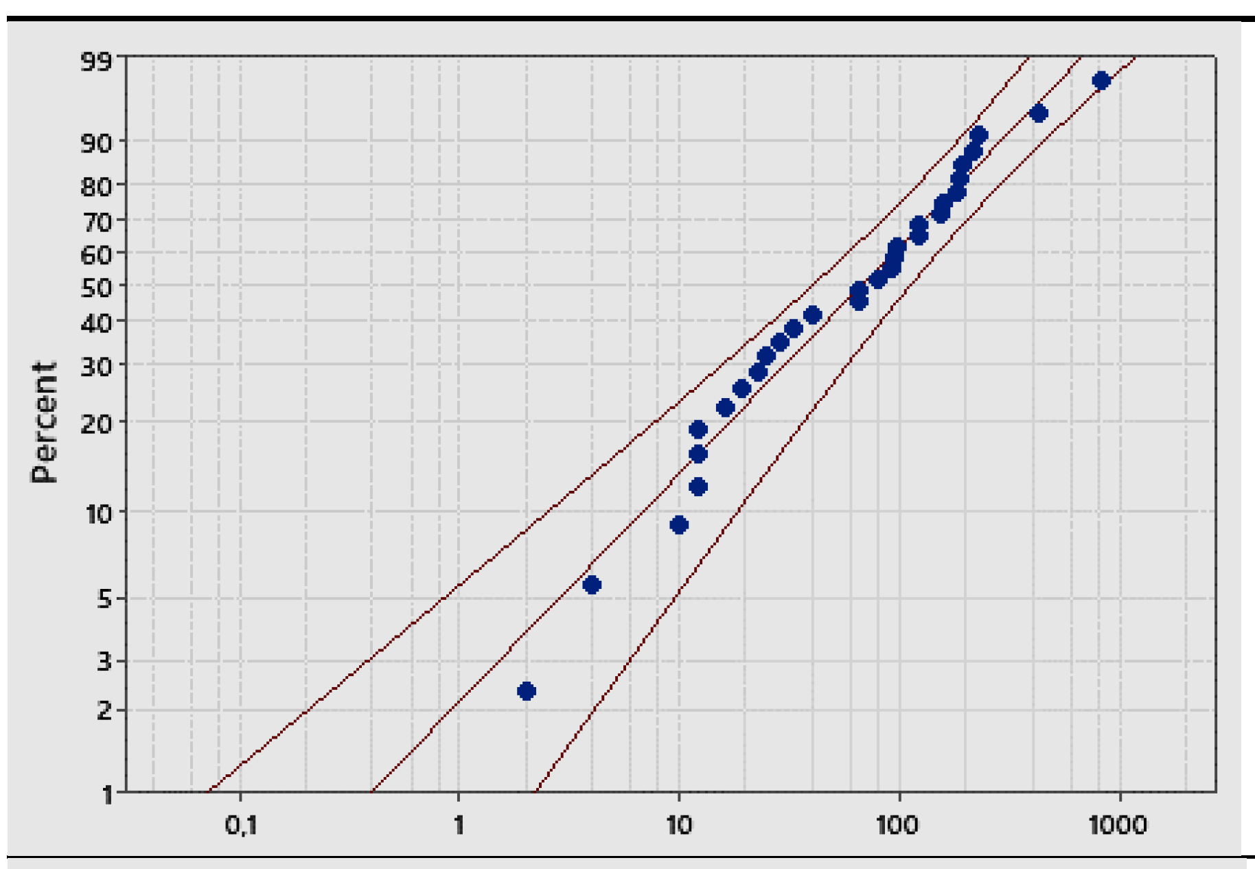 |
Weibull (95%)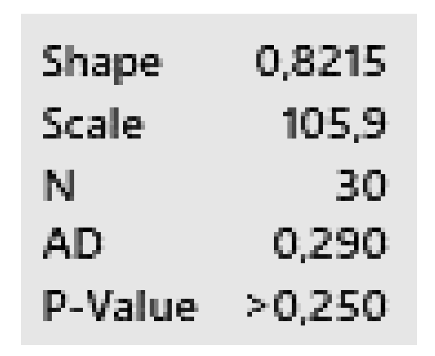 Scale: 105.94; Shape: 0.82 Scale: 105.94; Shape: 0.82 |
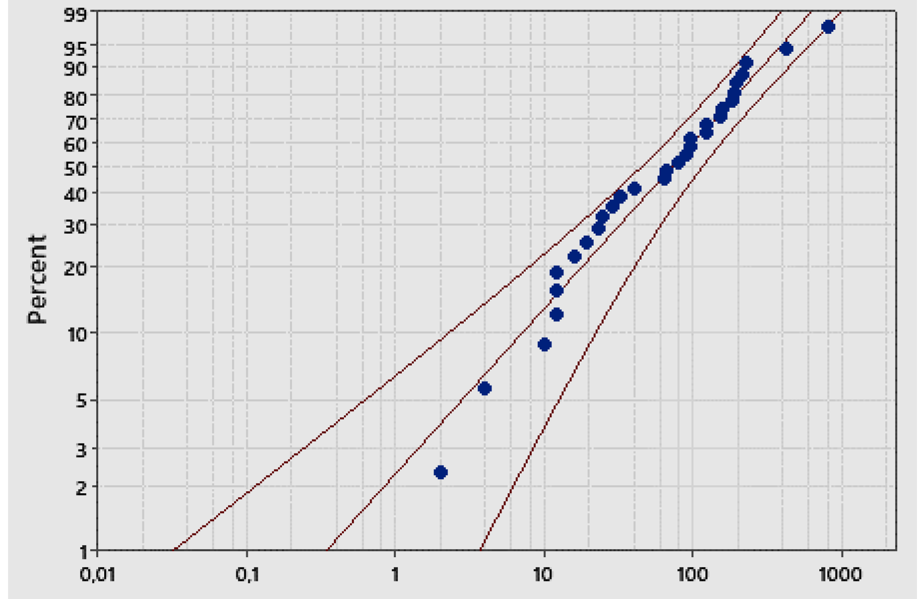 |
Gamma (95%)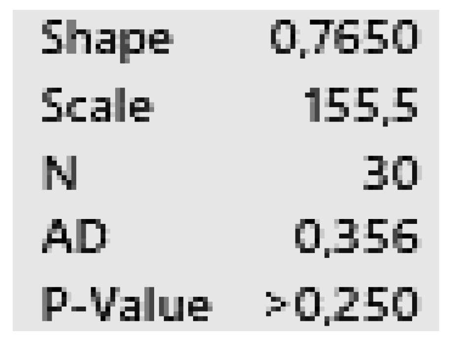 Scale: 155.47; Shape: 0.77 Scale: 155.47; Shape: 0.77 |
 |
Exponential (95%) Scale: 118.93, Shape: 1 Scale: 118.93, Shape: 1 |
Before ending this section, let’s see what MINITAB, which use the ideas of Santiago & Smith, provides us in Phase I (Figure 7a)
Figure 7a.
MINITAB CC of the first m=30 observations used to find the Control Limits (Minitab uses the formulae in the Appendix C, applied to Weibull distribution); process IC due to wrong Control Limits.
Figure 7a.
MINITAB CC of the first m=30 observations used to find the Control Limits (Minitab uses the formulae in the Appendix C, applied to Weibull distribution); process IC due to wrong Control Limits.
Notice that JMP (using the ideas of Santiago & Smith), provides us in Phase I the same type of information (Figure 7b)
Figure 7b.
JMP CC of the first m=30 observations used to find the Control Limits (JMP uses the formulae in the Appendix C, applied to Weibull distribution); process IC due to wrong Control Limits.
Figure 7b.
JMP CC of the first m=30 observations used to find the Control Limits (JMP uses the formulae in the Appendix C, applied to Weibull distribution); process IC due to wrong Control Limits.
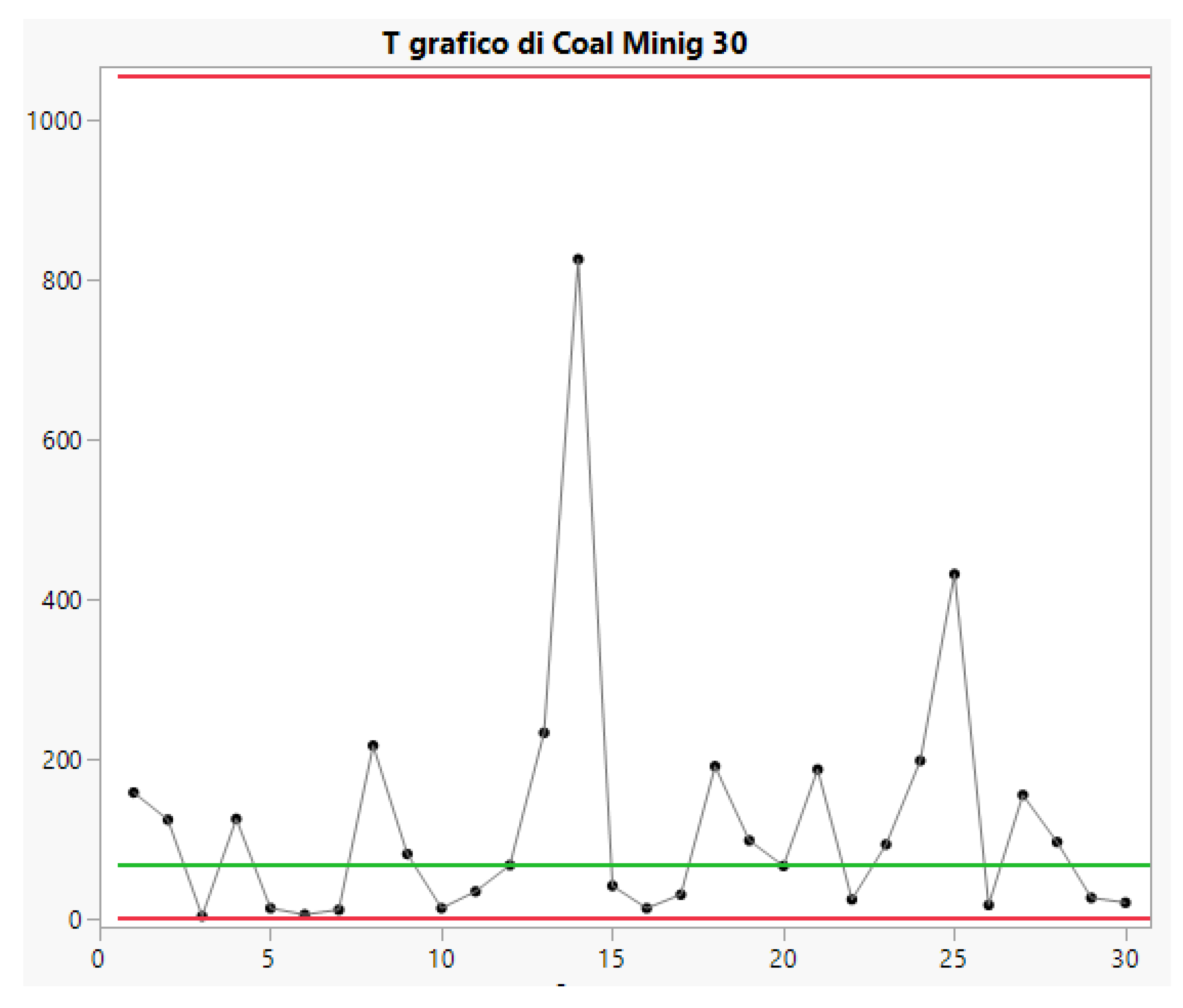
For the software Minitab, the process is IC, the same as Zhang et al. and Kumar et al.; same result could have been found by JMP (Appendix B) and SAS, and all the authors in the “Garden [24]”…
3.2. Control Charts for TBE Data. Phase II Analysis
We saw in the previous section what usually it is done during the Phase I of the application of CCs: estimation of the mean and standard deviation; later, their values are assumed as “true known” parameters of the data distribution, in view of the Phase II.
In particular, for TBE individual data the exponential distribution is assumed with a known parameter λ0 or θ0.
We consider now what it is done during the Phase II of the application of CCs for TBE data individual exponentially distributed.
We go on with the paper “Improved Shewhart-Type Charts for ….”, Journal of Quality Technology, 2016, (Kumar, Chakraborti et al. with various presence in the “Garden …”) who analysed the Jarret data. In their paper we read:
Excerpt 10.
From “Improved … Monitoring Times Between Events”, J. Quality Technology, ‘16.
They combining 4 data to generate a t4 chart giving the formulae in the Excerpt 10 (with r in place of 4; notice the authors mentioned… ).
Notice the formulae: the mentioned authors provide their LCL and UCL which are actually the Probability Limits L and U of the Probability Interval (PI) and NOT the Control Limits of the Control Chart, as it is easily seen By using the Theory of CIs (Figure 1 and Figure 5).
All the Jarret data [30+40 t4] are very interesting for our analysis; we recap the two important points, given by the authors (Chakraborti et al.):
- … first m=30 observations to be from the in-control process, from which we estimate … the mean TBE approximately, 123 days; we name it θ0.
- … we apply the t4-chart… Thus, … converted by accumulating a set of four consecutive failure times … the times until the fourth failure, used for monitoring the process to detect a change in the mean TBE.
The 3 authors (Chakraborti et al.) state: “… the control limits … t4-chart are seen to be equal to LCL=63.95, UCL=1669.28 with CL (Centre Line)=451.79”, named by them “ARL-unbiased {1/1, 1/1}”.
The 3 authors (Chakraborti et al.) state also: “… the control limits … t4-chart are seen to be equal to LCL=217.13, UCL=852.92 with CL (Centre Line)=451.79”, named by them “ARL-unbiased {M:3/4, M:3/4}”.
Dropping out the OOC data (from the first 30 observations), in Phase I, with RIT, we find that now the process is IC: the distribution fitting the remaining data is the Weibull with parameters η=140.6 days and β=1.39; since the CI of the shape parameter is 0.98-----2.15, with CL=90%, we can assume β=1 (exponential with θ=127.9); therefore, we have the “true” LCL=18.6, quite different from the LCLs of the authors (Chakraborti et al.).
Considering the 40 t4 data, the distribution fitting the data is the Weibull with parameters η=990.2 days and β=1.18; since the 1∈CI of the shape parameter, with CL=90%, we can assume β=1 (exponential with θ=924.5); therefore, we have the “true” LCL=72.9 and UCL=1987, quite different from the Control Limits of the authors (Kumar, Chakraborti et al.): hence there is a profound consequence on the analysis of the t4-chart; see the Figure 12.
Excerpt 11.
From “Improved … Monitoring Times Between Events”, J. Quality Technology, ‘16.
Considering, on the contrary, the value θ=127.9 from the first [<30] INDIVIDUAL observations of the IC process, transformed into the one for the t4 chart, we have the “true” LCL=40.38 and UCL=1100.37; so, we have 4 LCLs and 4 UCLs (see Figure 12).
The 3 authors (Kumar, Chakraborti et al.) show the formulae for the Control Limits (Excerpt 11):
Now we face a problem: in which way could the 3 authors (Kumar, Chakraborti et al.) compute their Control Limits from the individual first m=30 observations?
FG (in spite of Excerpt 11) did not find the way: is θ0=1/λ0 the value estimated from the first m=30 observations? He suspects that they used a trick (not shown): they use the fist 30 data to find θ0=123 days (from the total t0 of days in the Phase I) and then, they consider the total as though it were 4t0, i.e. 30 t4, to find LCL and UCL for the t4-chart … We did it, but we could not find them…
Doing that, Chakraborti et al. missed the fact that the process, in the individual first m=30 observations was OOC and they should not use the ″λ0 specified value of the failure rate, that has to be estimated from a preliminary IC sample.″
Since the data are assumed (by the 3 authors) Exponentially distributed it follows from the Theory that “… by accumulating a set of four consecutive failure times (times until the fourth failure)…” we should find the t4 data (determinations of the RV T4) Erlang distributed. Since k=4 we could expect that the CLT could apply and find that the 40 t4 data (determinations of the 40 RV T4) follow “approximately” the Normal distribution.
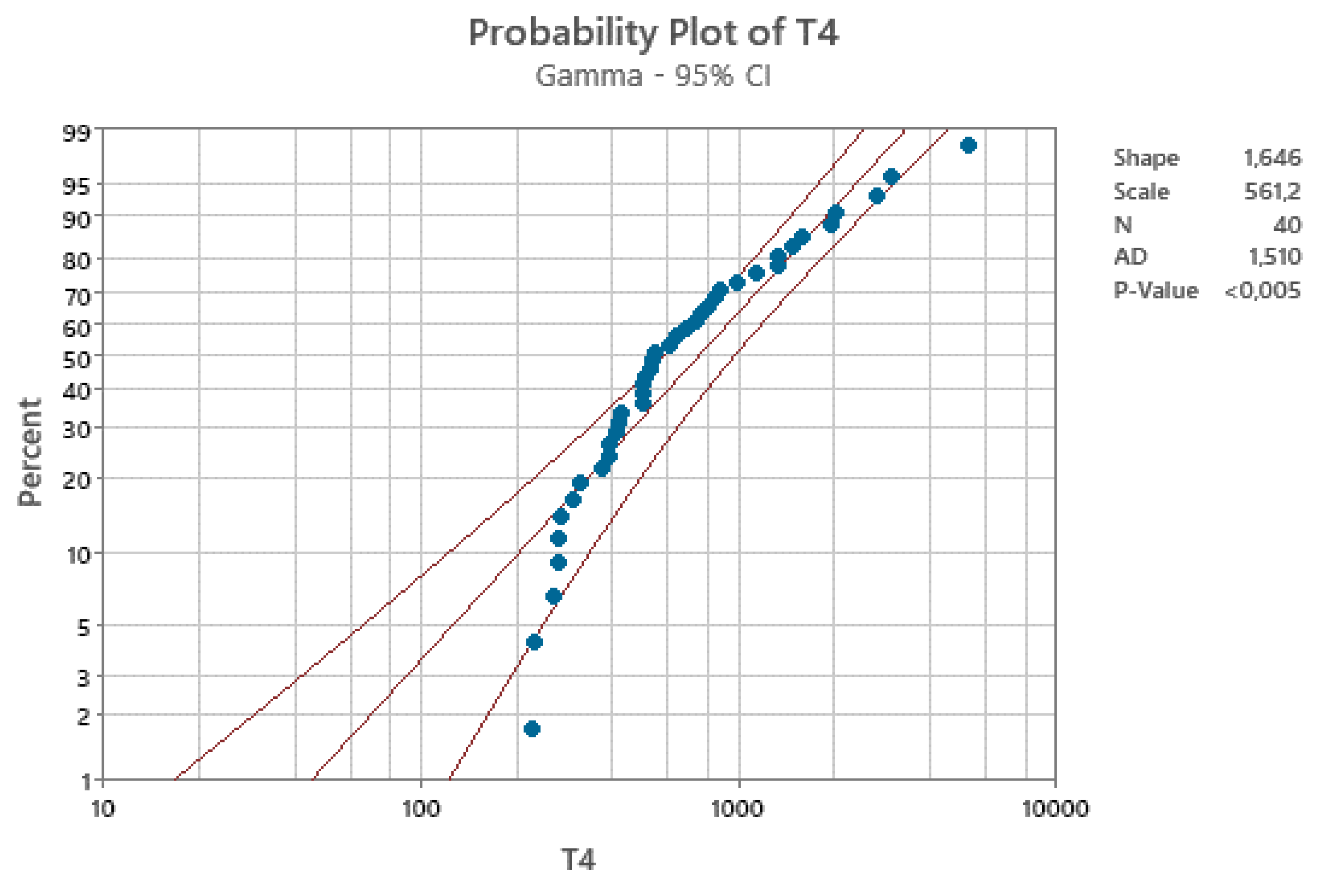
Considering the 40 t4 data and searching for the distribution, we are disillusioned: the distributions Normal, Lognormal, Exponential, Gamma, Smallest Extreme, Largest Extreme, Logistic, Loglogistic do not fit the data; only the Weibull, and the Box-Cox and Johnson transformations seem adequate… See the Gamma (Erlang) fitting in the Figure 8.
Figure 8.
Fitting of the Gamma distribution to the 40 t4 data: the Erlang expected distribution is not applicable to the 40 t4 data.
Figure 8.
Fitting of the Gamma distribution to the 40 t4 data: the Erlang expected distribution is not applicable to the 40 t4 data.
Therefore, the authors formulae for the Control Limits are inadequate in three ways, because
- a)
- the gamma (Erlang) distribution does not apply, with CL=95%
- b)
- then, the formulae in the Excerpt 11 cannot be applied.
- c)
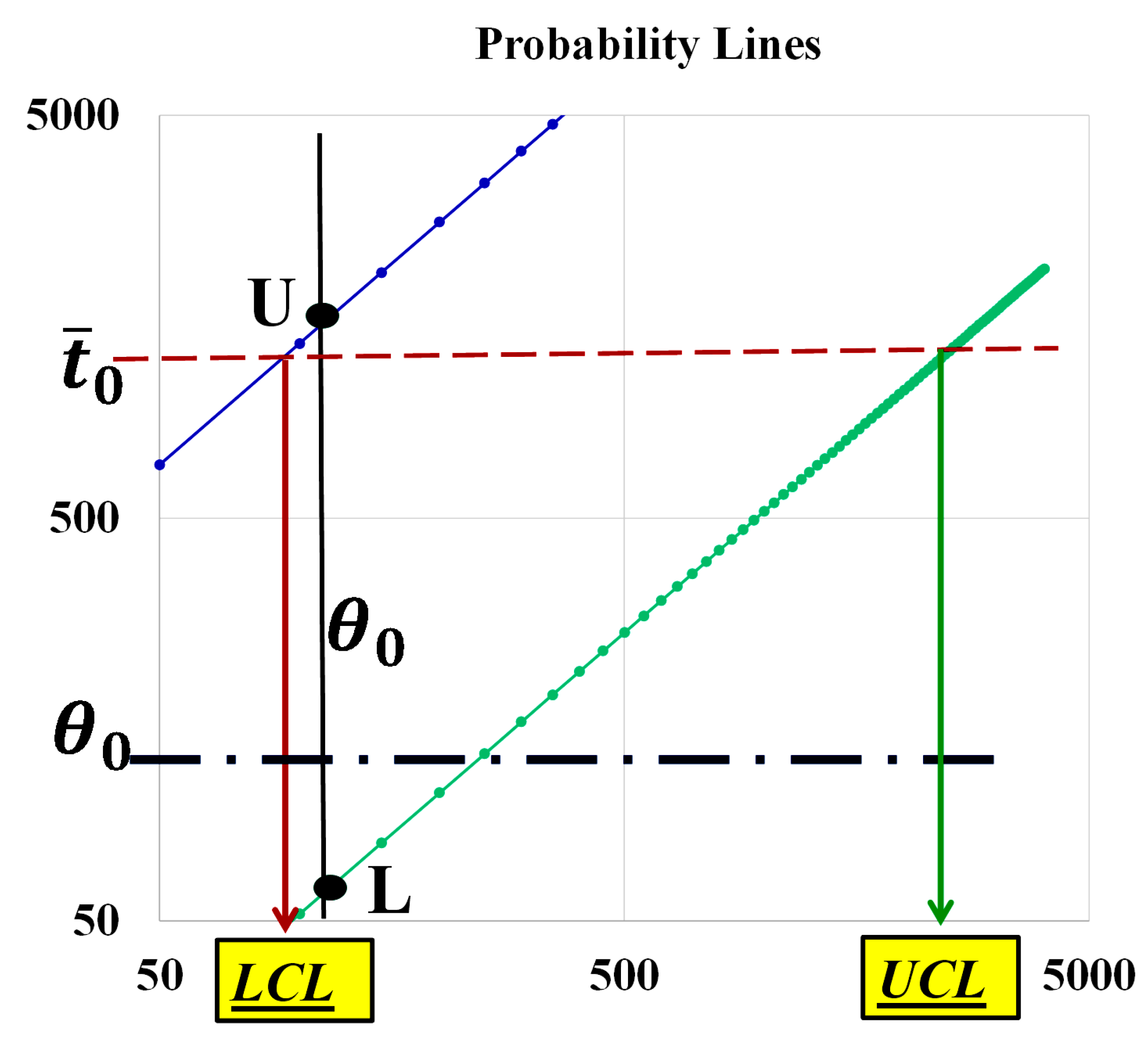
- the formulae, in their paper, and are generated by the confusion (of the authors) between LCL and L and UCL and U, as you can see in the Figure 9, based on the non-applicable Gamma distribution; you see the vertical line intercepting the two probability lines in the points L and U such that and versus the horizontal line, at intercepting the two lines at LCL and UCL.
It is clear that the two intervals, L-----U and LCL-----UCL, are different and have different definitions, meaning and length, through the Theory [6,7,8,11,12,13,14,15,16,25,26,27,28,29,30,31,32,33,34,35,36]. Notice, in the Figure 9, the logarithmic scale for both axes (to have readable intervals).
It should be noted that we drew two horizontal lines, one at (the experimental mean) and the other at (the assumed known mean) to show the BIG difference between the interception points: we showed the TRUE LCL and UCL; the reader can guess that the WRONG Control Limits (not shown in the figure) have quite different values from the TRUE Control Limits.
Figure 9.
The two intervals L-----U and LCL-----UCL are different (different definitions and meaning). Axes logarithmic (to have readable intervals). Notice the two horizontal lines at and at ….
Figure 9.
The two intervals L-----U and LCL-----UCL are different (different definitions and meaning). Axes logarithmic (to have readable intervals). Notice the two horizontal lines at and at ….
The reader is humbly asked to be very attentive in the analysis of the Figure 9: FG thanks him!
Using the original 160 data, divided in 40 samples of size 4, we could compare the estimates with those found by the 40 t4 (in the paper “Improved … for Monitoring TBE”, Journal of Quality Technology, 2016”); you see them in the Table 3.
Notice that the Figure 10a shows the same behaviour as the Phase I figure; it would be interesting to understand IF, with that, the authors would have been able to find an ARL=370: the process is Out Of Control both considering the first individual 30 data and the last individual 160 data ….
How many OOC are in the Jarret data?
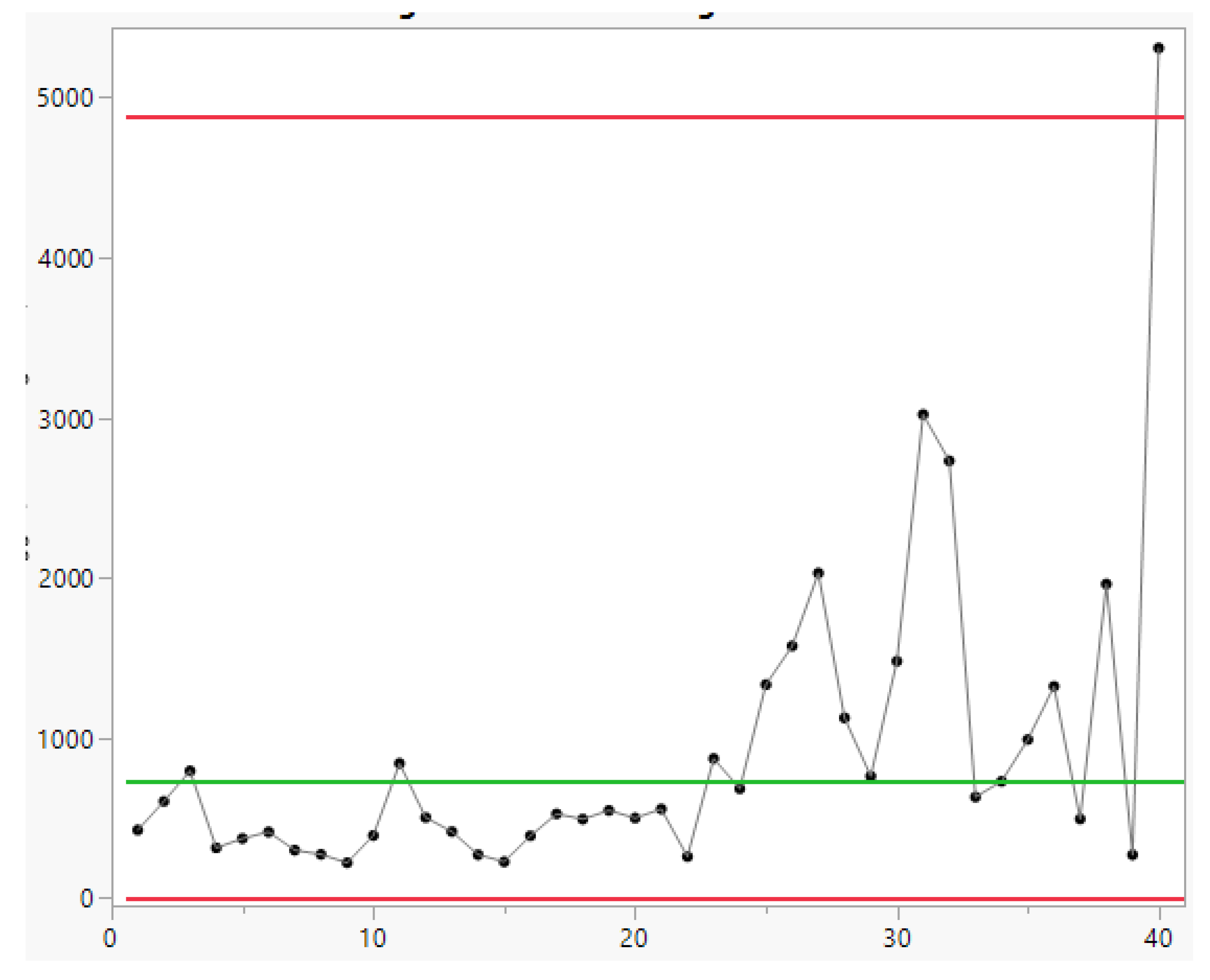
Analysing the 40 t4 data with Minitab (which uses the Santiago&Smith formulae, Appendix C) we get Figure 11a, and with JMP we get Figure 11b;
Figure 10a.
Control Charts and LCL from the last 160 data. Process OOC: 35 points below the LCL. Vertical axis logarithmic. RIT used.
Figure 10a.
Control Charts and LCL from the last 160 data. Process OOC: 35 points below the LCL. Vertical axis logarithmic. RIT used.
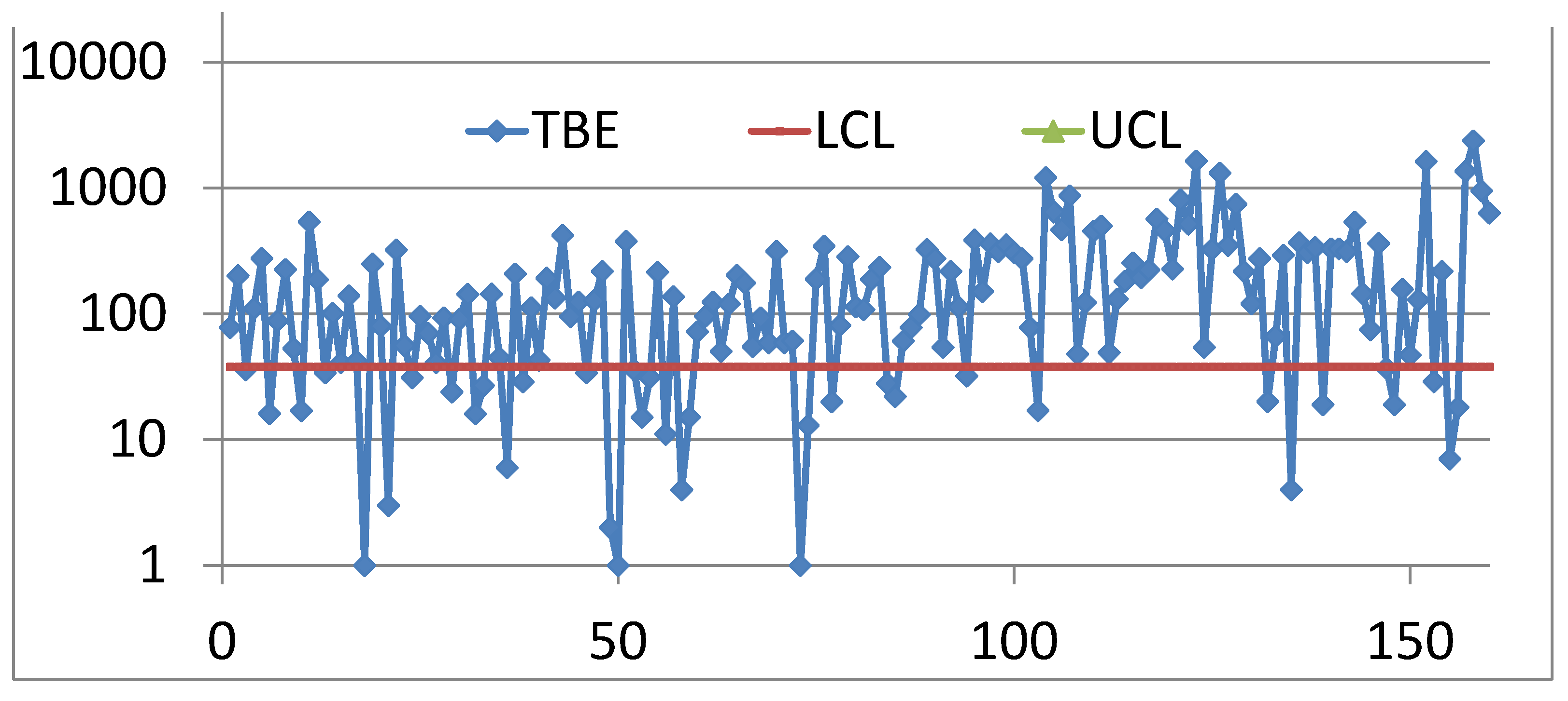
Figure 10b.
T Chart computed by JMP for the last 160 data. Process IC: opposite to Figure 10 a.
Figure 10b.
T Chart computed by JMP for the last 160 data. Process IC: opposite to Figure 10 a.
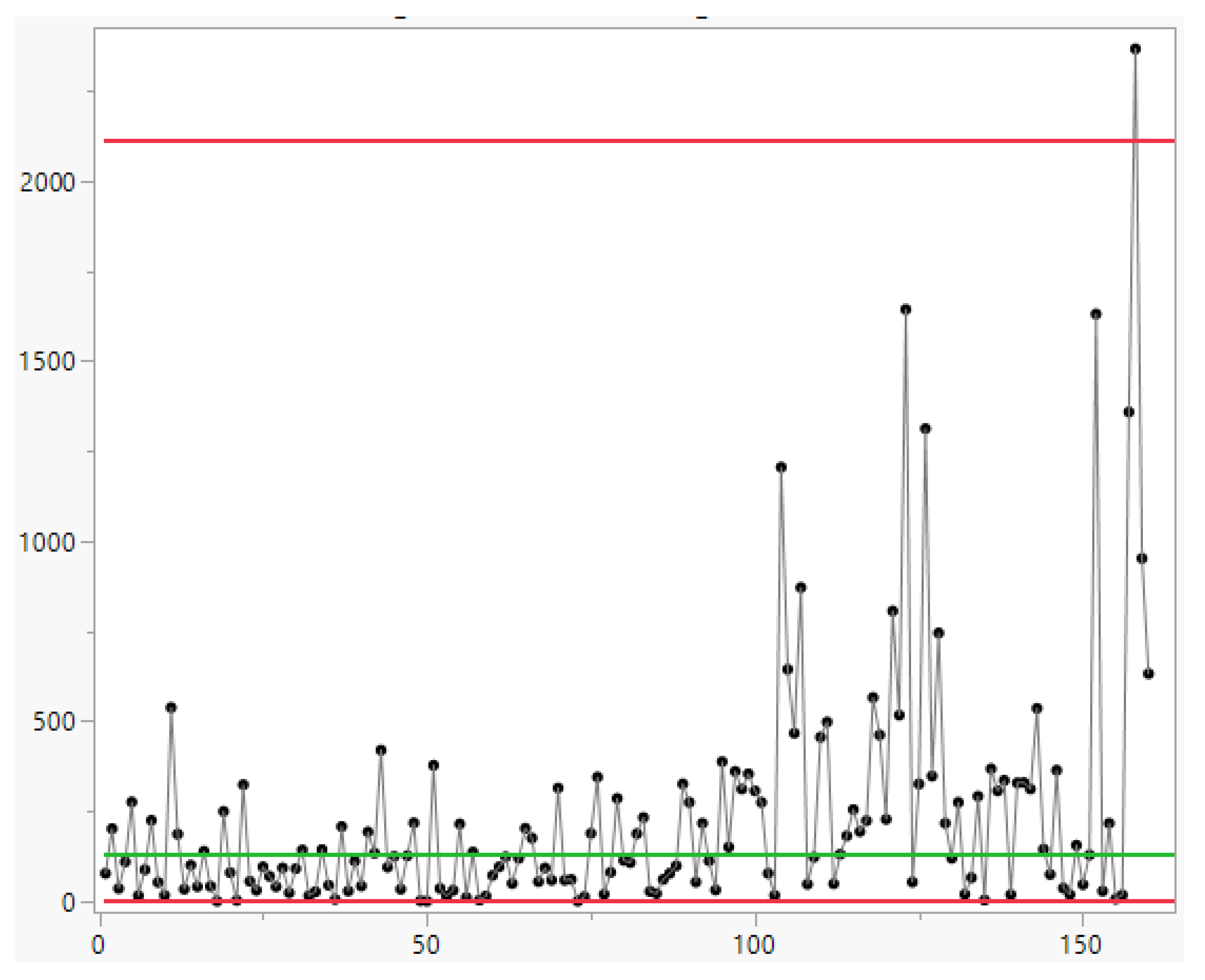
Figure 11a.
T Chart for the 40 t4 data. Minitab T-Chart (by Santiago & Smith).
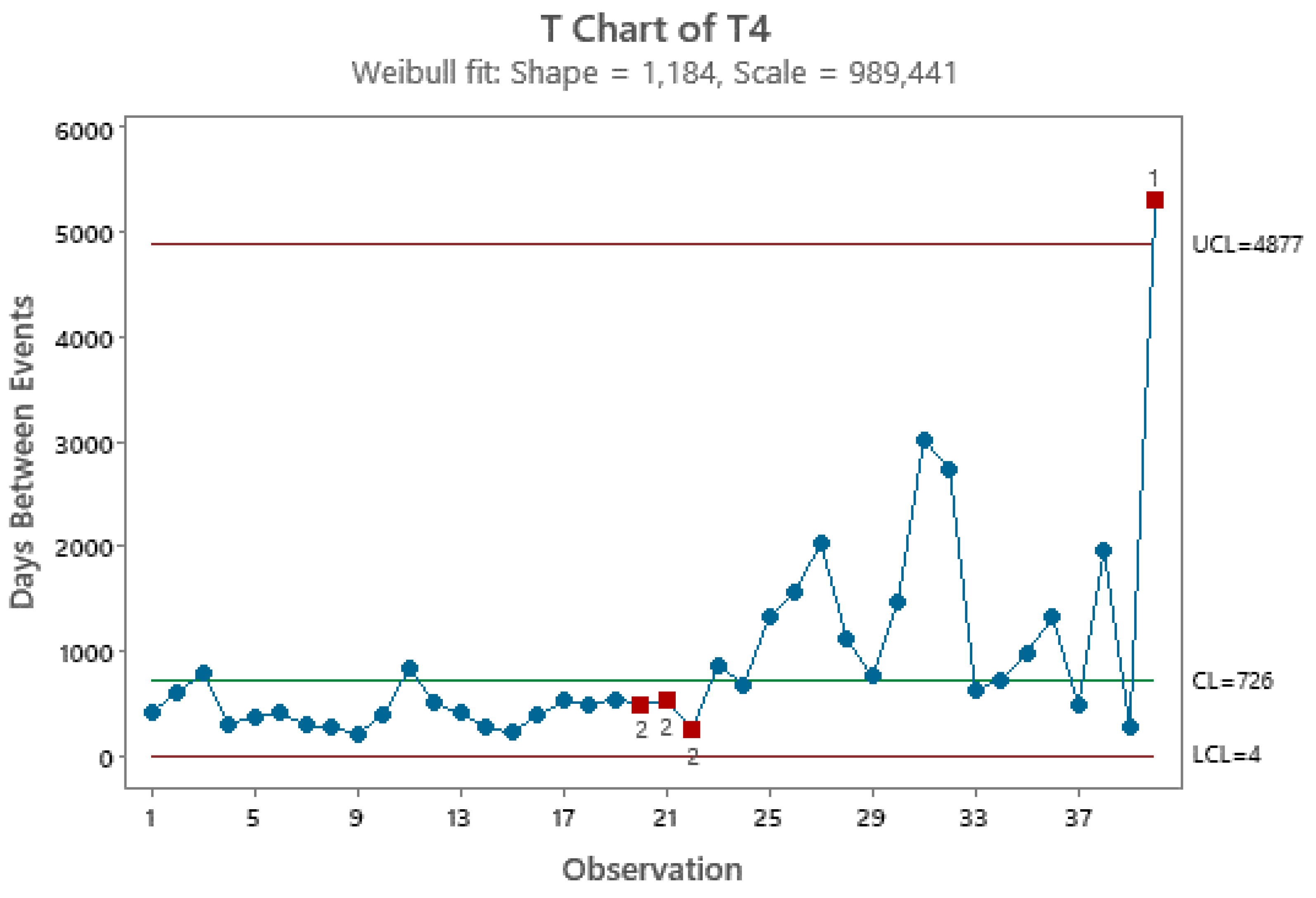
Figure 11b.
T Chart for the 40 t4 data, computed with JMP; compare with Figure 11a.
Figure 11b.
T Chart for the 40 t4 data, computed with JMP; compare with Figure 11a.
See the authors Acknowledgement (in the paper)….
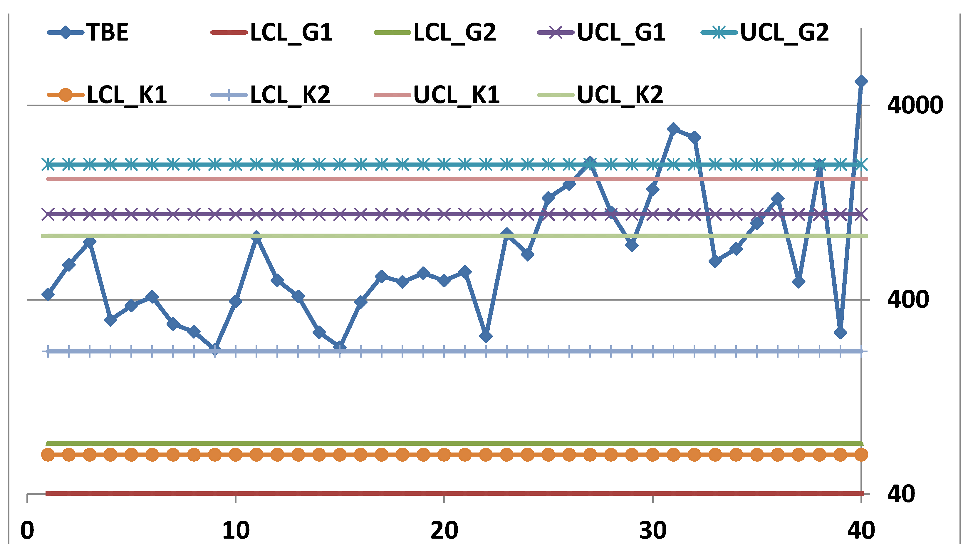
Notice that the OOC points in the Figure 10 disappear when we plot the 40 t4, as you can see in the Figure 12, where we draw 4 LCLs and 4 UCLs, from Kumar, Chakraborti et al. analysis and FG analysis (with RIT). We have the Figure 12.
| LCL_K1 | LCL_K2 | UCL_K1 | UCL_K2 | LCL_G1 | LCL_G2 | UCL_G1 | UCL_G2 |
| 63.95 | 217.13 | 1669.28 | 852.92 | 40.38 | 72.91 | 1100.37 | 1986.96 |
Figure 12.
Control Charts and LCL from the 40 t4, data. Notice: we draw 4 LCLs and 4 UCLs.
That the Method is fundamental to draw sound decisions.
Which is the best Method? Only the one which is Scientific, based on a sound Theory. Which one?
From the Theory [6,7,8,11,12,13,14,15,16,25,26,27,28,29,30,31,32,33,34,35,36] we know that we must assess the “true (to be used in the Phase II)” Control Limits from the data of an IC Process in the Phase I: therefore, only LCL_G1=40.38 and UCL_G1=1100.37 are the Scientific Control Limits; you can compare with the others in Figure 12.
From Figure 12 we see that the first 20 t4 have a mean lower than the last 20 t4: the mean time between events increased with calendar time. We can assess that by computing the two mean values: their ratio is 3.18 and we can see if it is significant and we find that it is so with CL=0.9973 (0.0027 probability of being wrong).
See also Figure 13a,b.
Figure 13.
(a) First 20 t4 data. (b) Second 20 t4 data.
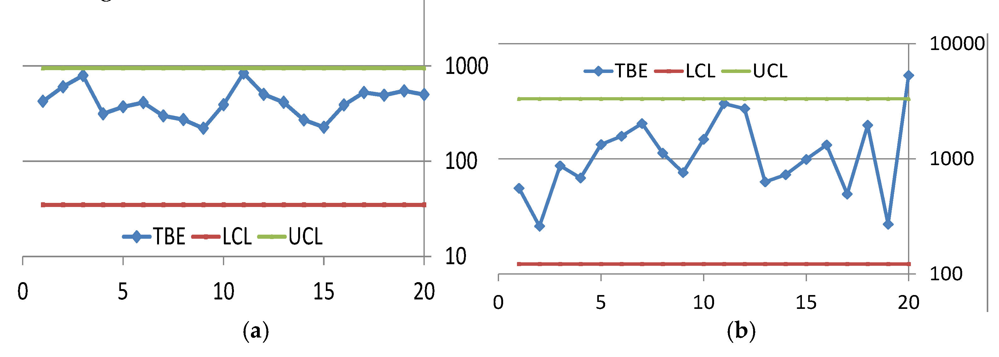
From Figure 11a,b, Figure 12 and Figure 13ab we saw that the mean time between explosions was changing with time: it became larger (improved); a method that should show better this behaviour is the EWMA Control Chart. We do not analyse this point; also, for this chart there is the problem of the confusion between the intervals L-------U and LCL-------UCL.
4. Discussion
We first considered the c Chart (paper [3]) and saw that a method exists for better computation of LCL-------UCL. Later, we decided to use the Jarrett (1979) data in Table 1 and the analysis by Kumar, Chakraborti, Rakitzis, (2017) in the Journal of Quality Technology [4] and that by Zhang, Xie, Goh (2006) in the IIE Transactions [5], (papers that you can find also in the “Garden of flowers” [24] and in the Appendix C).
We got different results from all those authors: the cause is that they use the Probability Limits of the PI (Probability Interval) as they were the Control Limits (so named by them) of the Control Charts.
The proof of the confusion between the intervals L-------U (Probability Interval) and LCL-------UCL (Confidence Interval) in the domain of Control Charts (for Process Management) highlight the importance and novelty of these ideas in the Statistical Theory and in the applications.
For the “location” parameter in the CCs, from the Theory, we know that two mean (parameter), q=1,2, …, n, and any other mean (parameter), r=1,2, …, n, are different, with risk α, if their estimates are not both included in their common Confidence Interval as the CI of the grand mean (parameter) is.
Let’s consider the formula (4) and apply it to a “Normal model” (due to CLT, and assuming known variance), sequentially we can write the “real” fixed interval L----U comprising the RV (vertical interval) and the Random Interval comprising the unknown mean (horizontal interval) (Figure 14)
When the RV assume its determination (numerical value) (grand mean) the Random Interval becomes the Confidence Interval for the parameter μ, with CL=1-α: risk α that the horizontal line does not comprise the “mean” μ.
This is particularly important for the Individual Control Charts for Exponential, Weibull and Gamma distributed data: this is what Deming calls “Profound Knowledge (understanding variation)” [9,10]. In this case, the Figure 14 looks like the Figure 1, where you see the Confidence Interval, the realisation of the horizontal Random Interval.
The case we considered shows clearly that the analyses, in the Process Management, taken so far have been wrong and the decisions have been misleading, when the collected data follow a Non-Normal distribution [24].
Since a lot of papers (related to Exponential, Weibull and Gamma distributions), with the same problem as that of “The garden of flowers” [24], are published in reputed Journals we think that the title “History is written by the winners. Reflections on Control Charts for Process Control” is suitable for this paper: the authors of the wrong papers [24] are the winners.
Our study is limited to the Individual Control Charts with Exponentially, Weibull and Gamma distributed data.
Further studies should consider other distributions which cannot be transformed into the three above distributions: Exponential, Weibull and Gamma.
5. Conclusions
With our figures (and the Appendix C, that is a short extract from the “Garden … [24]”) we humbly ask the readers to look at the references [1,2,3,4,5,6,7,8,9,10,11,12,13,14,15,16,17,18,19,20,21,22,23,24,25,26,27,28,29,30,31,32,33,34,35,36,37,38,39,40,41,42,43,44,45,46] and find how much the author has been fond of Quality and Scientificness in the Quality (Statistics, Mathematics, Thermodynamics, …) Fields.
The errors, in the “Garden … [24]”, are caused by the lack of knowledge of sound statistical concepts about the properties of the parameters of the parent distribution generating the data, and the related Confidence Intervals. For the I-CC_TBE the computed Control Limits (which are actually the Confidence Intervals), in the literature are wrong due to lack of knowledge of the difference between Probability Intervals (PI) and Confidence Intervals (CI); see the Figure 17 (remembering also the Figure 1 and Figure 14). Therefore, the consequent decisions about Process IC and OOC are wrong.
We saw that RIT is able to solve various problems in the estimation (and Confidence Interval evaluation) of the parameters of distributions for Control Charts. The basics of RIT have been given.
We could have shown many other cases (from papers not mentioned here, that you can find in [22,23,24]) where errors were present due to the lack of knowledge of RIT and sound statistical ideas.
Following the scientific ideas of Galileo Galilei, the author many times tried to compel several scholars to be scientific (Galetto 1981-2025). Only Juran appreciated the author’s ideas when he mentioned the paper “Quality of methods for quality is important” at the plenary session of EOQC Conference, Vienna. [1]
For the control charts, it came out that RIT proved that the T Charts, for rare events and TBE (Time Between Events), used in the software Minitab, SixPack, JMP or SAS are wrong. So doing the author increased the h-index of the mentioned authors who published wrong papers.
RIT allows the scholars (managers, students, professors) to find sound methods also for the ideas shown by Wheeler in Quality Digest documents.
We informed the authors and the Journals who published wrong papers by writing various letters to the Editors…: no “Corrective Action”, a basic activity for Quality has been carried out by them so far. The same happened for Minitab Management. We attended a JMP forum in the JMP User Community and informed them that their “Control Charts for Rare Events” were wrong: they preferred to stop the discussion, instead to acknowledge the JMP faults [46].
So, dis-quality continues to be diffused people and people continue taking wrong decisions…
Deficiencies in products and methods generate huge cost of Dis-quality (poor quality) as highlighted by Deming and Juran. Any book and paper are products (providing methods): their wrong ideas and methods generate huge cost for the Companies using them. The methods given here provide the way to avoid such costs, especially when RIT gives the right way to deal with Preventive Maintenance (risks and costs), Spare Parts Management (cost of unavailability of systems and production losses), Inventory Management, cost of wrong analyses and decisions.
We think that we provided the readers with the belief that Quality of Methods for Quality is important.
The reader should remember the Deming’s statements and the ideas in [6,7,8,9,10,11,12,13,14,15,16,17,18,19,20,21,22,23,24,25,26,27,28,29,30,31,32,33,34,35,36,37,38,39,40,41,42,43,44,45,46].
Unfortunately, many authors do not know Scientifically the role (concept) of Confidence Intervals (Appendix B) for Hypothesis Testing.
Therefore, they do not extract the maximum information form the data in the Process Control.
Control Charts are a means to test the hypothesis about the process states, H0={Process In Control} versus H1={Process Out Of Control}, with stated risk α=0.0027.
We have a big problem about Knowledge: sound Education is needed.
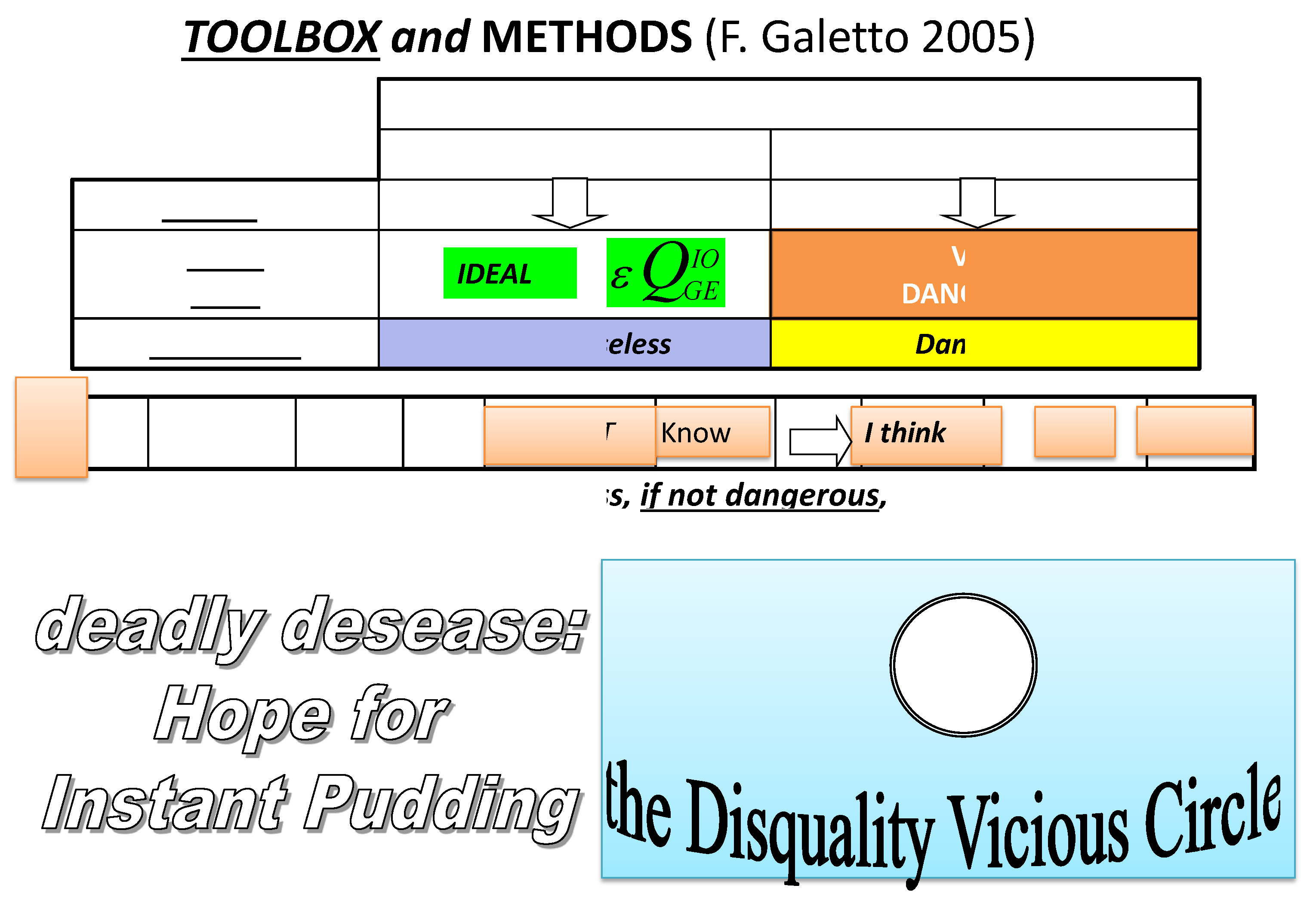
We think that the Figure 16 conveys the fundamental ideas about the need of Theory for devising sound Methods, to be used in real applications in order to avoid the Dis-quality Vicious Circle.
Humbly, given our commitment to Quality, Education, Mathematics anf Physics (versus wrong methods: Fuzzy, Taguchi, Six-Sigma, Control Charts, …) and our long-life love for them [1,2,3,4,5,6,7,8,9,10,11,12,13,14,15,16,17,18,19,20,21,22,23,24,25,26,27,28,29,30,31,32,33,34,35,36,37,38,39,40,41,42,43,44,45,46], we would venture to quote Voltaire:
“It is dangerous to be right in matters on which the established men are wrong.” because “Many are destined to reason wrongly; others, not to reason at all; and others, to persecute those who do reason.” So, “The more often a stupidity is repeated, the more it gets the appearance of wisdom.” and “It is difficult to free fools from the chains they revere.”
Let’s hope that Logic and Truth prevail and allow our message to be understood (Figure 15 and Figure 16).
Figure 15.
Probability Intervals L-----U versus Confidence Intervals LCL-----UCL in Control Charts.
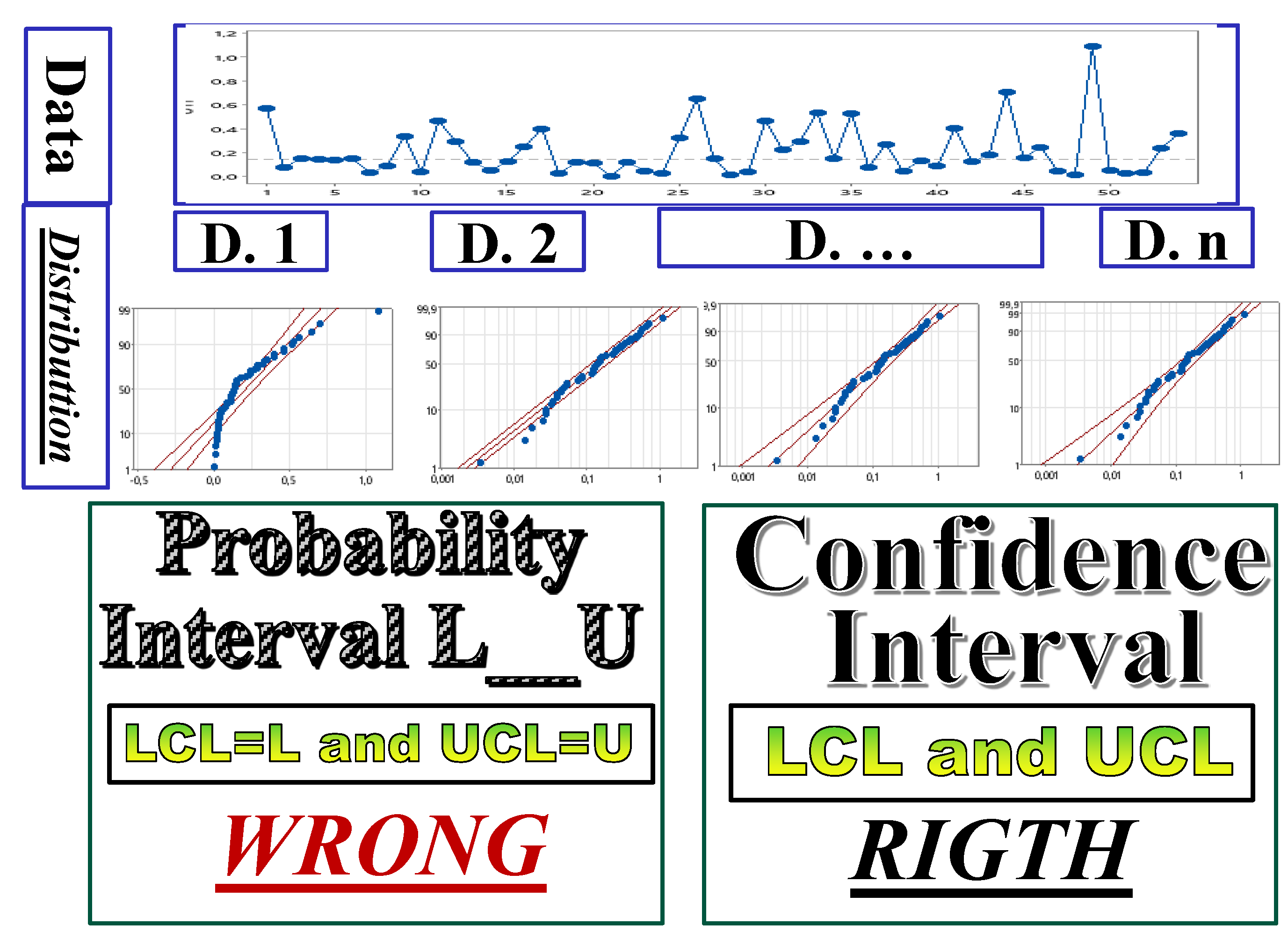
Figure 16.
Knowledge versus Ignorance, in Tools and Methods.
The objective of collecting and analysing data is to take the right action. The computations are merely a means to characterize the process behaviour. However, it is important to use the right Control Limits take the right action about the process states, i.e., In Control versus Out Of Control.
On July-August 2024 we again verified (through Six????? new downloaded papers) that the Pandemic Disease about the (wrong) Control Limits, that are actually the Probability Limits of the PI is still present (notice the Journals):
- Zameer Abbas et al., (30 June 2024): “Efficient and distribution-free charts for monitoring the process location for individual observations”, Journal of Statistical Computation and Simulation,
- Marcus B. Perry (June 2024) [University of Alabama 674 Citations] “Joint monitoring of location and scale for modern univariate processes”, Journal of Quality Technology.
- E. Afuecheta et al., (2023) “A compound exponential distribution with application to control charts”, Journal of Computational and Applied Mathematics [the authors use data of Santiago&Smith (Appendix C) and erroneously find that the UTI process IC].
- N. Kumar (2019), “Conditional analysis of Phase II exponential chart for monitoring times to an event”, Quality Technology & Quantitative Management
- N. Kumar (2021), “Statistical design of phase II exponential chart with estimated parameters under the unconditional and conditional perspectives using exact distribution of median run length”, Quality Technology & Quantitative Management
- S. Chakraborti et al. (2021), “Phase II exponential charts for monitoring time between events data: performance analysis using exact conditional average time to signal distribution”, Journal of Statistical Computation and Simulation
- S. Chakraborti et al. (2025), “Dynamic Risk-Adjusted Monitoring of Time Between Events: Applications of NHPP in Pipeline Accident Surveillance”, downloaded from RG
Other papers with the same problem have been downloaded from June 2024 to October 2025…
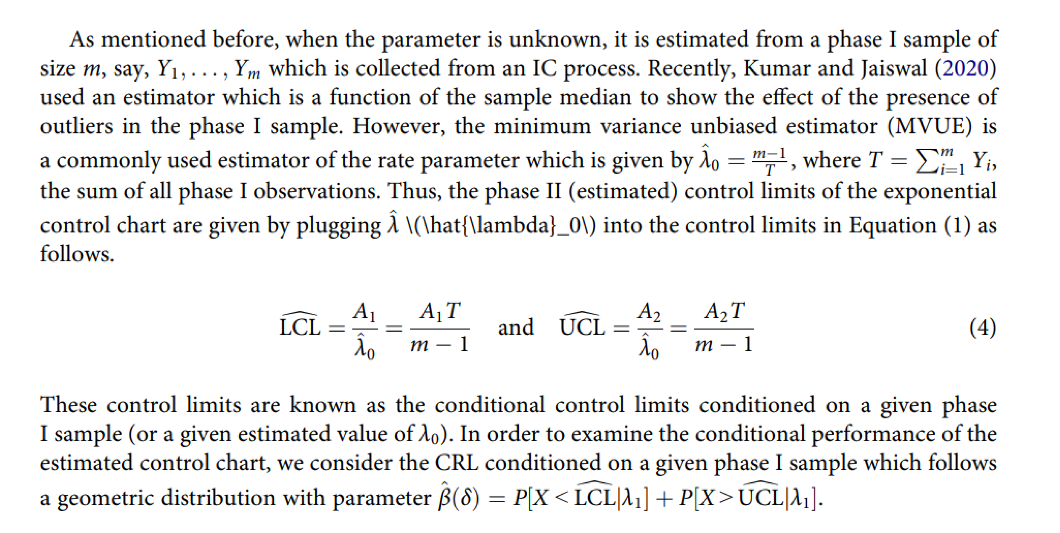
There will be any chance that the Pandemic Disease ends? See the Excerpt 12: notice the (ignorant) words “plugging into …”. The only way out is Knowledge… (Figure 16): Deming’s [7,8] Profound Knowledge, Metanoia, Theory.
Excerpt 12.
From “Conditional analysis of Phase II exponential chart… an event”, Q. Tech. & Quantitative Mgt, ’19.
Excerpt 12.
From “Conditional analysis of Phase II exponential chart… an event”, Q. Tech. & Quantitative Mgt, ’19.
Funding
This research received no external funding.
Data Availability Statement
“MDPI Research Data Policies” at https://www.mdpi.com/ethics.
Acknowledgments
In this section, you can acknowledge any support given which is not covered by the author contribution or funding sections. This may include administrative and technical support, or donations in kind (e.g., materials used for experiments).
Conflicts of Interest
“The author declares no conflicts of interest.”
Abbreviations
The following abbreviations are used in this manuscript:
| LCL, UCL | Control Limits of the Control Charts (CCs) |
| L, U | Probability Limits related to a probability 1-α |
| θ | Parameter of the Exponential Distribution |
| θL-----θU | Confidence Interval of the parameter θ |
| RIT | Reliability Integral Theory |
Appendix A
A Very Illuminating Case
We consider a case found in the paper (with 148 mentions) “Control Charts based on the Exponential distribution”, Quality Engineering, March 2013, of Santiago&Smith, two experts of Minitab Inc. at that time. You find it mentioned in the “Garden…” [24] and in the Appendix C.
This is important because we analysed the data with Minitab software and JMP software and we found astonishing results: the cause are the formulae .
The author knew that Minitab computes wrongly the Control Limits of the Individual Control Chart. He wanted to assess how the JMP Student Version would deal with them using the following 54 data analysed by Santiago&Smith in their paper; they are “Urinary Tract Infection (UTI) data collected in a hospital”; the distribution of the data is the Exponential.
Table A1.
UTI data (“Control Charts based on the Exponential distribution”).
| UTI | UTI | UTI | UTI | UTI | UTI | ||||||
| 1 | 0.46014 | 11 | 0.46530 | 21 | 0.00347 | 31 | 0.22222 | 41 | 0.40347 | 51 | 0.02778 |
| 2 | 0.07431 | 12 | 0.29514 | 22 | 0.12014 | 32 | 0.29514 | 42 | 0.12639 | 52 | 0.03472 |
| 3 | 0.15278 | 13 | 0.11944 | 23 | 0.04861 | 33 | 0.53472 | 43 | 0.18403 | 53 | 0.23611 |
| 4 | 0.14583 | 14 | 0.05208 | 24 | 0.02778 | 34 | 0.15139 | 44 | 0.70833 | 54 | 0.35972 |
| 5 | 0.13889 | 15 | 0.12500 | 25 | 0.32639 | 35 | 0.52569 | 45 | 0.15625 | ||
| 6 | 0.14931 | 16 | 0.25000 | 26 | 0.64931 | 36 | 0.07986 | 46 | 0.24653 | ||
| 7 | 0.03333 | 17 | 0.40069 | 27 | 0.14931 | 37 | 0.27083 | 47 | 0.04514 | ||
| 8 | 0.08681 | 18 | 0.02500 | 28 | 0.01389 | 38 | 0.04514 | 48 | 0.01736 | ||
| 9 | 0.33681 | 19 | 0.12014 | 29 | 0.03819 | 39 | 0.13542 | 49 | 1.08889 | ||
| 10 | 0.03819 | 20 | 0.11458 | 30 | 0.46806 | 40 | 0.08681 | 50 | 0.05208 |
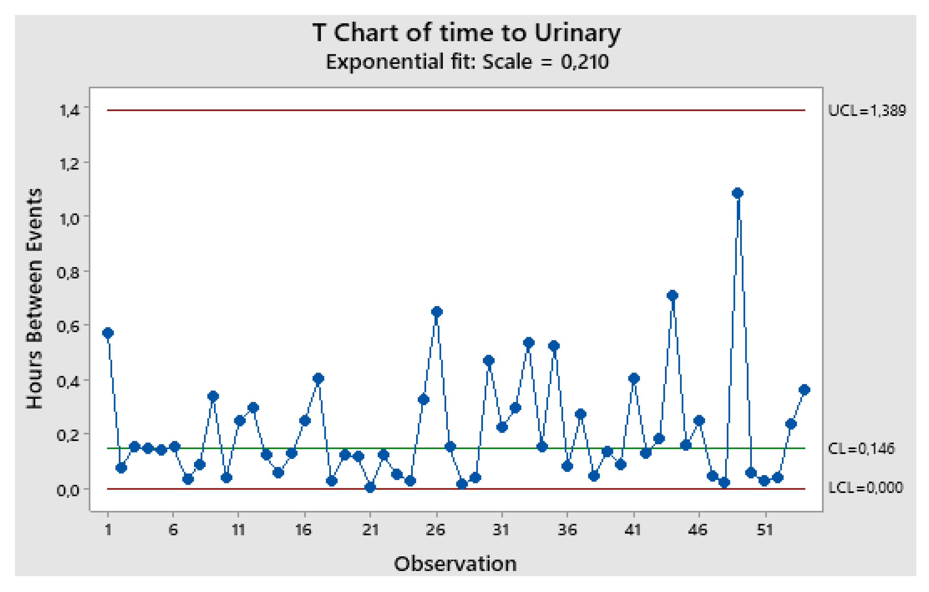
The analysis with JMP software, using the Rare Events Profiler, is in the Figure A1.
NOTICE that JMP, for Rare Events, Exponentially distributed, in the Figure A1, uses the Normal distribution! NONSENSE
It finds the UTI process OOC: both the charts, Individuals and Mobile Range are OOC.
The author informed the JMP User Community.
After various discussions, a member of the Staff (using the Exponential Distribution) provided the Figure A2.
You see that, now (Figure A2), the UTI process is IC: both the charts, Individuals and Mobile Range are IC; opposite decision than before (Figure A1), by the same JMP software (but with two different methods: the first is the standard method, while the second was devised by a JMP Staff member).
Figure A1.
First Control Chart by JMP.
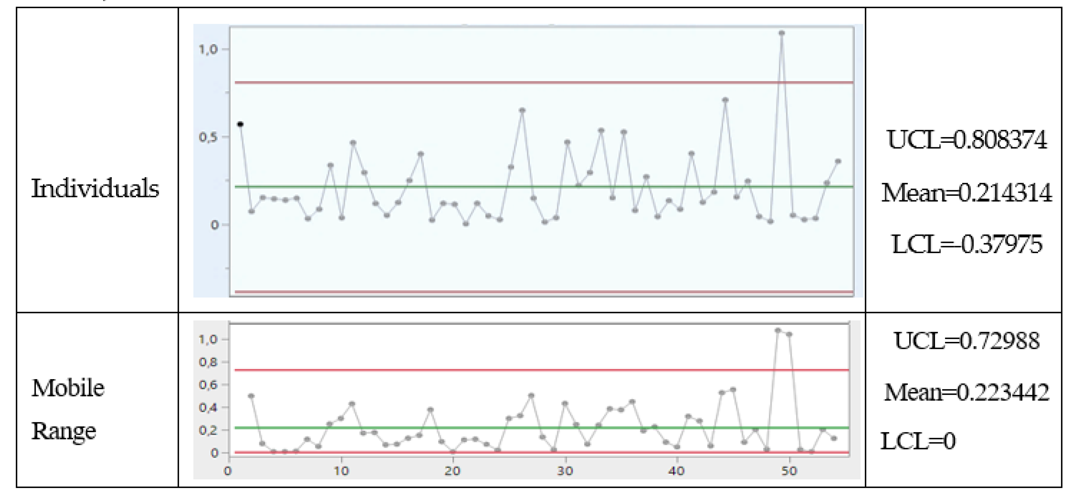
Figure A2.
Second Control Chart by a member of the Staff of JMP. Notice the numbers (LCL and UCL)!
Notice the LCL, the Mean and the UCL of both charts.
Compute the mean of all the data and you find a different value: therefore, the mean in the charts is not the mean of the process!
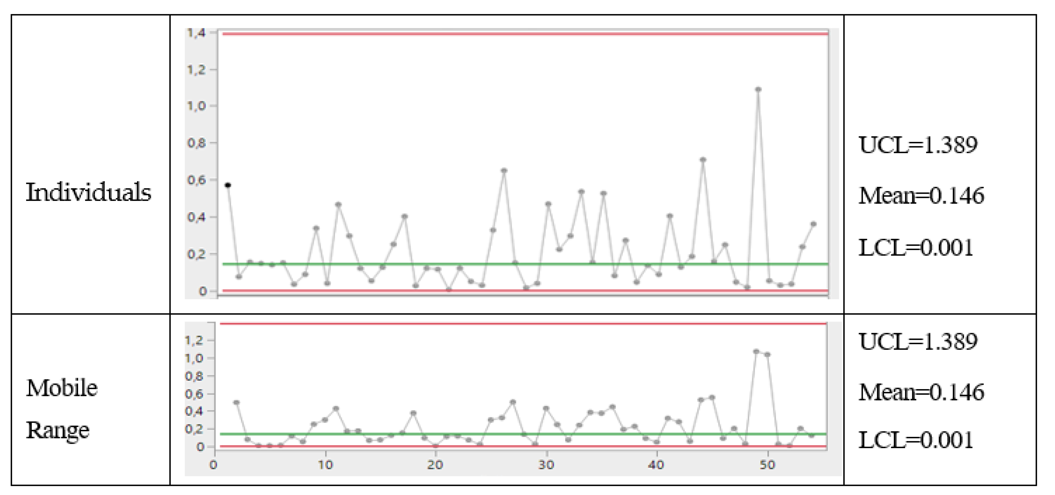
If one analyses the data with Minitab, he finds the Figure A3.
Figure A3.
Individual Control Chart by Minitab.
You see that now the UTI process is IC: notice the LCL, Mean and UCL.
A natural question arises: which of the three figures is correct?
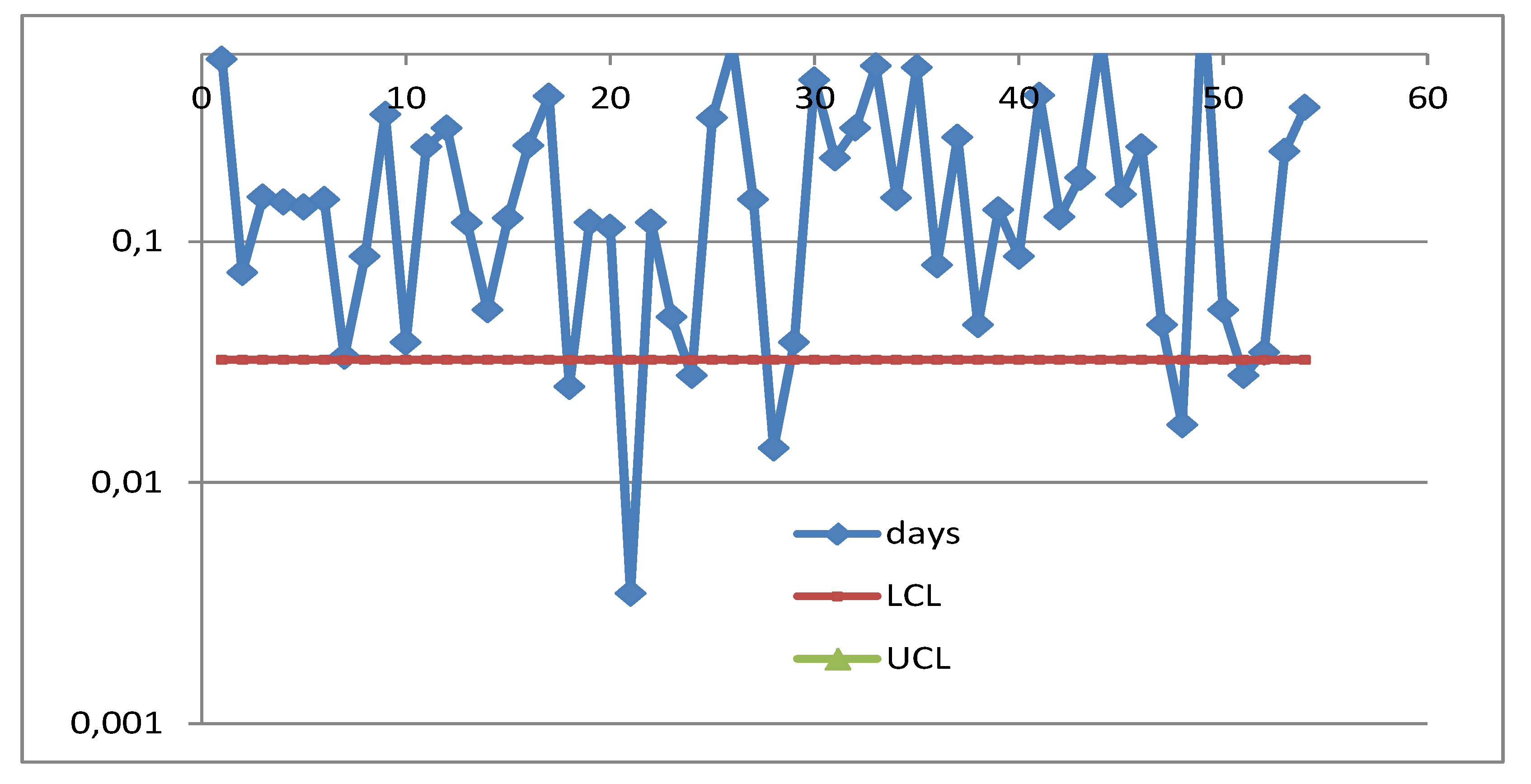
Actually, they all are wrong, as you can see from the Figure A4:
Figure A4.
Individual Control Chart by FG, using RIT: UTI process OOC.
The author offered JMP to become a better statistical software provider by solving the flaw according to JMP advertising:

No reaction … and therefore NO Corrective Action.
Appendix B
The Statistical Hypotheses and the Related Risks
We define as statistical hypothesis a statement about a population parameter (e.g. the ′′true′′ mean, the ′′true′′ shape, the ′′true′′ variance, the ′′true′′ reliability, the ′′true′′ failure rate, …). The set of all the possible values of the parameter is called the parameter space Θ. The goal of a hypothesis test is to decide, based on a sample drawn from the population, which value hypothesed for the population parameter of the parameter space Θ can be accepted as true. Remember: nobody knows the truth…
Generally, two competitive hypotheses are defined, the null hypothesis H0 and the alternative hypothesis H1.
If θ denotes the population parameter, the general form of the null hypothesis is H0: θ∈Θ0 versus the alternative hypothesis H1: θ∈Θ1, where Θ0 is a subset of the parameter space Θ and Θ1 a subset disjoint from Θ0. If the set Θ0={θ0, a single value} the null hypothesis H0 is called simple; on the contrary, the null hypothesis H0 is called composite. If the set Θ1={θ1, a single value} the alternative hypothesis H1 is called simple; on the contrary, the alternative hypothesis H1 is called composite.
In a hypothesis testing problem, after observing the sample (and getting the empirical sample of the data D) the experimenter (the Manager, the Researcher, the Scholar) must decide either to «accept» H0 as true or to reject H0 as false and then decide, on the opposite, that H1 is true.
Let’s make an example: let the reliability goal be [θ being the MTTF]; we ask the data D, from the reliability test to confirm the goal we set. Nobody knows the reality; otherwise, there would be no need of any test.
The test data D are the determinations of the random variables related to the items under test; it can happen then that the data, after their elaboration, provide us with an estimate far from (and therefore they induce us to decide that the goal has not been achieved).
Generally, in the case of reliability test, the reliability goal to be achieved is called null hypothesis .
The hypotheses are classified in various manners, such as (and some suitable combinations)
- Simple Hypothesis: it specifies completely the distribution (probabilistic model) and the values of the parameters of the distribution of the Random Variable under consideration
- Composite Hypothesis: it specifies completely the distribution (probabilistic model) BUT NOT the values of the parameters of the distribution of the Random Variable under consideration
- a. Parametric Hypothesis: it specifies completely the distribution (probabilistic model) and the values (some or all) of the parameters of the distribution of the Random Variable under consideration
- b. Non-parametric Hypothesis: it does not specify the distribution (probabilistic model) of the Random Variable under consideration
A hypothesis testing procedure (or simply a hypothesis test) is a rule (decision criterion) that specifies
- for which sample values the decision is made to «accept» H0 as true,
- for which sample values H0 is rejected and then H1 is accepted as true.
based on managerial/Statistics which defines
- the test statistic (a formula to analyse the data)
- the critical region R (rejection region)
to be used for decisions, with the stated risks: decision criterion.
The subset of the sample space for which H0 will be rejected is called rejection region (or critical region). The complement of the rejection region is called the acceptance region.
A hypothesis test of H0: θ∈Θ0 versus H1: θ∈Θ1, (Θ0∩Θ1=∅) might make one of two types of errors, traditionally named Type I Error and Type II Error; their probabilities are indicated as α and β.
Table B1.
Statistical Hypotheses and risks.
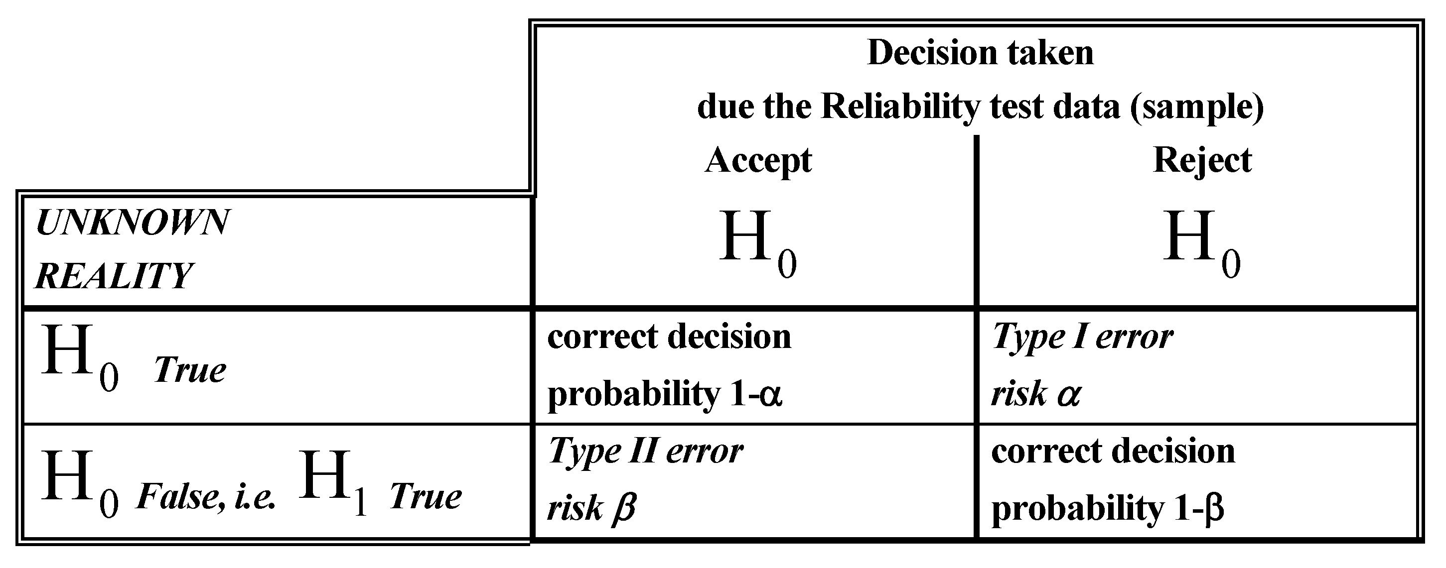
If «actually» H0: θ∈Θ0 is true and the hypothesis test (the rule), due to the collected data, incorrectly decides to reject H0 then the test (and the Experimenter, the Manager, the Researcher, the Scholar who follow the rule) makes a Type I Error, whose probability is α. If, on the other hand, «actually» θ∈Θ1 but the test (the rule), due to the collected data, incorrectly decides to accept H0 then the test (and the Experimenter, the Manager, the Researcher, the Scholar who follow the rule) makes a Type II Error, whose probability is β.
These two different situations are depicted in the previous table (for simple parametric hypotheses).
Notice that when we decide to “accept the null hypothesis” in reality we use a short-hand statement saying that we do not have enough elements to state the contrary.
It is evident that
Suppose R is the rejection region for a test, based on a «statistic s(D)» (the formula to elaborate the sampled data D).
Then for H0: θ∈Θ0, the test makes a mistake if «s(D)∈R», so that the probability of a Type I Error is α=P(S(D)∈R) [S(D) is the random variable giving the result s(D)].
It is important the power of the test 1-β, which is the probability of rejecting H0 when in reality H0 is false
Therefore, the power function of a hypothesis test with rejection region R is the function of θ defined by β(θ)=P(S(D)∈R). The function 1-power function is often named the Operating Characteristic curve [OC curve].
A good test has power function near 1 for most θ∉Θ0 and, on the other hand, near 0 and for most θ∈Θ0.
From a managerial point of view, it is sound using powerful tests: a powerful test (finds the reality and) rejects what must be rejected.
It is obvious that we want that the test be the most powerful and therefore one must seek for the statistics which have the maximum power; it’s absolutely analogous to the search of efficient estimators.
We know that the competition of simple hypotheses can have a good property: the most powerful critical region [i.e. the rejection region found has the highest power 1-β(θ)=P(S(D)∉R) of H1 against H0, for any α (α sometimes is called size of the critical region)]; a theorem regarding the likelihood ratio proves that.
Let’s define the likelihood ratio tests; let Θ denote the entire parameter space; the likelihood ratio test statistic for testing H0: θ∈Θ0 versus θ∈Θ1 is the ratio [which uses the Likelihood function L(θ|D)]
A likelihood ratio test is any test that has a rejection region that has the form {s(D): λ(D)≤c}, where c is any number satisfying 0≤c≤1 and s(D) is the “statistic” by which we elaborate the data of the empirical sample D. This test is a measure of how much the evidence, provided by the data D, supports H0.
The previous criterion is very simple if the two competing hypotheses are both simple: H0: θ=θ0 versus θ=θ1.
Let L0 be the Likelihood function L(θ0|D) and L1 be the Likelihood function L(θ1|D): the most powerful test is the one that has the most powerful critical region C={s(D): L1/L0≥kα}, where the quantity kα is chosen in such a way that the Type I Error has a risk (probability) α. The most powerful critical region C has the highest power 1-β(θ).
Usually when an efficient estimator exists, this provides then a powerful statistic, giving the most powerful test.
For the Normal model
the test about H0: θ∈Θ0 where is a given number, we get
where has the t distribution with n-1 degrees of freedom when H0 is true.
After some algebra, the test of H0 may be performed as follows: we compute the quantity and if
H0 is accepted; otherwise H0 is rejected.
It is worthwhile to observe that the Confidence Interval for is
Hence, the test of H0 is equivalent to the following points, for any distribution of the data:
- 1)
- Construct a confidence interval for the population mean
IF
- 2)
- THEN Accept H0; otherwise H0 is rejected.
This has great importance for Control Charts, as you can see in the figure
Figure B1.
LCL and UCL of Control Charts with their risks.
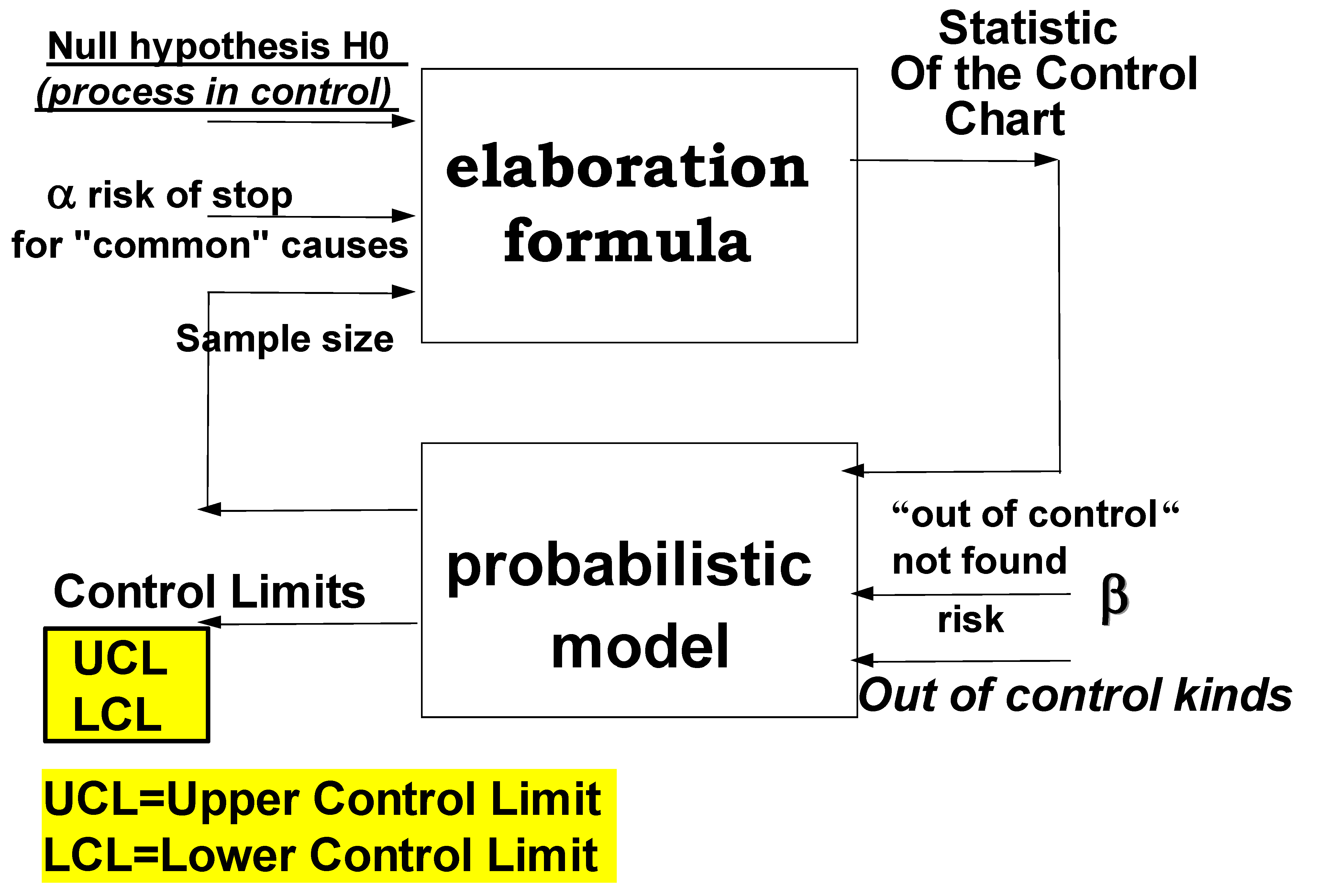
The good Managers, Researchers, Scholars do not forget that the two risks always are present and therefore they must take care of the power of the test 1-β, they use for the decision (as per the principles F1 and F2) [24,25,26,27,28,29,30].
Such Managers, Researchers, Scholars use the Scientific Method.
It is important to state immediately and in an explicit way that
- ⇒ the risks must be stated,
- ⇒ together with the goals (the hypotheses),
- ⇒ BEFORE any statistical (reliability) test is carried out.
For demonstration of reliability characteristics, with reliability tests, Managers, Students, Researchers and Scholars must take into account, according the F1 principle, the very great importance of W. E. Deming statements
- A figure without a theory tells nothing.
- There is no substitute for knowledge.
- There is widespread resistance of knowledge.
- Knowledge is a scarce national resource.
- Why waste Knowledge?
- Management need to grow-up their knowledge because experience alone, without theory, teaches nothing what to do to make Quality
- Anyone that engages teaching by hacks deserves to be rooked.
From these, unfortunately for Quality, for the Customers, for the Users and for the Society, this devastating result
- Ø The result is that hundreds of people are learning what is wrong. I make this statement on the basis of experience, seeing every day the devastating effects of incompetent teaching and faulty applications.
In many occasions and several Conferences on Total Quality Management for Higher Education Institutions, [Toulon (1998), Verona (1999), Derby (2000), Mons (2001), Lisbon (2002), Oviedo (2003), Palermo (2005), Paisley (2006), Florence (2008), Verona (2009)] the author (FG) showed many real cases, found in books and magazines specialized on Quality related to concepts, methods and applications wrong, linked to Quality [21–61]. All the very many documents published (more than 250) by F. Galetto show the profound truth that
facts and figures are useless, if not dangerous, without a sound theory (F. Galetto, 2000),
Brain is the most important asset: let’s not forget it. (F. Galetto, 2003),
All that is particularly important for the analysis of any type of data (quality or reliability).
Appendix C
Excerpt C1.
Typical statements in the “Garden …[24]” where the authors name LCL and UCL what actually are the Probability Limits L and U. See the Figure 9 and the Excerpt 12.
Excerpt C1.
Typical statements in the “Garden …[24]” where the authors name LCL and UCL what actually are the Probability Limits L and U. See the Figure 9 and the Excerpt 12.

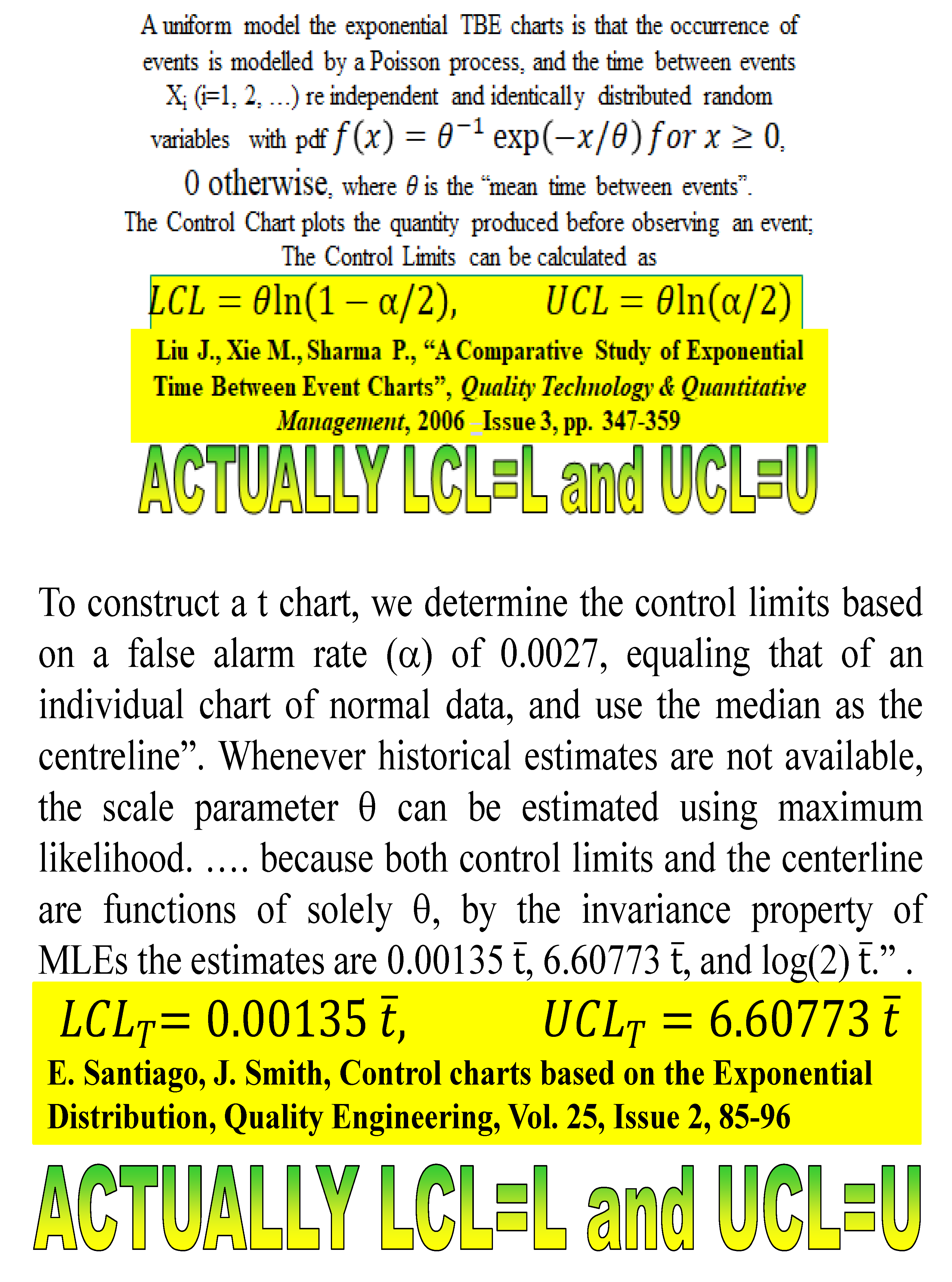
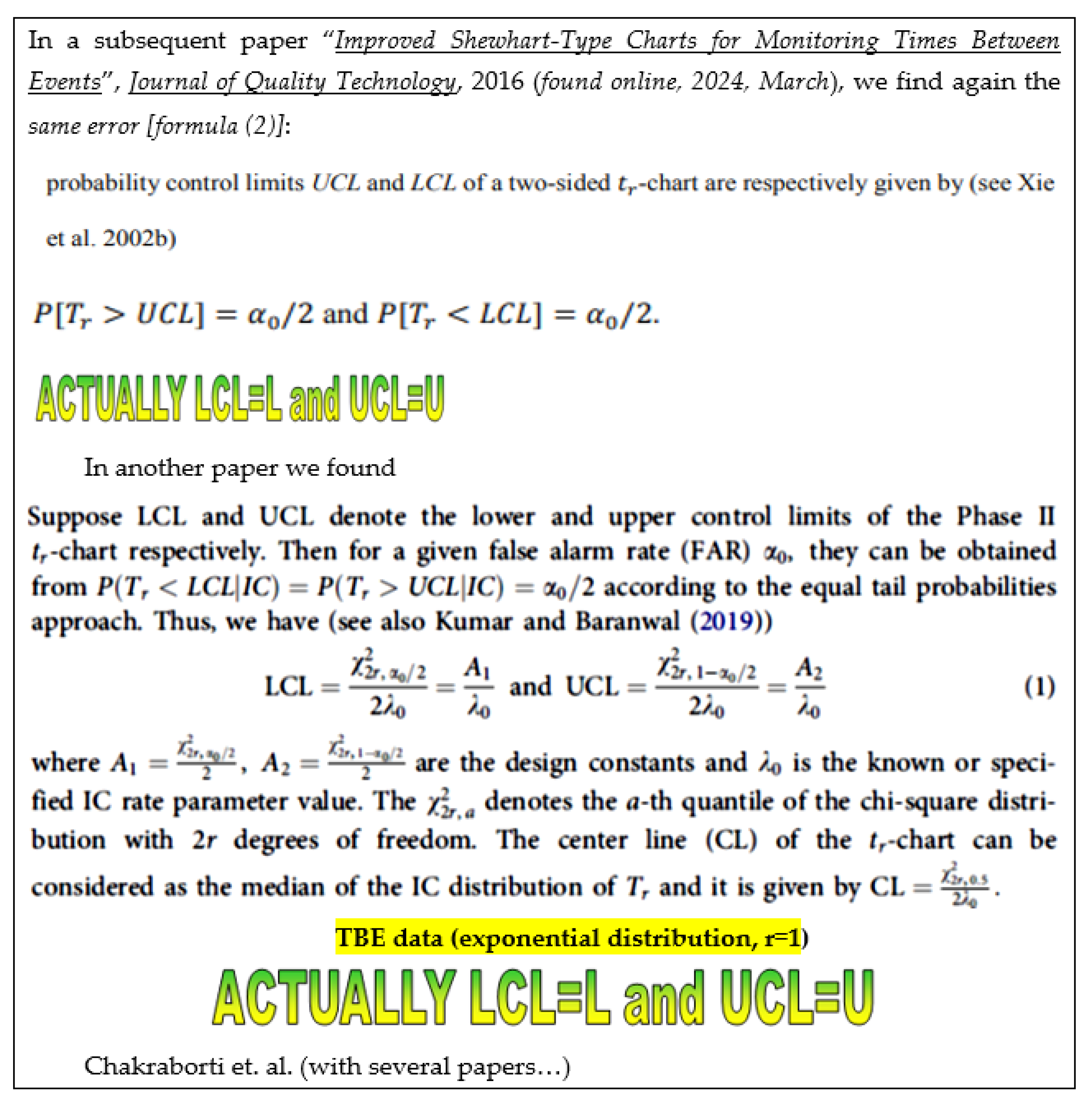
Many other cases, with the same errors, can be found in the “Garden …[24], and the Conclusions” where the authors name LCL and UCL what actually are the Probability Limits L and U.
References
References
- Galetto, F., Quality of methods for quality is important. European Organisation for Quality Control Conference, Vienna. 1989.
- Galetto, F., GIQA, the Golden Integral Quality Approach: from Management of Quality to Quality of Management. Total Quality Management (TQM), Vol. 10, No. 1; 1999.
- Chakraborti et al., Properties and performance of the c-chart for attributes data, Journal of Applied Statistics, January 2008.
- Kumar, N. , Chakraborti, S., Rakitzis, A. C. et al., Improved Shewhart-Type Charts for Monitoring Time Between Events. Journal of Quality Technology 2017, 49, 278–296. [Google Scholar] [CrossRef]
- Zhang, C. W. , Xie, M., Goh, T. N., Design of exponential control charts using a sequential sampling scheme. IIE Transactions 2006, 38, 1105–1116. [Google Scholar] [CrossRef]
- Belz, M. Statistical Methods in the Process Industry: McMillan; 1973.
- Casella, Berger, Statistical Inference, 2nd edition: Duxbury Advanced Series; 2002.
- Cramer, H. Mathematical Methods of Statistics: Princeton University Press; 1961.
- Deming W., E. , Out of the Crisis, Cambridge University Press; 1986.
- Deming W., E. , The new economics for industry, government, education: Cambridge University Press; 1997.
- Dore, P. , Introduzione al Calcolo delle Probabilità e alle sue applicazioni ingegneristiche, Casa Editrice Pàtron, Bologna; 1962.
- Juran, J. , Quality Control Handbook, 4th, 5th ed.: McGraw-Hill, New York: 1988-98.
- Kendall, Stuart, (1961) The advanced Theory of Statistics, Volume 2, Inference and Relationship:, Hafner Publishing Company; 1961.
- Meeker, W. Q. , Hahn, G. J., Escobar, L. A. Statistical Intervals: A Guide for Practitioners and Researchers. John Wiley & Sons. 2017. [Google Scholar]
- Mood, Graybill, Introduction to the Theory of Statistics, 2nd ed.: McGraw Hill; 1963.
- Rao, C. R. , Linear Statistical Inference and its Applications: Wiley & Sons; 1965.
- Rozanov, Y. , Processus Aleatoire, Editions MIR: Moscow, (traduit du russe); 1975.
- Ryan, T. P. , Statistical Methods for Quality Improvement: Wiley & Sons; 1989.
- Shewhart W., A. , Economic Control of Quality of Manufactured Products: D. Van Nostrand Company; 1931.
- Shewhart, W.A. , Statistical Method from the Viewpoint of Quality Control: Graduate School, Washington; 1936.
- D. J. Wheeler, Various posts, Online available from Quality Digest.
- Galetto, F., (2014), Papers, and Documents of FG, Research Gate.
- Galetto, F. , (2015-2025), Papers, and Documents of FG, Academia.
- Galetto, F. , (2024), The garden of flowers, Academia.
- Galetto, F. , Affidabilità Teoria e Metodi di calcolo: CLEUP editore, Padova (Italy); 1981-94.
- Galetto, F. , Affidabilità Prove di affidabilità: distribuzione incognita, distribuzione esponenziale: CLEUP editore, Padova (Italy); 1982, 85, 94.
- Galetto, F. , Qualità. Alcuni metodi statistici da Manager: CLUT, Torino (Italy; 1995-2010).
- Galetto, F. , Gestione Manageriale della Affidabilità: CLUT, Torino (Italy); 2010.
- Galetto, F. , Manutenzione e Affidabilità: CLUT, Torino (Italy); 2015.
- Galetto, F. , Reliability and Maintenance, Scientific Methods, Practical Approach, Vol-1: www.morebooks.de.; 2016.
- Galetto, F. , Reliability and Maintenance, Scientific Methods, Practical Approach, Vol-2: www.morebooks.de.; 2016.
- Galetto, F., Statistical Process Management, ELIVA press ISBN 9781636482897; 2019.
- Galetto F., Affidabilità per la manutenzione, Manutenzione per la disponibilità: tab edizioni, Roma (Italy), ISBN 978-88-92-95-435-9, www.tabedizioni.it; 2022.
- Galetto, F. Hope for the Future: Overcoming the DEEP Ignorance on the CI (Confidence Intervals) and on the DOE (Design of Experiments). Science J. Applied Mathematics and Statistics 2015, 3, 99–123. [Google Scholar] [CrossRef]
- Galetto, F. Management Versus Science: Peer-Reviewers do not Know the Subject They Have to Analyse. Journal of Investment and Management. 2015, 4, 319–329. [Google Scholar] [CrossRef]
- Galetto, F. The first step to Science Innovation: Down to the Basics. , Journal of Investment and Management. 2015, 4, 319–329. [Google Scholar] [CrossRef]
- Galetto, F. , (2021) Minitab T charts and quality decisions, Journal of Statistics and Management Systems. [CrossRef]
- Galetto, F., (2021) Control Charts for TBE and Quality Decisions, Academia.edu.
- Galetto, F. (2021) ASSURE: Adopting Statistical Significance for Understanding Research and Engineering, Journal of Engineering and Applied Sciences Technology, ISSN: 2634 – 8853, 2021 SRC/JEAST-128. [CrossRef]
- Galetto, F., (2006) Does Peer Review assure Quality of papers and Education? 8th Conference on TQM for HEI, Paisley (Scotland).
- Galetto, F., (2001), Looking for Quality in “quality books”, 4th Conference on TQM for HEI, Mons (Belgium).
- Galetto, F., (2001), Quality QFD and control charts, Conference ATA, Florence (Italy).
- Galetto, F., (2002), Fuzzy Logic and Control Charts, 3rd ICME Conference, Ischia (Italy).
- Galetto, F., (2010),The Pentalogy Beyond, 9th Conference on TQM for HEI, Verona (Italy).
- Galetto, F., (2024), News on Control Charts for JMP, Academia.edu.
- Galetto, F., (2024), JMP and Minitab betray Quality, Academia.edu.
Excerpt 1.
From the paper “Misguided Statistical Process Monitoring Approaches”.
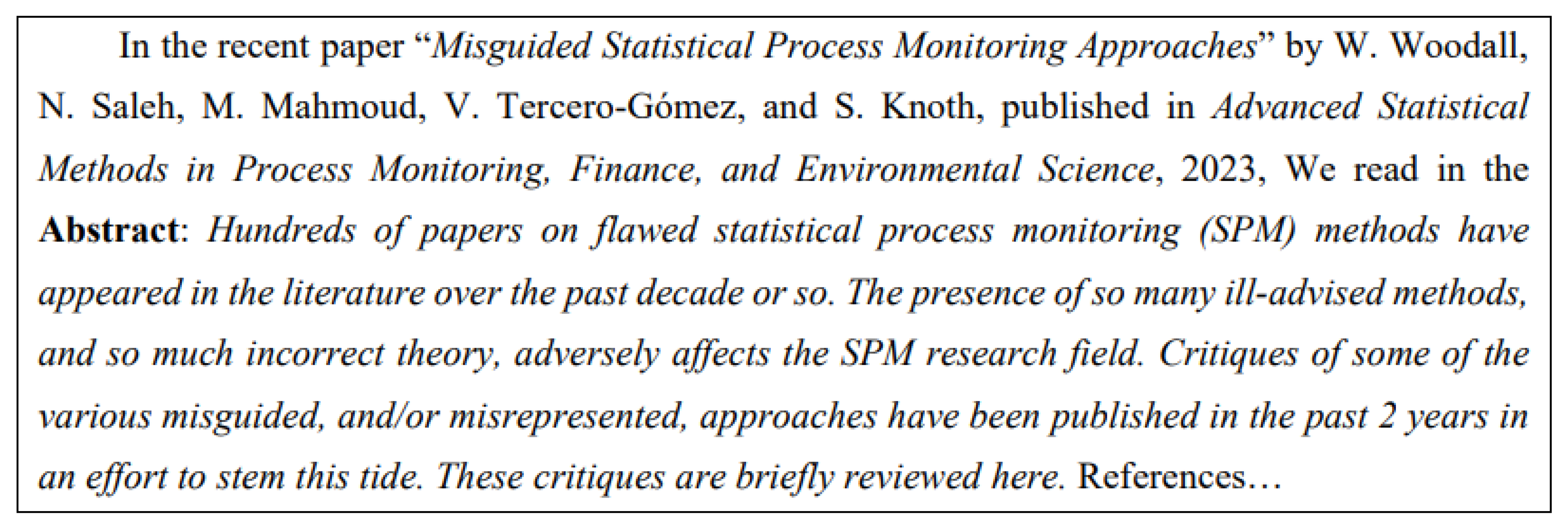
Figure 1.
Theoretical Difference between L------U and LCL------UCL.
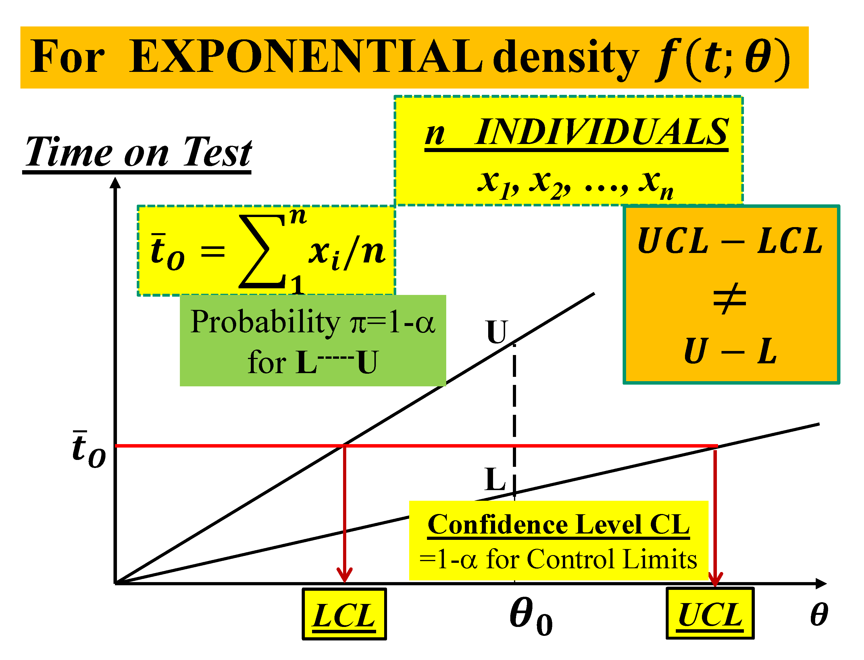
Excerpt 2.
Some statements of Deming about Knowledge and Theory (Deming 1986, 1997).
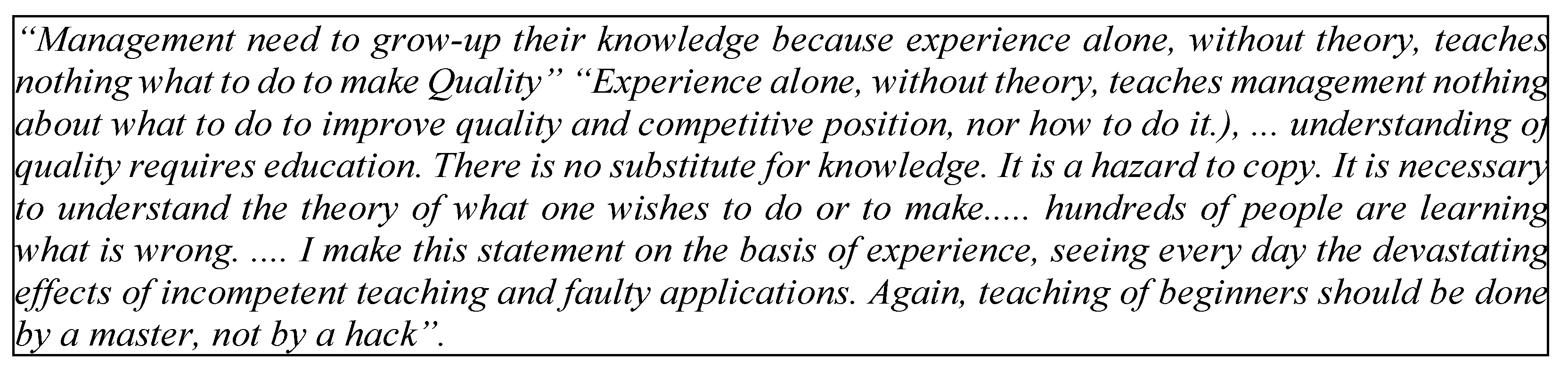
Excerpt 3.
From Shewhart book (1931), on page 294.

Excerpt 4.
From a paper in the “Garden… [24]”. Notice that one of the authors wrote several papers….
Excerpt 4.
From a paper in the “Garden… [24]”. Notice that one of the authors wrote several papers….

Figure 2.
Control Limits LCLX----UCLX=L----U (Probability interval), for Normal data (Individuals xij, sample size k) “sample means” and “grand mean”
Figure 2.
Control Limits LCLX----UCLX=L----U (Probability interval), for Normal data (Individuals xij, sample size k) “sample means” and “grand mean”
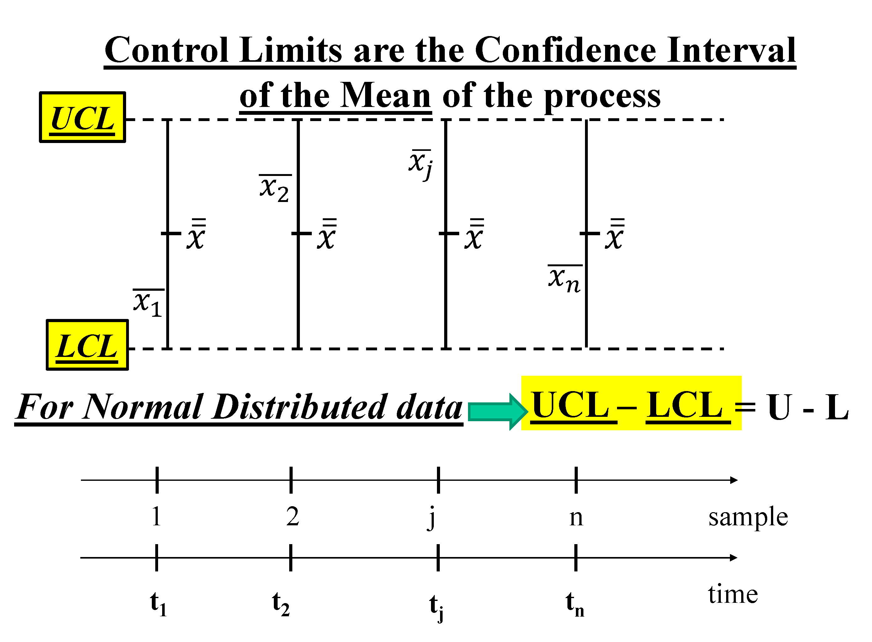
Figure 3.
Individual Control Chart (sample size k=1). Control Limits LCL----UCL=L----U (Probability interval), for Normal data (Individuals xi) and “grand mean”
Figure 3.
Individual Control Chart (sample size k=1). Control Limits LCL----UCL=L----U (Probability interval), for Normal data (Individuals xi) and “grand mean”
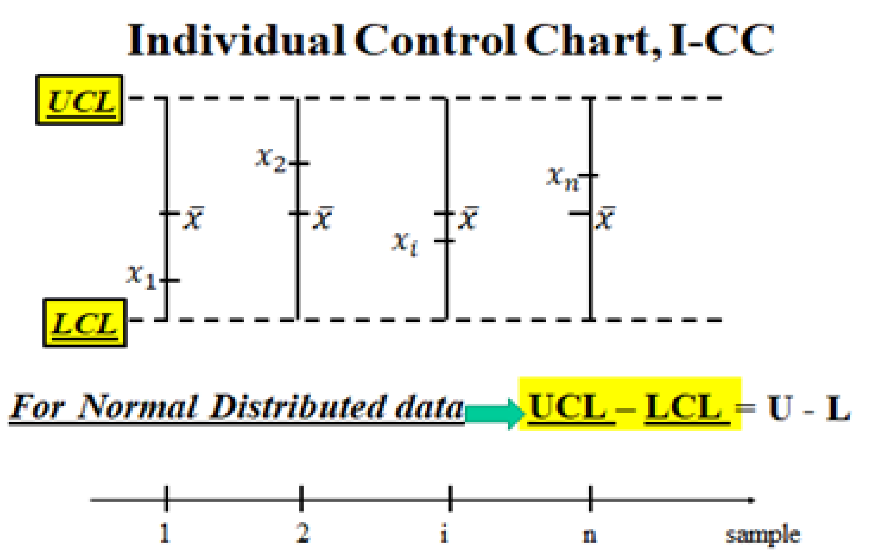
Figure 5.
Reliability of a “4 units Stand-by system” with MTTF=θ=123 days; is the total time on test of the 4 units. To compute the CI (with CL=0.8), find the abscissas of the intersections at and ….
Figure 5.
Reliability of a “4 units Stand-by system” with MTTF=θ=123 days; is the total time on test of the 4 units. To compute the CI (with CL=0.8), find the abscissas of the intersections at and ….
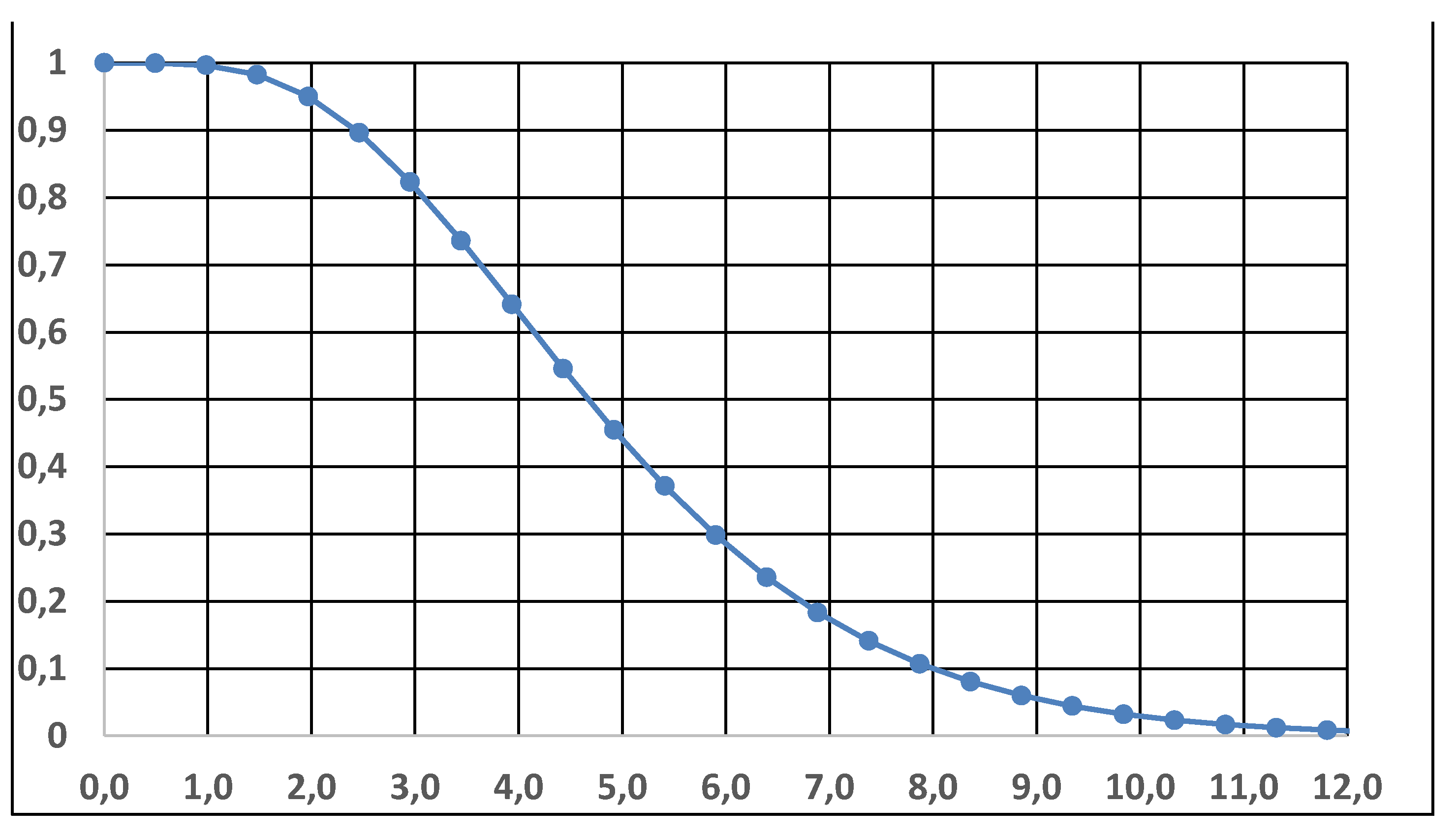
Figure 14.
Probability Interval L---U (vertical line) versus Random Intervals comprising the “mean” μ (horizontal random variable lines), for Normally distributed RVs .
Figure 14.
Probability Interval L---U (vertical line) versus Random Intervals comprising the “mean” μ (horizontal random variable lines), for Normally distributed RVs .
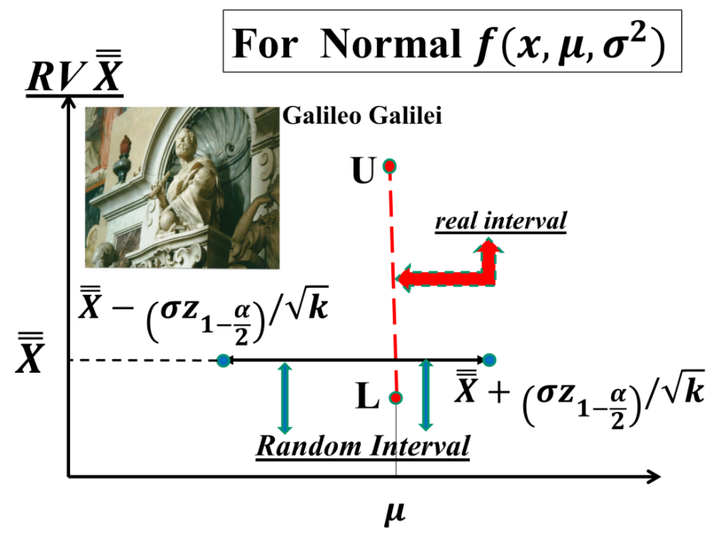
Table 3.
Estimation of the possible distributions for the 40 t4 and the Phase II 160 observations.
| Notice that only the Weibull … is Yes | Using 40 t4 data | Using 160 data | |||
| Exponential | NO | 924.02 | 231.13 | ||
| Weibull | Yes | 1.18 | 989.44 | 0.795 | 201.35 |
| Gamma | NO | 1.65 | 561.21 | 0.718 | 322.12 |
| Normal | NO | ||||
| Normal | NO | ||||
Disclaimer/Publisher’s Note: The statements, opinions and data contained in all publications are solely those of the individual author(s) and contributor(s) and not of MDPI and/or the editor(s). MDPI and/or the editor(s) disclaim responsibility for any injury to people or property resulting from any ideas, methods, instructions or products referred to in the content. |
© 2025 by the authors. Licensee MDPI, Basel, Switzerland. This article is an open access article distributed under the terms and conditions of the Creative Commons Attribution (CC BY) license (http://creativecommons.org/licenses/by/4.0/).
Copyright: This open access article is published under a Creative Commons CC BY 4.0 license, which permit the free download, distribution, and reuse, provided that the author and preprint are cited in any reuse.


