

Submitted:
14 September 2026
Posted:
15 September 2026
You are already at the latest version
Abstract
We develop an operational framework for testing small frequency-dependent departures from standard electromagnetic vacuum propagation. The vacuum is treated phenomenologically as a causal and passive linear-response system whose electromagnetic properties may exhibit weak spectral structure while preserving the reference vacuum impedance and recovering standard Maxwell behaviour at high frequency. A central feature of the framework is the separation between the hypothesized vacuum response and the spectral sensitivity of the measuring apparatus. Each experiment is represented by a calibrated sensitivity function, while its response is summarized by a corresponding band-averaged observable. This construction provides a common metrological interface through which different precision experiments can constrain the same underlying response model while retaining their instrument-specific calibration and uncertainty information. The proposed reporting scheme is intended to support reproducible cross-platform comparison and subsequent re-analysis for alternative admissible response models. First-order mappings are developed for resonant cavities, interferometric phase measurements, group delay, radiometry, and Casimir-type observables. For Casimir measurements, the analytically continued response and the experiment-dependent sensitivity are retained explicitly. A published optical-resonator constraint on the isotropic photon sector of the Standard-Model Extension is conditionally recast within the present framework, yielding an experimentally anchored sensitivity at approximately the ten-to-the-minus-eight level. The result is statistically consistent with zero and does not constitute evidence for a nontrivial vacuum response or a model-independent constraint on arbitrary dispersion. The framework is deliberately phenomenological rather than microscopic. It does not derive the vacuum degrees of freedom, the electromagnetic constants, the numerical value of the speed of light, or Lorentz symmetry. Its contribution is a causal, reproducible, and falsifiable interface between hypothetical vacuum-response models and precision photonic experiments, together with a candidate standardized metrological reporting structure for future cross-platform tests.
Keywords:
photonics
; electromagnetism
; optical resonators
; Casimir effect
; vacuum response
; precision measurements
; unificatie
; veldtheorie
; begrensd vacuüm
; emergentie
; analytische consistentie
; referentiekader
1. Introduction
Classical electrodynamics describes free space as a homogeneous, dispersionless background characterised by fixed electromagnetic parameters and a universal propagation speed [13,22]. From the quantum perspective, however, the vacuum is not physically featureless. Vacuum fluctuations and their boundary-dependent manifestations have observable consequences, most notably in Casimir phenomena [4,8,14,17]. This motivates a more specific phenomenological question: can a small residual electromagnetic response of the vacuum be formulated in a way that is physically admissible, quantitatively constrained, and directly testable?
The present work addresses that question through an effective “carried-light” picture. The terminology is intended operationally: electromagnetic propagation is described as responding to collective vacuum degrees of freedom, without assuming a specific microscopic mechanism for those degrees of freedom. The vacuum is therefore treated as an effective linear-response system whose possible departures from ideal Maxwell propagation can be parametrised and experimentally constrained.
The conceptual motivation comes from earlier bounded-vacuum models [15,16], in which a finite effective fluctuation ensemble was proposed as a possible physical origin of vacuum-energy bounds and an emergent electromagnetic response. Those earlier models motivate the present construction but are not re-derived here. In particular, the high-frequency condition introduced below,
is an admissibility condition on the operational response; it is not, by itself, a proof that the unrenormalized zero-point vacuum energy is finite. The present paper therefore separates the bounded-vacuum motivation from the experimentally testable response framework.
Related proposals have also connected the observed speed of light to the structure of quantum-vacuum fluctuations [36]. The present approach differs in emphasis by asking how such a hypothesis can be expressed as a causal, passive, and reproducible response model that can be confronted with precision photonic measurements.
Operational response.
We introduce a frequency-dependent retarded vacuum response and define its real-frequency dispersive component as
Within the scalar, impedance-invariant ansatz developed below, acts as an effective refractive response. Small departures from the Maxwell reference state are written as
The construction is deliberately phenomenological. It does not require a detailed microscopic model before experimental constraints can be formulated.
To compare different experiments, each measurement is associated with a calibrated spectral sensitivity function . For observables whose linear response can be represented by a real normalized sensitivity kernel,
and the corresponding band-averaged observable is
To first order,
Thus the instrument-specific spectral information remains encoded in , whereas provides a common quantity with which different platforms can report constraints on the same proposed vacuum response. Precision cavity and resonator experiments [1,9,37], radiometric measurements [5,24,33], and Casimir experiments [3,10,23,28,34] provide representative experimental settings in which such band-dependent constraints can be formulated.
More general signed or complex transfer functions can be treated by the corresponding generalized linear-response kernel; the unit-area scalar form is the baseline used throughout this paper. Figure 1 summarizes this operational pipeline.
Physical admissibility.
The response is required to satisfy three basic conditions. First, it must be causal. We therefore formulate the underlying response as a retarded function that is analytic in the upper half of the complex plane. Its real and imaginary components are consequently linked by the Kramers–Kronig relations [13,22]. Second, the response is taken to be passive. With the Fourier convention used here, this requires
so that the effective response does not act as an unmodelled source of electromagnetic energy. This is consistent with the standard linear-response and fluctuation–dissipation framework [6,20,21]. Third, the modification must disappear asymptotically,
thereby recovering the Maxwell high-frequency limit. In this paper the term Casimir-safe refers specifically to preservation of the standard ultraviolet electromagnetic behaviour and compatibility with precision Casimir constraints [4,17,29]. It does not mean that the bare vacuum energy has been rendered finite.
Impedance-invariant construction.
A central requirement is that the parametrisation itself should not generate artificial reflection effects. We therefore co-scale the effective electric and magnetic responses according to
which leaves their ratio unchanged:
This construction modifies the effective propagation constant while preserving the reference vacuum impedance. Standard electromagnetic response theory provides the relevant framework for such dispersive quantities [13,22]. The impedance invariance should not be interpreted as implying that the electromagnetic stored-energy density remains unchanged in a dispersive medium. Correct energy accounting generally involves frequency derivatives of the constitutive response, as discussed in Appendix A and in standard treatments of dispersive electrodynamics [22].
Experimental scope.
The framework is developed for several classes of precision measurements: resonant cavities, interferometric phase measurements, time-of-flight or group-delay measurements, calibrated radiometry, and Casimir-type observables. Representative high-sensitivity cavity and optomechanical platforms are described in [1,9,37]; calibrated radiometric methods are exemplified by [5,24,33]; and the present experimental and theoretical Casimir landscape is represented by [3,4,10,17,23,28,29,34].
These platforms are not presented as independent applications of an established microscopic theory. Their role is to show how the same hypothetical vacuum response could be falsified or bounded through different experimental sensitivity functions. For radiometric applications we conservatively leave source spectra unchanged unless an explicit microscopic matter–field coupling model is supplied. This is consistent with treating thermal fluctuations and dissipation through the established fluctuation–dissipation framework [6,20,21] and with calibrated radiometric practice [5,24,33]. Likewise, in cavity and interferometric mappings the apparatus geometry and material reference standards are treated as fixed calibration inputs. A theory in which the same vacuum response also modifies those matter-sector references would require an enlarged coupled model and lies outside the present scope.
The scalar response is isotropic only in the frame in which it is specified. The present work therefore does not infer Lorentz invariance from spectral flatness. Possible frame-dependent signatures are treated separately, while any derivation of observer-independent Lorentz symmetry from microscopic vacuum dynamics remains an open problem.
Reproducibility and cross-platform comparison.
The usefulness of depends on retaining the instrument information encoded in . We therefore advocate publication of the calibrated sensitivity function together with the derived , its uncertainty budget, and the processing information needed to reproduce the integration. Such reporting follows established principles of open and reproducible computational research [30,31,35,38]. This separation between the experimental window and the assumed vacuum response permits an archived dataset to be re-evaluated for alternative admissible forms of without reconstructing the complete apparatus model.
Scope and contribution.
The purpose of this paper is therefore deliberately limited. We do not claim to derive the microscopic vacuum, the exact numerical value of c, the electromagnetic constants, or Lorentz symmetry. Instead, we construct a physically admissible operational interface between a bounded-vacuum hypothesis and measurable photonic observables. The principal contributions are:
- 1.
- a causal, passive, and impedance-invariant retarded response with a Maxwell high-frequency limit;
- 2.
- a real-frequency operational window ;
- 3.
- a calibrated band observable that separates instrument sensitivity from the assumed vacuum response;
- 4.
- first-order mappings to cavity, interferometric, delay, radiometric, and Casimir-type observables; and
- 5.
- a standardized metrological reporting framework in which the calibrated sensitivity function , the derived band observable , calibration information, and the associated uncertainty budget are published together, enabling reproducible cross-platform comparison and re-analysis for alternative admissible response models [30,31,35,38].
The proposed reporting structure should not be interpreted as implying a universal instrument response. Each experimental platform retains its own calibrated sensitivity function , reflecting its actual spectral weighting and transfer characteristics. What is common across platforms is instead the metrological representation:
In this sense, the – construction is intended not only as an observable for the present vacuum-response phenomenology, but also as a candidate common metrological interface for future cross-platform tests of weak frequency-dependent electromagnetic propagation effects.
This common representation provides a standardized interface through which independent experiments can constrain the same pre-specified response while preserving their instrument-specific information.
A fully calibrated sensitivity function may therefore serve as a reference response window for a particular experimental class, but not as a universal sensitivity function for all instruments. The universality proposed here lies in the normalization, calibration, uncertainty treatment, and reporting convention rather than in the specific spectral shape of .
The central question is consequently not whether the present phenomenology already establishes a microscopic bounded vacuum, but whether a residual response of this form is compatible with existing measurements and can be constrained more tightly by future ones. The remainder of the paper develops that falsifiable operational framework.
2. Operational Interface for Falsifiability
The role of , , and is purely operational: to render the conceptual proposal empirically testable and reportable.
We model the vacuum as linear, isotropic and homogeneous with a single scalar response (“window”) that co-scales the electromagnetic parameters while preserving the wave impedance:
so that remains constant and no spurious boundary-impedance effects are introduced [13,22]. We adopt the notation convention
and use it consistently throughout.
Operational response factor and free-space reference.
The proposed frequency-dependent response factor makes the concept of a fluctuating quantum vacuum operational. It represents the collective influence of vacuum fluctuations without modelling their microscopic details individually, thus describing how the vacuum behaves as an effective medium for electromagnetic propagation.
The construction of follows three fundamental requirements:
- Causality — the response to an electromagnetic excitation must occur only after the stimulus itself; in the frequency domain this leads to the Kramers–Kronig relations linking the real and imaginary parts of the retarded response.
- Passivity — the vacuum cannot act as an unmodelled energy source; with the adopted convention, for positive frequencies.
- Free-space limit — at very high frequencies the influence of the fluctuating background vanishes and the full retarded response approaches unity, recovering the ideal Maxwell reference state.
Free space thus acts as a reference state: it defines the zero-deviation baseline against which the frequency-dependent properties of the fluctuating vacuum are measured. Whenever , the model allows the speed, phase, and group structure of electromagnetic waves to differ slightly from the Maxwell reference.
2.1. Low-energy Parametrization of Dispersion in
At sufficiently low energies, gapless transverse modes with approximately linear dispersion can arise in effective descriptions that approach a Maxwell-like regime. Higher-order operators may then generate small momentum-dependent corrections to the leading linear propagation law.
As an illustrative low-energy parametrisation, consider
where is dimensionless and denotes an effective momentum scale.
Using
the frequency-dependent part of the effective refractive response is, to leading order, quadratic in frequency.
A distinction is required, however, between the total low-frequency response and its dispersive variation. For a general causal and passive response satisfying
the low-frequency real part need not satisfy . We therefore write
where
is the zero-frequency offset and
The sign of the zero-frequency offset is further constrained by causality and passivity. Under the usual reality, regularity, and convergence conditions for the retarded response, the Kramers–Kronig relation evaluated at zero frequency gives
For the passive convention adopted here,
and therefore, provided that the integral in Eq. (19) exists,
Thus, within the causal passive response class considered here, the zero-frequency offset is not an arbitrary signed parameter. A strictly positive offset is expected whenever the absorptive part has nonzero positive spectral weight. The equality is possible only when the corresponding weighted absorptive contribution vanishes.
This statement applies to the zero-frequency limit of the full causal response. It should not be confused with an approximately constant response over a finite experimental band, which will be denoted when required below.
For the quadratic effective expansion above,
with
Accordingly, the complete low-energy response may be written as
for frequencies sufficiently below the effective scale .
The constant term and the dispersive curvature represent different experimental signatures. A sufficiently narrowband experiment may be primarily sensitive to their combination, whereas measurements over separated frequency bands or measurements of spectral slope can, in principle, distinguish a constant offset from a frequency-dependent component.
If the constant component has been independently calibrated, removed, or constrained separately, the remaining dispersive observable is
For the quadratic parametrisation,
where
An upper limit on the dispersive component therefore implies
This bound is explicitly model dependent. It applies only to the quadratic low-energy residual of Eq. (22) and should not be interpreted as a model-independent determination of a microscopic vacuum scale.
Equation (24) is a low-frequency effective expansion and does not specify the ultraviolet completion of the response. In particular, the condition
must be imposed on the full causal retarded response and cannot be inferred from the truncated low-energy series.
The sign of is left open and must ultimately be determined by an underlying microscopic completion or by experiment. Likewise, no specific relation between , , and the parameters of the causal single-pole response introduced below is assumed.
To make the causal structure explicit, we therefore distinguish the low-energy expansion from a separate global response model. A minimal single-pole example is
whose only pole lies at
On the real-frequency axis,
and
Thus
while
and the real and imaginary components satisfy the Kramers–Kronig relations.
Its low-frequency expansion is
Equation (36) illustrates explicitly why a causal passive response may contain both a constant low-frequency offset and a quadratic dispersive curvature. After subtraction of the constant offset, the leading frequency-dependent term is quadratic, as in Eq. (22). No quantitative identification between the coefficients of the two parametrisations is assumed without an explicit microscopic matching calculation.
2.2. Minimal Consistency Conditions
The operational response introduced above is required to satisfy a minimal set of consistency conditions before it can be confronted with precision measurements.
(i) Casimir-safe ultraviolet limit.
The response must recover the standard Maxwell behaviour at sufficiently high frequency,
or, equivalently on the real-frequency axis,
This condition ensures that the proposed modification becomes asymptotically negligible and introduces no additional ultraviolet growth relative to standard electromagnetic theory. In the restricted sense used throughout this work, this is what is meant by “Casimir-safe.” It does not imply that the unrenormalized zero-point vacuum energy has been rendered finite. The distinction is consistent with the standard theoretical and experimental treatment of the Casimir interaction [4,17,29].
(ii) Causality and passivity.
The underlying retarded response is required to be analytic in the upper half of the complex plane. With the Fourier convention adopted here, passivity requires
(iii) Small-deviation regime.
We write
and linearize the observable mappings unless stated otherwise. For the purely numerical worked examples below, amplitudes of order – may be used to make the spectral response clearly visible and to test the numerical integration procedure. These values are illustrative only and are not intended to represent experimentally allowed frequency-independent vacuum-response amplitudes.
Band observable.
For a calibrated real-frequency sensitivity function , normalized according to
we define the common cross-platform reporting quantity
Using , one obtains to first order
where
A positive corresponds, under the convention , to an effective increase of the refractive response and hence to a decrease of the phase-propagation speed relative to the Maxwell reference value. Accordingly, a positive band-averaged gives a negative .
Concrete causal baseline.
Unless stated otherwise, the numerical worked example uses the real part of the causal single-pole response introduced in Section 2.1,
with
Its real-frequency dispersive component is
The associated imaginary part is fixed by the same retarded response and is therefore not specified independently. Throughout the real-frequency analysis we use Eq. (41) and Eq. (45). For Casimir observables the response is instead evaluated on the imaginary-frequency axis and a logarithmic measure is used, as specified in Section 3.5.
3. Mappings to Experimental Observables
Below we give first-order mappings (), keeping careful track of signs and connecting to .
3.1. Resonant Frequency Shifts (Cavities)
3.2. Interferometric Phase (Fixed Laser Frequency)
For arm-difference L at angular frequency , . Thus at fixed , , and band-averaged
3.3. Time-of-Flight and Group Delay
For a weakly absorptive response, the real propagation constant is
The local group velocity is therefore
For propagation over a distance L, with
the first-order fractional group-delay shift is
This observable is therefore sensitive not only to the local magnitude of the refractive response but also to its spectral slope.
The constant offset contributes to phase and delay but not to the frequency derivative. For the quadratic residual
one has
and therefore
By comparison, the corresponding fixed-frequency phase shift is approximately
Thus, within this quadratic low-energy model,
so that a combined phase–delay measurement can in principle suppress sensitivity to the constant offset and isolate the dispersive component.
For broadband measurements the corresponding quantities must be averaged with the calibrated experimental transfer functions. A bound on the quadratic effective scale follows only from a constraint on the dispersive component, as discussed in Section 6.4.
3.4. Radiometry: Calibrated Propagation Response
Radiometric measurements provide a complementary way to constrain a frequency-dependent propagation response, but the mapping from to a measured band power is generally instrument dependent. We therefore do not assume that the fractional power shift is equal directly to .
In the conservative treatment adopted here, the source spectrum is held fixed. Thus a blackbody, Johnson-noise source, or calibrated radiometric reference is described by its standard source spectrum, while sensitivity to the proposed vacuum response enters through the propagation and instrumental transfer functions. This separation is consistent with standard calibrated radiometric practice [5,11,24,33] and avoids introducing an additional matter–vacuum coupling that is not specified by the present model.
Let the detected band power be written schematically as
where is the calibrated source spectrum and represents the complete propagation, detector, and readout transfer function. For a small departure , the measured power can be expanded to first order about the Maxwell reference state:
with
The kernel is an experimentally calibrated linear-response quantity. It contains the frequency dependence of the optical or microwave path, coupling efficiency, detector response, filtering, and readout calibration. In general it need not be positive at every frequency.
If
we define the normalized radiometric sensitivity window
Using the band observable
the first-order power response becomes
for the propagation-only model. Thus characterizes the spectral deformation, whereas describes how strongly the particular radiometric platform converts that deformation into a measured fractional power shift. The simpler relation is recovered only in a convention or calibration for which ; it is not assumed universally.
Source-sector extensions.
The present treatment deliberately keeps fixed. A microscopic model in which the same vacuum response also modifies thermal emission, Johnson noise, atomic transition strengths, or other source properties would introduce an additional first-order term,
Such a source contribution should be represented by its own calibrated response kernel and reported separately from the propagation kernel. Combining source and propagation effects without an explicit coupling model would risk double counting. The fluctuation–dissipation theorem provides the standard relation between equilibrium fluctuations and dissipative response [6,20,21], but it does not by itself specify how the bounded-vacuum response modifies a material source. That question therefore remains outside the scope of the present operational model.
3.5. Casimir-Type Observables
Casimir measurements provide a complementary way to constrain the proposed vacuum response. In contrast to the real-frequency propagation observables considered above, the Lifshitz formulation is naturally expressed on the imaginary-frequency axis. We therefore define
where is the analytic continuation of the retarded response and is not an independent response function.
For a given Casimir configuration, the first-order fractional force response can be written in the general linear-functional form
where is the complete Casimir sensitivity kernel. The kernel is platform dependent. In general it contains both the explicit change of the propagation factor across the gap and any first-order change of the TE and TM reflection amplitudes induced by the modified gap response. Its detailed form therefore depends on the plate materials, separation, temperature, polarization, geometry, and calibration model. A compact derivation from the Lifshitz free energy is given in Appendix E.
Unlike the positive unit-area baseline used for some real-frequency examples, need not be positive at every frequency. We therefore first define the total Casimir sensitivity factor
provided that . The corresponding normalized Casimir sensitivity function is then
so that
In analogy with the real-frequency band observable, we define
Substituting the normalized kernel into Eq. (71) gives
to first order.
Thus characterizes the spectral deformation sampled by the Casimir experiment, whereas specifies how strongly that particular experimental configuration converts the deformation into a measurable fractional force shift. The simpler relation is recovered only in a convention for which the overall sensitivity has already been absorbed into the kernel so that ; it is not assumed generally.
The relevant response is the analytically continued quantity rather than a bare real-frequency vacuum-energy spectrum. Consistency with the standard ultraviolet structure requires
or equivalently . This condition does not render the unrenormalized zero-point energy finite. Rather, it ensures that the proposed deformation becomes asymptotically negligible and that the standard electromagnetic ultraviolet structure of the Lifshitz interaction is recovered. Consequently, the term “Casimir-safe” is used here in the restricted sense of ultraviolet compatibility and consistency with precision Casimir measurements. A quantitative bound on the vacuum response requires the actual geometry, material response functions, temperature, plate separation, calibration model, and uncertainty budget of the experiment. Once these are specified, the corresponding , , and can be constructed and used to constrain admissible forms of .
4. Comparison with Existing Tests and Frameworks
4.1. Isotropic SME Mapping
The isotropic photon sector of the Standard-Model Extension (SME) provides a useful comparison framework for an effectively frequency-independent modification of electromagnetic propagation. We adopt the photon-sector notation and convention of Kostelecký and Mewes [18], with the broader SME coefficient conventions summarized in [19].
In the minimal isotropic photon sector, the electromagnetic constitutive response may be written, to leading order, as
Hence
and the corresponding refractive index is
Within the present phenomenological framework,
Therefore, when the isotropic SME contribution is effectively constant over the experimental bandwidth and both descriptions are interpreted within the same photon-sector reference convention,
Using the operational definition , the corresponding band-averaged relation becomes
If is frequency independent over the instrument band, this reduces to
Thus a positive corresponds, in this convention, to , an effective refractive index greater than unity, and therefore a reduced phase-propagation speed relative to the Maxwell reference value.
This correspondence should be interpreted with care. In the full SME, isotropic photon-sector effects are defined relative to the matter-sector standards used by the experiment. Coordinate and field redefinitions can redistribute isotropic Lorentz-violating effects between photon and matter sectors [18,19]. Experimental constraints therefore apply to relative propagation effects with respect to the material rods, clocks, resonators, or particle sectors that define the measurement standard, rather than to an absolute photon-sector coefficient in isolation.
The mapping above is consequently a comparison between two effective descriptions under a common reference convention. It does not imply that the vacuum-response function is microscopically identical to an SME coefficient, nor that the present bounded-vacuum phenomenology constitutes an SME model.
4.2. Band-Averaged SME Correspondence and Dispersive Response
The minimal isotropic photon-sector coefficient is ordinarily treated as frequency independent within the minimal SME. The leading-order relation
therefore applies directly only when the effective refractive deformation is approximately constant over the relevant experimental bandwidth and the same reference-sector convention is used.
For a general weak response over a finite experimental band, it is useful to separate an approximately constant component from a genuinely frequency-dependent component:
For the specific low-energy expansion of Sec. 2.1, the constant term is the zero-frequency offset
More generally, over a finite experimental band, an effectively frequency-independent contribution is denoted .
Using the normalized sensitivity function,
the total band response becomes
Defining
one obtains
to first order.
The distinction is important experimentally. A single narrowband measurement generally constrains the combination in Eq. (90); it does not by itself determine whether the measured response arises from a constant offset or from dispersion. Measurements in separated frequency bands, or direct measurements of spectral slope, can provide the additional information required to separate the two contributions.
If an SME-like frequency-dependent comparison quantity is introduced phenomenologically through
then
Such a frequency-dependent quantity must not be identified without qualification with the constant coefficient of the minimal SME. It is only an effective comparison function unless an explicit matching to a dispersive or nonminimal SME model is supplied.
The quadratic low-energy parametrisation introduced in Section 2.1 applies specifically to the offset-subtracted dispersive component,
It follows that
where
Consequently, a constraint on the dispersive band component gives
This relation is not an SME bound. It follows specifically from the quadratic dispersive parametrisation. A constraint on the total can be inserted into Eq. (96) only if the constant contribution has been independently removed, calibrated, or shown to be negligible.
For reproducibility, experimental results should therefore report the calibrated sensitivity function, its normalization and effective band edges, the measured total response, and, where possible, the separately inferred constant and dispersive components.
4.3. Placement Within the Experimental Landscape
Expressing results as isolates apparatus details in and enables cross-band meta-analysis once is published. Representative settings include optical and microwave cavities [1,9,37], radiometry [5,11,24,33], and Casimir platforms [3,4,10,17,23,28,29,34]. We recommend reporting together with machine-readable for re-integration [30,31,35,38].
Scope and conservative assumption.
In this work we treat radiometric sources (blackbody/Johnson) as standard, i.e. their spectra are not modified by in the absence of a microscopic matter–field coupling model. Sensitivity to W enters through propagation and calibrated transfer functions only, consistent with fluctuation–dissipation theory [6,20,21] and radiometric practice [5,11,24,33]. This prevents double counting and keeps results immediately comparable across platforms. Models that directly alter source spectra fall outside the present scope but could be accommodated by publishing the corresponding source window alongside .
4.4. Isotropy and Frames
The scalar response used here is isotropic in the frame in which it is specified. Identifying that frame phenomenologically with, for example, the CMB rest frame does not by itself provide a transformation law for .
As an illustrative estimate only, suppose that a small boost with speed changes the sampled frequency primarily through the usual first-order Doppler shift. A frequency-dependent response would then generate a directional modulation of order
For a decomposition over the relevant experimental band,
the constant component does not contribute to the spectral derivative. To first order in the small response,
For a quadratic dispersive residual,
this becomes
An orbital boost of order would therefore produce, under these illustrative assumptions, a modulation of order
The band-constant component does not contribute to this leading spectral-slope signal. A quantitative prediction, however, requires an explicit transformation law for the complete retarded response and for the matter-sector quantities used as experimental frequency and length standards. The estimate above is therefore not used as evidence for the model.
5. Implications and Extensions
5.1. Fluctuation–Dissipation Connection
Within the conservative treatment adopted here, thermal source spectra are retained in their standard blackbody or Johnson-noise form, while sensitivity to the proposed vacuum response enters through propagation and calibrated transfer functions. This is a modelling assumption in the absence of an explicit microscopic matter–vacuum coupling model and is consistent with standard calibrated radiometric practice [5,33].
The fluctuation–dissipation theorem constrains the relation between equilibrium fluctuations and dissipative response [6,20,21], but it does not by itself specify how the phenomenological vacuum response modifies a material source. Any microscopic model in which the same vacuum response alters blackbody emission, Johnson noise, atomic transition strengths, or other source-sector properties would therefore require an additional source-response kernel and should be treated separately from the propagation response to avoid double counting.
5.2. Casimir-Safe Ultraviolet Behaviour
The high-frequency condition
does not render the unrenormalized zero-point vacuum energy finite. Rather, it ensures that the proposed bounded-vacuum modification becomes asymptotically negligible and that the standard Maxwell ultraviolet behaviour is recovered.
Accordingly, the term “Casimir-safe” is used here in the restricted sense that the response introduces no additional ultraviolet growth relative to the standard electromagnetic vacuum. The physically measurable Casimir interaction remains defined through the usual subtraction or renormalization of configuration-independent vacuum contributions [4,8,17,25,26].
For a small deformation,
the relevant Casimir correction is governed by the analytically continued response
rather than by a bare real-frequency vacuum-energy integral. As derived in Section 3.5 and Appendix E, the complete first-order fractional force response for a given experimental configuration may be written as
where is the full experiment-specific Casimir sensitivity kernel.
The kernel contains the geometry-, material-, polarization-, temperature-, separation-, and calibration-dependent response of the experiment. In general it contains both the explicit modification of the propagation factor across the gap and the corresponding first-order changes of the TE and TM reflection amplitudes. This structure follows the standard Lifshitz treatment of electromagnetic fluctuations between material boundaries [4,17,25,26,27].
When
we define the normalized sensitivity function
The corresponding Casimir band observable is
Substituting gives
The distinction between and is essential. The normalized quantity characterizes the spectral deformation sampled by the experiment, whereas specifies how strongly the particular configuration converts that deformation into a measurable fractional force shift. The proportionality factor can be omitted only if it has already been absorbed into the definition of the response kernel.
The ultraviolet consistency requirement is
or equivalently . This requirement preserves the established high-frequency structure of the Lifshitz interaction while allowing finite, frequency-dependent departures at lower frequencies to be constrained by precision Casimir measurements [3,10,23,28,29,34]. A viable response must therefore satisfy both the ultraviolet condition and existing experimental limits on Casimir-force residuals. Quantitative constraints require the actual geometry, material response functions, temperature, separation, calibration model, and uncertainty budget of the selected experiment.
Thus “Casimir-safe” denotes ultraviolet compatibility and consistency with precision Casimir phenomenology; it does not constitute a regularization of the bare vacuum energy and does not by itself imply agreement with a specific Casimir experiment.
5.3. Spectral Representations
A convenient causal positive-kernel representation is
Each kernel has its pole in the lower half-plane, has non-negative loss for , and tends to zero as . Positive superpositions therefore preserve causality, passivity, and the Maxwell high-frequency limit by construction.
5.4. Astrophysical and Cosmological Connections
Astrophysical and cosmological observations probe electromagnetic propagation over frequency ranges, path lengths, and epochs that are inaccessible to laboratory experiments. They may therefore provide complementary constraints on a frequency-dependent vacuum response .
The cosmic microwave background is particularly relevant because its spectrum is measured with high precision and its propagation extends over cosmological distances [11,32]. However, the observed limits on CMB spectral distortions or temperature anisotropies cannot be translated directly into a bound on without specifying how the response enters cosmological photon propagation.
Such a mapping would in general require a model for the redshift evolution of the response,
together with the corresponding modification of photon phase, frequency transport, arrival time, intensity transfer, or other observable quantities along the line of sight. The resulting cosmological observable would then have the schematic linear-response form
where is an observable-specific cosmological transfer kernel. Only after this kernel has been derived for a particular observable can an effective band quantity analogous to be defined and compared consistently with laboratory constraints.
Accordingly, the CMB measurements cited here should be regarded as potential external consistency tests rather than as direct limits. The present paper does not derive the required cosmological transfer law and therefore does not assign a numerical CMB bound to . The principal role of astrophysical observations in the present framework is consequently prospective: a causal response that is compatible with laboratory measurements should ultimately also be tested against long-baseline and cosmological propagation once its redshift dependence and coupling to the relevant observables have been specified.
5.5. Relation to Bounded-Vacuum Energy Models
The phenomenological response framework developed here is motivated in part by earlier bounded-vacuum models, in which the physically realized vacuum spectrum is assumed not to contribute uniformly over arbitrarily large frequency or energy scales [15,16]. Related discussions in the literature have also considered possible connections between vacuum fluctuations, electromagnetic propagation, and gravitationally relevant vacuum energy [7,36].
The present work does not derive the response function from those models. Instead, it asks a more restricted question: if the electromagnetic vacuum possesses a small residual frequency-dependent response, what properties must that response have in order to be compatible with causal propagation and precision measurement?
Accordingly, the bounded-vacuum picture and the operational response should be kept conceptually distinct. The former provides a possible physical motivation for expecting a nontrivial spectral structure, whereas the latter is a phenomenological object that can be constrained experimentally without assuming a particular microscopic origin. In particular, the ultraviolet condition as does not imply that the bare zero-point energy is rendered finite. Its role in the present framework is only to ensure that the proposed electromagnetic modification disappears asymptotically and that the standard Maxwell high-frequency limit is recovered.
A quantitative connection between a bounded vacuum-energy spectrum and the response would require an additional microscopic derivation. Such a derivation would have to specify how the underlying vacuum degrees of freedom generate the effective electromagnetic constitutive response and, if cosmological applications are intended, how that response evolves with the background state or redshift.
The operational framework presented here should therefore be regarded as a testable intermediate layer:
Only the final two stages are developed quantitatively in the present paper. Establishing the preceding microscopic connection remains a separate theoretical problem.
6. Discussion and Relation to Previous Work
The framework developed in this work should be interpreted at two distinct levels. At the conceptual level, it is motivated by the possibility that electromagnetic propagation reflects collective properties of the quantum vacuum. At the operational level, which is the principal subject of the present paper, that possibility is represented by a causal retarded response and tested through the band-averaged observable .
Maintaining this distinction is important. The present construction does not provide a microscopic derivation of the vacuum degrees of freedom, the numerical value of the speed of light, the electromagnetic constants, or Lorentz symmetry. Instead, it asks a more restricted and experimentally accessible question: if a small residual electromagnetic vacuum response exists, what conditions must it satisfy, and how can different precision measurements constrain it in a common language?
6.1. Relation to Bounded-Vacuum Models
The phenomenological motivation originates in earlier bounded-vacuum models by the author [15,16]. Those works explored the possibility that an effective physical bound on the vacuum fluctuation spectrum could yield a finite effective vacuum-energy density and could be related to large-scale electromagnetic and cosmological behaviour.
The present work does not rederive those results. In particular, the condition for should not be interpreted as a regularisation of the bare zero-point energy. As discussed in Section 5.2, its role here is narrower: it ensures that the proposed modification becomes asymptotically negligible and that the standard Maxwell ultraviolet behaviour is recovered.
The bounded-vacuum picture therefore serves as a motivation for the existence of a nontrivial response function, whereas the response framework itself can be tested independently of the detailed mechanism that may ultimately generate it. Related work has also proposed connections between vacuum fluctuations and the observed propagation speed of light [36]. The present formulation differs by concentrating on the response-theory requirements that make such a proposal empirically admissible: causality, passivity, impedance preservation, ultraviolet recovery of Maxwell electrodynamics, and explicit sensitivity-weighted observables.
6.2. Operational Content of the Response
The central phenomenological object is the retarded response , with the real-frequency dispersive window . For the impedance-invariant construction,
so that . This co-scaling is a phenomenological choice designed to isolate propagation effects without introducing artificial impedance mismatch. It is consistent with standard dispersive electromagnetic response theory [13,22], but it should not be interpreted as a microscopic derivation of or .
Causality requires to be analytic in the upper half of the complex frequency plane, while passivity requires a non-negative absorptive component for positive frequency under the Fourier convention adopted here. These requirements place dispersion and absorption within a single response function rather than allowing them to be varied independently. This is consistent with the standard linear-response and fluctuation–dissipation framework [6,20,21]. The single-pole response introduced in Section 2.1 provides one explicit example satisfying these conditions. It is used as a causal baseline, not as a unique microscopic model of the vacuum.
6.3. Cross-platform Interpretation of
The main practical result of this work is the separation between the hypothesised vacuum response and the spectral sensitivity of a specific measurement. For a normalized real sensitivity kernel ,
The experimental apparatus is therefore represented by , while the assumed physics is represented by . This separation makes it possible, in principle, to reanalyse the same experimental sensitivity for different admissible response models.
The first-order mappings derived in Section 3 illustrate how this construction can be applied to several distinct experimental classes. Representative cavity and resonator platforms include [1,9,37]; calibrated radiometric measurements are represented by [5,24,33]; and precision Casimir measurements and their theoretical interpretation are described in [3,4,10,17,23,28,29,34].
These references do not constitute measurements of itself. Rather, they identify experimental methodologies from which an appropriate sensitivity kernel could be constructed. A direct constraint on the present framework requires the corresponding instrument response, calibration model, and uncertainty budget to be specified explicitly. More general experiments may require signed or complex response kernels rather than the positive unit-area scalar baseline adopted here. In such cases the same logic extends naturally to the appropriate linear transfer functional.
6.4. From a Dispersive Band Constraint to an Effective Scale
For an experimental band in which the slowly varying part of the response may be approximated as frequency independent, we write
For the specific low-energy expansion of Sec. 2.1, the corresponding constant term is
with
The corresponding dispersive band quantity is
To leading order,
where
An experimental upper limit on the magnitude of the dispersive component therefore implies
The distinction between and is essential. Since
for the low-energy decomposition, a limit on the total band response does not by itself determine if the band-constant contribution is unknown.
A numerical scale bound therefore requires either an independent constraint on , a calibration procedure that removes the constant component, or measurements across multiple bands that isolate the spectral curvature. Setting is an additional model assumption and should be stated explicitly if adopted.
The scale has dimensions of angular frequency. A characteristic length such as
is only an effective dimensional correspondence. Neither nor should be interpreted as a model-independent microscopic vacuum scale without an underlying microscopic derivation.
6.5. Casimir Constraints and Ultraviolet Behaviour
Casimir experiments provide a particularly useful consistency test because they probe the electromagnetic response through its analytic continuation to the imaginary-frequency axis. The relevant theoretical framework is the Lifshitz formulation and its extensions to realistic materials [4,17,25,26,29]. Within the present framework, the condition as ensures that the proposed deformation does not introduce additional ultraviolet growth relative to standard electrodynamics. Existing Casimir measurements [3,10,23,28,34] therefore constrain admissible forms of once the full geometry-, material-, and temperature-dependent sensitivity is taken into account.
The term Casimir-safe is used in precisely this restricted sense. It denotes compatibility with the standard ultraviolet asymptotics and with precision Casimir constraints; it does not imply that the unrenormalized electromagnetic vacuum energy has become finite.
6.6. Frame Dependence and Lorentz Symmetry
A frequency-dependent scalar response requires specification of the frame in which the frequency argument is defined. In the present phenomenological construction, is therefore understood with respect to a homogeneous and isotropic effective rest frame. This does not constitute a violation signal by itself, nor does spectral flatness establish Lorentz invariance. A quantitative comparison between different inertial frames would require an explicit transformation law for the complete response, including any matter-sector quantities used as clocks or length references. For this reason, the boost estimate given above is treated only as an illustrative possible signature. The stronger question of whether a microscopic bounded-vacuum theory can recover observer-independent Lorentz symmetry remains open and is separated from the operational results of the present paper.
6.7. Relation to Reproducible Experimental Practice
An advantage of the – formulation is that it makes the assumptions entering a constraint explicit. Publishing the sensitivity kernel, its normalization, the calibration chain, uncertainty budget, frequency grid, and analysis code permits a result to be independently reproduced and subsequently re-evaluated for alternative admissible response functions. This approach is consistent with established recommendations for open and reproducible computational research [30,31,35,38]. The framework therefore does not require different experiments to adopt the same microscopic interpretation. It requires only that each experiment state sufficiently clearly how its measured quantity weights the proposed response.
6.8. Limitations and Interpretation
Several limitations should be kept explicit. First, the framework is phenomenological. A causal and passive defines an admissible response, but it does not explain why that response exists. Second, the present mappings treat apparatus geometry, material properties, and reference standards as fixed calibration inputs unless otherwise stated. A microscopic theory in which the same vacuum dynamics modifies matter-sector properties would require a coupled analysis. Third, the low-energy EFT expansion and the causal single-pole response are not identified with one another. They represent complementary parameterisations at different descriptive levels, and any quantitative matching between them requires an explicit microscopic calculation. Fourth, the present work does not establish a cosmological propagation law. Observations such as the CMB temperature and spectrum [11,24,32] may eventually provide complementary constraints, but only after a model has been specified that relates along cosmological propagation to the observed spectrum. Finally, analyticity, passivity, and ultraviolet normalisation define an admissible class of response functions but do not establish dynamical attraction toward that class. Claims of self-organisation, fixed points, or emergent fundamental laws require additional dynamics and are therefore left as open questions.
6.9. Prospective Falsification Tests
The operational framework developed here permits several complementary routes toward direct falsification of a specified vacuum-response model. The relevant requirement is stronger than obtaining a single bound on : one and the same pre-specified causal response should remain compatible with independent measurements performed with different spectral sensitivities and, where applicable, with its analytic continuation to imaginary frequency.
A first test is a multi-band resonator comparison. Precision cavity and resonator experiments operating at well-separated carrier frequencies can be assigned distinct calibrated sensitivity functions , yielding
Measurements in microwave and optical bands would therefore constrain the same at substantially different frequencies. Such comparisons are particularly useful for distinguishing an approximately band-independent contribution from genuine spectral curvature. Representative high-precision cavity and resonator methodologies are discussed in Refs. [1,9,37], while the optical-resonator result used in Appendix G provides one concrete experimental benchmark [2].
A second and potentially more selective test combines fixed-frequency phase measurements with group-delay measurements. As shown in Sec. 3.3, for the quadratic low-energy residual considered here,
The frequency-independent contribution cancels at leading order, so that the difference directly probes the dispersive component of the response. A combined phase–delay experiment can therefore provide a cleaner constraint on spectral curvature than a single band-averaged measurement alone.
A third test follows directly from causality. The dispersive and absorptive components of are not independent, but are linked by the Kramers–Kronig relations. Consequently, a response model that predicts an observable real-frequency dispersion must also possess the corresponding absorptive structure required by the same analytic retarded response. Independent limits on loss and dispersion therefore provide an internal consistency test of the proposed within standard linear-response theory [6,13,20,21,22].
A fourth and qualitatively independent test is provided by Casimir measurements. These probe the analytically continued response
through the Lifshitz interaction rather than through real-frequency propagation. As developed in Sec. 3.5 and Appendix E, a quantitative comparison requires the complete experiment-specific Casimir sensitivity kernel, including material response, geometry, separation, temperature, polarization, calibration, and uncertainty information. Precision Casimir experiments can therefore test whether a response that remains compatible with real-frequency photonic measurements also remains admissible on the imaginary-frequency axis [3,4,10,17,23,28,29,34].
The strongest test of the framework would combine these independent constraints. For a response family with parameters fixed or fitted according to a predefined protocol, define the admissible parameter regions obtained from the separate experimental classes as
The specified response model is excluded if no common parameter region remains,
at a predefined statistical confidence level and with shared systematic uncertainties treated consistently.
This provides a concrete falsification criterion: the same causal response must simultaneously satisfy separated-frequency propagation tests, phase–delay consistency, dispersion–absorption consistency, and Casimir constraints. Conversely, consistency across these independent observables would not by itself establish a microscopic vacuum model, but would identify a surviving phenomenological response class for further experimental and theoretical investigation.
6.10. Overall Interpretation
The contribution of the present work is consequently narrower, but also more directly falsifiable, than a microscopic theory of the quantum vacuum. It provides a controlled interface
Within that interface, the bounded-vacuum concept supplies physical motivation, whereas causality, passivity, impedance preservation, and the Maxwell ultraviolet limit define admissibility. Precision experiments then determine how large any residual response is allowed to be. A future microscopic theory would have to explain why a response of this class arises, how its parameters are fixed, how matter-sector references transform with it, and whether Lorentz symmetry and the observed electromagnetic constants can emerge consistently. Those questions remain beyond the claims of the present paper.
7. Conclusions
This work has developed an operational framework for testing small frequency-dependent departures from standard electromagnetic vacuum propagation. The central phenomenological object is the causal retarded response , with experimentally accessible real-frequency dispersive component
The construction is formulated within standard linear-response and dispersive electromagnetic theory [6,13,20,21,22].
For a calibrated real-frequency sensitivity function , normalized according to , the corresponding operational band quantity is
As developed in Section 2.2, the principal operational result of the paper is the separation between the hypothesized vacuum response and the spectral sensitivity of the measurement. The assumed physics is contained in , whereas the experiment-specific weighting is contained in . The quantity therefore provides a common cross-platform reporting variable without erasing the instrument dependence contained in the sensitivity function itself.
The impedance-invariant ansatz and preserves the reference electromagnetic impedance while allowing a dispersive propagation response. This co-scaling is a phenomenological choice consistent with standard electromagnetic response theory [13,22]; it is not a microscopic derivation of or . Causality requires to be analytic in the upper half of the complex frequency plane, while passivity constrains its absorptive component. The real and imaginary parts of the response are therefore linked through the Kramers–Kronig structure rather than being independent phenomenological inputs [6,20,21,22].
The additional high-frequency requirement as ensures recovery of the Maxwell ultraviolet limit. As discussed in Secs. Section 3.5 and Section 5.2, this is the restricted meaning of “Casimir-safe” adopted in this work: the proposed deformation introduces no additional ultraviolet growth into the electromagnetic response and can be incorporated consistently into the standard Lifshitz description of Casimir observables [4,8,17,25,26,29]. It does not imply that the unrenormalized zero-point vacuum energy has been rendered finite [14].
The first-order mappings developed in Section 3 for resonant cavities, interferometric phase, group delay, radiometry, and Casimir-type measurements show that should not in general be identified directly with a measured fractional shift. Each experimental platform has its own calibrated response or sensitivity kernel. Representative precision platforms include optical and microwave resonators [1,9,37], calibrated radiometric measurements [5,24,33], and precision Casimir experiments [3,10,23,28,29,34].
For radiometric and Casimir observables in particular, an additional platform-dependent sensitivity factor is generally required to convert the weighted vacuum response into the measured fractional signal. For the Casimir case this gives
as derived in Section 3.5 and Appendix E.
The comparison with the isotropic photon sector of the Standard-Model Extension provides a concrete bridge to existing precision measurements. In the conventional photon-sector description [18,19], and under the corresponding reference-sector and transformation assumptions, the leading-order comparison for an effectively frequency-independent isotropic response is
This identification is conditional. In the SME, isotropic photon-sector coefficients are defined relative to the matter-sector standards used by the experiment, and coordinate or field redefinitions can redistribute isotropic Lorentz-violating effects between sectors [18,19]. The present vacuum-response framework should therefore not be interpreted as being microscopically identical to the SME.
As demonstrated in Appendix G, the optical-resonator result of Baynes, Luiten, and Tobar [2] can nevertheless be recast conditionally as
with the approximate Gaussian envelope
The result is statistically consistent with zero and therefore does not constitute evidence for a nonzero vacuum response. It is not a new measurement of , but an SME-conditioned translation of an existing precision-photonic constraint. Related resonator measurements provide complementary limits on isotropic photon-sector deviations [12].
Extending Eq. (132) to a genuinely frequency-dependent requires the calibrated spectral sensitivity function of the experiment, together with its uncertainty and the appropriate transformation law. The published SME coefficient alone is insufficient to provide a model-independent exclusion curve for an arbitrary dispersive vacuum response.
The causal single-pole response introduced in Section 2.1 illustrates how such instrument information can be converted into a constraint on a particular causal response model. As shown in Appendix G.6,
and therefore, for ,
A numerical exclusion curve consequently requires the actual experimental sensitivity function rather than the published band constraint alone.
Similarly, the quadratic low-energy parametrisation introduced in Section 2.1 provides a model-dependent relation between a measured band constraint and an effective scale . As emphasized in Section 4.2 and Appendix G.7, this interpretation is distinct from the dispersionless isotropic SME correspondence and should not be regarded as an SME bound unless an explicit microscopic matching relation is supplied.
Astrophysical and cosmological observations may eventually provide complementary constraints over frequency ranges and propagation distances inaccessible to laboratory experiments. High-precision CMB measurements by COBE/FIRAS and Planck provide particularly stringent tests of electromagnetic propagation [11,24,32]. However, these observations cannot be converted directly into bounds on without an explicit model for the redshift evolution and cosmological transfer of . They are therefore treated here as prospective consistency tests rather than as numerical constraints on the present framework.
The construction developed in this paper remains phenomenological. It does not derive the microscopic vacuum degrees of freedom, , , the numerical value of c, Lorentz symmetry, or the response function itself. Earlier bounded-vacuum models by the author provide physical motivation for considering a nontrivial spectral structure [15,16], while other work has independently explored possible connections between quantum vacuum fluctuations and electromagnetic propagation [36]. These motivations do not constitute a microscopic derivation of the present response.
The logical structure of the present work is therefore
Only the stages from to measurable constraints are developed quantitatively in the present work. The microscopic-response mechanism remains to be derived independently.
The next experimental step is therefore concrete: for a selected precision platform, determine or reconstruct the calibrated sensitivity kernel, propagate its uncertainty, and use it to obtain a frequency-dependent exclusion curve for an admissible causal response. Publication of the corresponding sensitivity kernel and calibration information would also permit independent re-integration for alternative response models, consistent with established principles of reproducible computational research [30,31,35,38].
The complementary theoretical task is to determine whether a microscopic bounded-vacuum model can generate an admissible while simultaneously satisfying causality, passivity, electromagnetic precision constraints, Casimir limits, and the required matter-sector reference conventions.
The main result of this work is consequently neither a detection of a bounded vacuum nor a derivation of an emergent speed of light. It is a falsifiable operational framework that specifies how a hypothetical small vacuum response can be formulated consistently, connected conditionally to existing precision-photonic measurements, and subjected to progressively stronger experimental tests.
Acknowledgments
AI-assisted language and analytical tools, including ChatGPT (OpenAI), were used during manuscript preparation to assist with language refinement, structural organization, mathematical consistency checks, and presentation. All scientific assumptions, derivations, interpretations, numerical results, references, and final conclusions were reviewed and approved by the author, who takes full responsibility for the content of the manuscript. No AI system is listed as an author.
Appendix A. Wave Propagation and Causal Retarded Response
We collect here the wave-propagation relations associated with the impedance-invariant co-scaling ansatz for and , and make the causal structure of the vacuum response explicit.
For real-frequency propagation it is useful to distinguish the full complex retarded response from the real operational window used in the band-averaged observables of the main text. Using the Fourier convention , we identify
for the phase-sensitive real-frequency measurements considered here. The imaginary part of describes the corresponding absorptive component required by a causal linear response.
Complex wave number.
For the co-scaling ansatz
the refractive response on the branch continuously connected to vacuum is . The complex wave number is therefore
With the adopted Fourier convention, passivity requires for , so that a wave proportional to is attenuated rather than amplified during propagation.
Phase velocity and group delay.
In a weakly absorptive frequency interval, the phase velocity associated with the real propagation constant is
For a sufficiently narrow pulse whose distortion remains small across the relevant bandwidth, the local group delay and corresponding local group velocity are
Writing with , the corresponding first-order relations are
These expressions reproduce the real, weak-loss limit used in the main-text phase and time-delay mappings.
Importantly, the local group velocity is not by itself a fundamental criterion for relativistic causality. In strongly dispersive or absorptive regions, may exceed c or even become negative without implying superluminal transmission of information. The relevant causal requirement is instead the analytic structure of the retarded response together with its high-frequency asymptotic behaviour [13,22].
Illustrative causal single-pole response.
To make the causal structure explicit, we use a complex retarded response rather than specifying only a real dispersion curve. A minimal illustrative example is
The response has a single pole at , which lies in the lower half of the complex plane. Hence is analytic in the upper half-plane, as required for a retarded causal response under the Fourier convention adopted here.
Defining , its real and imaginary components are
For and , , so the illustrative response is passive. Moreover, for , and the Maxwell response is recovered asymptotically.
Because the real and imaginary components arise from the same analytic function, they are linked by the Kramers–Kronig relations. For example, using the reality condition ,
Thus dispersion and absorption are not independent adjustable quantities in this causal baseline.
The single-pole form in Eq. (A8) is an illustrative globally causal baseline. It is not assumed to be the unique ultraviolet completion of the low-energy expansion introduced in Eq. (24). The two parameterisations address different levels of the effective description. Indeed, for ,
After removal of the frequency-independent offset, the leading dispersive curvature is quadratic, but no identification between its coefficient and the parameter of Eq. (22) is assumed without an explicit microscopic matching calculation.
Figure A1.
Illustrative causal single-pole vacuum response. The normalized real part decreases smoothly from its low-frequency value toward the asymptotic Maxwell limit, while the normalized imaginary part exhibits the associated absorptive response around the characteristic frequency . The response is shown as a function of the dimensionless frequency ratio on a logarithmic scale. The real and imaginary components originate from the same analytic retarded response and are therefore Kramers–Kronig related. Curves are normalized for visibility and are schematic, not experimental data.
Figure A1.
Illustrative causal single-pole vacuum response. The normalized real part decreases smoothly from its low-frequency value toward the asymptotic Maxwell limit, while the normalized imaginary part exhibits the associated absorptive response around the characteristic frequency . The response is shown as a function of the dimensionless frequency ratio on a logarithmic scale. The real and imaginary components originate from the same analytic retarded response and are therefore Kramers–Kronig related. Curves are normalized for visibility and are schematic, not experimental data.
Optical phase and the band observable.
For propagation over a distance L at fixed carrier frequency, the measured phase follows from the real part of the propagation constant. To first order,
This makes explicit that the real-frequency band observable used in the main text refers to the dispersive component , while the absorptive component is constrained simultaneously through causality and passivity.
Impedance and energy accounting.
Because and are co-scaled by the same response, their ratio remains unchanged:
Thus the parametrisation itself does not introduce an artificial frequency-dependent change of the local vacuum impedance. In particular, at normal incidence the vacuum-side impedance entering the standard reflection problem remains .
For a dispersive complex response, however, the electromagnetic stored energy cannot in general be obtained by simply replacing and in the nondispersive energy-density formula. The correct energy accounting contains frequency-derivative terms and must be treated with the standard theory of dispersive media [13,22]. No stronger statement about the unchanged energy density is required for the operational mappings used in this work.
Causality summary.
The causal content of the construction rests on three properties: is retarded and analytic in the upper half-plane, its absorptive part is non-negative for positive frequency in the passive convention, and at high frequency. Under the usual assumptions of linear causal propagation, this asymptotic behaviour restores the Maxwell wavefront limit. No assumption that the local group velocity must remain below c at every frequency is required.
Appendix B. Numerical Parameters and Worked Example
This appendix specifies the numerical procedure used for the illustrative band-averaged example. Particular care is required because the experimental sensitivity window used below is much narrower than the frequency range shown in the figures. The frequency grid used for visualization is therefore kept separate from the numerical quadrature used to evaluate the band observable.
Appendix B.1. Frequency Range, Normalization, and Numerical Strategy
For visualization of the broadband response we use a logarithmic frequency range
with logarithmically spaced points.
This grid is used only for plotting the broad spectral response. It is not used to evaluate the narrowband integral defined below. In particular, the instrument window has a full width at half maximum of only around , which is substantially narrower than the local spacing of the broadband plotting grid.
The unnormalised positive-frequency sensitivity profile is taken to be the Lorentzian
where is the full width at half maximum.
Because the operational framework uses the positive-frequency domain , the normalization is imposed explicitly on that domain:
The normalized experimental sensitivity function is therefore
so that
by construction.
For the parameters used below,
and hence
The difference from unity is small, but retaining the explicit factor avoids mixing the full-line normalization of a Lorentzian with the positive-frequency normalization adopted throughout the present framework.
Appendix B.2. Response Model Used in the Worked Example
The worked example uses the real dispersive component of the causal single-pole response introduced in Sec. 2.1,
with
Its real-frequency residual is
For the illustrative calculation we use
These values are chosen only to make the response visible in the numerical example. As emphasized in the main text, they should not be interpreted as experimentally allowed frequency-independent vacuum-response amplitudes.
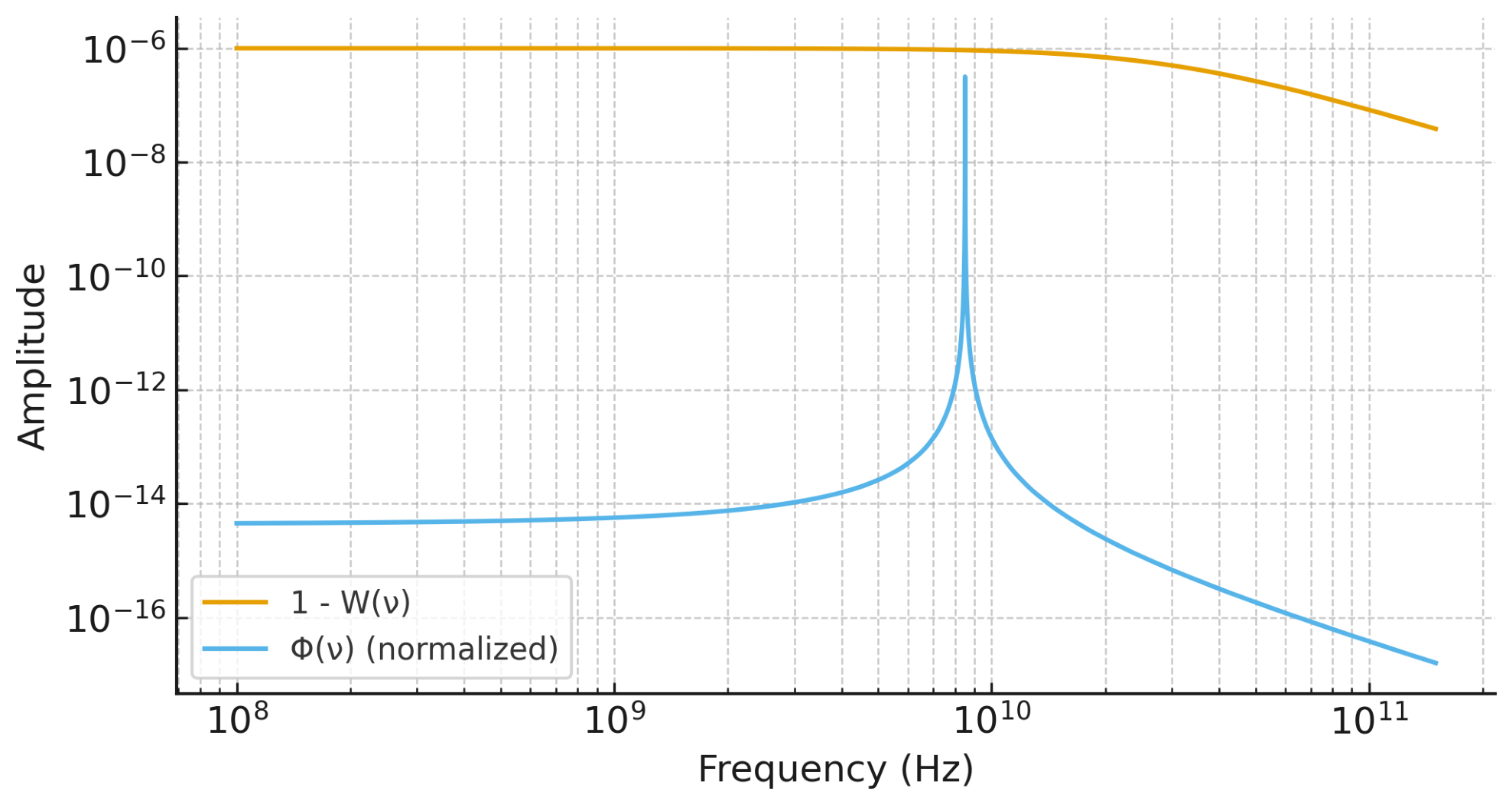
Figure A2.
Causal residual and band window. The broad curve shows and the narrow curve the normalized instrument sensitivity . The curves are shown on a common logarithmic amplitude scale for visual comparison; the numerical integration uses the unit-area normalization of .
Figure A2.
Causal residual and band window. The broad curve shows and the narrow curve the normalized instrument sensitivity . The curves are shown on a common logarithmic amplitude scale for visual comparison; the numerical integration uses the unit-area normalization of .
Appendix B.3. Evaluation of the Band Observable
The band-averaged response is
and the operational quantity is
Because the Lorentzian window is extremely narrow compared with the full plotting interval, Eq. (A25) is evaluated by adaptive quadrature rather than by direct summation over the broadband logarithmic grid.
For numerical stability it is useful to introduce the dimensionless variable
This form resolves the narrow experimental band directly in units of its half-width and avoids requiring an excessively dense frequency grid over the full broadband plotting interval.
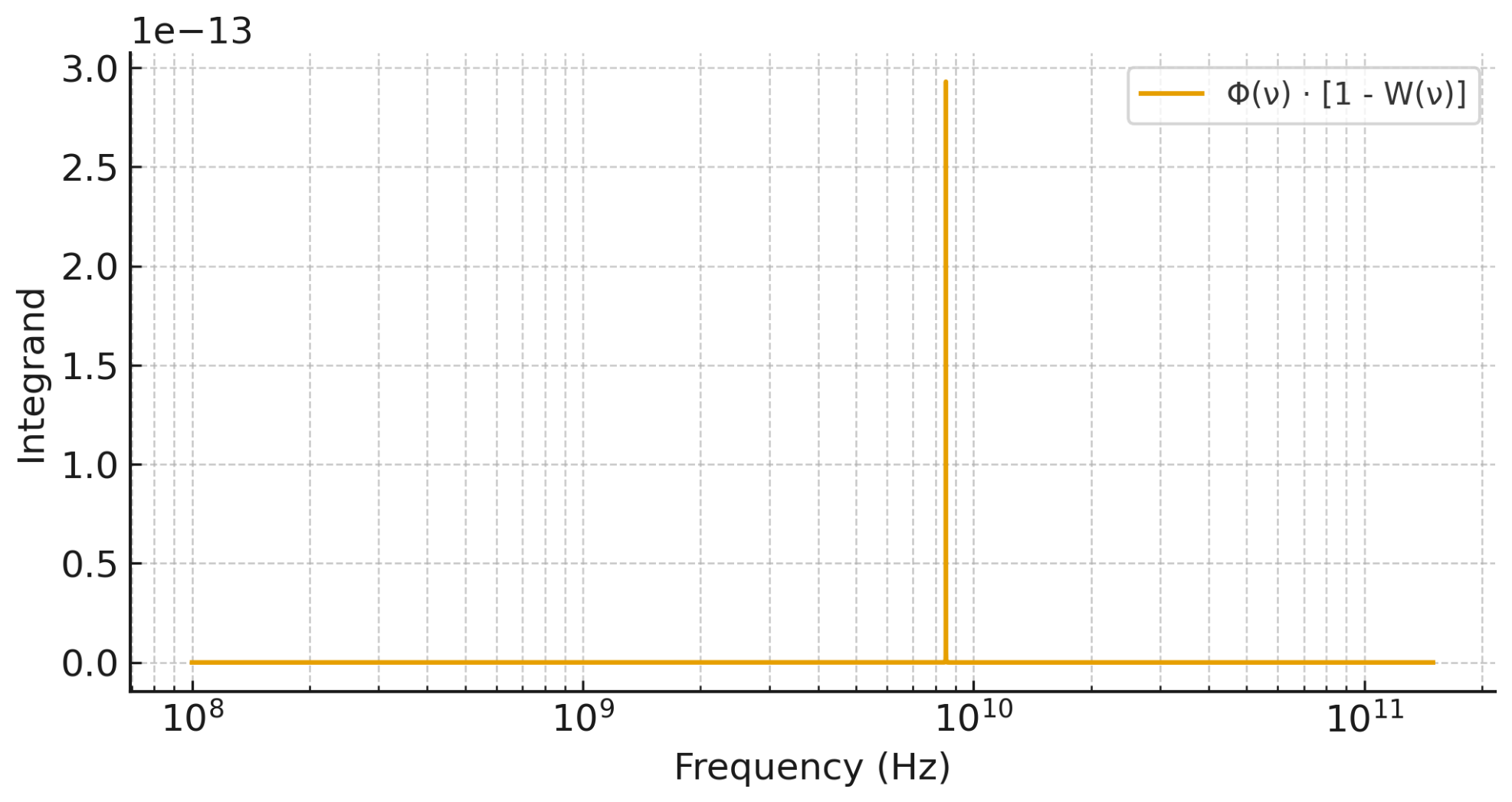
Figure A3.
Integrand for the same parameters as Figure A2. Its integral is , hence .
Figure A3.
Integrand for the same parameters as Figure A2. Its integral is , hence .
Appendix B.4. Parameters of the Worked Example
The numerical parameters are summarized in Table A1.

Table A1.
Parameters used for the numerical worked example. The broadband grid is used for visualization only; the band integral is evaluated by adaptive quadrature using Eq. (A28).
Table A1.
Parameters used for the numerical worked example. The broadband grid is used for visualization only; the band integral is evaluated by adaptive quadrature using Eq. (A28).
| Quantity | Symbol | Value |
|---|---|---|
| Plotting frequency range | – | |
| Broadband plotting points | N | 1000 |
| Band centre | ||
| Lorentzian FWHM | ||
| Lorentzian half-width | ||
| Positive-frequency normalization | ||
| Single-pole amplitude | A | |
| Characteristic frequency | ||
| Weighted response | ||
| Band result |
Appendix B.5. Numerical Procedure and Consistency Checks
The numerical procedure is:
- 1.
- Construct the logarithmic broadband frequency grid used for visualization of the response functions.
- 2.
- Define the positive-frequency Lorentzian and calculate its exact normalization from Eq. (A16).
- 3.
- Form the normalized sensitivity function .
- 4.
- Evaluate the causal response residual from Eq. (A23).
- 5.
- Transform the band integral to the dimensionless variable and evaluate Eq. (A28) using adaptive quadrature.
- 6.
- Resolve the neighbourhood of explicitly, where the narrow sensitivity profile has its maximum, and verify convergence by tightening the numerical tolerance and subdividing the integration interval.
- 7.
- Verify the normalization conditionto the numerical accuracy of the quadrature.
- 8.
-
Verify linearity in the small-response regime by varying the magnitude of A while retaining the passive-response condition . To first order, the magnitude of must scale linearly with A, with the sign fixed by for a positive sensitivity overlap.As an optional code-level consistency check, the calculation may also be repeated formally with to verify algebraic sign reversal. Such a sign-reversed case is used only as a numerical diagnostic: for the single-pole convention adopted here it gives for and therefore lies outside the physically admissible passive-response class.
For the parameters of Table A1, further subdivision of the narrowband integration region and tightening of the adaptive-quadrature tolerance leave the digits reported in Eq. (A31) unchanged.
The numerical example is intended only to demonstrate the operational mapping
It is not used as an experimental constraint and does not determine a microscopic vacuum scale.
Appendix C. Mapping to the Isotropic SME Photon Coefficient
In the minimal photon sector of the Standard-Model Extension (SME), the isotropic CPT-even deformation is conventionally parametrized by the dimensionless coefficient [18,19].
In the standard photon-sector convention of Kostelecký and Mewes, the isotropic electromagnetic constitutive response may be written as
so that the corresponding refractive index is
Within the present phenomenological framework,
and therefore the leading-order correspondence is
when both quantities are interpreted within the same photon-sector reference convention. Consequently,
for an isotropic contribution over the instrument band.
This correspondence is convention dependent. In the full SME, an isotropic photon-sector coefficient can be shifted into matter-sector coefficients by coordinate and field redefinitions. Experimental bounds therefore constrain relative propagation effects with respect to the material rods, clocks, resonators, or particle sectors used as references, rather than an absolute photon-sector quantity in isolation.
Appendix D. Operational Constancy of the Effective Propagation Speed
Appendix D.1. Scope
The purpose of this appendix is limited. We examine how the causal response introduced in the main text can produce an approximately frequency-independent propagation speed over a finite experimental band. We do not attempt to derive the exact SI value of c, Lorentz invariance, or the microscopic electromagnetic constants from vacuum dynamics.
Throughout this appendix,
denotes the dispersive part of the retarded response. In a weakly absorptive band the corresponding phase-propagation speed is
Here c denotes the Maxwell reference speed appearing in the high-frequency limit of the effective theory. Thus is an operational quantity describing departures from that reference within the phenomenological response model.
Appendix D.2. Approximate Constancy within a Measurement Band
For the causal single-pole baseline used in the main text,
with . Its real-frequency dispersive component is
Consequently,
For ,
In the low-frequency regime this becomes
The important point is not that is mathematically exact and frequency independent, but that its variation can be strongly suppressed when the experimental band lies well below the characteristic response scale .
For a finite band , the first-order variation is
Thus an experimentally constant propagation speed over a finite band is compatible with a nontrivial causal response provided that the residual spectral variation lies below the measurement sensitivity. This is the operational sense in which “constancy” is used here.
Appendix D.3. Relation to the Band Observable
The same conclusion can be expressed directly in terms of the band-response quantity . Since , the band-averaged phase-speed shift is, to first order,
A measured value consistent with therefore constrains the band-averaged departure of the effective propagation speed from the Maxwell reference value to the same first-order accuracy.
This statement does not require the response to be constant outside the measured band. It also does not require an assumed ultraviolet shoulder or additional thermodynamic parameters. The relevant information is contained entirely in the causal response and the experimentally specified sensitivity window .
Appendix D.4. Causality, Fluctuations, and What Is Not Derived
The retarded-response framework is compatible with standard fluctuation–dissipation reasoning: in thermal equilibrium, dissipative response and equilibrium fluctuations are related through the fluctuation–dissipation theorem [6,20,21]. In the present framework this supports the requirement that absorption and dispersion must belong to one causal response rather than being specified independently.
The fluctuation–dissipation theorem is not, however, used here to derive , , or the numerical value of c. Such a derivation would require a microscopic theory specifying the relevant vacuum degrees of freedom and their coupling to the electromagnetic field. The operational construction developed in this paper instead asks the more limited question of how a small residual response, if present, could be constrained experimentally.
Likewise, approximate spectral flatness in a given frame does not by itself establish Lorentz invariance. The scalar response used here is specified in the homogeneous and isotropic rest frame of the effective medium. Possible boost-dependent signatures are treated separately in Sec. 4.4. A derivation of observer-independent Lorentz symmetry from microscopic vacuum dynamics lies outside the scope of the present work.
Appendix D.5. Connection with the Low-Energy Expansion
The local low-energy expansion introduced in Section 2.1 separates a constant offset from the frequency-dependent residual:
with
This decomposition is useful when comparing the local effective parametrisation with the global causal single-pole baseline. For
the real-frequency response is
At frequencies ,
The single-pole example therefore contains both ingredients appearing in the general low-energy decomposition: a constant contribution and a quadratic dispersive curvature.
Within this particular response,
The offset-subtracted residual is
This structural similarity does not establish a microscopic identity between the parameters and . Such an identification would require an explicit matching calculation specifying that the two parametrisations arise from the same underlying response.
Operationally, the important distinction is between the constant band contribution and the frequency-dependent curvature. A narrowband measurement may constrain mainly their sum, whereas separated-band, phase–delay, or spectral-slope measurements can in principle isolate the dispersive part.
The low-energy expansion and the causal single-pole model should therefore be regarded as complementary descriptions: the former parametrizes local spectral curvature, while the latter supplies one explicit globally causal and passive response satisfying the Maxwell high-frequency limit.
Appendix D.6. Microscopic Motivation
A possible microscopic motivation for a Maxwell-like low-energy regime is provided schematically by lattice gauge systems. In a deconfined Coulomb phase, a compact -type model can possess gapless transverse modes whose long-wavelength effective description is Maxwell-like.
Higher-dimension operators may then generate corrections suppressed by powers of , motivating an expansion of the type used in Eq. (13).
This observation is included only as a constructive motivation. It does not derive the bounded-vacuum response , determine its parameters, or establish the ultraviolet completion. In particular, the condition as remains an independent admissibility condition on the phenomenological response unless it is obtained from an explicit microscopic theory.
Appendix D.7. Reproducibility of the Operational Quantities
The operational quantities introduced in this work are intended to be independently reproducible. For each experimental application, the calibrated sensitivity window should therefore be made available in machine-readable form together with the numerical procedure used to evaluate
Where a result is derived from measured transfer functions or composite calibration products, the corresponding processing scripts, frequency grid, normalization convention, uncertainty treatment, and versioned input data should also be archived.
Providing both and the reported value of allows the result to be re-integrated for alternative admissible response functions without reconstructing the original apparatus model. This is particularly important for cross-platform comparison, because the instrument-specific information remains contained in while the vacuum-response hypothesis can be varied independently. Data and analysis code should, where possible, be deposited in a persistent repository with a DOI, in accordance with established reproducible-research practice [30,31,35,38].
Appendix D.8. Summary
Within the present model, the experimentally relevant claim is therefore modest: a causal response can differ slightly from unity while producing a propagation speed that is effectively constant over a finite measurement band. The magnitude and spectral variation of that departure are directly testable through . No claim is made in this appendix that the observed value of c, Lorentz symmetry, or the electromagnetic constants have already been derived from bounded-vacuum dynamics.
Appendix E. First-Order Lifshitz Variation for an Impedance-Invariant Gap Response
The purpose of this appendix is to connect the operational vacuum response to Casimir-type observables without assuming that the unrenormalized zero-point energy is finite. The relevant quantity is the change in the renormalized Lifshitz interaction produced by a small deformation of the electromagnetic response in the gap.
Throughout this appendix we work on the imaginary-frequency axis and define
For the passive causal responses considered here, is real on the positive imaginary axis. We write
The subscript E is used only to emphasize that this is the analytic continuation of the retarded response to imaginary frequency; it is not an independent response function.
Appendix E.1. Lifshitz Interaction in a Modified Gap
For two parallel planar bodies separated by a distance a, the zero-temperature Lifshitz interaction energy per unit area can be written as [4,17,25,29]
where
is the product of the two polarization-dependent reflection coefficients.
The electromagnetic response in the gap is described by the relative constitutive functions
The equal co-scaling preserves the gap impedance while modifying its propagation constant. The imaginary-frequency wave number in the gap is therefore
For the Maxwell reference state ,
The material response functions of the plates are treated as externally specified calibration inputs. Nevertheless, the Fresnel coefficients can still depend on the gap response through the boundary matching conditions and therefore need not remain fixed when is varied.
Appendix E.2. First-Order Variation of the Gap Propagation Factor
The derivative of Eq. (A61) with respect to is
Consequently, expanding around the Maxwell reference state gives
to first order. This factor is important: in general, . The transverse wave number therefore remains explicitly present in the sensitivity of the Lifshitz kernel to the vacuum response.
Appendix E.3. Variation of the Lifshitz Energy
Define
For a small variation,
with
Hence, evaluated at the Maxwell reference state,
Using Eq. (A64), the contribution arising directly from propagation through the modified gap is therefore
The second term in Eq. (A68) represents the change of the boundary reflection amplitudes. Explicitly,
These terms should not in general be set to zero. Even when the gap impedance itself is unchanged by the co-scaling , the gap propagation constant entering the Fresnel boundary problem changes. A complete material calculation must therefore either evaluate explicitly or absorb the resulting boundary sensitivity into the experimentally calibrated Casimir response kernel.
Appendix E.4. Force Variation and Casimir Sensitivity Kernel
The Casimir force per unit area is
The complete first-order response can therefore be written formally as a linear functional of the imaginary-frequency deformation,
where contains both the explicit propagation contribution generated by Eq. (A64) and any first-order change of the TE/TM reflection amplitudes associated with the modified gap response.
The detailed form of depends on plate materials, separation, temperature, polarization, geometry, and the chosen calibration model. It is therefore an instrument-specific response kernel rather than a universal function. Importantly, need not be positive at every frequency. Casimir measurements therefore provide a natural example of the more general signed-kernel formulation discussed in Section 1.
If
is nonzero, one may define the normalized kernel
Equation (A72) then becomes
Defining, in analogy with the real-frequency band observable,
gives
to first order. Thus the band quantity remains a convenient measure of the spectral deformation, but the conversion to an observed fractional force shift contains the platform-dependent sensitivity factor . Only in a convention where this sensitivity has already been absorbed into the response kernel does the proportionality coefficient become unity.
Appendix E.5. Finite Temperature
At nonzero temperature, the continuous imaginary-frequency integral is replaced by the standard Matsubara sum,
The same first-order construction applies term by term: the gap propagation factor, reflection amplitudes, and corresponding sensitivity kernel are evaluated at the Matsubara frequencies. No new assumption about the vacuum response is required.
Appendix E.6. Ultraviolet Behaviour
The Casimir consistency condition used throughout this work is
This condition does not regularize the unrenormalized zero-point energy. Rather, it ensures that the proposed deformation becomes asymptotically negligible and that the standard electromagnetic ultraviolet structure of the Lifshitz problem is recovered. The resulting observable is the change in the renormalized interaction, not a bare vacuum-energy integral. This is the restricted meaning of Casimir-safe adopted in this paper.
Appendix E.7. Scope
Appendix E establishes only the first-order functional connection between a small imaginary-frequency deformation of the vacuum response and a Casimir observable. It does not claim that existing Casimir data already determine uniquely.
A quantitative constraint requires the actual experimental geometry, material response functions, temperature, plate separation, calibration model, and uncertainty budget. Once these are specified, the resulting or normalized can be published and used to constrain admissible forms of in the same reproducible spirit as the real-frequency response windows considered elsewhere in this work.
Appendix F. Conceptual Outlook and Open Conjectures
Scope and status.
The operational results of this paper require only the retarded, frequency-dependent response introduced in the main text. The present appendix discusses possible extensions beyond that framework. These remarks are explicitly conjectural: they are not used in deriving , do not constitute a microscopic theory of the vacuum, and are not claimed as consequences of the measurements considered here.
Frequency response versus covariant form factors.
A response describes dispersion with respect to the frequency measured in the homogeneous and isotropic frame in which the response is specified. A formally Lorentz-covariant nonlocal extension may instead involve an operator-valued form factor, for example
The two constructions are not automatically equivalent. In particular, a function of □ alone does not, by simple substitution, reproduce an arbitrary refractive response . A microscopic derivation may require additional dynamical structure, such as interactions, a preferred macroscopic four-velocity, curvature dependence, or a more general causal nonlocal kernel. Establishing such a derivation lies outside the scope of the present work.
Consequently, this paper does not claim to derive Lorentz symmetry from the flatness of W, nor does it claim that Lorentz covariance and a frequency-dependent vacuum index have already been unified. The experimentally relevant statement is more limited: within the operational regime, sufficiently small and smooth deviations from can be constrained through while causality and the Maxwell high-frequency limit are imposed as admissibility conditions.
Possible cross-sector generalisation.
It is natural to ask whether analogous response functions could be defined for other field sectors. A conservative research programme would test, rather than assume, the following possibilities:
- 1.
- sector-dependent response functions may obey common analyticity, positivity or passivity constraints;
- 2.
- their ultraviolet limits may approach the corresponding standard field theories;
- 3.
- a common dynamical origin for such constraints may exist.
These possibilities amount to hypotheses for future model building. They do not by themselves establish unification of electromagnetic, weak, strong, or gravitational interactions.
Stability as an open dynamical question.
Analyticity, passivity and ultraviolet normalisation define an admissible class of responses, but admissibility alone does not prove dynamical attraction toward . A genuine stability or fixed-point claim would require an explicit evolution or renormalisation equation, schematically
together with a specified state space, fixed points of , and a linear or nonlinear stability analysis. No such dynamics is assumed in the present paper. Accordingly, terms such as “self-correction”, “attractor”, or “emergent physical law” should be understood only as motivations for future work until such a dynamical construction is supplied.
As illustrated schematically in Figure A4, the admissibility conditions used in this work constrain the allowed response class but do not define a dynamical evolution toward that class.
Figure A4.
Conceptual schematic of admissibility versus open dynamics. Analyticity, passivity, and ultraviolet normalization define an admissible class of causal vacuum-response functions , but do not by themselves establish dynamical attraction, self-correction, or fixed-point behaviour. Any such stability claim would require an explicit evolution or renormalization law together with a specified state space and a corresponding stability analysis.
Figure A4.
Conceptual schematic of admissibility versus open dynamics. Analyticity, passivity, and ultraviolet normalization define an admissible class of causal vacuum-response functions , but do not by themselves establish dynamical attraction, self-correction, or fixed-point behaviour. Any such stability claim would require an explicit evolution or renormalization law together with a specified state space and a corresponding stability analysis.
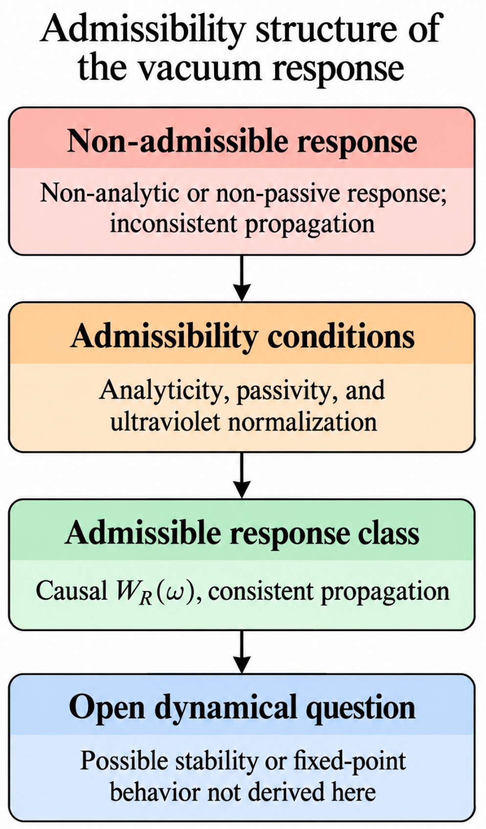
Outlook.
The useful conceptual question raised by the present framework is therefore narrower than a claim of unification: can the same physically admissible response structure that makes the photonic vacuum operational also arise from a microscopic theory, and can analogous structures be identified independently in other sectors? The current paper provides the photonic observable as a falsifiable interface for the first part of that programme. Any broader emergence or unification claim remains conditional on additional dynamics and independent tests.
Appendix G. SME-Conditioned Experimental Recast of a Precision Optical-Resonator Constraint
Appendix G.1. Purpose and Scope
The operational framework developed in this work is intended to connect a hypothetical vacuum response to quantities constrained by precision experiments. The numerical example in Appendix B demonstrates the integration procedure for a prescribed response and instrument window, but it does not itself provide an experimental constraint.
In this appendix we therefore apply the framework to a published laboratory result. We use the odd-parity asymmetric optical-resonator experiment of Baynes, Luiten, and Tobar [2], which reported a laboratory constraint on the isotropic photon-sector Standard-Model Extension coefficient . The present analysis is an SME-conditioned experimental recast rather than an independent reanalysis of the experimental time series. No new experimental data are introduced, and the original SME signal model is not refitted. Instead, the published constraint is translated into the operational vacuum-response quantity using the correspondence developed in Section 4.1.
The translation is conditional on identifying the approximately frequency-independent isotropic component of the phenomenological response with the isotropic minimal-SME photon-sector coefficient, under the corresponding SME reference-sector and transformation assumptions [18,19]. It therefore does not establish that an arbitrary vacuum-response model is subject to the same numerical constraint without further specification of its transformation law and matter-sector reference conventions.
Appendix G.2. Published Optical-Resonator Constraint
Baynes, Luiten, and Tobar used an asymmetric odd-parity optical ring resonator and compared the frequencies of counter-propagating fundamental modes [2]. The asymmetry of the resonator provides sensitivity to Lorentz-violating photon-sector coefficients that is complementary to conventional even-parity resonator configurations.
The experiment reported
where the quoted uncertainty corresponds to one standard deviation () [2]. The measured value is statistically compatible with zero and therefore constitutes a constraint rather than evidence for a nonzero isotropic propagation anomaly.
For comparison, an earlier analysis by Hohensee et al. using rotating cryogenic sapphire oscillators constrained with a precision of approximately [12]. The optical odd-parity result of Baynes et al. therefore provides a useful laboratory benchmark for the present recast.
Appendix G.3. Mapping to the Vacuum-Response Observable
As discussed in Section 4.1, conditional on the common photon-sector reference convention and the corresponding minimal-SME transformation assumptions, the leading-order comparison is
The operational band quantity is
For a response that is effectively frequency independent over the experimental optical bandwidth,
the normalization of the sensitivity function gives
Using Eq. (A83), one obtains
The published Baynes et al. result can therefore be expressed, under the stated SME-conditioned correspondence, as
Equation (A88) should be understood as an experimentally anchored recast of the published SME result into the band-response quantity . It is not an independent measurement of .
Appendix G.4. Conservative Upper Limit
For illustration, if the uncertainty in Eq. (A82) is treated as Gaussian, an approximate two-sided confidence interval is
corresponding approximately to
This confidence-level conversion is performed here only to express the published result as a simple operational upper envelope. It does not replace the statistical analysis performed in the original experiment.
Appendix G.5. Implication for an Approximately Constant Vacuum Response
For an admissible response that is sufficiently flat across the experimental sensitivity band,
Eq. (A92) implies, conditional on the SME mapping,
Within the present phenomenological parametrization,
so that, to first order,
The corresponding operational envelope is therefore
for the isotropic, effectively frequency-independent component under the experimental, reference-sector, and transformation assumptions associated with the SME recast.
This expression must not be interpreted as an absolute measurement of the speed of light independent of matter-sector standards. In the SME comparison, experimental constraints apply to relative propagation effects with respect to the material rods, clocks, resonators, or particle sectors defining the measurement reference [18,19].
Appendix G.6. Relation to the Causal Single-Pole Response
The causal baseline used elsewhere in this work is
with real-frequency dispersive component
For a normalized experimental sensitivity function , the corresponding band observable is
It is convenient to define the overlap factor
Then
If an experiment provides an upper limit
then, provided that
the response amplitude satisfies
The absolute value in Eq. (A105) is required for the general case because an experimentally calibrated sensitivity kernel need not be positive at every frequency. For the positive normalized kernels used in the simple worked examples, , and the expression reduces to the corresponding form without the absolute value.
If , the experimental weighting is orthogonal, at first order, to the single-pole response shape at that value of . The experiment then has vanishing first-order sensitivity to the amplitude A, and no constraint on A can be inferred from at this order.
For the SME-conditioned recast derived above, the approximate Gaussian envelope corresponds to
Substitution into Eq. (A105) therefore gives the formal exclusion relation
subject to the SME identification, reference-sector convention, and transformation assumptions specified in the preceding subsections.
A numerical exclusion curve cannot, however, be obtained from the published SME coefficient alone. It requires the actual calibrated spectral sensitivity function , or a sufficiently justified reconstruction of that function, so that can be evaluated across the relevant range of . Accordingly, Eq. (A105) should be regarded as the experimentally anchored constraint relation for the causal single-pole model, while no numerical frequency-dependent exclusion curve is claimed here without additional instrument-response information.
Appendix G.7. Relation to the Quadratic Low-Energy Parametrisation
The quadratic low-energy parametrisation introduced in Section 2.1 applies to the offset-subtracted dispersive component,
The corresponding dispersive band observable is
which gives, to leading order,
where
If an experiment provides a calibrated upper limit
then
The SME-conditioned envelope derived in the preceding subsections,
constrains an approximately frequency-independent isotropic response under the corresponding SME reference-sector and transformation assumptions. It should therefore not be identified automatically with .
In particular, the published value of alone does not determine the sensitivity of the experiment to the quadratic spectral curvature in Eq. (A108). Such an interpretation requires the calibrated spectral sensitivity function , together with the appropriate signal model and transformation law, so that the constant and frequency-dependent components can be separated.
Consequently, no numerical value of is inferred here from the published SME coefficient alone. Once a calibrated constraint on is available, however, Eq. (A113) provides the corresponding model-dependent lower bound on the effective dispersive scale.
This relation is not an SME bound and does not determine a microscopic vacuum scale. It is the consequence of applying an experimentally determined dispersive band constraint to the specific quadratic low-energy parametrisation of the present response framework.
Appendix G.8. Interpretation and Limitations
The result of this appendix should be interpreted at three distinct levels. First, the experimentally reported quantity
is taken from the optical-resonator experiment of Baynes, Luiten, and Tobar [2]. Second, the relation
is the operational recast introduced in the present work. It applies to an effectively frequency-independent isotropic response across the experimental band, conditional on the common photon-sector reference convention and the corresponding SME transformation assumptions. Third, the approximate bound
is a derived Gaussian confidence-envelope estimate based on the published central value and quoted uncertainty. It is not a new fit to the original experimental data.
The recast therefore provides an experimentally anchored constraint on the constant or sufficiently slowly varying component of the operational vacuum response, conditional on its identification with the isotropic minimal-SME photon-sector coefficient and on the associated reference-sector and transformation assumptions. It does not provide a model-independent constraint on an arbitrary frequency-dependent response . Such a constraint would require the calibrated sensitivity function , its uncertainty, and a specified transformation law for the response. With that information, Eqs. (A105) and the quadratic bound above could be evaluated directly for particular causal response models.
Appendix G.9. Summary
The principal experimentally anchored translation obtained in this appendix is
at the reported level, together with the approximate Gaussian envelope
This result does not constitute a new measurement, a new fit to the original experimental data, or a detection of a nontrivial vacuum response. It demonstrates that, under the stated SME identification, reference-sector convention, and transformation assumptions, the operational quantity can be connected quantitatively to an existing precision-photonic laboratory constraint.
The conditional logical chain is therefore
References
- Aspelmeyer, M.; Kippenberg, T. J.; Marquardt, F. Cavity optomechanics. Rev. Mod. Phys. 2014, 86, 1391–1452. [Google Scholar] [CrossRef]
- Baynes, F. N.; Luiten, A. N.; Tobar, M. E. Testing Lorentz invariance using an odd-parity asymmetric optical resonator. Phys. Rev. D. 2011, 84, 081101(R). [Google Scholar] [CrossRef]
- Bimonte, G.; López, D.; Decca, R. S. Isoelectronic determination of the thermal Casimir force. Phys. Rev. B 2016, 93, 184434. [Google Scholar] [CrossRef]
- Bordag, M.; Klimchitskaya, G. L.; Mohideen, U.; Mostepanenko, V. M. Advances in the Casimir Effect; Oxford University Press, 2009; ISBN 978-0199238743. [Google Scholar]
- Carr, S. M.; Woods, S. I.; Jung, T. M.; Carter, A. C.; Datla, R. U. Experimental measurements and noise analysis of a cryogenic radiometer. Rev. Sci. Instrum. 2014, 85, 075105. [Google Scholar] [CrossRef] [PubMed]
- Callen, H. B.; Welton, T. A. Irreversibility and Generalized Noise. Phys. Rev. 1951, 83, 34–40. [Google Scholar] [CrossRef]
- Calloni, E.; Di Fiore, L.; Esposito, G.; Rosa, L. Gravitational experiments in a quantum vacuum. Phys. Rev. D. 2015, 91, 102002. [Google Scholar] [CrossRef]
- Casimir, H. B. G. On the attraction between two perfectly conducting plates. Proc. K. Ned. Akad. Wet. 1948, 51, 793. [Google Scholar]
- Creedon, D. L.; Reshitnyk, Y.; Farr, W. G.; Martinis, J. M.; Duty, T. L.; Tobar, M. E. High Q-factor sapphire whispering gallery mode microwave resonator at single photon energies and millikelvin temperatures. Appl. Phys. Lett. 2011, 98, 222903. [Google Scholar] [CrossRef]
- Decca, R. S.; López, D.; Fischbach, E.; Krause, D. E. Measurement of the Casimir force between dissimilar metals. Phys. Rev. Lett. 2005, 94, 240401. [Google Scholar] [CrossRef]
- Fixsen, D. J. The Temperature of the Cosmic Microwave Background. Astrophys. J. 2009, 707, 916–920. [Google Scholar] [CrossRef]
- Hohensee, M. A.; Stanwix, P. L.; Tobar, M. E.; Parker, S. R.; Phillips, D. F.; Walsworth, R. L. Improved constraints on isotropic shift and anisotropies of the speed of light using rotating cryogenic sapphire oscillators. Phys. Rev. D. 2010, 82, 076001. [Google Scholar] [CrossRef]
- Jackson, J. D. Classical Electrodynamics, 3rd ed.; Wiley, 1999. [Google Scholar]
- Jaffe, R. L. The Casimir effect and the quantum vacuum. Phys. Rev. D. 2005, 72, 021301(R). [Google Scholar] [CrossRef]
- Kamminga, A. J. H. Vacuum Density and Cosmic Expansion: A QEV Model. Preprints 2025. [Google Scholar] [CrossRef]
- Kamminga, A. J. H. Vacuum Energy with Natural Bounds: A Spectral Approach without Fine-Tuning. Preprints 2025. [Google Scholar] [CrossRef]
- Klimchitskaya, G. L.; Mohideen, U.; Mostepanenko, V. M. The Casimir force between real materials: Experiment and theory. Rev. Mod. Phys. 2009, 81, 1827–1885. [Google Scholar] [CrossRef]
- Kostelecký, V. A.; Mewes, M. Signals for Lorentz Violation in Electrodynamics. Phys. Rev. D. 2002, 66, 056005. [Google Scholar] [CrossRef]
- Kostelecký, V. A.; Russell, N. Data Tables for Lorentz and CPT Violation. Rev. Mod. Phys. 2011, 83, 11–31. [Google Scholar] [CrossRef]
- Kubo, R. Statistical-Mechanical Theory of Irreversible Processes. J. Phys. Soc. Jpn. 1957, 12, 570. [Google Scholar] [CrossRef]
- Kubo, R. The fluctuation-dissipation theorem. Rep. Prog. Phys. 1966, 29, 255–284. [Google Scholar] [CrossRef]
- Landau, L. D.; Lifshitz, E. M. Electrodynamics of Continuous Media, 2nd ed.; Pergamon, Oxford, 1984. [Google Scholar]
- Lamoreaux, S. K. Demonstration of the Casimir Force in the 0.6 to 6 μm Range. Phys. Rev. Lett. 1997, 78, 5–8. [Google Scholar] [CrossRef]
- Mather, J. C.; Fixsen, D. J.; Shafer, R. A.; Mosier, C.; Wilkinson, D. T. Calibrator design for the COBE Far Infrared Absolute Spectrophotometer (FIRAS). Astrophys. J. 1999, 512, 511–520. [Google Scholar] [CrossRef] [PubMed]
- K. A. Milton, The Casimir Effect: Physical Manifestations of Zero-Point Energy; World Scientific, 2001.
- Milton, K. A. The Casimir effect: Recent controversies and progress. J. Phys. A Math. Gen. 2004, 37, R209–R277. [Google Scholar] [CrossRef]
- Milton, K. A. Applications of the Casimir effect. J. Phys. Conf. Ser. 2011, 161, 012001. [Google Scholar] [CrossRef]
- Mohideen, U.; Roy, A. Precision Measurement of the Casimir Force from 0.1 to 0.9 μm. Phys. Rev. Lett. 1998, 81, 4549–4552. [Google Scholar] [CrossRef]
- Mostepanenko, V. M. Status of modern Casimir force measurements and theoretical approaches. Universe 2021, 7, 84. [Google Scholar] [CrossRef]
- Nosek, B. A.; et al. Promoting an open research culture. Science 2015, 348, 1422–1425. [Google Scholar] [CrossRef] [PubMed]
- Peng, R. D. Reproducible research in computational science. Science 2011, 334, 1226–1227. [Google Scholar] [CrossRef] [PubMed]
- Planck Collaboration, Planck 2018 results. I. Overview and the cosmological legacy of Planck. Astron. Astrophys. 2020, 641, A1. [CrossRef]
- Kaplan, S. G.; Woods, S. I.; Shirley, E. L.; Carter, A. C.; Jung, T. M.; Proctor, J. E.; Sears, D. R.; Zeng, J. Design, calibration, and application of a cryogenic low-background infrared radiometer for spectral irradiance and radiance measurements from 4 to 20 μm wavelength. Opt. Eng. 2021, 60(3), 034102. [Google Scholar] [CrossRef] [PubMed]
- Pate, J. M.; Goryachev, M.; Chiao, R. Y.; Sharping, J. E.; Tobar, M. E. Casimir spring and dilution in macroscopic cavity optomechanics. Nat. Phys. 2020, 16, 1117–1122. [Google Scholar] [CrossRef]
- Stodden, V.; McNutt, M.; Bailey, D. H.; et al. Enhancing reproducibility for computational methods. Science 2016, 354, 1240–1241. [Google Scholar] [CrossRef] [PubMed]
- Urban, M.; Couchot, F.; Sarazin, X.; Djannati-Atai, A. The quantum vacuum as the origin of the speed of light. Eur. Phys. J. D. 67 2013, 58. [Google Scholar] [CrossRef]
- Wiens, E.; Kwong, C. J.; Müller, T.; Schiller, S. A simplified cryogenic optical resonator apparatus providing ultra-low frequency drift. Rev. Sci. Instrum. 2020, 91, 045112. [Google Scholar] [CrossRef] [PubMed]
- Wilson, G.; Bryan, J.; Cranston, K.; Kitzes, J.; Nederbragt, L.; Teal, T. K. Good enough practices in scientific computing. PLoS Comput. Biol. 2017, 13, e1005510. [Google Scholar] [CrossRef] [PubMed]
Figure 1.
Operational pipeline: a single vacuum window and a calibrated, unit-area sensitivity combine into the common cross-platform reporting quantity . Normalization: . Schematic, not to scale.
Figure 1.
Operational pipeline: a single vacuum window and a calibrated, unit-area sensitivity combine into the common cross-platform reporting quantity . Normalization: . Schematic, not to scale.

Disclaimer/Publisher’s Note: The statements, opinions and data contained in all publications are solely those of the individual author(s) and contributor(s) and not of MDPI and/or the editor(s). MDPI and/or the editor(s) disclaim responsibility for any injury to people or property resulting from any ideas, methods, instructions or products referred to in the content. |
© 2026 by the authors. Licensee MDPI, Basel, Switzerland. This article is an open access article distributed under the terms and conditions of the Creative Commons Attribution (CC BY) license (http://creativecommons.org/licenses/by/4.0/).
Copyright: This open access article is published under a Creative Commons CC BY 4.0 license, which permit the free download, distribution, and reuse, provided that the author and preprint are cited in any reuse.