Submitted:
03 November 2025
Posted:
05 November 2025
You are already at the latest version
Abstract
This study explores the role of Decentralized Physical Infrastructure Networks (DePIN) in enhancing solar energy forecasting, focusing on the effects of network density on prediction accuracy and economic viability. Utilizing machine learning models applied to distributed solar power data from 47 residential PV systems in Utrecht, Netherlands, we develop a hierarchical forecasting framework: Level 1 (clear-sky baseline without historical data), Level 2 (solo forecasting with local historical data), and Level 3 (networked forecasting incorporating neighboring installations). Results indicate that increasing network density significantly improves forecasting accuracy, with the most substantial gains occurring when integrating data from the first 10-15 neighbors, reducing Mean Absolute Error (MAE) by up to 17% compared to solo approaches. Ensemble methods like Random Forest and XGBoost demonstrate superior performance in leveraging spatial correlations. Economically, these accuracy improvements translate to imbalance cost reductions of up to 27% relative to non-data-driven baselines, based on Dutch market data. Marginal benefit analysis reveals diminishing returns beyond local clustering (5-10 km radii), providing a foundation for incentive mechanisms in DePIN ecosystems. By addressing data fragmentation through privacy-preserving sharing, DePIN fosters cost savings for energy traders and revenue opportunities for participants, advancing decentralized energy markets.
Keywords:
DePIN
; solar energy
; machine learning
; forecasting
; network density
; economic impact
; data silos
1. Introduction
The global transition toward renewable energy sources has accelerated in recent years, driven by the urgent need to mitigate climate change and enhance energy security [1,2]. Among various renewable options, solar power has emerged as a particularly attractive choice due to its declining costs, scalability, and widespread resource availability [3]. Nevertheless, the integration of solar power into conventional grids presents significant challenges related to its inherent variability and intermittency. Fluctuations in solar irradiance due to weather conditions, seasonal patterns, and diurnal cycles can introduce substantial uncertainty into power generation [4,5].
Accurate forecasting of solar power output is crucial for minimizing the economic and technical issues associated with this variability. When forecasts are inaccurate, energy providers often face imbalance costs, as they must rely on expensive backup power or balancing services to meet contractual obligations [6]. This challenge becomes more pressing as the share of solar power in the energy mix grows, increasing the grid’s vulnerability to forecast errors [7,8].
Despite widespread smart meter deployment, operational PV data remain fragmented across balance groups: BRPs do not routinely access meter-level production from other BRPs’ portfolios due to confidentiality, competition, and governance constraints embedded in current market roles and data-access regimes [9,10,11,12,13]. Public EU data services focus on aggregated market information rather than cross-party, meter-level operational streams needed for localized spatio-temporal PV nowcasting (e.g., the ENTSO-E Transparency Platform) [14].
A promising solution to address data fragmentation and improve solar forecasting accuracy lies in Decentralized Physical Infrastructure Networks (DePIN), which offer a fundamentally different, user-driven approach to decentralized data collection [15]. Rather than relying on top-down systemic changes or limited regional data sources, DePIN empowers individual photovoltaic (PV) owners—prosumers—to voluntarily share localized production data via tokenized incentive mechanisms and blockchain-based platforms [16,17,18,19,20,21]. This creates a bottom-up, privacy-preserving data commons that bypasses traditional institutional barriers [20,22,23], generating cross-balance-group operational streams needed for accurate nowcasting while maintaining commercial confidentiality. By fostering a dense, geographically distributed array of solar nodes, DePIN provides granular insights into fluctuating weather conditions and real-time nowcasting, thereby enhancing prediction models with advanced machine learning integration [5,24]. This facilitates direct participation in peer-to-peer data and energy markets, with automated mechanisms incentivizing contributors, unlocking novel economic opportunities in the solar sector, and aligning with evolving EU data-sharing frameworks [9,10].
Moreover, although decentralized energy systems have garnered attention for facilitating peer-to-peer trading and grid flexibility, the existing literature often examines market design, transaction mechanisms, or blockchain frameworks without systematically quantifying the direct relationship between network density, forecast accuracy, and economic returns [20]. Consequently, there is a pressing need for an integrated study that links these three components—network density, solar forecasting accuracy, and financial viability—within a Decentralized Physical Infrastructure Network (DePIN) setting.
This study addresses two interconnected questions:
- Technical impact: How does increasing network density improve the accuracy of solar power forecasts?
- Economic impact: What financial benefits accrue to energy traders and DePIN participants from these accuracy gains?
We provide three key advancements:
- Network Density vs. Forecast Accuracy Model: A machine learning model quantifying how node density improves prediction accuracy, validated across multiple geographies.
- Cost-Saving Analysis: We quantify how improvements in forecasting reduce imbalance costs.
- DePIN Profitability Model: A revenue projection model that evaluates DePIN user’s returns for sharing data
By bridging the technical and economic dimensions of solar forecasting, our study provides valuable insights into how dense, decentralized sensor networks can facilitate more accurate prediction, reduce operational costs, and create new revenue streams in emerging energy markets.
The remainder of this paper is organized as follows: Section 2 reviews relevant literature on solar forecasting methods, the DePIN paradigm, and the economic implications of accurate predictions. Section 3 outlines our dataset, forecasting methodology, and the economic model for DePIN profitability. Section 4 presents the results, highlighting improvements in forecast accuracy and associated cost savings. Section 5 discusses key findings and practical implications, followed by Section 6, which concludes with a summary of contributions and future research directions.
2. Literature Review
2.1. Solar Forecasting Methods and Networked Systems
Solar photovoltaic (PV) power forecasting has attracted significant interest due to the increasing penetration of solar energy into modern grids [1,3]. Accurate forecasts help mitigate imbalance costs associated with the variability of solar irradiance [6,7]. Over the past decade, research in this field has produced a broad range of methods, typically grouped into three categories:
- Physical approaches: These rely on numerical weather prediction (NWP) or satellite imagery to estimate irradiance, subsequently converting this irradiance to expected PV output using device-specific models. While such methods provide physically interpretable forecasts, their accuracy can be limited by coarse weather model resolutions and uncertainty in module characteristics [7,8].
- Statistical approaches: Approaches such as ARIMA, SARIMA, regression-based models, or time-series decomposition exploit historical data to capture seasonality, trends, and temporal correlations [25]. They often require fewer input variables but may struggle with rapid changes in irradiance or small-scale, localized weather phenomena.
- Machine learning and deep learning methods: Artificial Neural Networks (ANNs), Support Vector Machines (SVMs), Random Forests, and more recently Long Short-Term Memory (LSTM) and other deep neural network architectures, have demonstrated strong performance by uncovering nonlinear, high-dimensional relationships in the data [26,27,28]. Various hybrid or ensemble methods, combining physical and data-driven models, can further improve accuracy by leveraging both domain knowledge and large-scale training datasets [29].
A comprehensive overview of these forecasting techniques is provided by Mellit et al. [24], who discuss the evolution from simple statistical or stand-alone machine learning models to more sophisticated hybrid and deep learning approaches. Despite this extensive body of work, the literature tends to focus on single-site or small-scale network forecasts. Few studies explicitly evaluate how network density (the number of distributed PV nodes sharing real-time measurements over a given geographical area) impacts forecasting performance.
Traditionally, PV output forecasting has relied on single-site models that use data from one or a small number of installations to predict local irradiance and power output [7]. Although such approaches benefit from simplicity and lower data management requirements, they often fall short of capturing the spatial heterogeneity induced by local weather dynamics, cloud cover variability, and other site-specific factors. In contrast, a networked approach aggregates data from multiple, geographically dispersed PV systems, thereby leveraging spatial correlations to enhance forecasting performance. Dense sensor networks offer enhanced spatial resolution by capturing fine-scale fluctuations in solar irradiance due to transient cloud movements and microclimatic effects, as demonstrated by Graabak et al. [30] and Droste et al. [31]. Moreover, by smoothing out local anomalies and measurement errors, distributed data improves forecast robustness, with studies such as Hintz et al. [32] reporting a reduction in output variability. Networked approaches also enable advanced models—such as spatio-temporal graph neural networks—to better capture spatial dependencies among PV systems, which yields significantly improved short-term forecasts as evidenced by Simeunovic et al. [33] and Jang et al. [28]. Recent advances in artificial intelligence have further refined these methods: Mellit et al. [24] provide a comprehensive review of AI techniques that exploit multi-site data for multistep-ahead predictions, while dynamic physical models like PVPro [34] extract system parameters from recent production data to more accurately convert irradiance into power output, even with limited historical data. Hybrid approaches that combine statistical methods (e.g., SARIMA) with machine learning models such as SVMs also underline the advantage of using dense, networked datasets to capture nonlinear system behavior [29].
Overall, transitioning from single-site to networked forecasting frameworks promises significant improvements in accuracy and reliability, ultimately facilitating better grid integration and energy management for distributed PV systems.
2.2. Network Density and Forecasting Accuracy: Insights from Cross-Domain Applications
The relationship between sensor density and forecasting accuracy has been validated across multiple domains.
In meteorology, increasing the density of observations can markedly enhance forecast accuracy by capturing fine-scale spatial and temporal variability. For example, [31] demonstrated that urban air temperature retrievals in São Paulo improve significantly when more than 700 smartphone battery temperature readings are available within a local area. Likewise, [35] showed that crowdsourced temperature data from citizen weather stations in Berlin capture urban heat island effects with far greater spatial detail than traditional networks. Moreover, [32] found that quality-controlled smartphone pressure observations (despite inherent noise) can be effectively assimilated into numerical weather prediction models to improve analyses of surface pressure and wind, even though challenges remain for temperature forecasts [36].
In transportation forecasting, the density of sensory data plays a crucial role in improving prediction accuracy. For instance, [37] demonstrate that an optimally deployed sensor network—one that carefully selects a subset of sensors to ensure full network observability—enables more accurate reconstruction of traffic flows and associated pollutant emissions. In the context of smart cities, [38] highlights that the integration of IoT devices can create high-density sensor networks that enhance real-time data collection, leading to more effective traffic management and forecasting. Meanwhile, [39] show that deep learning models such as Long Short-Term Neural Networks benefit from richer, more frequent data inputs; higher sensor density allows these models to better capture the nonlinear dynamics of traffic speeds, improving both accuracy and stability in predictions. Similarly, [40] demonstrates that using a deep architecture built with stacked autoencoders, the abundance of sensor data helps uncover complex spatial and temporal correlations in traffic flow, leading to superior forecast performance.
High sensor density in agriculture plays a critical role in improving prediction accuracy by capturing fine-scale spatial and temporal variability. Adsuara et al. [41] propose a nonlinear distribution regression technique that leverages grouped remote sensing observations to capture spatial heterogeneity, thereby improving crop yield predictions. Mateo-Sanchis et al. [42] demonstrate that integrating multisensor optical and microwave data—using features such as the lag between MODIS-derived EVI and SMAP-derived VOD—can significantly enhance yield estimation models. Similarly, Zhao et al. [43] show that dense multisensor remote sensing data, when combined with advanced machine learning algorithms, leads to more accurate soil nitrogen forecasting by effectively capturing subtle spatial variations. Finally, Soussi et al. [44] review how smart sensors generate “smart data” that underpins robust analytics and sustainable agricultural management.
The cross-domain studies strongly confirm that increasing sensor network density improves forecasting accuracy by capturing fine-scale spatial and temporal variability. Dense sensor arrays enhance weather prediction by refining temperature and pressure analyses, enable more accurate reconstruction of traffic flows and emissions in transportation systems, and lead to better crop yield and soil nutrient forecasts in agriculture. These insights highlight the universal benefit of high-density data in reducing uncertainty and supporting robust, real-time decision-making across diverse fields.
2.3. Decentralized Physical Infrastructure Networks (DePIN)
Blockchain technology is revolutionizing infrastructure management by enabling decentralized systems that are transparent, secure, and efficient [20]. One of its key innovations is the tokenization of Real-World Assets (RWAs), which transforms tangible assets—such as solar panels, energy storage systems, and environmental sensors—into digital tokens. This tokenization not only streamlines ownership transfer but also creates new opportunities for peer-to-peer (P2P) transactions and trading [45,46].
Leveraging the benefits of blockchain and RWA tokenization, Decentralized Physical Infrastructure Networks (DePINs) emerge as a transformative paradigm. DePINs decentralize the ownership and governance of infrastructure, reducing trust assumptions and eliminating single points of failure relative to centralized cloud systems [15,47]. By integrating blockchain-based tokenization with distributed physical assets, DePINs establish resilient networks that facilitate secure and transparent energy management.
Blockchain-based incentives are fundamental to the DePIN model. Through smart contracts, participants receive tokenized rewards for contributing their data or hardware—be it solar panels or environmental sensors—which then fuels a peer-to-peer (P2P) trading ecosystem. In this ecosystem, tokens facilitate seamless, trustless transactions between energy producers and consumers, further enhancing the economic viability of decentralized solar networks. Such incentive mechanisms help align individual contributions with the broader network performance, ensuring that all stakeholders benefit from improved accuracy and operational efficiencies.
In the solar energy sector, DePINs enable distributed PV systems to operate within a decentralized framework, where secure data sharing and trustless energy trading are paramount. Real-world examples—such as networks exemplified by projects like Helium, a decentralized wireless network that rewards users for deploying IoT hotspots to provide connectivity [48], and HiveMapper, a community-driven mapping platform that incentivizes participants to contribute dash-cam imagery for creating dynamic maps [49], and emerging initiatives like Arkreen, which aggregates and facilitates the trade of excess solar energy, illustrate how decentralized models can drive down operational costs and unlock novel revenue streams [50]. This evolution, from the foundational blockchain technology and the subsequent tokenization of real-world assets to fully developed DePIN architectures, marks a significant step toward creating a more resilient, user-centric, and economically viable energy ecosystem.
2.4. Economic Implications of Forecasting Accuracy
Accurate forecasting of renewable energy generation is crucial in modern electricity markets. Typically, operators purchase energy in advance based on forecasted consumption and production of OVE, and any deviation from this schedule creates imbalances that must be settled on the energy market. For example, Perez et al. [51] explain that if actual production deviates from the forecast, operators are required to settle the imbalance by either selling excess energy (positive imbalance) or purchasing additional energy (negative imbalance). The cost of these imbalances depends on the time until the imbalance is resolved—imbalances scheduled further in the future are generally cheaper as market prices tend to converge closer to real time. However, if imbalances remain uncorrected, the Transmission System Operator (TSO) may intervene using its reserves and subsequently charge penalties to the operators. Similarly, Kraas et al. [52] quantify how advanced forecasting systems can reduce the magnitude of these imbalances, while Brancucci Martinez-Anido et al. [53] show that improved day-ahead solar power forecasting can lower overall generation costs by mitigating the need for costly imbalance settlements. Goodarzi et al. [54] further reveal that higher forecast errors lead to increased imbalance volumes and elevated spot prices, reinforcing the need for policy incentives that drive improvements in forecast quality.
Several studies have investigated the financial impact of forecast accuracy on market operations. Perez et al. [51] quantify the cost savings achieved through reduced imbalance settlements when forecast errors are minimized. Kaur et al. [55] assess the benefits of improved solar forecasting for energy imbalance markets (EIMs), demonstrating that more accurate forecasts lead to a lower need for flexibility reserves and a reduced probability of imbalances. Jonsson et al. [56] analyze how forecast errors affect the distribution of electricity spot prices, thereby increasing market volatility and operational uncertainty, while Gonzalez-Aparicio and Zucker [57] examine how wind power forecast uncertainty escalates market integration costs in Spain. In addition, Pierro et al. [58] propose imbalance mitigation strategies that underscore the economic value of even marginal improvements in forecast accuracy. Van Der Veen and Hakvoort [59] highlight how the design of imbalance settlement schemes can amplify or mitigate these financial impacts, and Cui et al. [60] use game-theoretic frameworks to demonstrate that increased data volume directly contributes to lower error costs. Complementary studies by Molin [61] and Antonanzas et al. [4] further corroborate the economic benefits of enhanced forecasting, while Wang et al. [62] quantify the regional cost implications of forecast errors in the United States.
A growing body of research indicates that increasing the size and density of data networks can significantly improve forecast accuracy, which in turn leads to substantial cost savings. Perez et al. [51] and Pierro et al. [58] demonstrate that expanding geographic coverage and enhancing sensor density produce a smoothing effect that reduces forecast variability. Lorenz et al. [8] show that leveraging distributed data in regional PV power prediction improves forecast reliability and facilitates more efficient grid integration. In line with these findings, Visser et al. [63,64] and Klyve et al. [65] illustrate that incorporating extensive, high-resolution distributed data not only enhances technical forecast performance but also drives down imbalance settlement costs. Additional strategies, such as the joint scheduling approach proposed by Das et al. [66] and the intra-hour imbalance forecasting tool developed by Salem et al. [67], further emphasize the economic advantages of accurate and networked forecasting. Moon et al. [68] also argue that optimizing imbalance settlement rules can provide additional incentives for improving forecast accuracy, ultimately reducing the overall market costs associated with renewable integration.
The literature demonstrates that investments in advanced forecasting methodologies and the expansion of dense data networks yield substantial financial benefits. These improvements not only reduce imbalance settlements and associated penalties but also stabilize market operations by minimizing forecast-induced volatility. Collectively, these findings provide robust support for the integration of decentralized physical infrastructure networks (DePIN), which leverage distributed sensor networks to further enhance forecast accuracy and economic performance in modern energy markets.
3. Research Methodology
3.1. Data Collection
3.1.1. Dataset Overview
The electricity production data used in this study were obtained from the Zenodo repository [64]. This dataset comprises one-minute resolution measurements collected over four years from 175 residential solar power systems in the Utrecht region of the Netherlands. In addition to the power production time series, the repository provides important metadata for each installation, including a unique identifier (ID), the start and end times of measurements, estimated capacities for both direct current (DC) and alternating current (AC), as well as information on the system’s tilt, azimuth, annual yield, and geographic location.
For forecasting purposes, only the AC power output measurements were used. Initially, the metadata were filtered based on the measurement period, location, and completeness of the data. We retained only those installations with continuous data records over the entire four-year period. However, upon review, it was determined that all systems experienced extended periods of missing data in 2016; consequently, data from 2016 were excluded from further analysis. In addition, installations lacking location information or with more than 20% missing values were removed. This filtering process resulted in a final sample of 47 solar power systems. Due to computational constraints, our forecasting experiments were conducted on a subset of data spanning nine months (from January 2017 to September 2017), which, given the one-minute resolution, amounts to 348,481 data points.
3.2. Data Preprocessing
3.2.1. Outliers Removal
Improving data quality is critical for effective forecasting. Extreme outlier values can distort underlying patterns and reduce model performance [69]. To mitigate this issue, we applied a Z-test for outlier detection. For each data point in a given time series, the Z-value was computed using:
where represents the power output of the ith installation at time t, is the mean output for that system, and s is the standard deviation of the time series. Data points with Z-values exceeding a threshold (set to ) were removed from the dataset.
3.2.2. Handling Missing Data
Despite initial filtering, the dataset still contained missing values. Given the sensitivity of forecasting models to missing information, it was essential to fill these gaps. Rather than discarding incomplete records, we employed the Multivariate Imputation by Chained Equations (MICE) method . Using the IterativeImputer() function from scikit-learn [?], we modeled each time series as a function of the other series, thereby iteratively filling in the missing values. The underlying regression model is represented by equation 1.
where is the intercept, are the regression coefficients, and k is the total number of installations considered. This process was repeated for every time series until all missing values were imputed.
3.2.3. Removal of Negative and Non-Operational Values
Since negative power values do not make sense in the context of solar energy production, any negative readings were set to zero. Similarly, measurements recorded during the non-operational period (between 22:00 and 05:00) were also set to zero, as no production occurs during these hours.
3.2.4. Resampling
After filling missing values and removing erroneous readings, the dataset originally recorded at a one-minute resolution was resampled to a 15-minute resolution by aggregating the data. This preprocessing step reduced computational complexity during model training and mitigated the impact of extreme deviations in the original measurements. Similar to the approach outlined by Visser et al. [64], the resampling process reduced the dataset from 348,481 to 23,233 data points.
3.2.5. Normalization
To further improve model training efficiency, each time series was normalized. We applied min-max normalization to scale the data into a range between 0 and 1, using the MinMaxScaler() function from scikit-learn [?]. This transformation is expressed in equation 2
where is the original value and is the maximum observed value for that series.
3.3. Input Feature Construction
Prior to applying the forecasting models, we construct input features using lagged variables to capture temporal patterns in the data. Lagged variables are created by shifting past values of the normalized power output forward in time, enabling the models to account for seasonality, trends, and other time-dependent dynamics. For each PV installation, the lagged variables are defined as:
where is the preprocessed and normalized power output at time t, and is the lag parameter. Given that this study focuses on short-term forecasting with a 1-hour horizon () and the data is resampled to a 15-minute resolution, the lag parameter is calculated as:
The value of indicates that each lagged variable incorporates the fourth historical value preceding the current time step being predicted. For each installation, this results in a vector of lagged features:
These lagged features form the basis for the input data in Levels 2 and 3 of the forecasting model, enhancing the ability to predict solar power output 1 hour ahead while aligning with the temporal resolution of the dataset. This specification is crucial, as shorter forecasting horizons can significantly influence imbalance costs in energy markets, where penalties often escalate with reduced prediction lead times.
3.4. Forecasting model
We propose a three-tier forecasting model to systematically evaluate the impact of historical data and network density on solar power prediction accuracy: Level 1 (Solo - No Data) baseline forecasting without historical patterns or network data, Level 2 (Solo with History) individual forecasting using only local historical data, Level 3 (Networked) collaborative forecasting incorporating neighboring installation data.
This hierarchical approach allows us to isolate and quantify the incremental benefits of historical data utilization and network effects.
3.4.1. Level 1: Solo Forecasting (No Historical Data)
The baseline level represents the simplest forecasting scenario, where predictions are made without access to historical patterns or neighboring data. Specifically, we employ the Haurwitz clear-sky Global Horizontal Irradiance (GHI) model [70], which calculates solar irradiance using only astronomical inputs such as the solar zenith angle. The model computes the clear-sky GHI as shown in Equation 3.
where is the cosine of the solar zenith angle , clamped to non-negative values, and GHI is set to zero when . This irradiance is then converted to estimated PV power output using system-specific metadata, including tilt, azimuth, and efficiency factors. The solar position is determined via a vectorized NOAA-style algorithm based on date and time components, incorporating the equation of time and solar declination for accuracy. This approach serves as our performance baseline, representing scenarios with minimal data availability.
3.4.2. Level 2: Solo Forecasting with Historical Data
Level 2 uses only the target installation’s own historical production to capture temporal regularities and site-specific behavior, without any neighbor information. As a simple and transparent solo benchmark, we use the day-profile averaging model:
where d is the number of past days included and is the time-resolution factor.
3.4.3. Level 3: Networked Forecasting
Level 3 augments solo forecasting by incorporating information from neighboring PV installations and explicitly modeling network density. The core idea is that nearby systems experience related cloud dynamics and microclimate effects; leveraging these spatial correlations improves short-term predictions for a target unit.
Spatial definition of network density.
We define network density as the number of neighboring PV installations whose data are integrated into the forecast for unit i. Rather than fixing a geographic radius (which can produce uneven neighbor counts), we rank all candidates by geographic distance and select the top n neighbors as shown in Equation 5.
where is the index set of the n closest neighbors for installation i and directly controls density. This number-based definition makes it straightforward to study accuracy as a function of n and to compare sites with different local deployment patterns. Figure 1 illustrates how increasing n expands the spatial footprint captured by the forecaster, thereby enriching the representation of cloud motion and local variability.
Feature construction from neighbors.
After selecting , we form a neighbor feature block that stacks the lagged production histories of the n neighbors over the same window used for the target:
where each column contains the lagged power values of neighbor over . The complete Level 3 input concatenates the target’s own history with the neighbor block:
This design captures both temporal structure (lags) and spatial context (neighbors). If desired, one may append simple spatial summaries (e.g., neighbor mean, range, or dispersion) or distance weights, but these are not required by the core formulation.
Because the input explicitly depends on the number of neighbors, forecast accuracy is directly linked to network density n, as shown in Equation 8:
where is the predicted power output for installation i at time t, F is the chosen learning algorithm, and are the learned parameters.
Including neighbors provides two complementary benefits: (i) anticipation of local changes, as upwind neighbors partially reveal imminent cloud passages; and (ii) noise reduction, since multiple sources help distinguish true irradiance shifts from sensor anomalies. As n increases, accuracy typically improves rapidly at first (the closest neighbors are most informative), then saturates as marginal neighbors add redundant or weakly correlated signals.
3.5. Hyperparameter Tuning and Configuration
To ensure optimal performance across all machine learning models, we implemented a systematic hyperparameter optimization process using randomized search with 5-fold time-series cross-validation. This approach preserved temporal dependencies while identifying robust parameter configurations. For tree-based ensembles, we tuned the number of estimators, maximum depth, and regularization parameters to balance model complexity and generalization capability. The Multilayer Perceptron architectures were optimized through variations in hidden layers, neuron counts, and activation functions, while Support Vector Regression focused on kernel parameters and penalty terms. All models shared consistent training configurations, including temporal splitting to maintain chronological integrity and early stopping to prevent overfitting. The complete hyperparameter search spaces for each algorithm are detailed in Table 1.
The hyperparameter tuning process employed randomized search with 50 iterations per model, optimizing for negative mean absolute error to align with our primary evaluation metric. This comprehensive approach ensured that performance comparisons across forecasting levels reflected model capabilities rather than suboptimal configurations, providing a fair basis for evaluating the impact of network density on prediction accuracy.
3.6. Economic model
3.6.1. Imbalance costs
The economic impact is evaluated from the perspective of Balance Responsible Parties (BRPs), focusing on total imbalance costs.
In liberalized electricity markets, each Balance Responsible Party (BRP)—typically a utility or trader—must keep its portfolio’s production and consumption in line with the schedule it submits. If the actual production–consumption balance in a settlement period deviates from the scheduled balance, the Transmission System Operator (TSO) restores system balance in real time and settles the difference with the BRP as an imbalance cost [59].
While imbalance pricing can be asymmetric in practice, we employ a simplified model using a single, representative average imbalance price, (€/MWh). This approach is suitable for estimating the expected financial impact of forecast errors. The total imbalance cost, C (€), over a given horizon can be approximated as the product of this price, the scale of the forecast error, and the relevant energy volume. Using the Mean Absolute Error (MAE) as the error metric yields, as shown in equation 9.
where E is the total energy volume (MWh). In this framing, any reduction in translates directly into lower imbalance costs, creating a direct and measurable monetary value for improved forecasting.
Relating to our three forecasting levels, we can define the imbalance costs for each level based on the respective Mean Absolute Error (MAE) achieved. Specifically, the imbalance cost for Level 1 (solo forecasting without historical data) is approximated as , where reflects the baseline error from the clear-sky model. For Level 2 (solo forecasting with historical data), the cost is , capturing improvements from incorporating local temporal patterns. Finally, for Level 3 (networked forecasting), the cost becomes , which benefits from spatial correlations and thus typically yields the lowest MAE. This formulation enables a direct comparison of economic savings across levels, quantifying how incremental enhancements in forecast accuracy—driven by historical data and network density—translate into reduced imbalance penalties for BRPs.
In the DePIN context, the economic improvements observed at Level 2 are enabled by the decentralized network’s ability to aggregate and make historical data readily available for individual installations, facilitating portfolio-wide accuracy gains through incentivized data contributions without requiring cross-sharing. At Level 3, further enhancements arise not only from addressing the data silo problem inherent in traditional BRP structures—where confidentiality and competition limit access to cross-portfolio operational data—but also from enhancing predictions within a single BRP’s own PV portfolio through the integration of spatial forecasting methods if not already employed; by enabling privacy-preserving neighbor-based sharing, DePINs reduce these barriers, unlocking spatial correlations that drive down forecast errors and imbalance costs.
3.6.2. Marginal Benefit Analysis
To quantify the economic value of increasing data access within the DePIN network, we introduce a marginal benefit analysis. The marginal benefit of providing additional neighbor data access is defined as the reduction in total imbalance costs attributable to each additional data connection made available to participants.
The marginal benefit for increasing from to k neighbors per PV system is calculated as shown in equation 10.
where is marginal benefit per additional data connection (€), is total imbalance cost with k neighbors accessible per PV system (€) and is total imbalance cost with neighbors accessible per PV system (€)
This analysis is conducted within the fixed network of 47 PV systems, where we vary the number of neighboring systems whose data each participant can access (from 0 to 46 neighbors). The approach quantifies how increasing data sharing density—rather than network size—contributes to collective forecasting improvements and enables the design of economically sustainable incentive structures in DePIN networks.
4. Results
This section presents the findings from our experiments, focusing on the impact of participation levels in the DePIN on forecasting accuracy and the resulting economic benefits. We evaluate performance across the three forecasting levels outlined in the methodology: Level 1 (clear-sky baseline with no data sharing), Level 2 (solo forecasting using historical data from individual PV systems), and Level 3 (networked forecasting incorporating data from neighboring PV systems). Forecasting accuracy is assessed using the Mean Absolute Error (MAE), as defined in the methodology, to quantify prediction performance. Economic benefits are evaluated through total imbalance costs (C), approximated as , where is the average imbalance price and E is the total energy volume, enabling direct comparisons of cost savings () across levels. Several forecasting methods are compared, including a clear-sky model (CS), baseline averaging model (AVG), Support Vector Regression (SVR), Random Forest (RF), Extreme Gradient Boosting (XGB), and a Multilayer Perceptron (MLP), to provide a comprehensive assessment.
4.1. Forecasting Accuracy
4.1.1. Forecasting Accuracy at Level 1
At Level 1, no data is shared, and forecasting relies solely on a clear-sky model, which estimates PV production based on astronomical parameters without historical or real-time data. Specifically, we employ the Haurwitz clear-sky Global Horizontal Irradiance (GHI) model, which calculates solar irradiance using only astronomical inputs such as solar zenith angle [70].
The performance metrics for this level were calculated across the 47 PV installations in the dataset, comparing the model’s predictions against actual power output. The distribution statistics of these metrics are summarized in Table 2. The clear-sky model exhibits relatively high errors, with a mean Mean Absolute Error (MAE) of 0.0817 ± 0.0045, a mean Root Mean Square Error (RMSE) of 0.1488 ± 0.0075, and a mean Coefficient of Determination () of 0.6313 ± 0.0407. These values highlight the limitations of non-data-driven approaches, particularly in accounting for cloud cover, atmospheric conditions, and other localized variabilities that affect solar output.
4.1.2. Forecasting Accuracy at Level 2
At Level 2, forecasting relies solely on historical data from the individual PV installation, without incorporating spatial information from neighboring systems. This represents a solo forecasting approach that leverages temporal patterns from the system’s own production history.
We compared the performance of several forecasting methods in this configuration: a baseline averaging model (AVG), which uses simple day-profile averaging based on historical data without machine learning, and advanced machine learning models including Support Vector Regression (SVR), Random Forest (RF), Extreme Gradient Boosting (XGB), and Multilayer Perceptron (MLP). This evaluation quantifies the benefits of machine learning over the simple history-based AVG approach for solo forecasting.
The results are summarized numerically in Table 3. Three common forecasting accuracy metrics were employed: Mean Absolute Error (MAE), Root Mean Square Error (RMSE), and the Coefficient of Determination ().
The results demonstrate that all Level 2 models, including the simple AVG baseline, achieve comparable or slightly better performance than the Level 1 clear-sky model, underscoring the value of incorporating historical data from individual PV systems. Notably, the machine learning models (except SVR) outperform the AVG baseline, highlighting the advantages of data-driven approaches in capturing complex temporal patterns over both the non-data-driven Level 1 baseline and the history-only AVG method. Among them, the Random Forest model achieved the lowest MAE (0.0676 ± 0.0026) and highest (0.741 ± 0.014), while MLP achieved the lowest RMSE (0.1213 ± 0.005), indicating their superior ability to model non-linear relationships in historical data. XGB also showed substantial improvements over AVG and Level 1, further validating the value of machine learning for solo forecasting. Interestingly, the AVG model achieved a lower MAE than SVR (0.1046 ± 0.0060), suggesting that simple averaging can be effective for minimizing average absolute errors, though it underperforms in explaining variance and handling variability compared to the better machine learning methods and offers only marginal gains over Level 1.
4.1.3. Forecasting Accuracy at Level 3: Impact of Network Density
At Level 3, forecasting incorporates historical data from both the target PV installation and a varying number of neighboring installations, leveraging spatial correlations to enhance predictions. This networked approach builds directly on the solo machine learning models from Level 2 (equivalent to 0 neighbors), allowing us to quantify the incremental benefits of increasing network density.
Figure 2, Figure 3 and Figure 4 present the evolution of forecasting accuracy metrics with increasing numbers of neighboring installations. The boxplots illustrate the distribution of forecasting results across PV units for each level of network density, with the first box (0 neighbors) representing the Level 2 solo performance for the machine learning models.
Across all forecasting models (RF, XGB, SVR, and MLP), the results consistently demonstrate improvements in forecasting accuracy as additional neighboring installations are included, extending the gains observed at Level 2 over the non-data-driven Level 1 baseline. MAE and RMSE decrease with network density, while increases, indicating closer alignment between predicted and actual production compared to solo forecasting.
A consistent pattern emerges: the most pronounced improvements occur when incorporating approximately the first ten neighboring PV installations. Beyond this point, accuracy gains diminish, reflecting weaker spatial correlations at larger distances.
Model comparisons reveal distinctive sensitivities to network density. XGB and RF exhibit the strongest improvements across all metrics, highlighting their ability to exploit spatial information effectively beyond the solo Level 2 configuration. In contrast, SVR and MLP display flatter improvements and greater dispersion, suggesting weaker sensitivity to spatial data and higher susceptibility to hyperparameter settings.
To quantify these observations, we computed Spearman correlation coefficients between the number of neighboring PV installations and the three forecasting metrics. These coefficients, annotated in Figure 2, Figure 3 and Figure 4, confirm the visual trends:
- XGB consistently achieves the strongest correlations (absolute values ), underlining its robustness to spatial data integration.
- RF follows closely, with correlation values around 0.7–0.8, also indicating high sensitivity to network density.
- SVR and MLP show weaker coefficients (absolute values generally ), reflecting limited responsiveness to neighboring installations.
The coefficient signs provide further insight: negative correlations for MAE and RMSE indicate systematic error reductions with more neighbors, while positive correlations for confirm increasing explanatory power.
In summary, the analysis establishes a robust link between forecasting accuracy and network density at Level 3, with clear thresholds (about ten neighbors) beyond which additional data provide diminishing returns. It highlights the superior adaptability of XGB and RF in networked settings, reinforces the critical role of spatial correlation in decentralized solar forecasting, and demonstrates substantial gains over the solo approaches at Levels 1 and 2.
4.2. Economic impact
4.2.1. Imbalance Costs at Level 1
The imbalance price used in this study is determined based on market data from the Dutch electricity sector. Specifically, we adopt the average price for shortages in 2023, which was €198/MWh according to a Rabobank report [71]. This value serves as the representative average imbalance price () in our simplified economic model, reflecting the costs incurred by Balance Responsible Parties (BRPs) for deviations in the balancing market. Given that our forecasting model provides predictions 1 hour ahead, this aligns with intraday market dynamics, where imbalance costs often increase due to the urgency of short-term grid adjustments. This estimate helps quantify the financial implications of forecast errors, emphasizing the potential for cost reductions through improved accuracy in DePIN frameworks. At Level 1, where no data is shared and forecasting relies on the clear-sky model, the imbalance costs represent the baseline economic burden for the BRP. The economic burden of Level 1 participants is quantified through the imbalance costs they impose, as shown in Equation 9.
where represents the imbalance costs attributable to Level 1 forecasting inaccuracy , €/MWh is the average imbalance price, is the forecasting error using the clear-sky model, and MWh is the total energy volume for the portfolio of 47 PV systems over the 9-month period (January to September 2016, computed from the de-normalized energy production data totaling 100078.90 kWh). This level highlights the financial inefficiencies associated with non-data-driven forecasting, where the full imbalance costs are borne by the BRP without any mitigating contributions from participants.
4.2.2. Imbalance Costs at Level 2
At Level 2, where forecasting incorporates historical data from individual PV systems without cross-sharing, the imbalance costs are reduced compared to Level 1 due to improved accuracy from local temporal patterns. We evaluate the economic burden using the Mean Absolute Error (MAE) from various models, as detailed in the methodology.

Table 4.
Imbalance costs and relative savings for evaluated models at Level 2 (mean across PV units). Relative savings are calculated as , where .
Table 4.
Imbalance costs and relative savings for evaluated models at Level 2 (mean across PV units). Relative savings are calculated as , where .
| Model | MAE | Imbalance Cost (€) | Relative Savings (%) |
|---|---|---|---|
| AVG | 0.0795 | 1574 | 2.72 |
| SVR | 0.1061 | 2100 | -29.79 |
| RF | 0.0676 | 1339 | 17.24 |
| XGB | 0.0698 | 1383 | 14.52 |
| MLP | 0.0725 | 1435 | 11.31 |
The imbalance costs for each model are quantified using Equation 9, with €/MWh and MWh. For the Random Forest (RF) model, which achieves the lowest MAE and highest relative savings, the cost is calculated as shown in equation 12
Similar calculations apply to the other models, as shown in the table. For the RF model, the 17.24% relative savings represent the portfolio-wide economic benefit if the historical data from all PV systems—covering the full energy production of the portfolio—are shared within the DePIN, enabling these accuracy improvements across the entire network.
This level demonstrates the economic benefits of utilizing historical data within a DePIN framework, where participants contribute their own data to enable these accuracy gains, potentially receiving tokenized rewards from the resulting cost savings borne by the BRP. Note that some models, like SVR, may yield higher costs than Level 1, highlighting the importance of selecting appropriate forecasting methods.
4.2.3. Imbalance Costs at Level 3
At Level 3, where forecasting incorporates historical data from both the target PV installation and neighboring installations, the economic benefits are substantially enhanced through the network effect. The relationship between network density and economic costs follows a similar pattern to the forecasting accuracy improvements observed in Figure 2, Figure 3 and Figure 4.
Figure 5 illustrates the reduction in imbalance costs as network density increases, using the Random Forest model as representative. The economic costs show a clear decreasing trend with increasing network density, mirroring the improvements in forecasting accuracy. The most significant cost reductions occur within the first 10-15 neighboring installations, with diminishing returns beyond this threshold.
The economic benefit of Level 3 networked forecasting can be quantified by comparing the imbalance costs across different network densities, as shown in Table 5. This represents a progressive reduction in imbalance costs from Level 2 to Level 3, with total savings of approximately 12.3% compared to Level 1 baseline when utilizing the full network. The marginal benefit per additional neighbor decreases substantially beyond 10-15 neighbors, suggesting an optimal operational range for network deployment.
The table provides a clear visual representation of how costs decrease with increasing network density, making it easy for readers to understand the economic benefits of the DePIN network approach.
This represents a progressive reduction in imbalance costs from Level 2 to Level 3, with total savings of approximately 12.3% compared to Level 1 baseline when utilizing the full network. The marginal benefit per additional neighbor decreases substantially beyond 10-15 neighbors, suggesting an optimal operational range for network deployment.
4.2.4. Marginal Benefits and Spatial Analysis
The analysis evaluates the marginal benefit (MB), defined as the reduction in total imbalance cost per additional participating PV system. Figure 6 illustrates the relationship between marginal benefit and the number of participants, revealing a strong trend of diminishing marginal returns. As the collaborative forecasting pool scales, total costs decrease from 1,340 EUR (with 0 participants) to 885 EUR (with 46 participants), demonstrating significant improvements in cost efficiency through network expansion.
The marginal benefit analysis shows that the initial participants provide the most substantial value, with the first additional system yielding 155.28 EUR in cost savings. This benefit declines rapidly as more systems join the network, falling below 50 EUR after the third participant and below 10 EUR after the ninth. Beyond approximately 20 participants, the marginal benefit stabilizes at low levels, generally remaining below 3 EUR per additional system. Minor non-monotonic fluctuations observed in the data (e.g., MB increasing from 1.75 EUR at n=35 to 4.44 EUR at n=37) are attributable to the inherent characteristics of the Random Forest model and specific data patterns learned during participant pool expansion.
The spatial configuration of the 47 PV systems exhibits a strongly clustered topology that directly explains these marginal benefit patterns. Table 6 and Figure 7 detail how system interconnections evolve with increasing geographical radius, revealing three distinct phases of network development.
During the Rapid Local Clustering phase (0-7.5 km), connectivity grows exponentially with a 483% increase in mean neighbors from 2.5 km to 7.5 km, forming dense local clusters with strong spatial correlation. The Transition to Regional Network phase (7.5-15 km) shows continued growth at a reduced rate (77% increase), integrating local clusters into a regional network. Finally, the Saturation and Completion phase (15-30 km) exhibits dramatically slowed growth (48% increase over 15 km), approaching full network integration.
The distribution asymmetry reveals important structural characteristics: at small radii (), the median () below mean () indicates most systems have few immediate neighbors, with dense urban clusters elevating the average. Intermediate radii (5-15 km) show median exceeding mean, demonstrating above-average connectivity for most systems. Large radii () exhibit convergence of mean and median values, indicating uniform connectivity as the network approaches completeness. The standard deviation pattern peaks at 15 km radius () when connectivity variability is maximized, then decreases with network uniformity.
The spatial connectivity data directly explains the marginal benefit pattern through four expansion phases: The High-Value Phase (1-5 systems) corresponds to connections within 2.5 km radius, where each new system provides substantial unique information due to low existing connectivity. The Transition Phase (6-10 systems) aligns with 5-7.5 km expansion, where local clusters form and additional systems provide moderate new information. The Diminishing Returns Phase (11-20 systems) matches 7.5-15 km expansion, where regional network integration occurs and new systems provide increasingly redundant information. Finally, the Saturation Phase (21+ systems) corresponds to expansion beyond 15 km radius, where additional systems yield minimal marginal benefits.
This integrated analysis confirms that the optimal cost-benefit balance occurs within the 5-10 km radius range, where local clusters provide substantial forecasting improvements without the redundancy of larger regional coverage. The steep decline in marginal benefits beyond 10 systems reflects the natural limit of valuable spatial correlations, with additional systems primarily adding redundant information rather than new forecasting insights. These findings suggest that DePIN network planning should prioritize dense local cluster development over extensive geographical dispersion to maximize economic efficiency.
5. Discussion
This study provides the first integrated analysis of how network density in Decentralized Physical Infrastructure Networks (DePIN) affects both solar forecasting accuracy and economic viability. Our findings demonstrate that DePIN architectures can effectively address critical challenges in renewable energy integration while creating new economic value streams for participants.
5.1. Technical Implications for Solar Forecasting
The hierarchical forecasting framework reveals substantial improvements in prediction accuracy as network density increases, with the most significant gains occurring within the first 10-15 neighboring installations. This threshold represents a practical sweet spot for DePIN deployment, balancing information gains against computational complexity and data acquisition costs. The superior performance of tree-based models (Random Forest and XGBoost) in leveraging spatial correlations suggests that ensemble methods are particularly well-suited for capturing the complex, non-linear relationships in distributed solar data.
The spatial analysis further elucidates why these density thresholds exist. The rapid connectivity growth within 5-10 km radii corresponds to the typical scale of meteorological phenomena affecting solar generation, particularly cloud movement and localized weather patterns. Beyond 15 km, the diminishing returns observed in both forecasting accuracy and economic benefits indicate that spatial correlations weaken significantly, making additional data contributions less valuable. This finding has direct implications for network design, suggesting that dense local clusters provide more value than widely dispersed networks.
5.2. Economic Viability and Market Transformation
The economic analysis demonstrates that even modest improvements in forecasting accuracy yield substantial financial benefits. The 27% reduction in imbalance costs achieved through full network participation represents a compelling value proposition for Balance Responsible Parties (BRPs). More importantly, our marginal benefit framework provides a quantitative basis for designing sustainable incentive mechanisms in DePIN ecosystems.
The diminishing marginal returns pattern has crucial implications for tokenomics design. The high initial marginal benefits observed when adding the first few neighbors to each PV system justify premium incentives for establishing initial network connectivity. The rapid decline in marginal value beyond 10 neighbors per system suggests that incentive structures should be dynamic, with rewards focused on achieving optimal local density rather than maximizing total connections. This approach aligns individual participation with collective value creation while preventing over-investment in redundant data sources.
5.3. DePIN as a Solution to Data Fragmentation
Our results highlight how DePIN architectures fundamentally address the data fragmentation problem in current energy markets. Traditional barriers—including confidentiality concerns, competitive interests, and regulatory constraints—have limited cross-balance group data sharing, resulting in suboptimal forecasting. DePIN’s privacy-preserving, incentive-aligned approach creates a viable pathway for aggregating distributed operational data without compromising commercial sensitivities.
The success of Level 2 forecasting (individual historical data) demonstrates that even basic data sharing within DePIN frameworks can yield significant benefits. However, the additional 12.3% cost reduction achieved at Level 3 (networked forecasting) underscores the critical value of spatial correlations that are only accessible through cross-property data exchange. This layered benefit structure suggests that DePIN deployment can proceed incrementally, with participants seeing immediate returns from basic participation while the network builds toward more sophisticated spatial forecasting capabilities.
5.4. Practical Implementation Considerations
The spatial clustering patterns observed in urban environments like Utrecht suggest that DePIN deployment strategies should prioritize dense population centers where network effects can be rapidly achieved. However, the strong performance of machine learning models with limited data (47 systems) indicates that DePIN viability isn’t restricted to hyper-dense urban environments. Even moderate-density regions can achieve substantial benefits, making DePIN a scalable solution across diverse geographical contexts.
The finding that optimal benefits occur within 5-10 km radii has important implications for network architecture. Rather than pursuing maximum geographical coverage, DePIN implementations should focus on achieving critical density within local clusters. This targeted approach maximizes forecasting improvements while minimizing infrastructure and data management costs.
From a regulatory perspective, our findings align well with evolving EU data-sharing frameworks, particularly the Data Act and smart meter interoperability initiatives. The privacy-preserving nature of DePIN data exchange addresses key concerns around commercial confidentiality while still enabling the granular data access needed for accurate forecasting. This regulatory compatibility positions DePIN as a timely solution that can operate within existing market structures while driving efficiency improvements.
5.5. Limitations and Research Boundaries
Several limitations warrant consideration when interpreting these results. The analysis of a single geographical region (Utrecht) with specific climate patterns may limit generalizability to areas with different meteorological characteristics. Similarly, the focus on residential-scale PV systems may not fully capture the dynamics of utility-scale solar farms, which could exhibit different spatial correlation patterns.
The one-hour forecasting horizon, while relevant for intraday markets, represents only one segment of the forecasting spectrum. Different density-accuracy relationships might emerge for very short-term (minutes ahead) or day-ahead forecasting, where different physical processes dominate prediction uncertainty.
Our economic model’s use of a simplified average imbalance price, while appropriate for demonstrating core principles, may underestimate the value of forecasting improvements in real markets with asymmetric pricing, time-dependent penalties, and ancillary service requirements. The 198 EUR/MWh imbalance price used, though based on actual Dutch market data, represents a specific market context that may not translate directly to other jurisdictions.
5.6. Broader Implications for Energy Transition
Beyond the immediate technical and economic benefits, this research demonstrates how decentralized approaches can accelerate renewable energy integration. By creating economic incentives for data sharing, DePIN transforms individual solar assets into collaborative forecasting networks, effectively crowdsourcing grid stability services. This bottom-up model complements traditional top-down approaches to grid management, potentially reducing the need for expensive grid infrastructure upgrades.
The success of machine learning models in this context also highlights the growing importance of AI in energy systems management. As renewable penetration increases, the ability to leverage distributed data sources through advanced analytics will become increasingly critical for maintaining grid reliability and efficiency.
Finally, the demonstrated economic viability of DePIN for solar forecasting suggests potential applications in other distributed energy resources, including wind power, energy storage, and flexible demand. The same principles of incentivized data sharing and collaborative forecasting could be extended to create comprehensive decentralized energy management systems, representing a significant step toward more resilient, efficient, and participatory energy markets.
6. Conclusion
This study presents a comprehensive analysis of Decentralized Physical Infrastructure Networks (DePIN) for solar energy forecasting, establishing clear relationships between network density, prediction accuracy, and economic viability. Through a hierarchical forecasting framework applied to real-world data from 47 PV systems, we have demonstrated that decentralized data sharing can significantly enhance solar power prediction while creating tangible economic value for all stakeholders.
Our key findings reveal that increasing network density substantially improves forecasting accuracy, with optimal benefits achieved when incorporating data from approximately 10-15 neighboring installations. This technical improvement translates directly into economic gains, with the networked forecasting approach reducing imbalance costs by up to 27% compared to non-data-driven baselines. The spatial analysis further illuminates that these benefits are primarily driven by local clustering within 5-10 km radii, where spatial correlations in solar irradiance are strongest.
The principal contributions of this work are threefold. First, we have developed a machine learning framework that quantitatively links network density to forecasting performance, validating that ensemble methods like Random Forest and XGBoost effectively leverage spatial correlations in distributed solar data. Second, we have introduced an economic model that quantifies how forecasting improvements translate into reduced imbalance costs and enables the calculation of marginal benefits for additional data connections. Third, our spatial analysis reveals clustering patterns that explain the observed diminishing returns and provides practical guidance for network deployment strategies.
These findings underscore DePIN’s potential to address the critical **data silo problem** in energy markets, where operational PV data remains fragmented across balance groups due to confidentiality, competition, and regulatory constraints. The privacy-preserving, incentive-aligned nature of DePIN architectures creates a viable pathway for breaking down these data barriers, enabling the cross-balance-group data sharing necessary for accurate forecasting without compromising commercial sensitivities. By transforming isolated data silos into collaborative forecasting networks, DePIN can reduce operational costs for energy traders while creating new revenue streams for prosumers.
Looking forward, several promising directions emerge for future research. Scaling these findings to larger, more diverse geographical regions would validate the generalizability of the observed density-accuracy relationships. Investigating advanced spatio-temporal models, such as graph neural networks, could further enhance forecasting performance in dense networks. Real-world testing of DePIN implementations, including tokenomics design and privacy mechanisms, would bridge the gap between theoretical models and practical deployment. Additionally, exploring integrations with other distributed energy resources and weather data sources could create more comprehensive forecasting ecosystems.
In conclusion, this research establishes DePIN as a viable and valuable paradigm for overcoming data fragmentation in solar energy forecasting. By fostering dense local networks that leverage spatial correlations while preserving data privacy, DePIN architectures can accelerate renewable energy integration while creating economic incentives for participant engagement. As the energy transition progresses, such decentralized, user-driven solutions will play an increasingly important role in building resilient, efficient, and participatory energy systems.
Data Availability Statement
The processed photovoltaic dataset used in this study, including 15-minute aggregated power measurements from 47 residential PV systems in Utrecht (The Netherlands) and the corresponding forecasting results, is openly available at the github repository [72]. The original raw data is publicly available as the Utrecht Solar PV Dataset [64].
References
- Intergovernmental Panel on Climate Change (IPCC). Technical Summary. In Climate Change 2021 – The Physical Science Basis; Cambridge University Press, 2023; pp. 35–144. [CrossRef]
- Agency (IEA), I.E. World Energy Outlook 2022. IEA Report 2022.
- Agency (IRENA), I.R.E. Renewable Energy Statistics 2023. IRENA Report 2023.
- Antonanzas, J.; Pozo-Vázquez, D.; Fernandez-Jimenez, L.A.; Martinez-de Pison, F.J. The value of day-ahead forecasting for photovoltaics in the Spanish electricity market. Solar Energy 2017, 158, 140–146. [CrossRef]
- Diagne, M.; David, M.; Lauret, P.; Boland, J.; Schmutz, N. Review of solar irradiance forecasting methods and a proposition for small-scale insular grids. Renewable and Sustainable Energy Reviews 2013, 27, 65–76. [CrossRef]
- Morales, J.M.; Conejo, A.J.; Madsen, H.; Pinson, P.; Zugno, M. Integrating Renewables in Electricity Markets: Operational Problems; Vol. 205, International Series in Operations Research & Management Science, Springer US: Boston, MA, 2014. [CrossRef]
- Inman, R.H.; Pedro, H.T.; Coimbra, C.F. Solar forecasting methods for renewable energy integration. Progress in Energy and Combustion Science 2013, 39, 535–576. [CrossRef]
- Lorenz, E.; Scheidsteger, T.; Hurka, J.; Heinemann, D.; Kurz, C. Regional PV power prediction for improved grid integration. Progress in Photovoltaics: Research and Applications 2011, 19, 757–771. [CrossRef]
- European Union. Regulation (EU) 2023/2854 on harmonised rules on fair access to and use of data (Data Act), 2023.
- European Commission. Commission Regulation (EU) 2017/2195 of 23 November 2017 establishing a guideline on electricity balancing, 2017. Published: Official Journal of the European Union, L 312, 28.11.2017, pp. 6–53.
- CEER. Data Sharing in the Energy Sector: Best Practices and Recommendations. Technical report, Council of European Energy Regulators (CEER), 2022.
- European Data Protection Supervisor. Opinion on Smart Metering. Technical report, EDPS, 2012.
- OECD. Competition and Privacy in Digital Markets: Policy Interactions. Technical report, Organisation for Economic Co-operation and Development, 2024.
- ENTSO-E. ENTSO-E Transparency Platform.
- von der Assen, J.; Killer, C.; De Carli, A.; Stiller, B. Performance Analysis of Decentralized Physical Infrastructure Networks and Centralized Clouds. arXiv preprint arXiv:2404.08306 2024.
- Helium Systems, Inc.. Helium: A Decentralized Wireless Network, 2021.
- Hivemapper Inc.. Hivemapper Litepaper: A Decentralized Mapping Network, 2023.
- Ocean Protocol Foundation. Ocean Protocol: A Decentralized Data Exchange Protocol to Unlock Data for AI, 2020.
- Streamr Network. The Streamr Network: A Decentralized Real-time Data Transport Protocol, 2023.
- Andoni, M.; Robu, V.; Flynn, D.; Abram, S.; Geach, D.; Jenkins, D.; McCallum, P.; Peacock, A. Blockchain technology in the energy sector: A systematic review of challenges and opportunities. Renewable and Sustainable Energy Reviews 2019, 100, 143–174. [CrossRef]
- Alladi, T.; Chamola, V.; Rodrigues, J.J.P.C.; Kozlov, S.A. Blockchain in Smart Grids: A Review on Different Use Cases. Sensors 2019, 19, 4862. [CrossRef]
- Kairouz, P.; McMahan, H.B.; others. Advances and Open Problems in Federated Learning. Foundations and Trends in Machine Learning 2021, 14, 1–210. [CrossRef]
- Energy Web Foundation. Decentralized Operating System (EW-DOS): Digital infrastructure for the energy transition. Technical report, Energy Web, 2020.
- Mellit, A.; Pavan, A.M.; Ogliari, E.; Leva, S.; Lughi, V. Advanced Methods for Photovoltaic Output Power Forecasting: A Review. Applied Sciences 2020, Vol. 10, Page 487 2020, 10, 487. [CrossRef]
- Wang, S.; Li, C.; Lim, A. Why Are the ARIMA and SARIMA not Sufficient, 2019. [CrossRef]
- Mellit, A.; Kalogirou, S.A. Artificial intelligence techniques for photovoltaic applications: A review. Progress in Energy and Combustion Science 2008, 34, 574–632. [CrossRef]
- Lee, W.; Kim, K.; Park, J.; Kim, J.; Kim, Y. Forecasting Solar Power Using Long-Short Term Memory and Convolutional Neural Networks. IEEE Access 2018, 6, 73068–73080. [CrossRef]
- Jang, S.Y.; Oh, B.T.; Oh, E. A Deep Learning-Based Solar Power Generation Forecasting Method Applicable to Multiple Sites. Sustainability 2024, Vol. 16, Page 5240 2024, 16, 5240. [CrossRef]
- Bouzerdoum, M.; Mellit, A.; Massi Pavan, A. A hybrid model (SARIMA–SVM) for short-term power forecasting of a small-scale grid-connected photovoltaic plant. Solar Energy 2013, 98, 226–235. [CrossRef]
- Graabak, I.; Svendsen, H.; Korpås, M. Developing a wind and solar power data model for Europe with high spatial-temporal resolution. Proceedings - 2016 51st International Universities Power Engineering Conference, UPEC 2016 2016, 2017-January, 1–6. [CrossRef]
- Droste, A.M.; Pape, J.J.; Overeem, A.; Leijnse, H.; Steeneveld, G.J.; Van Delden, A.J.; Uijlenhoet, R. Crowdsourcing urban air temperatures through smartphone battery temperatures in São Paulo, Brazil. Journal of Atmospheric and Oceanic Technology 2017, 34, 1853–1866. [CrossRef]
- Hintz, K.S.; Vedel, H.; Kaas, E. Collecting and processing of barometric data from smartphones for potential use in numerical weather prediction data assimilation. Meteorological Applications 2019, 26, 733–746. [CrossRef]
- Simeunović, J.; Schubnel, B.; Alet, P.J.; Carrillo, R.E. Spatio-temporal graph neural networks for multi-site PV power forecasting. IEEE Transactions on Sustainable Energy 2021, 13, 1210–1220. [CrossRef]
- Li, B.; Chen, X.; Jain, A. Enhancing Power Prediction of Photovoltaic Systems: Leveraging Dynamic Physical Model for Irradiance-to-Power Conversion 2024.
- Meier, F.; Fenner, D.; Grassmann, T.; Otto, M.; Scherer, D. Crowdsourcing air temperature from citizen weather stations for urban climate research. Urban Climate 2017, 19, 170–191. [CrossRef]
- Madaus, L.E.; Mass, C.F. Evaluating Smartphone Pressure Observations for Mesoscale Analyses and Forecasts. Weather and Forecasting 2017, 32, 511–531. [CrossRef]
- Gagliardi, G.; Gallelli, V.; Violi, A.; Lupia, M.; Cario, G. Optimal Placement of Sensors in Traffic Networks Using Global Search Optimization Techniques Oriented towards Traffic Flow Estimation and Pollutant Emission Evaluation. Sustainability 2024, Vol. 16, Page 3530 2024, 16, 3530. [CrossRef]
- Harmon, R.R.; Castro-Leon, E.G.; Bhide, S. Smart cities and the Internet of Things. Portland International Conference on Management of Engineering and Technology 2015, 2015-September, 485–494. [CrossRef]
- Ma, X.; Tao, Z.; Wang, Y.; Yu, H.; Wang, Y. Long short-term memory neural network for traffic speed prediction using remote microwave sensor data. Transportation Research Part C: Emerging Technologies 2015, 54, 187–197. [CrossRef]
- Lv, Y.; Duan, Y.; Kang, W.; Li, Z.; Wang, F.Y. Traffic Flow Prediction with Big Data: A Deep Learning Approach. IEEE Transactions on Intelligent Transportation Systems 2015, 16, 865–873. [CrossRef]
- Adsuara, J.E.; Perez-Suay, A.; Munoz-Mari, J.; Mateo-Sanchis, A.; Piles, M.; Camps-Valls, G. Nonlinear distribution regression for remote sensing applications. IEEE Transactions on Geoscience and Remote Sensing 2019, 57, 10025–10035. [CrossRef]
- Mateo-Sanchis, A.; Piles, M.; Muñoz-Marí, J.; Adsuara, J.E.; Pérez-Suay, A.; Camps-Valls, G. Synergistic integration of optical and microwave satellite data for crop yield estimation. Remote Sensing of Environment 2019, 234, 111460. [CrossRef]
- Zhao, W.; Chuluunbat, G.; Unagaev, A.; Efremova, N. Soil nitrogen forecasting from environmental variables provided by multisensor remote sensing images 2024.
- Soussi, A.; Zero, E.; Sacile, R.; Trinchero, D.; Fossa, M. Smart Sensors and Smart Data for Precision Agriculture: A Review. Sensors 2024, Vol. 24, Page 2647 2024, 24, 2647. [CrossRef]
- Chen, S.; Jiang, M.; Luo, X. Exploring the Security Issues of Real World Assets (RWA). DeFi 2024 - Proceedings of the Workshop on Decentralized Finance and Security, Co-Located with: CCS 2024 2024, pp. 31–40. [CrossRef]
- Oyebanji, O. RWA Tokenization: Catching Up With The Numbers, The Institutional Players, And The Market Predictions. SSRN Electronic Journal 2024. [CrossRef]
- Ballandies, M.C.; Wang, H.; Law, A.C.C.; Yang, J.C.; Gösken, C.; Andrew, M. A Taxonomy for Blockchain-based Decentralized Physical Infrastructure Networks (DePIN). arXiv preprint arXiv:2309.16707 2023.
- Dzhunev, P. Helium Network - Integration of Blockchain Technologies in the Field of Telecommunications. 13th National Conference with International Participation, ELECTRONICA 2022 - Proceedings 2022. [CrossRef]
- Čerba, O.; Andrš, T.; Fournier, L.; Vaněk, M. Cartography & Web3. International Journal of Cartography 2023, 9, 437–448. [CrossRef]
- 2025 Arkreen Network. What is Arkreen | Arkreen Documentation.
- Perez, R.; Schlemmer, J.; Hemker, K.; Kivalov, S.; Kankiewicz, A.; Dise, J. Solar energy forecast validation for extended areas & economic impact of forecast accuracy. Conference Record of the IEEE Photovoltaic Specialists Conference 2016, 2016-November, 1119–1124. [CrossRef]
- Kraas, B.; Schroedter-Homscheidt, M.; Madlener, R. Economic merits of a state-of-the-art concentrating solar power forecasting system for participation in the Spanish electricity market. Solar Energy 2013, 93, 244–255. [CrossRef]
- Brancucci Martinez-Anido, C.; Botor, B.; Florita, A.R.; Draxl, C.; Lu, S.; Hamann, H.F.; Hodge, B.M. The value of day-ahead solar power forecasting improvement. Solar Energy 2016, 129, 192–203. [CrossRef]
- Goodarzi, S.; Perera, H.N.; Bunn, D. The impact of renewable energy forecast errors on imbalance volumes and electricity spot prices. Energy Policy 2019, 134. [CrossRef]
- Kaur, A.; Nonnenmacher, L.; Pedro, H.T.; Coimbra, C.F. Benefits of solar forecasting for energy imbalance markets. Renewable Energy 2016, 86, 819–830. [CrossRef]
- Jónsson, T.; Pinson, P.; Madsen, H. On the market impact of wind energy forecasts. Energy Economics 2010, 32, 313–320. [CrossRef]
- González-Aparicio, I.; Zucker, A. Impact of wind power uncertainty forecasting on the market integration of wind energy in Spain. Applied Energy 2015, 159, 334–349. [CrossRef]
- Pierro, M.; Perez, R.; Perez, M.; Moser, D.; Cornaro, C. Italian protocol for massive solar integration: Imbalance mitigation strategies. Renewable Energy 2020, 153, 725–739. [CrossRef]
- Van Der Veen, R.A.; Hakvoort, R.A. Balance responsibility and imbalance settlement in Northern Europe - An evaluation. 2009 6th International Conference on the European Energy Market, EEM 2009 2009. [CrossRef]
- Cui, J.; Gu, N.; Zhao, T.; Wu, C.; Chen, M. Forecast Competition in Energy Imbalance Market. IEEE Transactions on Power Systems 2022, 37, 2397–2413. [CrossRef]
- Molin, L. PREDICTING ELECTRICITY IMBALANCE PRICES.
- Wang, Y.; Millstein, D.; Mills, A.D.; Jeong, S.; Ancell, A. The cost of day-ahead solar forecasting errors in the United States. Solar Energy 2022, 231, 846–856. [CrossRef]
- Visser, L.R.; AlSkaif, T.A.; Khurram, A.; Kleissl, J.; van Sark, W.G. Probabilistic solar power forecasting: An economic and technical evaluation of an optimal market bidding strategy. Applied Energy 2024, 370, 123573. [CrossRef]
- Visser, L.R.; Elsinga, B.; Alskaif, T.A.; Van Sark, W.G. Open-source quality control routine and multi-year power generation data of 175 PV systems. Journal of Renewable and Sustainable Energy 2022, 14. [CrossRef]
- Klyve, O.S.; Nygård, M.M.; Riise, H.N.; Fagerström, J.; Marstein, E.S. The value of forecasts for PV power plants operating in the past, present and future Scandinavian energy markets. Solar Energy 2023, 255, 208–221. [CrossRef]
- Das, S.S.; Das, A.; Dawn, S.; Gope, S.; Ustun, T.S. A Joint Scheduling Strategy for Wind and Solar Photovoltaic Systems to Grasp Imbalance Cost in Competitive Market. Sustainability 2022, Vol. 14, Page 5005 2022, 14, 5005. [CrossRef]
- Salem, T.S.; Kathuria, K.; Ramampiaro, H.; Langseth, H. Forecasting Intra-Hour Imbalances in Electric Power Systems. Proceedings of the AAAI Conference on Artificial Intelligence 2019, 33, 9595–9600. [CrossRef]
- Moon, H.; Lee, D.; Han, J.; Yoon, Y.; Kim, S. Impact of Imbalance Pricing on Variable Renewable Energies with Different Prediction Accuracies: A Korean Case. Energies 2021, Vol. 14, Page 3976 2021, 14, 3976. [CrossRef]
- Benallal, H.; Abouelaziz, I.; Mourchid, Y.; Falou, A.A.; Tairi, H.; Riffi, J.; Hassouni, M.E. A new approach for removing point cloud outliers using the standard score. 10.1117/12.2618835 2022, 12101, 56–62. [CrossRef]
- Haurwitz, B. Isolation in relation to cloud type. Journal of Atmospheric Sciences 1948, 5, 110–113.
- de Boer, S. The Dutch electricity sector - part 4: Changing electricity markets present opportunities and risks for businesses and households. RaboResearch 2024.
- Corn, M.; Murko, A.; Podržaj, P. DePIN Solar Forecasting Dataset — 47 PV Systems (Utrecht, NL). https://github.com/markocorn/depin-solar-forecasting-data-47pv, 2025. Accessed: 2025-01-30.
Figure 1.
Effect of increasing the inclusion radius on the number of neighboring PV installations considered for forecasting (example: installation ID010).
Figure 1.
Effect of increasing the inclusion radius on the number of neighboring PV installations considered for forecasting (example: installation ID010).
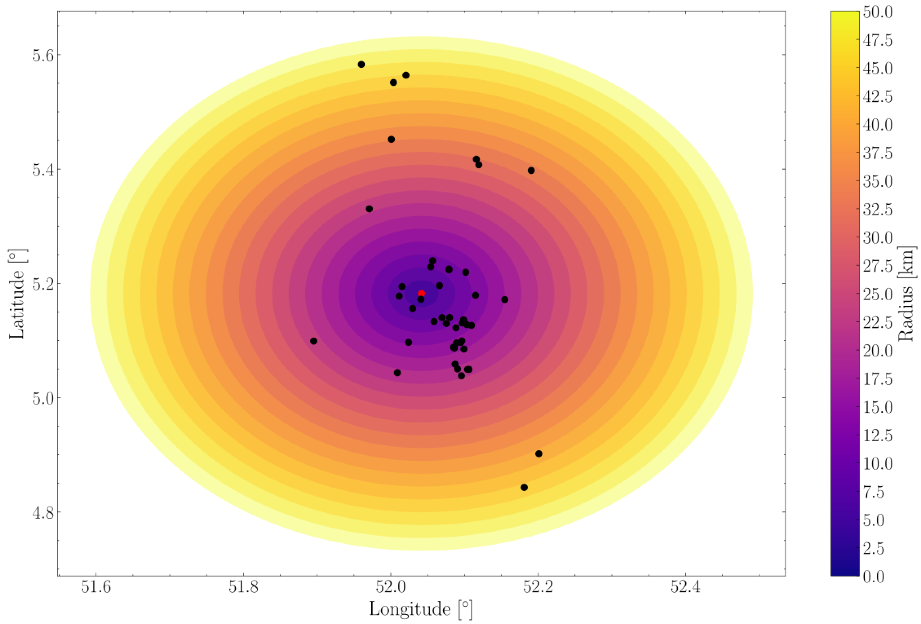
Figure 2.
Distribution of MAE values as a function of the number of neighboring PV installations included.
Figure 2.
Distribution of MAE values as a function of the number of neighboring PV installations included.
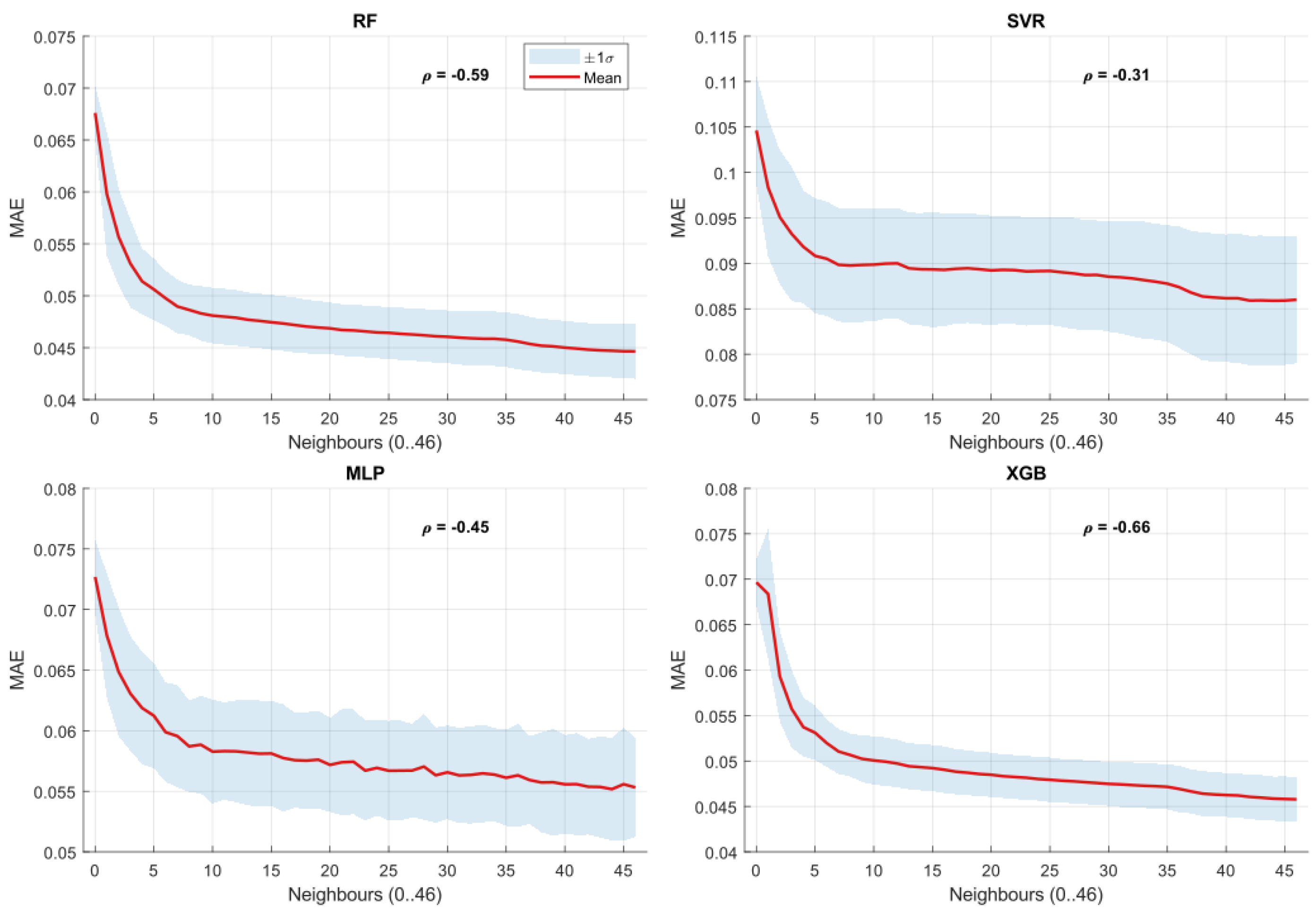
Figure 3.
Distribution of RMSE values as a function of the number of neighboring PV installations included.
Figure 3.
Distribution of RMSE values as a function of the number of neighboring PV installations included.
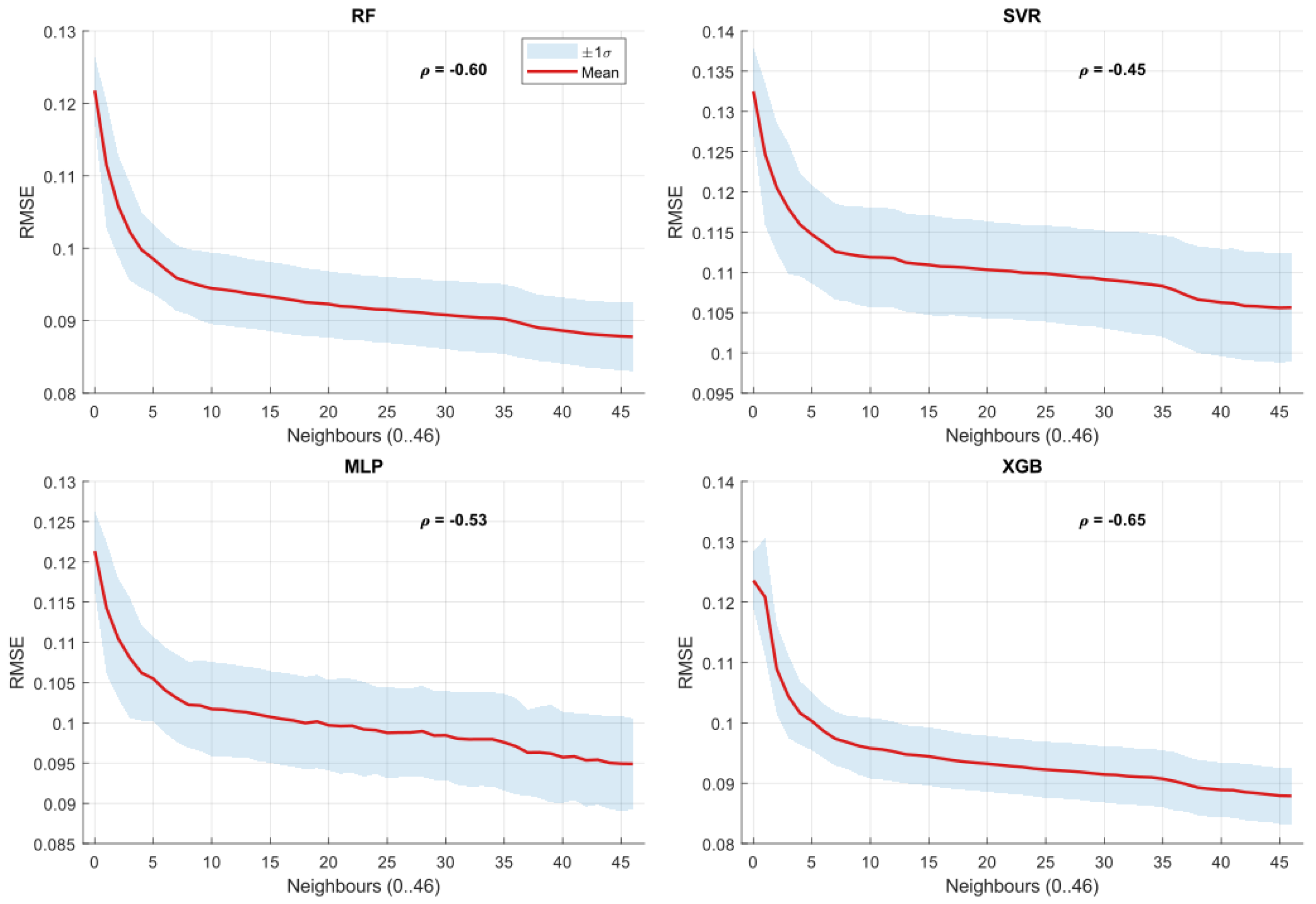
Figure 4.
Distribution of values as a function of the number of neighboring PV installations included.
Figure 4.
Distribution of values as a function of the number of neighboring PV installations included.
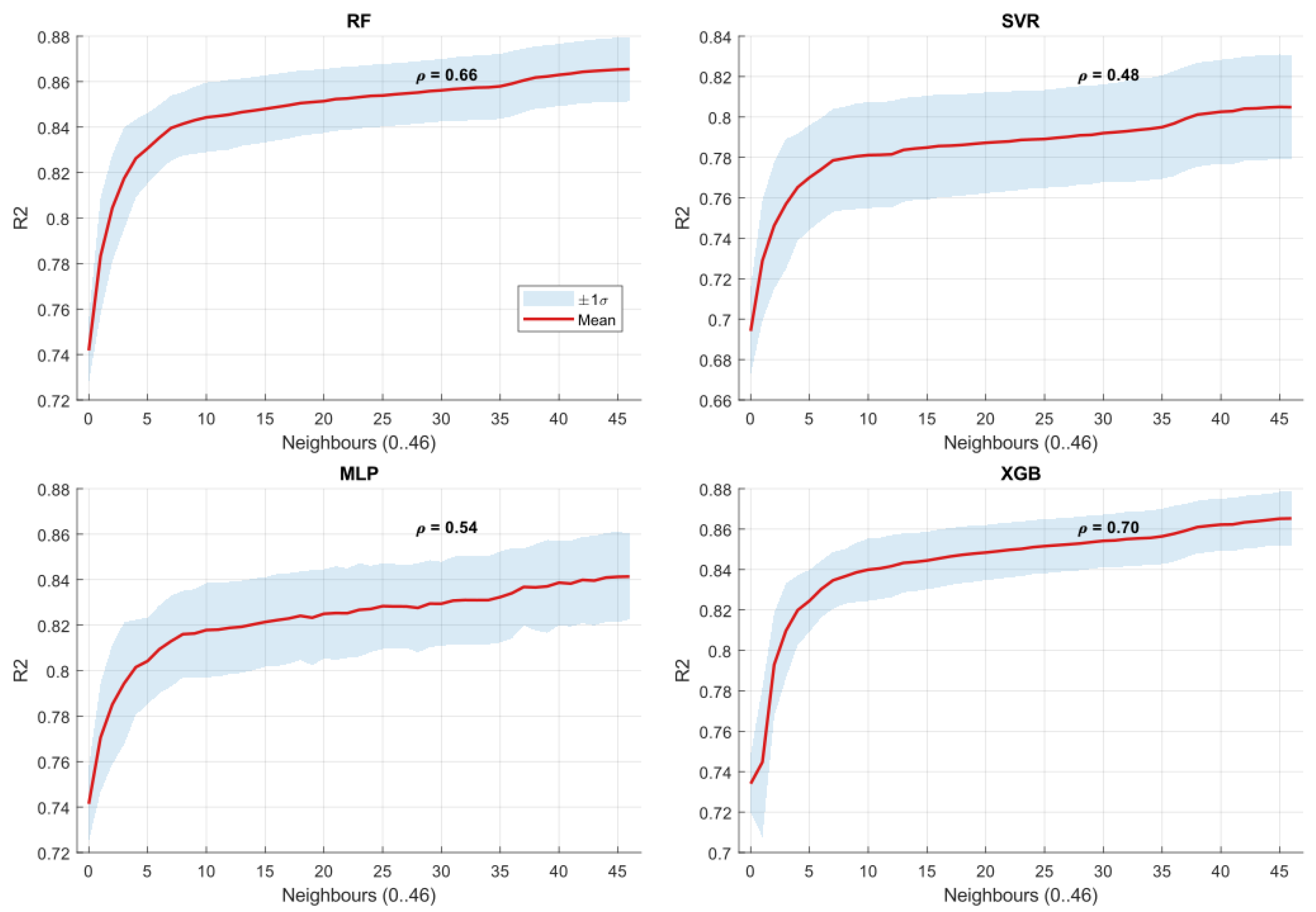
Figure 5.
Economic cost (EUR) as a function of the number of neighboring PV installations included
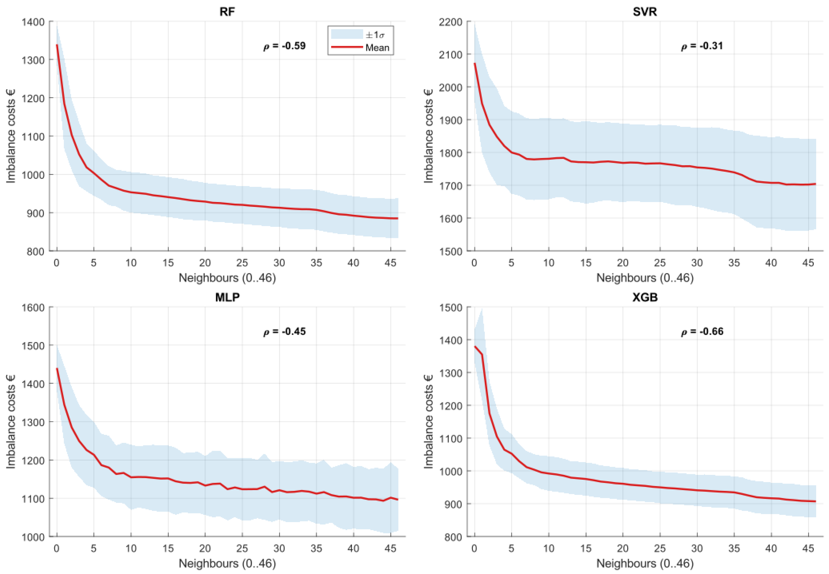
Figure 6.
Marginal Benefit versus Number of Participating PV Systems
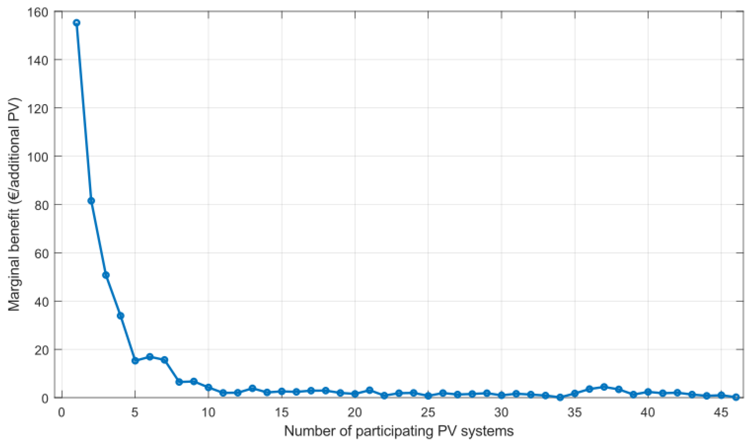
Figure 7.
Average number of neighbors as a function of radius
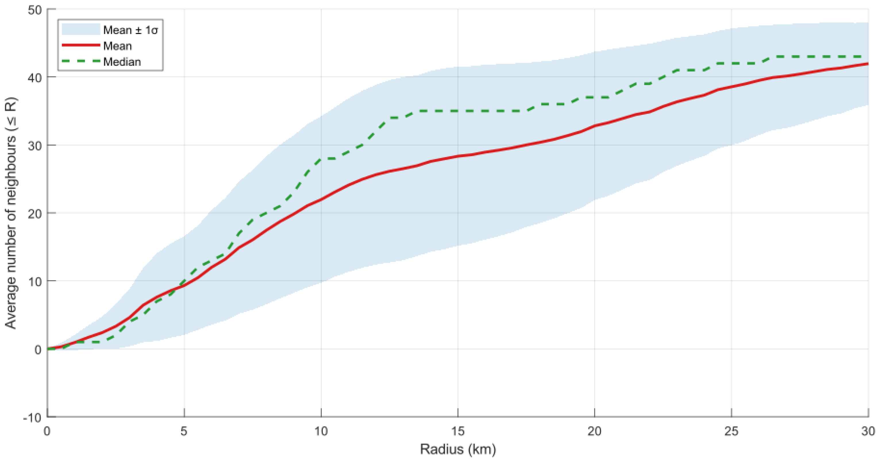
Table 1.
Hyperparameter configurations and search ranges for machine learning models.
| Model | RF (Random Forest) |
|---|---|
| Hyperparameters | n_estimators, max_depth, min_samples_split, min_samples_leaf, bootstrap, max_features |
| Search range | 100–500, 3–20, 2–10, 1–4, {True,False}, {sqrt,log2} |
| Model | XGB (XGBoost) |
| Hyperparameters | learning_rate, n_estimators, max_depth, subsample, colsample_bytree, reg_alpha, reg_lambda |
| Search range | 0.01–0.3, 100–500, 3–15, 0.7–1.0, 0.7–1.0, 0–1, 0–1 |
| Model | SVR |
| Hyperparameters | C, gamma, kernel, epsilon |
| Search range | 0.1–10, {scale,auto}, {rbf,linear}, 0.01–0.1 |
| Model | MLP |
| Hyperparameters | hidden_layer_sizes, activation, solver, alpha, learning_rate_init, early_stopping |
| Search range | {(32,), (64,), (32,32), (64,64)}, {relu,tanh}, adam, 0.0001–0.1, 0.001–0.01, {True,False} |
| Training config. | TimeSeriesSplit(n_splits=5), random_state=42, n_jobs=-1, scoring=MAE, n_iter=50 |
Table 2.
Distribution statistics of forecasting performance metrics across PV installations using the Haurwitz clear-sky GHI model.
Table 2.
Distribution statistics of forecasting performance metrics across PV installations using the Haurwitz clear-sky GHI model.
| Metric | Mean | Standard Deviation |
|---|---|---|
| MAE | 0.0817 | 0.0045 |
| RMSE | 0.1488 | 0.0075 |
| 0.6313 | 0.0407 |
Table 3.
Forecasting accuracy for evaluated models at Level 2 (mean ± std across PV units).
| Model | MAE | RMSE | |
|---|---|---|---|
| AVG | 0.0795 ± 0.0040 | 0.1496 ± 0.0062 | 0.6416 ± 0.0222 |
| SVR | 0.1046 ± 0.0060 | 0.1325 ± 0.0054 | 0.6941 ± 0.0215 |
| RF | 0.0676 ± 0.0026 | 0.1218 ± 0.0047 | 0.7418 ± 0.0140 |
| XGB | 0.0697 ± 0.0026 | 0.1236 ± 0.0048 | 0.7340 ± 0.0145 |
| MLP | 0.0727 ± 0.0031 | 0.1213 ± 0.0050 | 0.7414 ± 0.0164 |
Table 5.
Imbalance costs at different network densities (Random Forest model).
| Network Configuration | Imbalance Cost (€) |
|---|---|
| Level 2 (0 neighbors) | 1339 |
| Level 3 (5 neighbors) | 1260 |
| Level 3 (10 neighbors) | 1210 |
| Level 3 (15 neighbors) | 1190 |
| Level 3 (46 neighbors) | 1175 |
Table 6.
Neighborhood Density Evolution with Increasing Radius
| Radius (km) | Mean | Median | Std Dev | Network Phase |
|---|---|---|---|---|
| 2.5 | 3.32 | 2.00 | 3.30 | Immediate neighborhood |
| 5.0 | 9.32 | 10.00 | 7.26 | Local cluster formation |
| 7.5 | 16.04 | 19.00 | 10.29 | Cluster integration |
| 10.0 | 21.96 | 28.00 | 12.26 | Regional network |
| 15.0 | 28.34 | 35.00 | 13.17 | Near-complete connectivity |
| 20.0 | 32.81 | 37.00 | 10.90 | Saturation phase |
| 30.0 | 41.96 | 43.00 | 6.07 | Full network integration |
Disclaimer/Publisher’s Note: The statements, opinions and data contained in all publications are solely those of the individual author(s) and contributor(s) and not of MDPI and/or the editor(s). MDPI and/or the editor(s) disclaim responsibility for any injury to people or property resulting from any ideas, methods, instructions or products referred to in the content. |
© 2025 by the authors. Licensee MDPI, Basel, Switzerland. This article is an open access article distributed under the terms and conditions of the Creative Commons Attribution (CC BY) license (http://creativecommons.org/licenses/by/4.0/).
Copyright: This open access article is published under a Creative Commons CC BY 4.0 license, which permit the free download, distribution, and reuse, provided that the author and preprint are cited in any reuse.


