
Submitted:
03 November 2025
Posted:
04 November 2025
You are already at the latest version
Abstract
Transformers for time series forecasting rely on positional encoding to inject temporal order into the permutation-invariant self-attention mechanism. Classical sinusoidal absolute encodings are fixed and purely geometric; learnable absolute encodings often overfit and fail to extrapolate, while relative or advanced schemes can impose substantial computational overhead without being sufficiently tailored to temporal data. This work introduces a family of window-statistics positional encodings that explicitly incorporate local temporal semantics into the representation of each timestamp. The base variant (WinStat) augments inputs with statistics computed over a sliding window; WinStatLag adds explicit lag-difference features; and hybrid variants (WinStatFlex, WinStatTPE, WinStatSPE) learn soft mixtures of window statistics with absolute, learnable, and semantic positional signals, preserving the simplicity of additive encodings while adapting to local structure and informative lags. We evaluate proposed encodings on four heterogeneous benchmarks against state-of-the-art proposals: Electricity Transformer Temperature (hourly variants), Individual Household Electric Power Consumption, New York City Yellow Taxi Trip Records, and a large-scale industrial time series from heavy machinery. All experiments use a controlled Transformer backbone with full self-attention to isolate the effect of positional information. Across datasets, the proposed methods consistently reduce mean squared error and mean absolute error relative to a strong Transformer baseline with sinusoidal positional encoding and state-of-the-art encodings for time series, with WinStatFlex and WinStatTPE emerging as the most effective variants. Ablation studies that randomly shuffle decoder inputs markedly degrade the proposed methods, supporting the conclusion that their gains arise from learned order-aware locality and semantic structure rather than incidental artifacts. A simple and reproducible heuristic for setting the sliding-window length—roughly one quarter to one third of the input sequence length—provides robust performance without the need for exhaustive tuning.
Keywords:
time series
; transformer
; positional encoding
; embedding
; local context
1. Introduction
The proliferation of sensors, Internet of Things (IoT) devices, and large-scale digital infrastructures has exponentially increased the availability of multivariate and high-frequency time series, thereby broadening the potential and the challenges of Time Series Forecasting (TSF). TSF has become a cornerstone of contemporary artificial intelligence research, with a wide spectrum of applications in domains such as energy demand management [1], climate modeling [2], financial prediction [3], healthcare monitoring [4], and intelligent transportation systems [5]. of TSF [6,7,8]. Within this context, evolving from classical statistical methods, such as AutoRegressive Integrated Moving Average (ARIMA) [9], towards machine learning and deep learning approaches that can capture nonlinear dependencies and complex temporal dynamics [7,8].
TSF methods have evolved over the past several decades from classical statistical models to machine learning and, more recently, deep learning approaches [10]. Statistical methods, such as ARIMA, modeled linear temporal dynamics under stationarity assumptions, while subsequent machine learning techniques (e.g., gradient boosting trees) enabled more flexible nonlinear pattern modeling. The advent of deep learning introduced sequence-based models, notably recurrent neural networks (RNNs) and long-short-term memory (LSTM) networks. These kinds of methods equipped TSF with long-term memory that can be learned, while convolutional neural networks (CNN) captured local temporal patterns. However, CNNs cannot effectively capture global or long-range temporal dependencies, and RNN/LSTM-based models often struggle to model very long sequences due to vanishing gradients and computational constraints. To address these limitations, attention-based Transformer models have emerged as a powerful alternative, leveraging self-attention mechanisms to model long-term dependencies across time steps [11].
Transformers have achieved state-of-the-art performance in TSF, particularly for long-horizon forecasting tasks, by capturing global temporal relationships that eluded earlier methods. Unlike RNNs, the Transformer’s self-attention is permutation-invariant and does not inherently encode temporal order, so Transformer-based TSF models rely heavily on positional encoding schemes to inject sequence ordering information. Recent research underscores that the design of these positional encoding strategies is both crucial and challenging for time series data [12]. Likewise, the authors in [7] observed that the efficacy of different positional encoding methods in time series remains an open question, with debates over the best approaches (absolute vs. relative encoding). Thus, despite the success of Transformer models in TSF due to their ability to model long-term dependencies, they introduce new challenges stemming from their heavy reliance on positional encoding strategies for temporal-order modeling.
Numerous efforts have been devoted to refining and enhancing positional encoding to preserve the sequential coherence inherent in time-series data. Several variants have been proposed to improve adaptability to the data and strengthen locality and semantic characteristics. For example, time Absolute Positional Encoding (tAPE) [7] adapts the encoding frequencies to the length of the input sequence to preserve distance-awareness, while Relative Positional Encoding (RPE) [13] seeks to capture correspondences between different points in the series. Nonetheless, these methods remain heavily dependent on a static geometric component. To overcome this limitation, alternatives such as Temporal Positional Encoding (TPE) [8] —which introduces a semantic dimension—or Learnable Positional Encodings (LPE) [14] have been explored. Although these methods promise performance gains, their outcomes are often unstable due to increased computational demands, difficulties in constraining values within a normalized range, and sensitivity to initialization.
In light of these challenges, the investigation and development of novel positional encoding mechanisms specifically designed for TSF is an open challenge, addressed in this paper. The motivation is twofold: first, to overcome the limitations of fixed encodings, which often fail to capture the dynamic and nonlinear temporal relationships inherent in multivariate and high-frequency series; and second, to enable Transformer-based models to learn the best positional representation during training for the given task. By allowing encodings to adjust to the underlying temporal structure of each dataset, the WinStat family aim to improve the model’s capacity to capture both local and long-range dependencies, thereby improving forecasting accuracy and robustness. The effectiveness of these learnable positional encodings will be tackled through comprehensive experimental evaluations on widely used TSF benchmarks, comparing their performance with established absolute and relative encoding strategies.
These experiments demonstrate that, across diverse forecasting benchmarks—from household power consumption and transformer load monitoring to urban taxi demand and large-scale industrial sensor streams—the proposed WinStat positional encodings consistently outperform both classic sinusoidal and purely learnable schemes. In particular, WinStatFlex and WinStatTPE yield average reductions in mean squared error of 10–30% and exhibit up to 90% improvement in high-precision settings relative to a strong Informer baseline. Notably, in certain cases, the WinStat base variant also surpasses the baseline, emerging as a competitive third alternative within the family. Moreover, ablation analyses with decoder-input shuffling confirm that these gains arise from meaningful order-aware locality and semantic context rather than incidental artifacts. Such results validate our hypothesis that integrating local window statistics and adaptive positional signals offers a robust and effective approach to TSF with Transformers.
The rest of this paper is organized as follows. Section 2 reviews the evolution of time series forecasting methods and the role of positional encodings in Transformer architectures. Section 3 introduces our WinStat family of window-statistics–based positional encodings, detailing the base WinStat model and its Lag, Flex, TPE, and SPE variants. Section 4 describes the datasets, model configuration, data preprocessing, and evaluation protocols used to ensure fair comparison across encoding schemes. Section 5 presents a comprehensive experimental evaluation using four diverse forecasting benchmark datasets. Section 5.3 includes ablation studies with shuffled inputs to validate the semantic contribution of each encoding. Finally, Section 6 offers concluding remarks, highlights the key findings, and outlines promising directions for future research.
2. Background
TSF has undergone a profound evolution, driven by the growing ubiquity of complex temporal data in science, industry, and everyday life. In this section, we present an overview of the methodological advances that have shaped the field, tracing the progression from classical statistical models and machine learning approaches to the recent dominance of deep learning and Transformer-based architectures. We focus particularly on the role of positional encoding mechanisms, which are crucial for adapting permutation-invariant self-attention to the inherently ordered nature of time series, setting the stage for our proposed enhancements in later sections.
2.1. Time Series Forecasting
TSF has long been a fundamental problem in statistics, econometrics, and, more recently, artificial intelligence. Its goal is to estimate the future evolution of a temporal signal based on historical data, enabling informed decision-making in various domains, including energy demand management, finance, traffic prediction, healthcare, and climate science. Classical approaches, such as ARIMA [9] and exponential smoothing methods such as Prophet [15], are grounded in linear modeling assumptions and stationarity. These models provide interpretable components –trend, seasonality, and residuals– and remain valuable baselines. However, they often fail in the presence of strong non-linearity, abrupt changes, and complex multivariate dependencies.
With the increasing availability of high-frequency and multivariate data, machine learning approaches such as support vector regression and gradient boosting machines [16] gained popularity due to their ability to approximate non-linear functions without strict assumptions. These models improved robustness across heterogeneous datasets, but are limited by their reliance on manually designed features and their difficulty in capturing sequential dependencies across long time horizons.
The deep learning era brought about a paradigm shift in TSF. Sequence models such as RNNs and their gated variants – LSTMs and Gated Recurring Units (GRUs) – became the dominant architectures for sequential data [17]. These models utilize recurrent connections to maintain a hidden state over time, allowing for modeling of long-term dependencies. At the same time, CNNs demonstrated strong performance on temporal data, exploiting their inductive bias to capture local patterns and hierarchical representations [18]. However, these architectures exhibit limitations. CNNs are constrained by fixed receptive fields, while RNNs struggle with vanishing gradients and scalability to very long sequences. These shortcomings became particularly evident in long-term forecasting scenarios, where the accumulation of errors and the limited temporal context severely degrade performance.
2.2. Transformers for TSF
Transformers, introduced by Vaswani et al. [19], represent a breakthrough in sequence modeling by replacing recurrence and convolutions with the self-attention mechanism. This design enables parallelization during training, efficient handling of long dependencies, and the ability to model pairwise interactions between all elements in a sequence. The success of Transformers in natural language processing and computer vision has inspired their adaptation to TSF, where capturing both short- and long-range temporal dependencies is crucial.
Transformer-based TSF varies its approach from sparsity-driven efficiency to structure and variable-aware designs. LogTrans [20] first relaxed the quadratic self-attention bottleneck by introducing LogSparse patterns, with memory efficiency, together with convolutional self-attention to inject locality. Informer [21] then proposed ProbSparse attention to reach time and memory complexity, added self-attention distilling to handle extreme input lengths, and used a generative-style decoder to predict the full horizon in one forward pass. Moving beyond sparsity, Autoformer [22] embedded seasonal-trend decomposition and replaced point-wise attention with Auto-Correlation mechanism (computed via Fast Fourier Transform) to capture period-based dependencies with complexity. In parallel, Pyraformer [23] adopted a pyramidal multiresolution attention graph that shortens the maximum signal path to complexity while keeping the time and memory complexity of . Building on decoposition-based designs, FedFormer [24] brought frequency-domain blocks (Fourier and Wavelet) and mixture-of-experts decomposition, achieving linear complexity by selecting a fixed number of frequency modes. Triformer [25] targeted multivariate settings with a triangular, patch-based attention of linear complexity and variable-specific parametrization, improving the modeling of important variable dynamics over long horizons. More recently, Ister [26] advanced decomposition-based approaches by inverting the seasonal trend framework and employing a dual transformer with dot-attention, improving interpretability and efficiency while capturing multi-periodic patterns. In parallel, Gateformer [27] focused on multivariate forecasting through a dual-stage design that encodes temporal dynamics within each variable and applies gated cross-variate attention, yielding significant performance gains across diverse datasets.
Despite these architectural innovations, the effectiveness of Transformers for long-term forecasting has been questioned. Zeng et al. [6] demonstrated that embarrassingly simple linear models (LTSF-Linear) outperform sophisticated Transformer variants across multiple benchmarks, suggesting that many proposed designs may not truly capture temporal relations but rather exploit dataset-specific properties. This debate highlights that while Transformers offer powerful modeling capabilities, their application to TSF requires careful design, including the integration of inductive biases such as decomposition, spectral analysis, or position-awareness, to ensure robust temporal modeling.
2.3. Positional Encoding Approaches in Transformers for TSF
A central challenge in adapting Transformers to time series lies in their permutation-invariant self-attention mechanism. Since the model lacks an inherent notion of order, positional encodings (PEs) are crucial for injecting temporal information into the input. Early approaches used absolute sinusoidal encodings, while recent research has explored learnable, relative, and hybrid methods, each with advantages and limitations [8]. We summarize the main contributions in the state-of-the-art as follows, whilst Table 1 summarizes the main positional encoding strategies proposed in the literature for time series models, highlighting whether they are fixed or learnable, how they inject positional information, and their relative advantages.
2.3.1. Positional Encodings
Here, we review both absolute and relative encodings, both fixed and learnable, that embed each time step with index-based signals added directly to input representations. Although these methods offer simplicity and efficient extrapolation, they often lack adaptability to the rich nonlinear dynamics present in real-world temporal data.
Absolute Positional Encoding (APE). The original absolute encoding proposed by Vaswani et al. [19] defines position-dependent vectors using sinusoidal functions:
where denotes the position index and i the embedding dimension. These encodings are fixed and parameter-free, allowing extrapolation to unseen lengths. LPE replace trigonometric functions with trainable parameters, granting the flexibility of the model but sacrificing extrapolation [14]. For time series, Foumani et al. [7] introduced the time Absolute Position Encoding (tAPE), which adjusts frequency terms to incorporate sequence length L:
thereby preserving distance awareness even for low-dimensional embeddings.
Relative Positional Encoding (RPE). RPE capture the distance between elements, rather than their absolute positions. Shaw et al. [13] formulated the attention score as:
where encodes the relative offset between positions i and j. The output of the attention is defined as:
This provides translation invariance and improves generalization when relative lags are more important than absolute timestamps. Foumani et al. [7] further proposed an efficient Relative PE (eRPE), which reduces the memory cost of naive implementations.
2.3.2. Hybrid and Advanced Encodings
Although absolute and relative encodings capture complementary aspects of positional information, recent research has introduced hybrid and more advanced schemes that combine or extend their strengths.
Transformer with Untied Positional Encoding (TUPE). Ke et al. [28] proposed TUPE, which modifies the attention formulation by incorporating both absolute and relative terms, but with untied parameters between the query, key, and positional embeddings. Instead of simply adding position vectors to the input embeddings, TUPE directly introduces them into the attention computation:
where and are positional embeddings and , are learnable position-specific projections. This untied design allows queries and keys to interact with both content and positional signals independently, providing more expressive control over position modeling.
Rotary Position Embedding (RoPE). Su et al. [29] introduced Rotary Position Embeddings (RoPE), which encode absolute positions through rotation in a complex plane. The idea is to apply a position-dependent rotation matrix to the query and key vectors before computing attention:
where is a block-diagonal matrix performing 2D rotations with angle . The inner product then becomes:
thus encoding relative positions implicitly through multiplicative phase shifts. RoPE naturally preserves distance-awareness and enables extrapolation.
Temporal Positional Encoding (T-PE). Irani and Metsis [8] described a hybrid scheme (T-PE) that augments absolute sinusoidal encodings with a semantic similarity kernel across time steps. Specifically:
where is the absolute positional encoding of index i, and the Gaussian kernel captures local similarity in the embedding space. This formulation allows the model to combine global periodic signals with local contextual information. Although powerful, it scales quadratically with the sequence length.
Representative and Global Attention. Alioghli and Okay [30] proposed two variants of relative positional encoding, tailored for anomaly detection and time series tasks.
Representative Attention partitions the sequence into local neighborhoods and assigns a representative positional embedding to each group g. The attention score between the token i and j becomes:
where is the representative embedding of the group containing position j. This formulation reduces sensitivity to small offsets and is particularly effective for short sequences.
Global Attention introduces a single global positional embedding g that interacts with all queries and keys, capturing long-range dependencies. The score is modified as:
where g acts as a learnable global anchor. This scheme emphasizes global coherence across the entire sequence, making it better suited for long horizons.
Both methods extend the relative encoding family by biasing attention scores toward either local (Representative) or global (Global) temporal contexts, thus adapting positional awareness to different forecasting regimes.
2.4. Limitations of Previous Positional Encoding Approaches for TSF
Despite the progress achieved by absolute, relative, and hybrid positional encodings, several limitations remain when applying them to TSF. Fixed absolute encodings, such as the sinusoidal functions introduced by Vaswani et al. [19], are attractive because they are parameter-free and allow extrapolation to unseen sequence lengths. However, they lack any adaptivity to the underlying temporal dynamics of the data. This rigidity becomes particularly problematic in TSF, where sampling frequencies and temporal dependencies vary greatly across domains. Moreover, at low embedding dimensions, sinusoidal encodings suffer from anisotropy, producing highly correlated vectors that diminish the model’s ability to distinguish between positions [7].
Learnable Absolute Encodings (LPE) [14] attempt to address this by allowing position vectors to be optimized during training. While this improves flexibility, it also sacrifices extrapolation capacity, since learned encodings are tied to the maximum sequence length observed during training. Consequently, they can overfit to specific horizons and degrade in generalization performance when deployed on longer forecasting tasks. Similarly, methods such as tAPE [7] adjust frequencies according to sequence length to improve distance-awareness, but they remain deterministic and do not fully capture dataset-specific temporal structures.
Relative Positional Encodings (RPEs) [13] alleviate some of these issues by focusing on temporal offsets rather than absolute indices, improving translation invariance and often delivering better performance in tasks where relative lags are critical. However, standard implementations require memory and computation, severely limiting scalability to long sequences, being L the sequence length and d the dimension of the embedding. Efficient variants, such as eRPE [7], reduce this overhead but at the cost of architectural complexity and potential information loss. Hybrid approaches, including TUPE [28], RoPE [29], and T-PE [8], enrich positional information by combining absolute and relative signals or by encoding positions as rotations. Although these strategies offer improved expressiveness, they introduce significant additional computational costs and are not specifically designed to address the challenges of forecasting multivariate high-frequency time series. Furthermore, recent empirical studies [6,30] have revealed that many positional encodings display inconsistent performance across benchmarks, with no single approach emerging as clearly superior.
Taken together, these weaknesses highlight a critical research gap: Current positional encoding schemes either lack adaptivity, impose excessive computational demands, or fail to generalize across forecasting horizons and datasets. For time series forecasting, which often involves complex non-linear dependencies, irregular sampling, and diverse temporal patterns, there is a need for encodings that can (i) exploit local statistical context, (ii) capture temporal lag structures, and (iii) flexibly combine multiple sources of positional information. This motivates the family of proposals introduced in this work, WinStat, which aim to unify these requirements into a set of encodings that are learnable, efficient, and semantically meaningful for forecasting tasks.
3. WinStat Positional Encoding Family
In this section, we present a novel family of positional encoding strategies—collectively termed WinStat (short for Window-based Statistics)—that explicitly incorporates local temporal context into Transformer-based forecasting models. Building on the observation that classical sinusoidal encodings capture only global, index-based geometry, and that purely learnable or relative schemes either overfit or incur prohibitive overhead, WinStat instead augments each timestamp’s embedding with summary statistics computed over a sliding window and, in extended variants, with short-term lag differences. We further introduce hybrid formulations that learn optimal mixtures of these window-based signals with traditional absolute and semantic similarity encodings, allowing the model to adaptively weight global periodicity, local variability, and context-dependent similarity. By maintaining the simplicity of additive encoding while injecting richer temporal semantics, our approach aims to enhance the Transformer’s ability to model both local and long-range dependencies in diverse time series forecasting tasks.
3.1. WinStat base
The first proposed method, WinStat, defines our most basic positional encoding method. WinStat enriches each input embedding by concatenating local statistics computed over a sliding window of size w. For each position t, we calculate:
where is the neighborhood window centered at t.
The statistical vector obtained is:
and the enriched embedding would be:
where the operation ‖ notes the vector concatenation operation. The enriched sequence is noted as:
3.2. WinStatLag
WinStatLag extends WinStat by incorporating explicit temporal lag differences. Given a set of lags , for each position t we compute:
The enriched embedding becomes:
where and meets that . Thus, the sequence is:
This formulation captures both local statistics and short- to medium-term variations, providing richer semantic context.
3.3. WinStatFlex
WinStatFlex generalizes the approach by combining WinStatLag with several additive positional encodings using trainable weights. Specifically, given encodings (sinusoidal), (learnable), (time-aware), and (temporal hybrid), the final representation is:
where ensures normalized, sum-one trainable weights. This design allows the model to learn the optimal contribution of statistical, lag-based, and additive encodings, adapting to dataset-specific requirements.
3.4. WinStatTPE
WinStatTPE follows the same weighted scheme as WinStatFlex but replaces with . This substitution exploits the hybrid nature of TPE, combining absolute sinusoidal structure with local semantic similarity:
The learnable weights control the balance between global periodicity, local statistics, and semantic similarity, making this variant particularly robust.
3.5. WinStatSPE
Finally, WinStatSPE integrates the WinStatFlex scheme with Stochastic Positional Encoding (SPE), a convolution-based modification of the attention matrix. The enriched embedding is:
where denotes the previous additive components, the weights are a sum-one normalized vector, and introduces convolutional structure in the attention mechanism. Although SPE is primarily designed for classification, its integration here allows an exploratory assessment of its potential for forecasting.
4. Experimental Set-up
In this section, we describe the experimental framework designed to evaluate the effectiveness of the proposed WinStat family of positional encodings against established baselines. Our evaluation strategy emphasizes controlled comparisons by maintaining identical architectural configurations across all variants, thereby isolating the effect of positional information on forecasting performance. We conduct experiments on four heterogeneous benchmarks that span different domains, sampling frequencies, and temporal characteristics: residential energy consumption (HPC), electricity infrastructure monitoring (ETT), urban mobility patterns (NYC), and industrial machinery monitoring (TINA). These datasets collectively provide a comprehensive testbed for assessing the robustness and generalizability of our approach across diverse time series forecasting scenarios. The experimental design follows rigorous protocols for temporal data, including chronological splitting to preserve sequential dependencies and systematic hyperparameter selection guided by preliminary sensitivity analyses.
4.1. Datasets
To comprehensively evaluate the proposed WinStat family of positional encodings, we selected four heterogeneous time series datasets that span different domains, temporal granularities, and forecasting challenges. These benchmarks were chosen to assess robustness across varied data characteristics: from high-frequency household consumption data (HPC) to electrical grid monitoring with strong seasonal patterns (ETT), urban mobility aggregates (NYC), and large-scale industrial sensor streams (TINA). Each dataset presents distinct temporal dynamics—ranging from clear periodicity to mixed stationary-nonstationary behavior—ensuring that our positional encoding methods are tested under diverse forecasting scenarios representative of real-world applications.
(HPC)
The Individual Household Electric Power Consumption dataset (UCI) records minute-level consumption for a household near Paris from December 2006 to November 2010 (47 months; timestamps) [31]. Although UCI lists nine attributes, the date and time fields are stored separately; when unified, each timestamp comprises eight variables (time plus seven electrical measurements). HPC blends clearly seasonal components (e.g., sub-metering channels) with variables closer to stationarity (e.g., reactive power), and shows strong associations between global active power and intensity. This combination of high frequency, long duration and mixed temporal behavior makes HPC a demanding benchmark for positional encodings intended to capture both local and global temporal structure.
Electricity Transformer Dataset (ETT)
The ETT benchmark, popularized by Informer and subsequent TSF studies, records load components and oil temperature (OT) from two power transformers installed in different substations [21,32]. The public release comprises two minute-level series (ETT-small-m1, ETT-small-m2; 2 years, timestamps each) and their hourly counterparts (ETTh1, ETTh2) that downsample the same process to reduce computational burden [32]. Each timestamp contains eight features (time plus seven variables: HUFL, HULL, MUFL, MULL, LUFL, LULL, and OT). Empirically, ETTh1 exhibits marked seasonality and high one-step autocorrelation across variables, whereas ETTh2 retains seasonality with smaller amplitudes—differences that make ETTh2 comparatively harder to model. The OT variable is operationally salient because extreme temperatures impact transformer health and efficiency, which turns the dataset into a meaningful testbed for long-horizon forecasting under strong periodic structure.
Yellow Trip Data (NYC)
The Yellow Trip Data Records from NYC Open Data provide hourly aggregates of operational and monetary variables (e.g., passenger count, trip distance, fare amount, tip amount, total amount) [33]. In our setup, the 2015 series were preprocessed and then artificially extended to exceed two million timestamps to broaden temporal coverage while keeping moderate dimensionality (time + six variables). Autocorrelation analyses reveal pronounced daily periodicities (e.g., peaks around workday transitions in passenger_count and fare_amount), cross-variable synchrony (e.g., tip_amount with passenger_count/fare_amount), and near-stationary components (e.g., trip_distance).
Time-series Industrial Anomaly (TINA)
TINA is an industrial multivariate time series released by DaSCI for anomaly analysis in heavy machinery [34]. Data were collected from a mining machine at ArcelorMittal every two seconds between 2017-09-06 and 2018-12-25, yielding roughly 38 million timestamps. After anonymization and normalization, the dataset contains 108 columns (numeric and categorical), including categorical indicators such as FEATURE76, FEATURE87, maintenance flags (m_id, m_subid), and alarms. Its scale and heterogeneity make TINA an exacting test for both computational efficiency and robustness of positional encodings for TSF, particularly under the presence of rare, high-impact events.
4.2. Model Used and Rationale
As backbone, we adopt an Informer-like Transformer - chosen for its prevalence in the TSF literature and practical tooling - while disabling ProbSparse to recover vanilla full self-attention. This choice ensures a faithful assessment of positional encodings without confounding effects from sparsification or distillation that may erase locality, which is particularly harmful when encodings inject local statistics or semantic context. Using attention provides a clean, comparable environment to isolate the effect of positional information and test procedures, such as completely removing PE.
Recent advancements in transformer-based models have led to a shift in how positional information is integrated. Positional encoding has increasingly become implicit, often incorporated directly within the architecture rather than explicitly tied to the input data. Contemporary architectures such as PatchTST [35] and TimeNET [36] exemplify this trend: PatchTST employs cross-patch attention and does not rely on explicit positional encodings, while TimeNET omits attention mechanisms entirely, effectively removing traditional positional signals. Consequently, existing approaches do not employ positional encodings in the traditional sense, preventing a straightforward comparison with our proposed methods.
We avoid architectures with implicit positional mechanisms (e.g., auto-correlation–based designs) so that improvements can be attributed to the encoding itself rather than architectural priors. Implementation follows a minimal, modifiable Transformer encoder–decoder stack suitable for multivariate TSF.
4.3. Validation Schema and Evaluation Metrics
To preserve temporal semantics, we use a chronological last-block split for testing and validation. Specifically, we adopt a 70–30 train–test partition and derive validation using a second-to-last block extracted from the training segment. We explicitly avoid blocked cross-validation due to its stationarity requirement and the prohibitive retraining costs associated with long sequences. This protocol yields an unbiased out-of-sample estimate while respecting order constraints.
Finally, dataset-specific horizons and windows follow a lightweight sensitivity study on ETT (e.g., typical setting , , ) and are adapted when memory constraints arise in large and wide data sets (e.g., TINA with , ).
Training minimizes the mean squared error (MSE), the de facto regression loss in TSF, ensuring comparability to previous work. We report MSE and Mean Absolute Error (MAE) as primary metrics.
4.4. Positional-Window Size Selection
All WinStat variants share a single hyperparameter, the window size w, which determines how much local context (statistics and lagged differences) each position receives. Very large windows dilute locality, producing generic statistics that contribute little to attention; very small windows are noise–prone and may hinder pattern detection. Hence, w must balance local sensitivity and robustness.
Exhaustive search over w is prohibitive on large corpora, so we established a practical heuristic with a controlled study on the hourly ETT variants. Using the canonical Informer setting (, , ), we swept on ETTh1 and ETTh2, repeating each configuration 10 times to stabilize the MSE estimates. The best ranges fell between and , i.e., approximately one quarter to one third of the sequence length. We therefore adopt the rule-of-thumb when feasible.
On very large or high-frequency datasets we apply the heuristic subject to memory constraints. For instance, on TINA (sequence length ) the 30-second sampling interval motivates broader context, but GPU memory constraints required us to cap the window at (roughly the last half hour), instead of using –. This preserves informative locality while keeping training feasible.
4.5. Hyperparameters by Dataset
In Table 2, we report the dataset-specific configuration used across all positional-encoding variants so that architectural effects are held constant and differences can be attributed to the encoding itself (Transformer with vanilla self-attention, batch size, dropout, and number of runs as indicated).
4.6. Hardware and Software Framework
All experiments are implemented in Python with PyTorch as the deep learning framework; data handling and analysis rely on NumPy, Pandas, Matplotlib, and statsmodels. Training is carried out in a DGX cluster with 1× NVIDIA Tesla V100 (32 GB), 32 CPU cores (Intel® Xeon® E5-2698) and 96GB RAM. All implementation and experimental setup details are included in GitHub https://github.com/ari-dasci/S-WinStat.
5. Results and Analysis
In this section, we present a comprehensive empirical evaluation of the proposed WinStat family of positional encodings across all available heterogeneous benchmarks. Our experimental design aims to identify overall trends that may indicate the most effective encoding variant across diverse datasets. To this end, we evaluate all five proposed variants on each dataset—HPC, the ETT hourly variants, NYC, and TINA—alongside established baselines, using identical architectural configurations and training protocols to ensure fair comparison. Performance is assessed through MSE and MAE metrics across multiple independent runs. To validate that improvements stem from meaningful positional structure rather than incidental artifacts, we include decoder-input shuffling tests that systematically disrupt temporal order. This ablation approach allows us to establish a causal link between the proposed local semantic encodings and forecasting accuracy, while the learned mixture weights provide interpretable insights into which positional components contribute most effectively to each domain.
5.1. Comparative Results
We use the five previously introduced datasets as a comprehensive testing ground to evaluate the proposed encodings (WinStat, WinStatLag, WinStatFlex, WinStatTPE, WinStatSPE) against established baselines under identical architectural configurations and data splits. Collectively, these datasets constitute a heterogeneous benchmark environment, capturing a wide spectrum of temporal properties such as seasonality, stationarity, locality, and the coexistence of high- and low-frequency information. This diversity provides a rigorous basis for assessing the robustness and generality of the proposed methods across problems with distinct structural and semantic characteristics.
Table 3 consolidates all results across datasets and methods, including Informer (with timeF), sinusoidal APE only, a no-PE ablation, and the WinStat family. Informer serves as the reference baseline, with removal of PE leading to substantial performance degradation (higher MSE/MAE), whereas sinusoidal APE shows moderate gains. Figure 1 shows that, among the WinStat variants, WinStatFlex and WinStatTPE consistently achieve the lowest errors and most stable variances in HPC. Additionally, results on TUPE and ROPE datasets—representative of state-of-the-art benchmarks—confirm that the observed patterns generalize beyond the HPC dataset.
On the ETT hourly benchmarks (ETTh1/ETTh2), both WinStatFlex and WinStatTPE markedly outperform Informer, while the no-PE ablation consistently ranks last, underscoring the necessity of explicit positional information. Figure 2 shows the performance in ETTh1: TUPE situates between WinStatFlex and WinStatTPE, highlighting its intermediate effectiveness. Sinusoidal APE behaves poorly, in some cases even worse than the shuffled WinStat variants, suggesting that purely geometric absolute signals may misalign with the true temporal dependencies of this subset unless complemented by local or semantic components. As shown in Table 3, the ranking for ETTh2, from best to worst, is: WinStatFlex > WinStat base > TUPE > WinStatTPE > WinStatLag, with ROPE performing particularly poorly and occupying the last position. As illustrated in Figure 3, the visual comparison clearly emphasizes this gap, and reveals the high variance in ROPE’s results, underscoring its instability across runs. This confirms that semantic and local positional information, as captured by the WinStat variants, remains critical for accurately modeling long-range dependencies in these datasets.
Regarding the hourly NYC aggregates, we caution that the series was artificially extended, which may bias the metrics toward optimistic values due to the smoothing effects of generative augmentation. With that caveat, WinStat base achieves the best performance overall. WinStatTPE and ROPE show very similar results, while TUPE performs particularly poorly—worse even than the no-PE ablation. WinStatFlex still surpasses Informer and sinusoidal APE, but the ranking highlights that, in this dataset, the effectiveness of positional encoding varies substantially across methods. As shown in Table 3 and Figure 4 and Figure 5, this variability is visually evident, revealing marked contrasts in performance stability between the WinStat family and methods like TUPE. Due to this reason, the figure has been divided to better read the results.
The fourth benchmark, TINA—an industrial, high-dimensional dataset originally curated for anomaly analysis—poses a stringent test of computational efficiency and robustness. Even after careful optimization, its scale requires substantial hardware and long runs; however, its breadth provides a valuable stress test for the positional mechanisms. As summarized in Table 3, the results indicate that, in terms of MSE, WinStat base achieves the best performance, followed closely by ROPE, with Informer slightly behind; WinStatTPE, WinStatFlex, and TUPE all perform worse than Informer. However, when considering MAE, the ranking shifts: WinStatLag becomes the top performer, while WinStatTPE, WinStatFlex, and WinStatBase exhibit very similar results, and TUPE ranks last—even below the no-PE ablation. These fluctuations highlight that the relative effectiveness of positional encodings can vary substantially due to the particular characteristics of this dataset. Graphically, the behavior of the encodings can be observed in Figure 6, where WinStatFlex and WinStatTPE clearly stand out, achieving substantially better results than the other methods. For the remaining models, however, it becomes difficult to establish a clear hierarchy, as the relative performance varies depending on the metric considered.
5.2. Analysis of the Learned Mixture Weights
To gain a clearer insight into the internal behavior of the proposed encodings, we analyze the relative contribution of each component within the normalized weighting scheme of WinStatFlex and WinStatTPE. For this purpose, we compile tables reporting the normalized weights associated with each component, enabling us to assess their relative importance in the overall computation. This analysis allows us to identify which parts dominate the representation and to evaluate whether the observed weighting patterns align with the intended design of the encodings.
HPC
The learned mixture weights, as reported in Table 4, indicate that the strongest variants assign non-trivial mass to the local-statistics component together with absolute/learnable encodings (and, for TPE, a semantic term), rationalizing their superiority over fixed APE.
ETT
In the case of the ETT benchmarks, both datasets exhibit a fairly similar and balanced behavior. For the first subset, ETTh1 (Table 5), and the WinStatFlex variant, the statistical component is marginally higher than the others, although the relevance distribution remains close to one-fourth across all components. For WinStatTPE, this slight increase shifts toward the TPE component itself, potentially due to its semantic contribution, which facilitates the modeling of outcomes. Overall, however, the weighting can be described as nearly uniform across components for both variants. This effect becomes even more pronounced in ETTh2 (Table 6), where both models achieve values that closely approximate an equal proportionality among components.
Yellow Trip Data (NYC): Aggregated Urban Mobility
Learned mixture weights, as reported in Table 7, show non-trivial mass on Stats and TPE, indicating that local statistics and semantic similarity are the dominant contributors in this domain. In this case, the differences among components are more pronounced than in the previous datasets. For the WinStatFlex variant, Stats and tAPE gain greater relevance, reducing the proportional weight of the fixed encoding, which appears to contribute little useful information. For WinStatTPE, the emphasis again falls on the semantic components, namely Stats and TPE. Interestingly, however, the learnable encoding becomes the least relevant component in this setting, which slightly increases the relative importance of the fixed PE.
TINA (Industrial): High-Dimensional, Long Sequences
In the particular case of the TINA dataset, the differences among variants are even more pronounced. For WinStatFlex, the largest share of the weighting falls on the concatenated statistical values, as the high complexity of the time series and its specific characteristics make the semantic information provided by this component especially critical. The tAPE component, despite being specifically designed to adapt the traditional encoding to the properties of the series, does not appear to achieve the intended effect, possibly introducing desynchronization and thus ranking last in relevance. For WinStatTPE, however, the differences among components are minimal, potentially due to the strong semantic contribution of the involved components, but also as a result of the particular characteristics of this dataset.

Table 8.
TINA: learned mixture weights in WinStat variants (normalized). The symbol * identifies a component not considered in the weighting definition.
Table 8.
TINA: learned mixture weights in WinStat variants (normalized). The symbol * identifies a component not considered in the weighting definition.
| Component | WinStatFlex | WinStatTPE |
|---|---|---|
| Stats | 0.3814 | 0.2630 |
| PE | 0.2752 | 0.2450 |
| LPE | 0.1918 | 0.2290 |
| tAPE | 0.1515 | * |
| TPE | * | 0.2630 |
Lessons learned from weight training
After estimating the weights associated with each of the methods integrated into WinStat, several noteworthy conclusions can be drawn. First, the results highlight the high adaptability of WinStat, which stems from the diversity of its constituent components. This adaptability is clearly illustrated by the heatmap in Figure 7, which highlights the substantial variation in weights across different datasets. The visualization makes it evident that the algorithm is capable of dynamically adjusting its weighting strategy according to the characteristics of each specific scenario. Such flexibility is a desirable property in practical applications, as it enhances the robustness and generalizability of the method across heterogeneous contexts.
In addition, the statistical computation component emerges as particularly influential, consistently receiving a relatively high share of importance. For instance, in both the TINA and HPC datasets, this component accounts for more than 30% of the total weight, thereby reinforcing its central role in the overall performance of the framework. The prominence of this component indicates that the extraction and processing of statistical information remain a key driver of predictive capacity within the WinStat architecture.
At the same time, a certain degree of uniformity in the choice of weights is observed across several datasets. This tendency suggests that, while the algorithm adapts to scenario-specific requirements, it also identifies stable patterns of relevance among its components. Taken together with the strong performance metrics consistently achieved by the proposed method, these observations emphasize not only the complementary nature of the individual components but also their collective contribution to the effectiveness of WinStat. Consequently, the results provide empirical support for the design choices underlying the framework and point to its potential applicability in a wide range of real-world tasks.
5.3. Comparing the Semantic Quality of the Encoding
In this Section, we highlight the semantic role of positional encodings and their importance for evaluating encoding quality. Although semantics lie outside the architecture, whose layers process only numerical tensors, such information may be implicitly captured through locality and patterns, which our proposed encodings aim to exploit.
A straightforward way to assess this is to shuffle the decoder inputs during inference and compare the performance with intact sequences, as suggested in [6]. This procedure provides an intuitive measure of whether an encoding preserves order and locality, as a significant drop in performance indicates that the model relies on sequential structure to make accurate predictions. In contrast, if shuffling has little effect, it suggests that the encoding does not effectively capture temporal dependencies.
To examine this property, we employed the five datasets evaluated previously, selected to study the impact of input shuffling across problems with diverse temporal and semantic characteristics, particularly in terms of seasonality and stationary patterns. The decoder shuffling procedure was applied to the WinStat family, as well as to TUPE, ROPE, and the Informer model itself, enabling a direct comparison of its effect across these different approaches.
As shown in Table 9, the performance of the original Informer and its shuffled variant is nearly identical, which is consistent with the findings of the original study in [6]. The version without positional encoding performs at an intermediate level, leading to overall similar results across all three models and underscoring the limited semantics and weak-order preservation provided by the traditional sinusoidal scheme.
In contrast, WinStatFlex exhibits a marked drop in performance when inputs are shuffled, a desirable behavior that reflects its ability to capture both contextual dependencies and the intrinsic sequential structure of the data.
A similar but more pronounced effect is observed for WinStatTPE, whose degradation under shuffling clearly exceeds that of the baseline Informer. This outcome indicates that the semantic information captured by T-PE is even more sensitive to disorder, highlighting its superior ability to encode a meaningful temporal structure compared to the traditional approach.
Although these two methods achieved the best results in the previous experiments within our model family, the remaining variants exhibit a consistent pattern: all experience a substantial performance degradation when input shuffling is applied. This provides empirical evidence, in a general sense, that our proposed encodings are significantly sensitive to structural changes in the data. Consequently, it demonstrates that they successfully inject meaningful positional information with a strong semantic component into the datasets.
Across the evaluated benchmarks, WinStat base consistently demonstrates superior performance on the TINA and NYC, reflecting the particular temporal characteristics of these series. In TINA, the time series exhibits complex, low-frequency fluctuations over a wide temporal range, making the statistical component especially critical for capturing relevant patterns. In Taxi, the synthetic extension of the series similarly emphasizes the importance of statistical features, helping to stabilize learning despite the artificial augmentation. In contrast, TUPE and ROPE consistently display a counterintuitive behavior on these same datasets: applying input shuffling leads to better performance than the unshuffled model, contrary to the expected clear degradation. This can be attributed both to the distinct nature of these mechanisms—being more strongly driven by attention computations than by the explicit encoding itself—and to the specific characteristics of the datasets. The smoothing effects in Taxi and the wide-ranging fluctuations in TINA reduce the direct impact of positional information on performance, highlighting a fundamental difference compared to the WinStat family, whose encodings are more robustly anchored in the statistical and semantic structure of the data.
We can analyze the differential behavior graphically by examining visualizations that compare the original and shuffled models across the evaluated datasets. In these representations, higher values indicate better performance, meaning that semantic and ordering information is being effectively injected into the model. These visual comparisons highlight how the encoding methods from WinStat family impact the model’s ability to capture meaningful temporal or structural dependencies across datasets.
First, the HPC dataset exhibits minimal differences between the original and shuffled Informer model, as illustrated in Figure 8, which is particularly noteworthy and indicates the limited ordinal information contributed by this approach. A similar behavior is observed for the other tested methods, TUPE and ROPE. In contrast, all four WinStat variants show a substantially larger differential, highlighting a strong ordinal contribution to the model that is effectively disrupted when input shuffling is applied.
For ETTh1 and ETTh2, the observed results differ considerably. In ETTh1, as shown in Figure 9, input shuffling imposes a substantial penalty on Informer, although this effect is smaller in terms of MAE compared to the WinStat family. TUPE, in contrast, exhibits almost negligible degradation, while ROPE even shows a negative difference, indicating better performance under shuffling than in the original configuration, which suggests that this method is not well suited for this dataset. In ETTh2, illustrated in Figure 10, the behavior shifts: WinStatFlex now suffers the largest degradation (in contrast to WinStatLag in ETTh1). Most notably, ROPE exhibits a pronounced negative delta, reflecting a substantial improvement under shuffling. As these experiments were repeated multiple times, this is not an artifact, but rather a clear indication that this mechanism is ineffective for the ETTh2 dataset.
The NYC dataset, shown in Figure 11, exhibits one of the largest discrepancies observed in this experiment, with the WinStatFlex encoding achieving a difference on the order of . This represents, without doubt, the most pronounced result across all benchmarks. Although similar trends can be identified in other models within the WinStat family, the magnitude of the difference in this case is considerably greater, highlighting the distinct sensitivity of this dataset to the proposed encoding.
Finally, as illustrated in Figure 12, in the TINA dataset, several encodings—such as ROPE, TUPE, and the original Informer—exhibit negative differences, meaning that the shuffled models actually outperform their unshuffled counterparts. While this behavior is theoretically counterintuitive, it reinforces the notion that these positional encoding mechanisms are not well suited to the specific characteristics of this dataset. In contrast, all variants of the WinStat family display the expected degradation under shuffling—most notably WinStatTPE—thereby confirming their stronger capacity to encode meaningful positional and semantic information.
6. Conclusions and Future Work
This work examined positional information in Transformer-based time series forecasting and identified a central limitation of classical absolute encodings: they inject only global, index-based geometry and omit local temporal semantics. To address this gap, we introduced window-statistics positional signals and additive, learnable mixtures that combine heterogeneous encodings within a single embedding. These designs enrich each timestamp with local descriptive context (e.g., mean, dispersion, extremes, short-term differences) and allow the model to learn how much to trust absolute, learnable, and semantic components, thereby aligning positions with similar behavior across the series.
Across multiple benchmarks, the proposed encodings consistently improved accuracy over a strong Transformer baseline (Informer). The average gains typically ranged from 10% to 30%, with high-precision regimes exhibiting improvements up to about 90% relative to baseline. The overall ranking places the proposed WinStatFlex encoding as the top performer, followed by WinStatBase, with WinStatTPE emerging as a close alternative that exhibits low variance and stable performance across runs.
Shuffle-based stress tests further confirmed that the benefits come from the learned order-sensitive local/semantic structure. When decoder inputs were randomly permuted, the advantage of the proposed encodings collapsed, while conventional baselines like Informer, TUPE and ROPE were less sensitive to permutation. From a practical standpoint, the only extra hyperparameter shared by the window variants is the window length. A dedicated pre-experiment on ETTh1/ETTh2 suggested a simple, reproducible heuristic to bound this choice without exhaustive search, striking a trade-off between overly generic statistics (large windows) and noisy, uninformative context (small windows). Furthermore, the additive mixture with trainable weights improved performance without requiring the practitioner to hand-tune component balances; softmax normalization provided stable training dynamics.
Several directions emerge naturally. First, extend the proposed positional mechanisms beyond forecasting to time-series classification and anomaly detection, where localized patterns and semantics are equally critical (e.g., medical signals or industrial monitoring). Second, broaden empirical coverage with domains such as medicine, physics, and meteorology to distill cross-domain regularities and simplify the mixture. Third, explore hybridization with frequency-domain architectures (e.g., Fourier/Wavelet-based modules) to learn positional structure across temporal and spectral representations. Finally, investigate distributed and federated training to mitigate the higher training cost and enable privacy-preserving deployment across sites with sensitive data.
Author Contributions
Conceptualization, Ignacio Aguilera-Martos, Diego García-Gil and Julián Luengo; Data curation, Ignacio Aguilera-Martos; Formal analysis, Cristhian Moya-Mota; Funding acquisition, Julián Luengo; Investigation, Cristhian Moya-Mota; Methodology, Ignacio Aguilera-Martos, Diego García-Gil and Julián Luengo; Project administration, Julián Luengo; Software, Cristhian Moya-Mota; Supervision, Diego García-Gil; Validation, Cristhian Moya-Mota; Writing – original draft, Cristhian Moya-Mota, Ignacio Aguilera-Martos, Diego García-Gil and Julián Luengo; Writing – review & editing, Ignacio Aguilera-Martos, Diego García-Gil and Julián Luengo.
Funding
This work was supported by the Spanish Ministry of Science and Technology under grants PID2023-150070NB-I00 and TED2021-132702B-C21 funded by MICIU/AEI/10.13039/501100011033 and by “ERDF/EU” and the “European Union NextGenerationEU/PRTR” respectively. Ignacio Aguilera-Martos was supported by the Ministry of Science of Spain under the FPI programme PRE2021-100169.
Data Availability Statement
All data will be available under request through the corresponding author. Most datasets used are open and appropriately cited in the manuscript. All implementation and experimental setup details are included in GitHub https://github.com/ari-dasci/S-WinStat.
Conflicts of Interest
The authors declare no conflicts of interest.
References
- Palma, G.; Chengalipunath, E.S.J.; Rizzo, A. Time series forecasting for energy management: Neural circuit policies (ncps) vs. long short-term memory (lstm) networks. Electronics 2024, 13, 3641. [Google Scholar] [CrossRef]
- Rezaei, Z.; Samghabadi, S.S.; Amini, M.A.; Shi, D.; Banad, Y.M. Predicting Climate Change: A Comparative Analysis of Time Series Models for CO2 Concentrations and Temperature Anomalies. Environmental Modelling & Software 2025, p. 106533.
- Buczyński, M.; Chlebus, M.; Kopczewska, K.; Zajenkowski, M. Financial time series models—comprehensive review of deep learning approaches and practical recommendations. Engineering Proceedings 2023, 39, 79. [Google Scholar] [CrossRef]
- He, R.; Chiang, J.N. Simultaneous forecasting of vital sign trajectories in the ICU. Scientific Reports 2025, 15, 14996. [Google Scholar] [CrossRef] [PubMed]
- Cheng, C.H.; Tsai, M.C.; Cheng, Y.C. An intelligent time-series model for forecasting bus passengers based on smartcard data. Applied Sciences 2022, 12, 4763. [Google Scholar] [CrossRef]
- Zeng, A.; Chen, M.; Zhang, L.; Xu, Q. Are Transformers Effective for Time Series Forecasting? In Proceedings of the AAAI Conference on Artificial Intelligence. AAAI, 2023, Vol. 37, pp. 11121–11128.
- Foumani, N.M.; Tan, C.W.; Webb, G.I.; Salehi, M. Improving position encoding of transformers for multivariate time series classification. Data Mining and Knowledge Discovery 2024, 38, 22–48. [Google Scholar] [CrossRef]
- Irani, H.; Metsis, V. Positional Encoding in Transformer-Based Time Series Models: A Survey. arXiv preprint arXiv:2502.12370 2025.
- Ariyo, A.A.; Adewumi, A.; Ayo, C. Stock price prediction using the ARIMA model. In Proceedings of the 2014 UKSim-AMSS 16th International Conference on Computer Modelling and Simulation. IEEE, 2014, pp. 106–112.
- Liu, X.; Wang, W. Deep time series forecasting models: A comprehensive survey. Mathematics 2024, 12, 1504. [Google Scholar] [CrossRef]
- Su, L.; Zuo, X.; Li, R.; Wang, X.; Zhao, H.; Huang, B. A systematic review for transformer-based long-term series forecasting. Artificial Intelligence Review 2025, 58, 80. [Google Scholar] [CrossRef]
- Oliveira, J.M.; Ramos, P. Evaluating the effectiveness of time series transformers for demand forecasting in retail. Mathematics 2024, 12, 2728. [Google Scholar] [CrossRef]
- Shaw, P.; Uszkoreit, J.; Vaswani, A. Self-Attention with Relative Position Representations. In Proceedings of the 2018 Conference of the North American Chapter of the Association for Computational Linguistics: Human Language Technologies, Volume 2 (Short Papers). Association for Computational Linguistics, 2018, pp. 464–468.
- Devlin, J.; Chang, M.W.; Lee, K.; Toutanova, K. BERT: Pre-training of deep bidirectional transformers for language understanding. In Proceedings of the NAACL-HLT, 2019, pp. 4171–4186.
- Taylor, S.J.; Letham, B. Forecasting at scale. The American Statistician 2017, 72, 37–45. [Google Scholar] [CrossRef]
- Friedman, J.H. Greedy function approximation: A gradient boosting machine. Annals of Statistics 2001, 29, 1189–1232. [Google Scholar] [CrossRef]
- Bahdanau, D.; Cho, K.; Bengio, Y. Neural machine translation by jointly learning to align and translate. arXiv preprint arXiv:1409.0473 2014.
- Bai, S.; Kolter, J.Z.; Koltun, V. An empirical evaluation of generic convolutional and recurrent networks for sequence modeling. In Proceedings of the 35th International Conference on Machine Learning (ICML), 2018, pp. 481–490.
- Vaswani, A.; Shazeer, N.; Parmar, N.; Uszkoreit, J.; Jones, L.; Gomez, A.N.; Kaiser, Ł.; Polosukhin, I. Attention is all you need. In Proceedings of the Advances in Neural Information Processing Systems, 2017, Vol. 30.
- Li, S.; Jin, X.; Xuan, Y.; Zhou, X.; Chen, W.; Wang, Y.X.; Yan, X. Enhancing the locality and breaking the memory bottleneck of transformer on time series forecasting. In Proceedings of the Advances in Neural Information Processing Systems, 2019, number 32, pp. 5243–5253.
- Zhou, H.; Zhang, S.; Peng, J.; Zhang, S.; Li, J.; Xiong, H.; Zhang, W. Informer: Beyond efficient transformer for long sequence time-series forecasting. In Proceedings of the AAAI Conference on Artificial Intelligence, 2021, Vol. 35, pp. 11106–11115.
- Xu, J.; Wu, H.; Wang, J.; Long, M. Autoformer: Decomposition transformers with auto-correlation for long-term series forecasting. In Proceedings of the Advances in Neural Information Processing Systems, 2021, Vol. 34, pp. 22419–22430.
- Liu, M.; Zeng, A.; Chen, M.; Xu, Q. Pyraformer: Low-complexity pyramidal attention for long-range time series modeling and forecasting. In Proceedings of the International Conference on Learning Representations, 2021.
- Zhou, H.; Zhang, S.; Peng, J.; Zhang, S.; Li, J.; Xiong, H.; Zhang, W. FEDformer: Frequency enhanced decomposed transformer for long-term series forecasting. In Proceedings of the International Conference on Machine Learning, 2022, pp. 27268–27286.
- Cirstea, R.G.; Bica, I.; van der Schaar, M. Triformer: Triangular, variable-specific attentions for long sequence multivariate time series forecasting. In Proceedings of the International Joint Conference on Artificial Intelligence, 2022, pp. 2054–2060.
- Cao, F.; Yang, S.; Chen, Z.; Liu, Y.; Cui, L. Ister: Inverted Seasonal-Trend Decomposition Transformer for Explainable Multivariate Time Series Forecasting. arXiv preprint arXiv:2412.18798 2024.
- Lan, Y.H. Gateformer: Advancing Multivariate Time Series Forecasting via Temporal and Variate-Wise Attention with Gated Representations. In Proceedings of the 1st ICML Workshop on Foundation Models for Structured Data.
- Ke, G.; He, D.; Liu, T.Y. Rethinking Positional Encoding in Language Pre-training. In Proceedings of the International Conference on Learning Representations (ICLR), 2021.
- Su, J.; Lu, Y.; Pan, S.; Wen, B.; Liu, Y. RoFormer: Enhanced Transformer with Rotary Position Embedding. In Proceedings of the Findings of the Association for Computational Linguistics: ACL-IJCNLP 2021. Association for Computational Linguistics, 2021, pp. 683–692.
- Alioghli, A.A.; Okay, F.Y. Enhancing multivariate time-series anomaly detection with positional encoding mechanisms in transformers. The Journal of Supercomputing 2025, 81, 282–306. [Google Scholar] [CrossRef]
- Hebrail, G.; Berard, A. Individual Household Electric Power Consumption. UCI Machine Learning Repository, 2010.
- Zhou, H. ETDataset: A Benchmark Dataset for Time-Series Forecasting. GitHub repository, 2021.
- NYC Open Data – Yellow Taxi Trip Records. City of New York Open Data, 2015.
- Aguilera-Martos, I.; López, D.; García-Barzana, M.; Luengo, J.; Herrera, F. Time-series Industrial Anomaly (TINA) Dataset. DaSCI Institute dataset, 2022.
- Nie, Y.; Nguyen, N.H.; Sinthong, P.; Kalagnanam, J. A Time Series is Worth 64 Words: Long-term Forecasting with Transformers 2023.
- Wu, H.; Hu, T.; Liu, Y.; Zhou, H.; Wang, J.; Long, M. TimesNet: Temporal 2D-Variation Modeling for General Time Series Analysis. In Proceedings of the International Conference on Learning Representations, 2023.
Figure 1.
Mean squared error (MSE) and mean absolute error (MAE) calculated on the HPC dataset for all encodings (Sorted by MAE)
Figure 1.
Mean squared error (MSE) and mean absolute error (MAE) calculated on the HPC dataset for all encodings (Sorted by MAE)
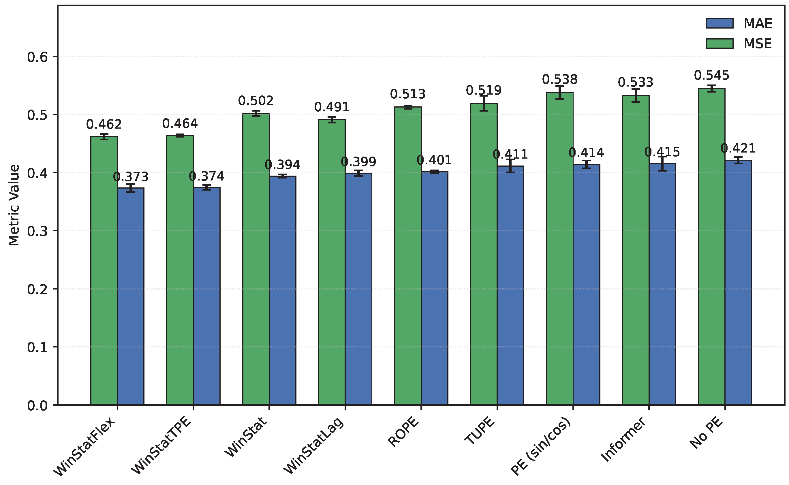
Figure 2.
Mean squared error (MSE) and mean absolute error (MAE) calculated on the ETTh1 dataset for all encodings (Sorted by MAE)
Figure 2.
Mean squared error (MSE) and mean absolute error (MAE) calculated on the ETTh1 dataset for all encodings (Sorted by MAE)
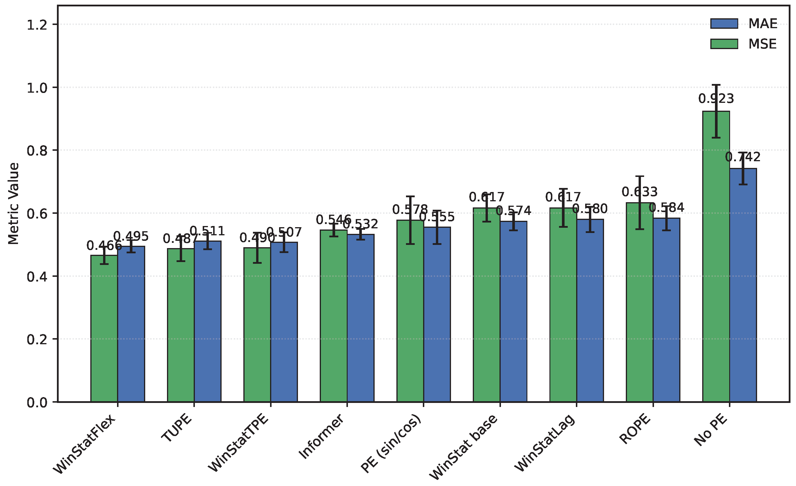
Figure 3.
Mean squared error (MSE) and mean absolute error (MAE) calculated on the ETTh2 dataset for all encodings (Sorted by MAE)
Figure 3.
Mean squared error (MSE) and mean absolute error (MAE) calculated on the ETTh2 dataset for all encodings (Sorted by MAE)
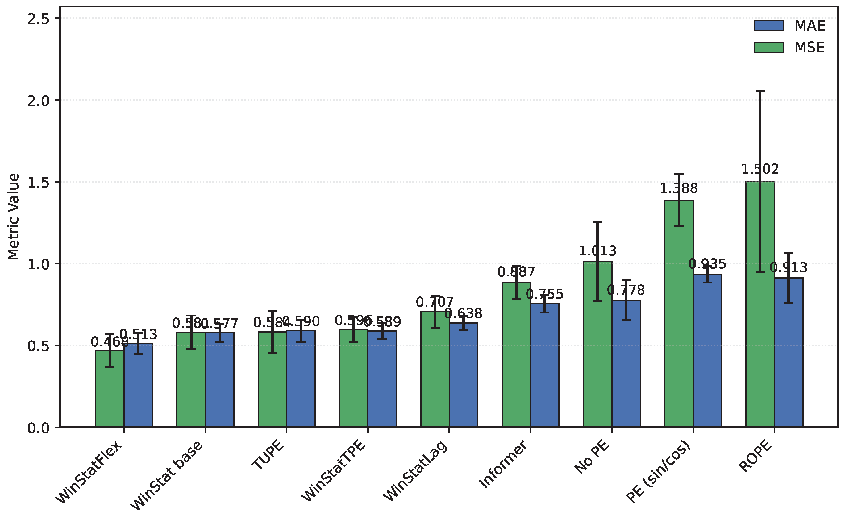
Figure 4.
Mean squared error (MSE) calculated on the NYC dataset for all encodings (Sorted by MSE)
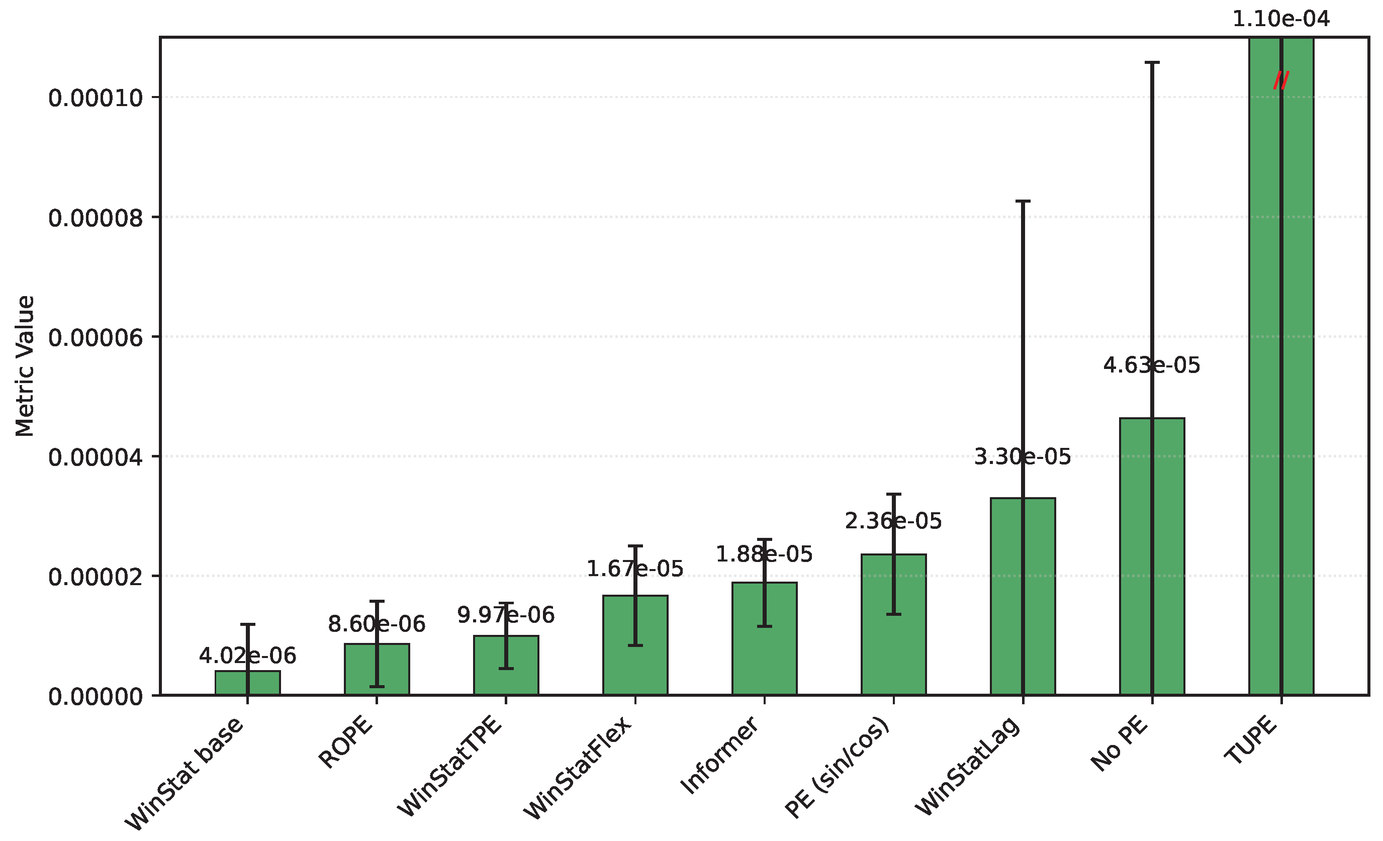
Figure 5.
Mean absolute error (MAE) calculated on the NYC dataset for all encodings (Sorted by MAE)
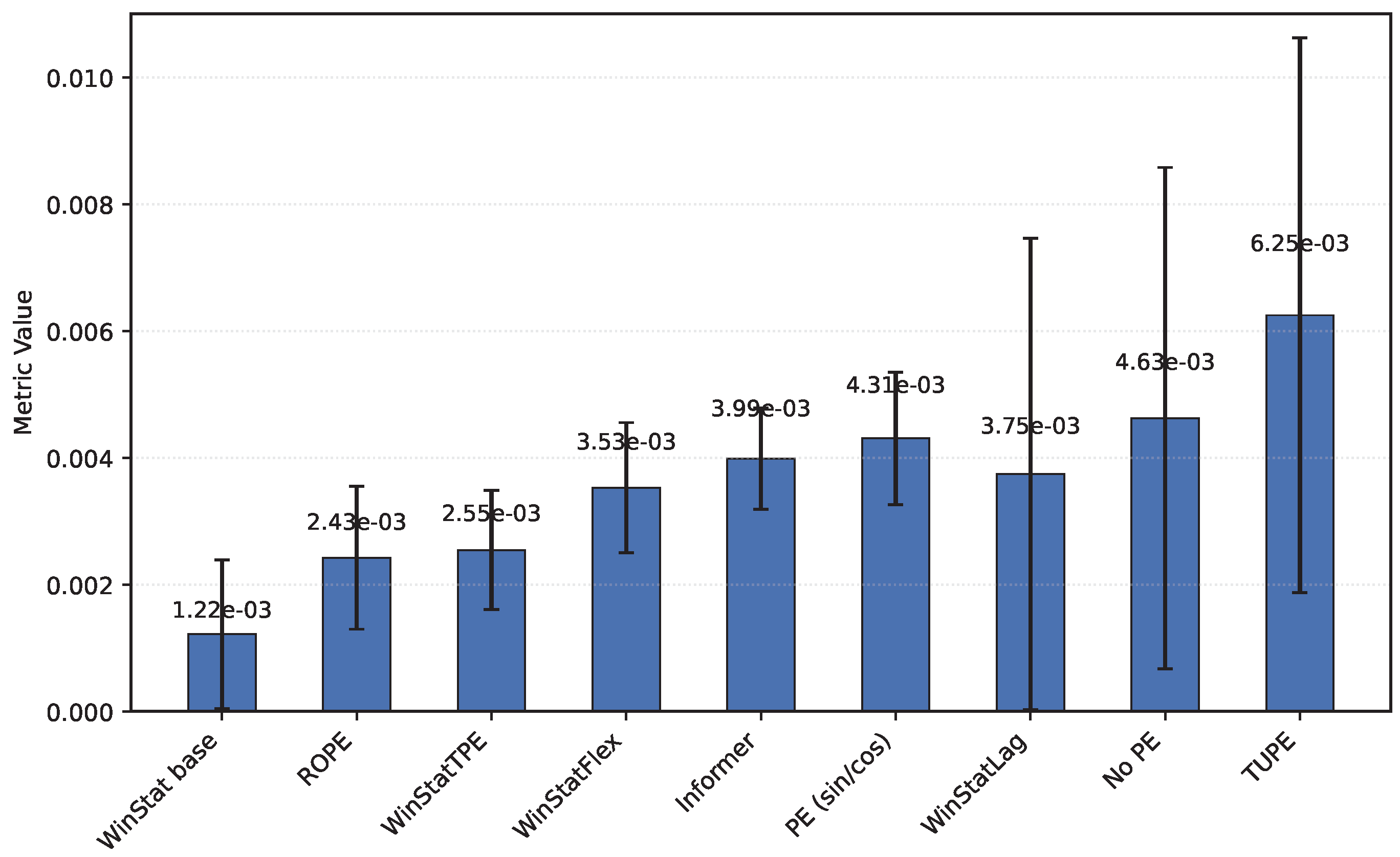
Figure 6.
Mean squared error (MSE) and mean absolute error (MAE) calculated on the TINA dataset for all encodings (Sorted by MAE)
Figure 6.
Mean squared error (MSE) and mean absolute error (MAE) calculated on the TINA dataset for all encodings (Sorted by MAE)
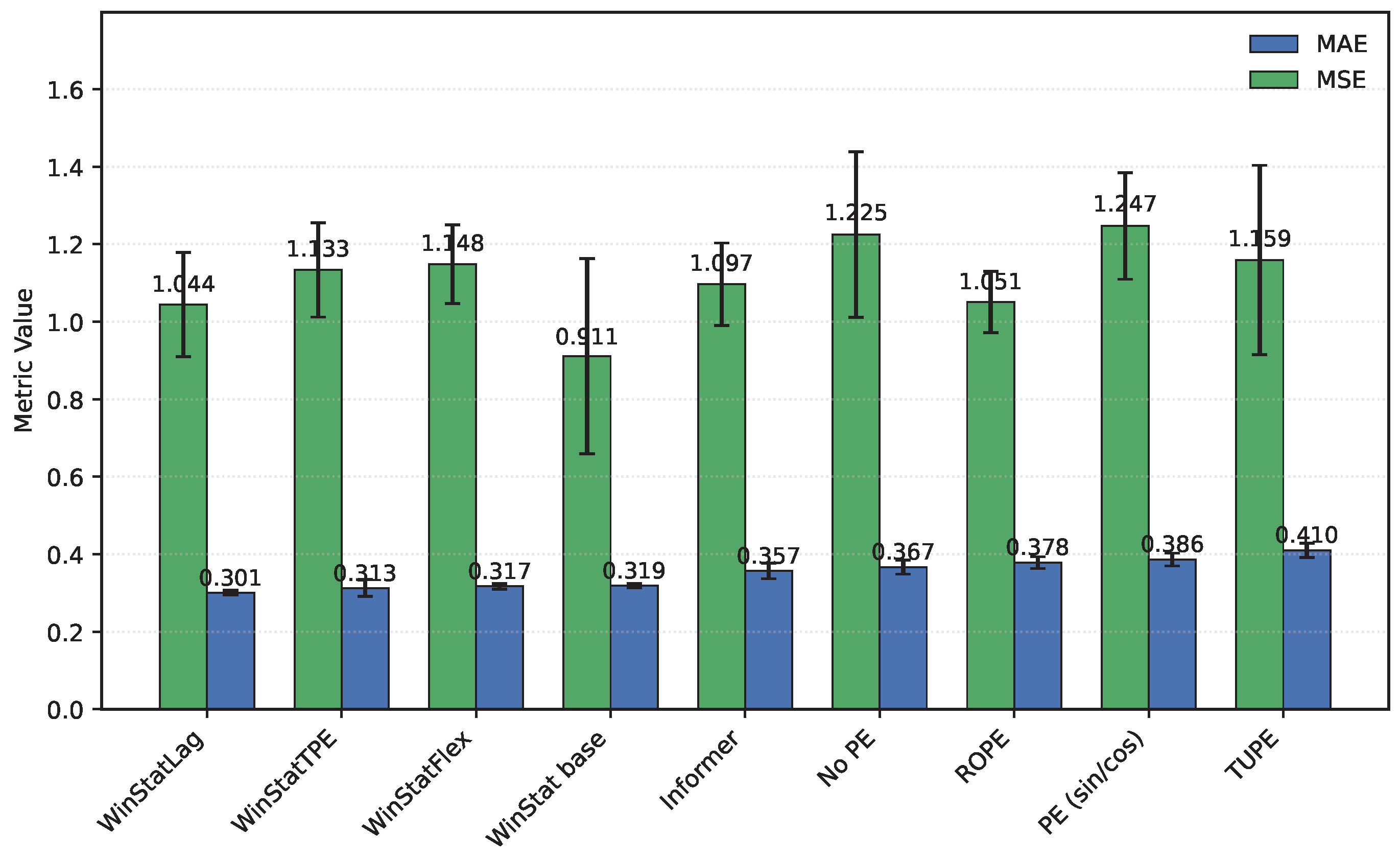
Figure 7.
Component-wise weight values in WinStatFlex and WinStatTPE.
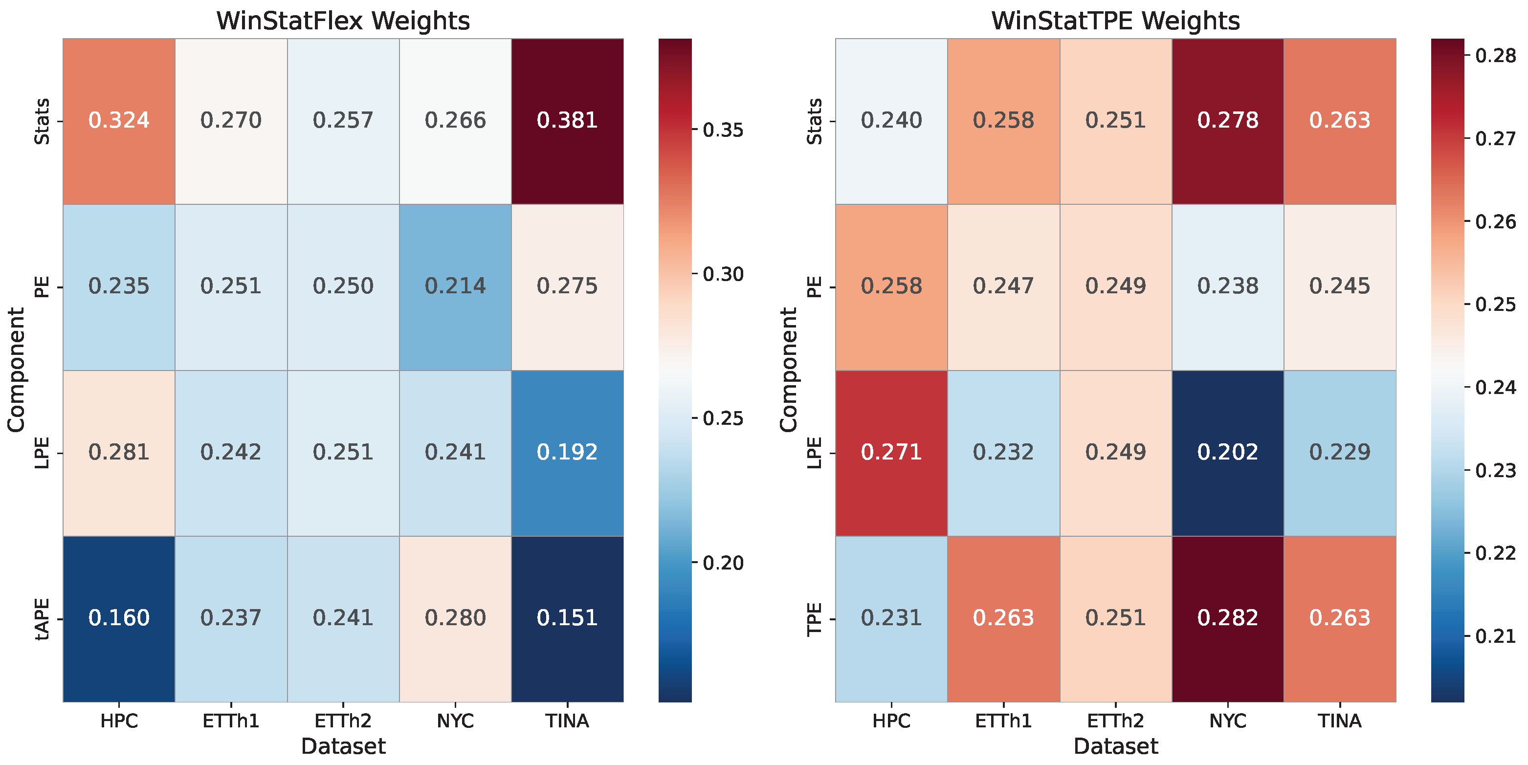
Figure 8.
Comparison of original and shuffled models on the HPC dataset. Higher values indicate better incorporation of semantic and ordering information. A larger difference suggests stronger ordinal dependence of the encoding, which is disrupted when shuffling.
Figure 8.
Comparison of original and shuffled models on the HPC dataset. Higher values indicate better incorporation of semantic and ordering information. A larger difference suggests stronger ordinal dependence of the encoding, which is disrupted when shuffling.
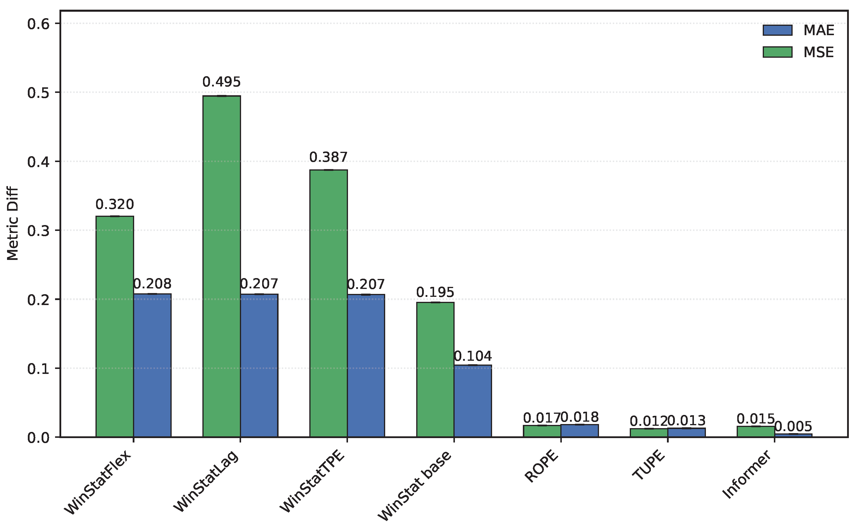
Figure 9.
Comparison of original and shuffled models on the ETTh1 dataset. Higher values better reflect the use of semantic and ordering information. Greater differences reveal stronger ordinal dependence in the encoding, broken by shuffling.
Figure 9.
Comparison of original and shuffled models on the ETTh1 dataset. Higher values better reflect the use of semantic and ordering information. Greater differences reveal stronger ordinal dependence in the encoding, broken by shuffling.
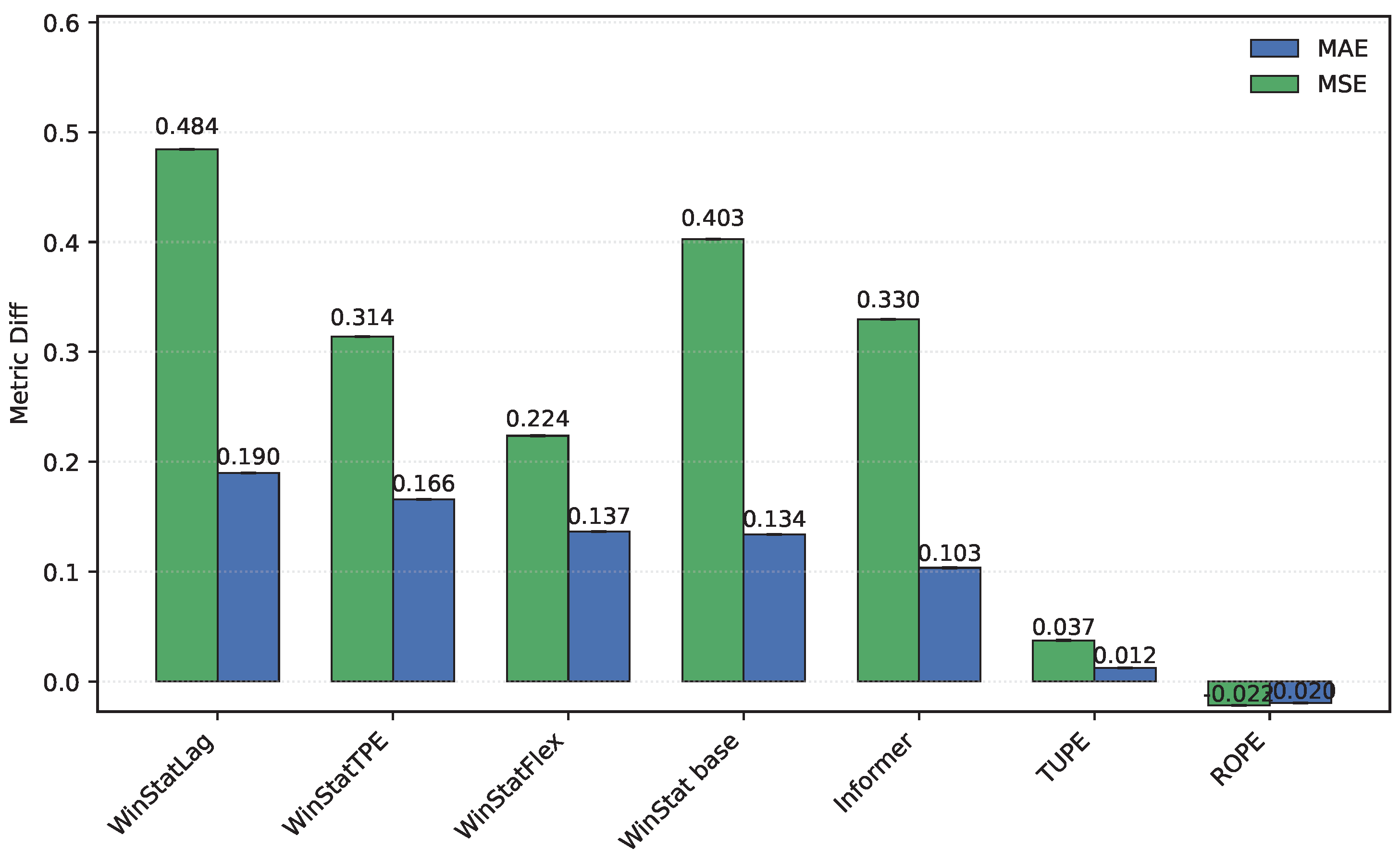
Figure 10.
Comparison of original and shuffled models on the ETTh2 dataset. Higher values show more effective use of semantic and ordering information. A larger gap indicates higher ordinal dependence of the encoding, disrupted by shuffling.
Figure 10.
Comparison of original and shuffled models on the ETTh2 dataset. Higher values show more effective use of semantic and ordering information. A larger gap indicates higher ordinal dependence of the encoding, disrupted by shuffling.
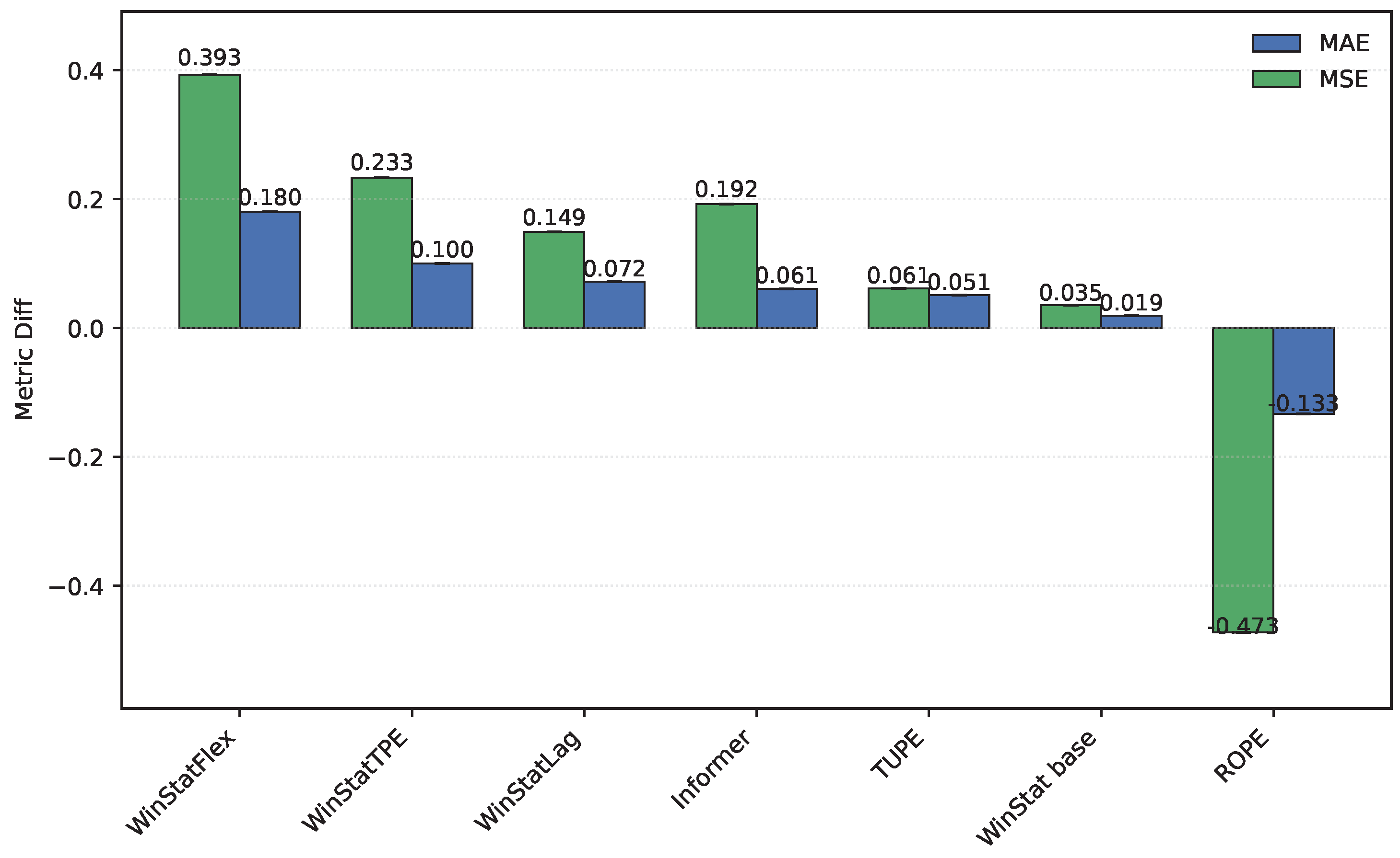
Figure 11.
Comparison of original and shuffled models on the NYC dataset ((MAE on top, MSE on bottom, separated due to significantly different scales)). Higher values denote stronger integration of semantic and ordering information. Greater differences imply stronger ordinal dependence in the encoding, which is lost when data are shuffled.
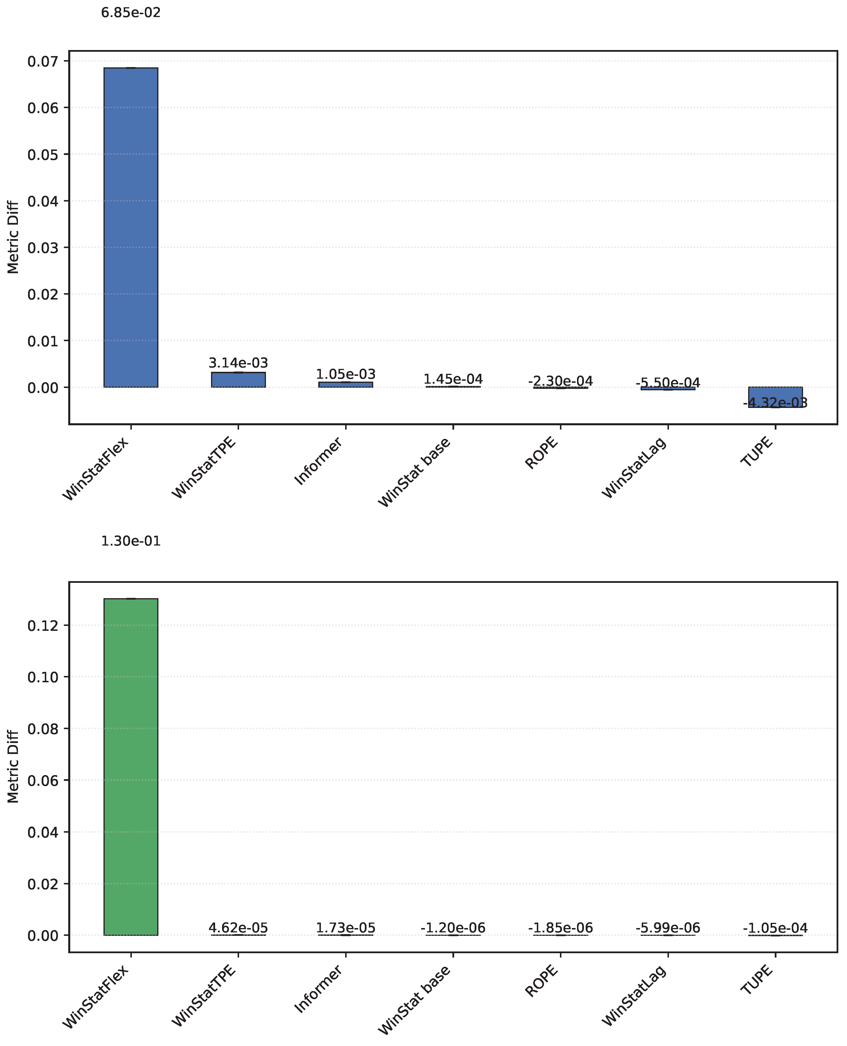
Figure 12.
Comparison of original and shuffled models on the TINA dataset. Higher values indicate better incorporation of semantic and ordering information. A larger difference points to greater ordinal dependence of the encoding, which is broken by shuffling.
Figure 12.
Comparison of original and shuffled models on the TINA dataset. Higher values indicate better incorporation of semantic and ordering information. A larger difference points to greater ordinal dependence of the encoding, which is broken by shuffling.
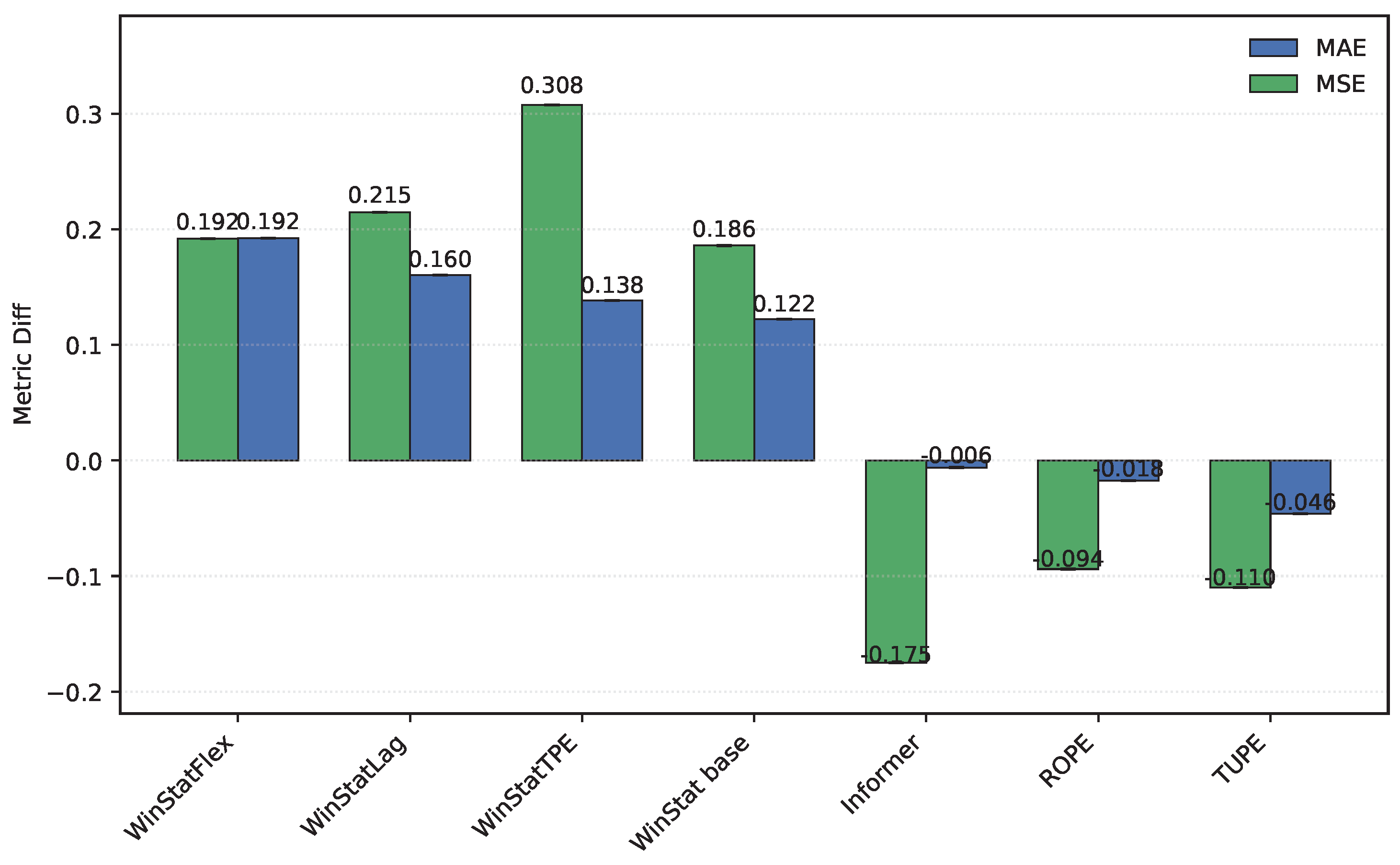
Table 1.
Summary of positional encoding approaches in Transformer-based time series models.
| Method | Type | Injection | Attributes |
|---|---|---|---|
| Absolute Positional Encoding (APE) [19] | Absolute, Fixed | Additive to embeddings | Parameter-free, extrapolates to unseen lengths, based on functions. |
| Learnable PE (LPE) [14] | Absolute, Learnable | Additive to embeddings | Trainable parameters per position; flexible but lacks extrapolation. |
| time Absolute PE (tAPE) [7] | Absolute, Fixed | Additive to embeddings | Rescales sinusoidal frequencies using sequence length L to preserve distance-awareness. |
| Relative PE (RPE) [13] | Relative, Learnable | Modifies attention scores | Encodes pairwise offsets in attention weights; translation invariant but memory heavy. |
| efficient RPE (eRPE) [7] | Relative, Learnable | Modifies attention scores | Memory-efficient relative PE variant; scalable to long sequences. |
| TUPE [28] | Hybrid (Abs+Rel), Learnable | Attention-level | Untied projections for query, key, and position embeddings; richer interactions between content and position. |
| RoPE [29] | Relative, Fixed | Rotation in embedding space | Encodes positions via complex rotations; preserves relative distances multiplicatively. |
| Temporal PE (T-PE) [8] | Hybrid (Abs+Semantic) | Additive + attention-level | Combines sinusoidal encoding with a Gaussian similarity kernel over inputs; couples global periodicity and local semantics. |
| Representative / Global Attention [30] | Relative, Fixed | Modifies attention scores | Variants tailored for anomaly detection and TSF: Representative focuses on local lags, Global captures long-range dependencies. |
Table 2.
Common hyperparameters per dataset used across all positional-encoding variants. All runs use full (vanilla) self-attention to isolate the effect of positional encoding.
Table 2.
Common hyperparameters per dataset used across all positional-encoding variants. All runs use full (vanilla) self-attention to isolate the effect of positional encoding.
| Dataset | Attention | Batch | Dropout | Runs | w | L | Label | Pred |
|---|---|---|---|---|---|---|---|---|
| HPC (UCI) | Vanilla | 32 | 0.2 | 3 | 60 | 180 | 60 | 60 |
| ETT (ETTh1/ETTh2) | Vanilla | 32 | 0.2 | 5 | 24 | 96 | 48 | 24 |
| Yellow Trip (NYC) | Vanilla | 32 | 0.2 | 3 | 60 | 180 | 60 | 60 |
| TINA (Industrial) | Vanilla | 32 | 0.2 | 3 | 288 | 96 | 48 |
† On TINA, the window w was capped by GPU memory constraints even though the ETT pilot study suggested w ∈ [L/4, L/3].
Table 3.
Comparison of the WinStat family across five datasets (vs. Informer, sinusoidal, no PE, ROPE, and TUPE). Values represent the mean ± standard deviation over three runs. Bold values indicate the best results for each dataset and metric.
Table 3.
Comparison of the WinStat family across five datasets (vs. Informer, sinusoidal, no PE, ROPE, and TUPE). Values represent the mean ± standard deviation over three runs. Bold values indicate the best results for each dataset and metric.
| Encoding | Metric | HPC | ETTh1 | ETTh2 | Yellow Trip | TINA |
|---|---|---|---|---|---|---|
| Informer | MAE | |||||
| MSE | ||||||
| PE (sin/cos) | MAE | |||||
| MSE | ||||||
| WinStat base | MAE | |||||
| MSE | ||||||
| WinStatLag | MAE | |||||
| MSE | ||||||
| WinStatFlex | MAE | |||||
| MSE | ||||||
| WinStatTPE | MAE | |||||
| MSE | ||||||
| TUPE | MAE | |||||
| MSE | ||||||
| ROPE | MAE | |||||
| MSE | ||||||
| No PE | MAE | |||||
| MSE |
Table 4.
HPC: learned mixture weights in WinStat variants (normalized). The symbol * identifies a component not considered in the weighting definition
Table 4.
HPC: learned mixture weights in WinStat variants (normalized). The symbol * identifies a component not considered in the weighting definition
| Component | WinStatFlex | WinStatTPE |
|---|---|---|
| Stats | ||
| PE | ||
| LPE | ||
| tAPE | * | |
| TPE | * |
Table 5.
ETTh1: learned mixture weights in WinStat variants (normalized). The symbol * identifies a component not considered in the weighting definition.
Table 5.
ETTh1: learned mixture weights in WinStat variants (normalized). The symbol * identifies a component not considered in the weighting definition.
| Component | WinStatFlex | WinStatTPE |
|---|---|---|
| Stats | 0.2704 | 0.2580 |
| PE | 0.2506 | 0.2470 |
| LPE | 0.2420 | 0,2320 |
| tAPE | 0.2371 | * |
| TPE | * | 0.2630 |
Table 6.
ETTh2: learned mixture weights in WinStat variants (normalized). The symbol * identifies a component not considered in the weighting definition.
Table 6.
ETTh2: learned mixture weights in WinStat variants (normalized). The symbol * identifies a component not considered in the weighting definition.
| Component | WinStatFlex | WinStatTPE |
|---|---|---|
| Stats | 0.2569 | 0.2510 |
| PE | 0.2504 | 0.2490 |
| LPE | 0.2513 | 0.2490 |
| tAPE | 0.2413 | * |
| TPE | * | 0.2510 |
Table 7.
NYC: learned mixture weights (normalized).The symbol * identifies a component not considered in the weighting definition.
Table 7.
NYC: learned mixture weights (normalized).The symbol * identifies a component not considered in the weighting definition.
| Component | WinStatFlex | WinStatTPE |
|---|---|---|
| Stats | ||
| PE | ||
| LPE | ||
| tAPE | * | |
| TPE | * |
Table 9.
Comparison of differences between shuffled and original encodings on 5 datasets. Values are the mean differences (Shuf − Orig) over 3 runs.
Table 9.
Comparison of differences between shuffled and original encodings on 5 datasets. Values are the mean differences (Shuf − Orig) over 3 runs.
| Encoding | Metric | HPC | ETTh1 | ETTh2 | NYC | TINA |
|---|---|---|---|---|---|---|
| Informer (Shuf.) | MAE | 0.0047 | 0.1035 | 0.0608 | -0.0061 | |
| MSE | 0.0155 | 0.3297 | 0.1924 | -0.1751 | ||
| WinStat base (Shuf.) | MAE | 0.1043 | 0.1423 | 0.0173 | 0.1225 | |
| MSE | 0.1952 | 0.4235 | 0.0170 | 0.1860 | ||
| WinStatLag (Shuf.) | MAE | 0.2072 | 0.2125 | 0.1059 | 0.1603 | |
| MSE | 0.4946 | 0.5444 | 0.2477 | 0.2148 | ||
| WinStatFlex (Shuf.) | MAE | 0.2077 | 0.1366 | 0.1800 | 0.1924 | |
| MSE | 0.3202 | 0.2237 | 0.3932 | 0.1919 | ||
| WinStatTPE (Shuf.) | MAE | 0.2067 | 0.1657 | 0.1003 | 0.1385 | |
| MSE | 0.3875 | 0.3139 | 0.2330 | 0.3076 | ||
| ROPE (Shuf.) | MAE | 0.0181 | -0.0195 | -0.1334 | -0.0176 | |
| MSE | 0.0169 | -0.0218 | -0.4728 | -0.0939 | ||
| TUPE (Shuf.) | MAE | 0.0129 | 0.0124 | 0.0512 | -0.04600 | |
| MSE | 0.0121 | 0.0374 | 0.0613 | -0.1098 |
Disclaimer/Publisher’s Note: The statements, opinions and data contained in all publications are solely those of the individual author(s) and contributor(s) and not of MDPI and/or the editor(s). MDPI and/or the editor(s) disclaim responsibility for any injury to people or property resulting from any ideas, methods, instructions or products referred to in the content. |
© 2025 by the authors. Licensee MDPI, Basel, Switzerland. This article is an open access article distributed under the terms and conditions of the Creative Commons Attribution (CC BY) license (http://creativecommons.org/licenses/by/4.0/).
Copyright: This open access article is published under a Creative Commons CC BY 4.0 license, which permit the free download, distribution, and reuse, provided that the author and preprint are cited in any reuse.


