Submitted:
03 November 2025
Posted:
04 November 2025
You are already at the latest version
Abstract
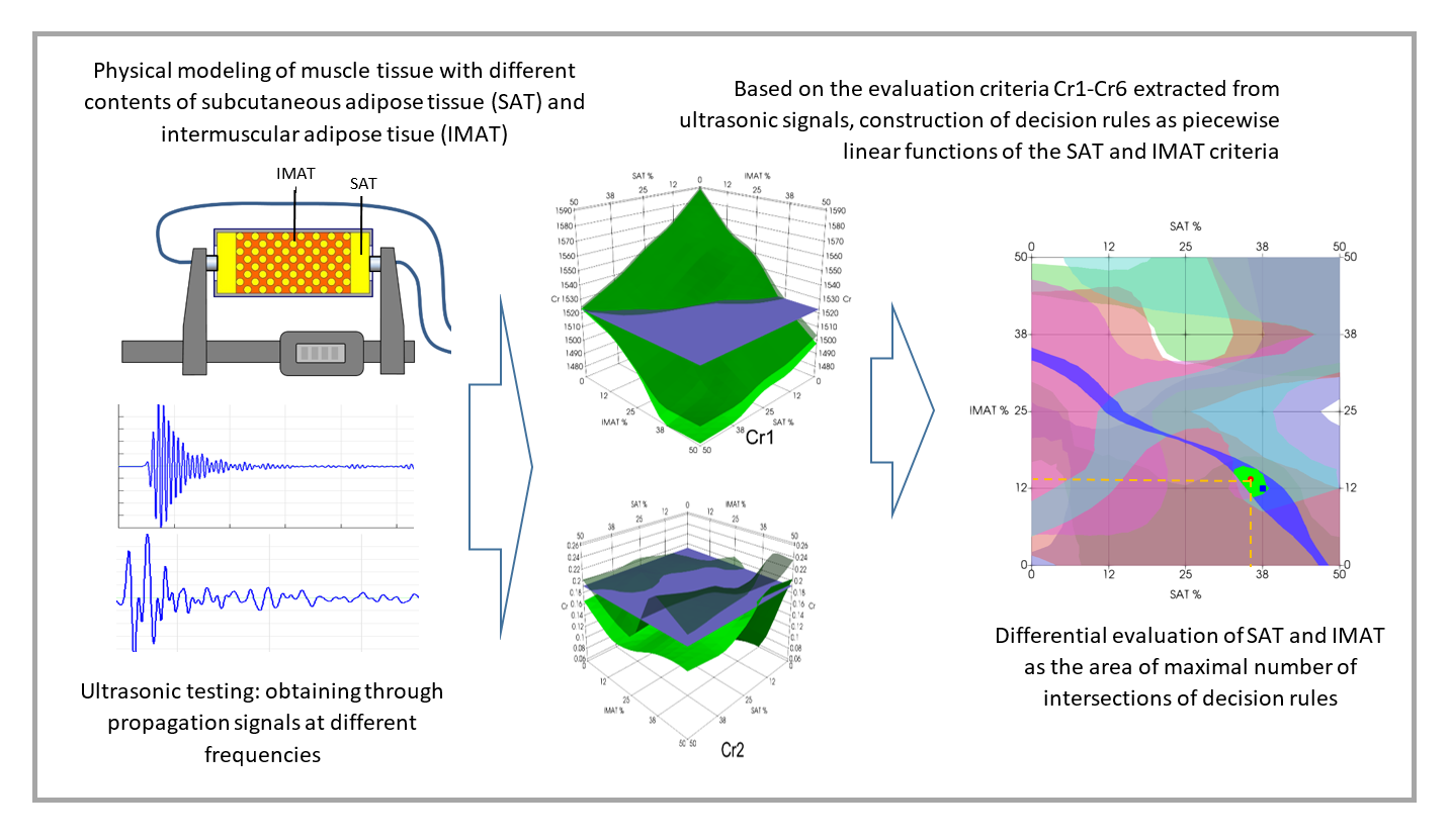
In medical diagnostics, there are strong reasons to distinguish between subcutaneous adipose tissue (SAT) and intermuscular adipose tissue (IMAT), as infiltration of IMAT into muscle causes health complications with aging (sarcopenia), diabetes, cardiovascular disease, and obesity. Since such assessments are performed using stationary and labor-intensive imaging modalities (MRI, CT), the development of portable devices based on ultrasound measurements, could aid proactive medicine and expand screening capabilities. The aim of this model study was to demonstrate the feasibility of differentially assessing SAT and IMAT by extracting evaluation criteria from propagating ultrasound signals. A set of 25 phantoms, using gelatin gel as the muscle matrix and oil for the SAT and IMAT compartments, formed a network with gradual changes in SAT and IMAT ranging from zero to 50%. Ultrasound signals were recorded at frequencies of 0.8 and 2.2 MHz, and assessment criteria were used, including ultrasound velocity and intensity derivatives. The intersection of decision rules based on evaluation criteria generated domains of possible recognition solutions. In parallel, using the same data partitions for training and test sets, artificial neural network (ANN/LSTM) analysis was applied. Both approaches demonstrated diagnostically acceptable SAT and IMAT resolution, opening up prospects for the ultrasound method.
Keywords:
intermuscular and subcutaneous adipose tissues
; ultrasonic measurements
; pattern recognition
; artificial neural networks
; tissue models
1. Introduction
Subcutaneous adipose tissue (SAT) and intermuscular adipose tissue (IMAT) are two distinct forms of fat depots in human limbs with markedly different biological, functional, and clinical implications. SAT is the most widely distributed subcutaneous fat tissue layer composed of adipocytes found just beneath the skin that surrounds muscles externally. IMAT is fatty infiltration between and within muscle groups located in the perimuscular and intermuscular compartments and referring to storage of lipids in adipocytes underneath the deep fascia of muscle. This includes the visible storage of lipids in adipocytes located between the muscle fibers and between muscle groups [1]. Although both depots contribute to whole-body adiposity, their physiology and pathological significance diverge substantially.
While total adiposity is a strong predictor of cardio-metabolic risk, differentiating SAT from IMAT is critical for musculoskeletal, metabolic and geriatric medicine. Excess SAT in the limbs reflects energy storage but does not directly impair muscle contractility. By contrast, IMAT compromises muscle strength per unit area, reduces insulin sensitivity, and exacerbates mobility decline [2,3]. Clinical studies demonstrate that IMAT, not SAT, is the stronger predictor of falls, frailty, and impaired rehabilitation outcomes after orthopedic surgery [4,5]. Thus, precise assessment of both compartments allows improved stratification of osteosarcopenia, sarcopenic obesity, diabetes, and neuromuscular disorders.
SAT thickness in the human lower limbs (thigh and calf) is typically in the range of about 4–20 mm depending on sex, body mass index (BMI) and location (anterior thigh often thicker than lateral thigh/calf) [6]. Measurements by different techniques show large inter-subject variability. In thigh and calf regions of normal-weight adults SAT varies in the range 4–12 mm, while in overweight and obese subjects it can reach 40 mm and more [7]. Volumetric IMAT values reported as a percentage of muscle compartment vary in thigh muscles in normal-to-pathological cohorts range from about 1% to >30–35%. [8].
There are several clinical and pathophysiological reasons for differential evaluation of SAT and IMAT. In the sense of metabolic consequences, IMAT is strongly associated with insulin resistance, type-2 diabetes and systemic metabolic dysfunction even after controlling for total fat. IMAT and intramyocellular lipid correlate with impaired glucose uptake and local inflammatory signaling [9]. SAT, by contrast, is metabolically “safer” in many contexts. In older adults, an elevated IMAT infiltration correlates with reduced strength, poorer mobility, worse surgical outcomes and higher frailty associated with sarcopenia, myosteatosis and sarcopenic obesity [4,10]. Differential measurement helps identify sarcopenic obesity and stratify patients into risk groups. Infiltration of fat within and between muscles known as myosteatosis alters muscle quality resulting in the local mechanical and functional impact, and specifically in contractile efficiency, promoting fibrosis [11]. Therefore, IMAT estimation is relevant for rehabilitation and orthopedic planning. Knowledge of IMAT separately from SAT in disease-specific implications, including, in obesity, type-2 diabetes mellitus, chronic kidney disease, chronic inflammatory states and muscle atrophy after disuse and immobilization helps understanding disease mechanisms and target interventions. It is taken into account that exercise reduces IMAT preferentially [8]. Some studies revealed independent association of IMAT deposit in the thigh with cardiometabolic risk factors (including total blood cholesterol, low-density lipoprotein (LDL), and triglycerides), and decreased insulin sensitivity. The SAT/IMAT ratio is associated with serum adiponectin levels and this factor could possibly serve as an indicator for individual factors of a person´s cardiovascular risk [12].
Figure 1 schematically shows cross-sections of a hypothetical human limb, demonstrating various SAT and IMAT ratios under different conditions, based on a series of literary sources [13,14,15,16] that provide corresponding tomographic images. In a healthy normal-weight human limb, SAT typically constitutes the predominant fat compartment, while IMAT is minimal, resulting in a high SAT-to-IMAT ratio (I). In a type-2 diabetes patient with significant IMAT infiltration, the SAT-to-IMAT ratio is reduced due to a relative increase in IMAT with normal or even reduced SAT, reflecting abnormal fat redistribution within the limb (II). During the progression of obesity, SAT initially expands predominantly, maintaining a high SAT-to-IMAT ratio, but with advancing obesity and metabolic dysfunction, IMAT gradually increases, leading to a decline in the SAT-to-IMAT ratio as fat increasingly infiltrates muscle compartments (III-IV).
Non-invasive techniques for measuring SAT and IMAT in human limbs are based on accurate, depot-specific quantification that require imaging and either a tissue-specific signal (magnetic resonance imaging, proton-density fat fraction (MRI PDFF)) or an attenuation signature (computed tomography — Hu-based segmentation (CT HU)) or validated surrogate (ultrasonography). MRI PDFF directly estimates fat fraction and can biochemically separate intra- and extramyocellular lipids in a localized voxel. Possessing a high soft-tissue contrast, volumetric PDFF maps permit fascia-aware segmentation to separate SAT and IMAT and enable longitudinal quantification [16,17,18]. Due to such limitations as cost, scanner access and stationarity, MRI use is restricted to research where precise depot separation and quantitative tracking are required. In CT HU-based segmentation, anatomical cross-sectional areas and volumes differencing by radiological density are measured [19]. Fat is identified by low Hounsfield units, where 190 HU is typical for fat and 30 HU for muscle. The advantage of CT is the possibility to quantify the muscle density also termed as muscle attenuation or muscle radiation attenuation, which linearly depends on the muscle fat content [20]. High spatial resolution of CT allows retrospective opportunistic analysis from clinical CTs, however, limited by its ionizing radiation, stationarity and availability. Ultrasonography or clinical ultrasound, exploring the association between skeletal muscle echogenicity and its physical properties presents an opportunity to be utilized as a screening tool [6,21]. Mostly, it suggests quantification of SAT thickness; however, the prediction of IMAT is still problematic despite muscle echo intensity and texture are revealed as surrogate markers for muscle fat.
There is a sound physical and physiological rationale for exploring single-channel through-transmission ultrasound to estimate SAT and IMAT separately, although the method is still experimental and faces some practical challenges. The physical basis for this is a strong dependence of acoustic properties of tissues on fat content [22,23,24]. Acoustic impedance, ultrasound velocity (speed of sound) and attenuation systematically differ between lean and adipose tissues. The speed of sound in lean muscle tissue ranges from 1540 to 1580 m/s, while in adipose tissue it is from 1440 to 1480 m/s. The attenuation ranges are 0.3 to 0.7 dB/cm·MHz in lean tissue and 0.6–1.0 dB/cm·MHz in adipose tissue, respectively. Thus, the systematic accumulation of fat in tissue should exhibit a linearly decreasing trend for sound velocity and an increasing trend for attenuation [25]. These differences produce layer-specific acoustic signatures in through-transmission measurements and cause characteristic refraction, attenuation, and frequency dispersion, which in principle can be inverted to estimate the thickness and composition of the layers. By analyzing the through-transmitted signal in broadband frequency, the arrival time and phase velocity can estimate an apparent bulk velocity, amplitude decay and spectral slope can give attenuation, and inversion with a layered model can estimate SAT thickness (layer 1) and IMAT-induced changes in layer 2 (muscle). Such inversion is analogous to geophysical layer property estimation or ultrasonic bone thickness/porosity inversion [26]. If such a quantitative ultrasound solution is implemented, it has the potential to become an inexpensive and portable alternative to MRI and CT.
The aim of the study was to demonstrate the potential for differential assessment of SAT and IMAT in simple muscle models by applying pattern recognition methods and neural network analysis to the data derived from ultrasound signals in through transmission. Similar approaches of pattern recognition applications for the evaluation of factors-of-interest based on ultrasonic parameters as decision rules have been developed previously for different physical objects and corresponding testing tasks. For example, the possibility of determining the depth and the degree of deterioration of the surface layer of concrete by the combined use of ultrasonic surface waves at different frequencies was proven implementing a mathematical approach of pattern recognition using statistical criteria and neural networks [27,28]. The universality of this approach was shown for testing different materials with differentiation of factors-of-interest [29,30]. The estimation method for cortical thickness and intracortical porosity in compact bone models of osteoporosis as the two factors of bone quality used either statistical characteristics of ultrasonic signals or physical parameters of ultrasound propagation extracted from spatiotemporal waveform profiles [31,32].
2. Materials and Methods
2.1. Muscle Mimicking Phantoms with SAT and IMAT Variation
Ultrasound tissue phantoms were designed to simulate the combined effects of SAT and IMAT in a conditional muscle in the ranges close to physiological ones attributed to different physiological conditions. The phantom shown in Figure 2 represented a 3D printed plastic 80x40x30 mm mold with fixed grooves for placing acoustically transparent partitions separating SAT sections. On the opposite edges of the long side, there were windows covered with acoustically transparent membranes for the attachment of ultrasonic transducers for through transmission sounding of the phantom. Symmetric sections of the SAT were located at the opposite edges of the phantom, and “muscle tissue” section with simulated IMAT inclusions was located in the middle. The SAT content was varied by the thickness of symmetrical SAT sections at the edges, and the IMAT content was varied by 5 mm diameter cylindrical inclusions inserted in a staggered pattern in the central "muscular" region. The IMAT inclusions (holes) were made using specially printed inclusion-setting dies (Figure 3).
Since the ultrasonic measurements in the experiment were carried out at room temperatures (21-23ºC), the materials for simulating the muscle tissue matrix and adipose tissue (SAT and IMAT) were selected in such a way to correspond approximately (at room temperature) the acoustic properties of lean muscle and fat at the temperature in the human body (about 37 ºC). The muscle tissue matrix was mimicked by a stiffened water solution of 20% of animal gelatin. This gelatin-based gel has ultrasound velocities in the range of 1570-1580 m/s at room temperature [33] that is close to the ultrasound velocities in non-obese human muscle in vivo [34]. The fat content for both SAT and IMAT inclusions was mimicked by extra-virgin olive oil where ultrasound velocity was reported as 1453 ± 2 m/s at room temperature [35] is also a very close match 1450 m/s typically for human adipose fa) at 37 °C [24,36]. The anisotropy of acoustic properties the presence and orientation of muscle fibers in real muscles was not taken into account in our case. Both SAT and IMAT contents were gradually varied from zero to 50 % with a step 12.5%. In this case, the SAT gradations were determined by the thickness of the SAT layer in relation to the entire volume of the phantom (Figure 2), and the IMAT gradations were related to the remaining part of the “muscle” component or gelatin matrix denoted by the concentration of inner holes (Figure 3). The set included a net of 25 phantoms with five grades of SAT and five grades of IMAT that varied independently presenting 25 possible combinations of SAT and IMAT.
2.2. Ultrasonic Measurements
Ultrasonic signals were obtained by testing the phantom in through transmission mode using a pair of transmitting and receiving transducers stiffly mounted on opposite arms of a digital caliper in such a way as to ensure parallelism and centering of the transducers. The experimental setup is shown in Figure 4. The acquisition of ultrasonic signals was controlled by a custom circuit based on an Altera Cyclone IV EP4CE22E22C8 field programmable logic array (FPGA) chip, interacting with the exchange of commands and data with the computer via a USB 3.0 interface chip FIFO FT600Q. The FPGA controlled the output amplifier - a high-voltage pulsar HV7360 from Microchip, providing the emission of ultrasonic tone pulses with an output voltage of up to 200 V peak-to-peak. The received ultrasonic signals were passed through an Analogue Devices AD8367ARUZ voltage gain amplifier (VGA) with a voltage gain of up to 45 dB and digitized by the LTC2250 ADC, a 10-bit, low-noise, 125Msps/105Msps Linear Technology ADC designed for digitizing high-frequency signals with a wide dynamic range. The high and low voltages in the circuit were provided by an Analogue Devices LT8331 DC/DC converter. The FPGA processing core managed the transmission and receiving data streams in FIFO buffer memory registers and additional buffers for digitized received signals and transmitted waveforms.
The ultrasonic signals were obtained as a signal train containing three separate waveforms per pass: excitation at a carrier frequencies of 0.8 MHz and 2.2 MHz, and a frequency sweep in the range from 0.5 to 2.5 MHz. The sequence of received direct propagation signals, their expanded fragments and the corresponding spectra after FFT processing are presented in Figure 5. The frequencies of 0.8 and 2.2. MHz were the resonant frequencies of the disk-type transducers used, and the excitation waveforms were tone-busts of two period sinusoids of these frequencies enveloped by a sine half-period. The sweep waveform contained both low frequency (below 1 MHz) and high frequency (around 2 MHz) components. The sweep waveform was strong enough to record the second reflection, i.e. the ultrasonic signal that passed through the phantom three times, which was also used in further data processing.
Each phantom was measured 15 times that resulted in 375 individual signal sets (signal trains). The acoustic base was simultaneously measured with a digital caliper with an accuracy of 0.1 mm.
2.3. Determination of Ultrasonic Parameters as Evaluation Criteria for Pattern Recognition and Neural Network Analysis
After considering a number of physical parameters of wave propagation in phantoms, their variability, and sensitivity to the factors of interest – SAT and IMAT, the evaluation criteria (Cr) were selected. These included ultrasound velocity and parameters related to changes in signal intensity as they passed through the phantom at different frequencies (direct propagation and third passing).
Finally, six criteria were selected, each with different trends and quantitative indicators of dependence on SAT and IMAT:
Cr1 – ultrasound velocity. Ultrasound velocity C (m/s) was calculated as
where L is distance between emitter and receiver, t is ultrasound arrival time measured by the first zero-crossing as the signal reference point, Δt is the transducers constant at zero distance;
C = L/(t-Δt),
Cr2 and Cr3 – ultrasound attenuation at frequencies 0.8 and 2.2 MHz, α0.8MHz and α2.2MHz correspondingly;
Ultrasound attenuation at a certain frequency α (dB/cm) was calculated as
where I0 is the signal intensity or the integral of the signal amplitudes at zero distance, I1 is the same at distance L. The integrals I were calculated as sum of amplitude values Sn in the corresponding time windows:
where ns is start index, ne is end index, n –is the number of signal discretization points;
α =(20log(I0/I1))/L ,
Cr4 –ratio of attenuation values at 0.8 and 2.2 MHz, determined as α0.8MHz/ α2.2MHz;
Cr5 – intensity of sweep signal determined as the integral of signal amplitudes in the fixed-length time window;
Cr6 – The ratio of signal intensities between the sweep signal in direct pass and its second reflection (triple pass through the phantom) (Figure 5).
2.4. Methodology of Recognition and Data Structure
The evaluation of the IMAT and SAT as factors-of-interest in the objects (phantoms) was based on the analysis of the initial data, as well as on the principles of pattern recognition and artificial neural networks. The methodology consisted of three main stages:
- constructing and analyzing patterns of evaluation criterion (Cr) values depending on IMAT and SAT values;
- using pattern recognition methods to analyze IMAT and SAT values. These methods are based on constructing and applying decision rules based on a training dataset and then applying these rules to analyze the test object.
- using artificial neural networks to analyze IMAT and SAT values. This approach is also based on the use of training and test datasets and the application of ANN to analyze the test object.
The structure of the source data used in this work is an orthogonal grid of objects with uniform gradations of IMAT and SAT values ranging from 0% to 50% with a step of 12.5% (Figure 6).
Each object was described by a set of 15 complex signals, or signal trains, illustrated in Figure 6, which were repeated measurements with the transducers removed and acoustic contact restored. From each of these signals, six evaluation criteria Cr1 - Cr6 for two variable factors-of-interests, SAT and IMAT, were calculated. For a single signal, the record structure was as follows:
| Signal number | IMAT | SAT| Cr1| Cr2 | Cr3 | Cr4 | Cr5 | Cr6|.
2.5. Recognition Based on Pattern Recognition Using Decision Rules
After calculating the evaluation criteria Cp1-Cr6 for each signal, the maximum and minimum values of each criterion were determined for each object. These values were used to construct a three-dimensional volume, where the upper boundary surface is a piecewise linear interpolation function with the maximum parameter value, and the lower boundary surface is a piecewise linear interpolation function with the minimum parameter value. Then, to increase the number of data points in this volume, the upper and lower surfaces were interpolated using Akima interpolation splines, and three new interpolated points were added between each real data point. This increased the number of points from 5 to 17 on each axis.
To evaluate a new object with unknown SAT and IMAT values, the same evaluation criteria Cr1 – Cr6 were calculated from the received signal train. The intersection region between each calculated criterion and the volume of the same criterion determined from the training series was then constructed, which could yield one or more intersection areas. This intersection region represented a set of possible answers for SAT and IMAT values in two-dimensional space. To obtain the final answer, the intersection of all six areas upon all evaluation criteria was determined. To localize the final answer, it was determined as the center of mass of the intersection figure with the corresponding coordinates in the SAT-IMAT scale. The recognition procedure is illustrated in Figure 7.
2.6. Recognition Based on Artificial Neural Network
The Long Short-Term Memory (LSTM) method was used as the main method in the experiment. LSTM is a specialized Recurrent Neural Network (RNN) architecture designed for processing and analyzing data with long-term temporal dependencies. It addresses classical RNN issues, such as vanishing and exploding gradients, ensuring reliable learning from sequential data. This is achieved through a unique structure that includes memory cells and three main types of gates: the forget gate, input gate, and output gate. The structure of LSTM cell is illustrated in Figure 8, where: Xt– current input data fed into LSTM cell; ht– hidden state; Ct– cell state; ht-1– hidden state from the previous time step, containing information about past data; Ct-1– cell state at the previous time step, storing long-term information; it– input gate;
The model utilized a hyperbolic tangent function (tanh). The hyperbolic tangent function is a commonly used activation function in LSTM networks. This function maps input values in range [-1, 1], making it useful for regulating flow of information within the network.
where x is input value; e is Euler’s number.
Tanh is zero-centered, allowing both positive and negative activation. This property helps in preserving balance of information during training, reducing bias accumulation.
Validation loss (val_loss) key metric were used to evaluate the performance of LSTM model during training. This metric represents the error calculated on validation dataset, which consists of data that model has not seen during training. Validation loss is computed using the same loss function as the training loss (Mean Squared Error).
Mean Squared Error (MSE) measures average squared difference between the predicted values and actual target values.
where: N is total number of samples; is actual value of i-th sample; is predicted value for i-th sample.
Since error is squared, MSE penalizes larger deviations more heavily than smaller ones making it sensitive to outliers. A lower MSE indicates better model performance, as it means predictions are closer to the true value.
R squared score is a statistical metric used to evaluate performance of regression models. It measures how well model’s predictions approximate actual values by comparing explained variance to the total variance in data.
where: – actual value of i-th sample; – predicted value of i-th sample; – mean of all actual values; N – total number of samples.
R squared score ranges from -∞ to 1. High R squared score indicates that model better explains variance in target variable. However, high R squared score does not mean accurate predictions.
3. Results and Discussion
3.1. Experimental Decision Rules
The three-dimensional images of the decision rules, constructed in accordance with the mathematical criteria Cr1 – Cr6 (Figure 9) as piecewise linear functions of SAT and IMAT, visualize the multidirectional changes in the decision rules for these criteria in SAT-IMAT coordinates. The complex appearance of the graphs reflects the complex influence of SAT and IMAT on these criteria, which is observed in the form of multidirectional trends and the presence of local extremes in different areas of the SAT-IMAT space. The exception is the decision rule for Cr1 (Figure 9a) that is ultrasound velocity, which shows a linear monotonic decrease along both the SAT and IMAT axes, resulting in a smooth slope of the Cr1 surface, close to a linear plane. The character of the decision rules according to the Cr2-Cr6 criteria is difficult to interpret physically without the use of physical and mathematical simulations of the mutual influence of SAT and IMAT on ultrasonic attenuation. Since an increase in IMAT introduces a scattering effect and causes attenuation of the forward ultrasound propagation (while the echogenicity of the B-mode signal demonstrated a growth [21]), the appearance of two homogeneous SAT layers against this background weakens this effect. In general, trends towards increasing ultrasound attenuation (Cr2, Cr,3, Cr,5) and the frequency slope of attenuation (Cr4) with increasiung SAT and IMAT, especially with increasing IMAT due to scattering, and, consequently towards decreasing the ratio of the direct signal propagation to its third pass after double reflection (Cr6) were observed. This conclusion, obtained on tissue phantoms, coincides with the general idea that ultrasound attenuation in lean muscle is approximately half that in fat [23,24]. However, the combined effect of different ratios of homogeneous fat (SAT) and dispersed fat (IMAT) makes these relationships quite complex that is reflected in the complicated shapes of the decision rules for Cr2-Cr6. Moreover, the interface between the SAT layers and the hypothetical muscle containing IMAT inclusions makes its own reflexive contribution. Since the study did not aim to analyze in detail the physical causes of the complex SAT-IMAT effects, the experimental data were accepted as phenomenological, as they were obtained during the experiment.
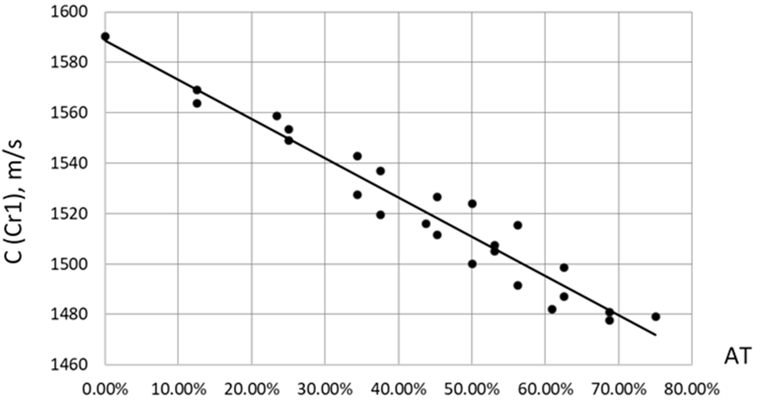
As for ultrasound velocity (the first evaluation criterion Cr1), when constructing the correlation of the velocity C from the total content of adipose tissue AT= SAT + IMAT (%), a clear linear dependence of the form C = 1589 - 155.9*AT (m/s) was discovered. The Pearson linear correlation coefficient was P = -0.97. In this case, AT varied from zero to 75% at maximum SAT = 50% and IMAT = 50%, since SAT was set from the entire volume of the phantom, and IMAT only from its “muscle” component. The C slope vs. AT content was decline of C to 1.57 m/s with AT increase on 1%. This finding remarkable coincide with the similar results obtained for ultrasound velocity in human lower limb muscle depending on fat content [37,38].
Figure 10.
Empirical correlations between ultrasound velocity C and total fat content AT = SAT + IMAT in muscle phantoms.
Figure 10.
Empirical correlations between ultrasound velocity C and total fat content AT = SAT + IMAT in muscle phantoms.
To assess how much the measurement of each criterion varies between objects compared to how much it varies within an object, and to express the degree of discrimination between objects, individuality indices (II) and the reciprocals of the II (RII) were calculated. These and other statistical input data for this assessment are presented in Table 1. As generally it is accepted [39,40], a parameter shows low individuality or poor discrimination at an II < 0.6; i.e. population-based reference intervals are useless. Otherwise, at an II > 1.4, the parameter exhibits high individuality, and individual values vary substantially between objects. Conversely, a higher RII is an index of heterogeneity and an indicator of a stronger discriminatory power between objects [39,41]. The obtained data showed the highest RII for Cr1 - ultrasound velocity – which many times higher than that for other criteria. In this sense, this indicates a multiple discriminatory power of ultrasound velocity compared to other criteria based on measurements of ultrasound signal intensity. Thus, the Cr1 criterion should be considered the primary criterion reflecting the combined influence of SAT and IMAT, where other criteria have a clarifying function for discrimination between SAT and IMAT. Since each of these criteria Cr2- Cr6 has higher individuality or lower discriminative power relative to Cr1, their combined use and more overlapping criteria may help to better resolve of SAT and IMAT.
3.2. Evaluation Experiment
In this study, the effectiveness of the proposed evaluation methods was tested experimentally. For this purpose, the scan data was split by five different ways.
In Splits 1–3, the data was divided by index, meaning three signals with identical indices from the total number of 15 signals (repeated measurements with contact recovery) in each of 25 objects were used for testing. In Splits 4–5, three randomly selected signals from each object were used for the test set, and the remaining signals were used for the training set.
The obtained database was used to conduct five similar experiments. Each experiment utilized the corresponding signal split, a decision rule approach, and an artificial neural network (LSTM).
3.3. Recognition Results
Figure 11 demonstrates the results of experimental estimation of IMAT and SAT in a few test objects using the proposed decision rules approach. These examples are chosen to show cases of varying degrees of estimation accuracy. The estimation result (the green segment of intersection of all six decision rules centered on the red dot) in general show diagnostically appropriate accuracy of estimation as compared to a-priori known projected values of the test object (blue point). As Figure 11 shows, the estimation result in the majority cases was accurate within the accuracy of the phantoms fabrication (A – D). However, decision rules could produce multiple intersection segments, leading to multiple possible answers (E, F). In these cases, the average value of all possible answers can be found; however, it generally does not provide the exact match with the projected value. Furthermore, when using a decision rule-based approach, a situation may arise where some decision rules in the experiment do not intersect or fall outside the recognition area, resulting in no segment being formed. Examples (G, H) demonstrate such cases. In this case, the decision segment is obtained using the intersection of fewer than six segments.
3.4. Artificial Neural Network Analysis
The neural network experiments were performed using the same dataset and data partitions as in the pattern recognition experiments, ensuring consistency of training and testing conditions. For each of the five data splits, the LSTM network was trained independently to estimate the IMAT and SAT parameters from the corresponding ultrasound signal sequences.
In every configuration, 80% of the available data were used for training and 20% for validation. The network was trained for a maximum of 1500 epochs with a batch size of 16, while early stopping with a patience parameter of 150 epochs was applied to prevent overfitting and to retain the model that demonstrated the lowest validation loss. The LSTM architecture consisted of three consecutive layers containing 128, 64 and 128 units, respectively. Figure 12 shows the architecture of the LSTM network used in the experiment. A dropout rate of 0.2 was used between the recurrent layers to enhance generalization and reduce overfitting effects.
The Mean Squared Error (MSE) was used as the loss function, and both MSE and the coefficient of determination (R²) were employed to monitor training progress and evaluate model performance. These metrics were calculated after each epoch for both training and validation subsets to ensure stability and convergence of the learning process. The training dynamics were generally consistent across all data splits, showing rapid stabilization during the early epochs and smooth convergence toward the optimal solution without signs of overfitting.
After the training stage, each optimized model was applied to the corresponding test subset to obtain predicted IMAT and SAT values. The predicted data were collected for further analysis and comparison with the reference parameters.
This setup allowed for a reproducible and balanced assessment of the neural network’s generalization ability under identical experimental conditions with the pattern recognition approach.
3.5. Comparative Assessment of Recognition Accuracy by Pattern Recognition and Artificial Neural Network Analysis
The average accuracy score of the results with its deviation in each of data splits obtained by the Pattern Recognition/Decision Rules (PR/DR) approach and an Artificial Neural Network LSTM model (ANN/LSTM), is shown in Table 2. It demonstrates that depending on the split of the ultrasonic data, the results of the estimation accuracy change slightly. On average, when using decision rules PR/DR, the IMAT estimation accuracy across different splits ranges from about 3% to 4%, with an average value across all objects close to 3%. The average SAT estimation error is slightly higher, ranging from about 4% to 5%, with an average value across all data of 4.6%. Such an assessment error, even if achievable in a clinic, ensures assessment accuracy no worse than that achieved in imaging modalities. Similarly, when using ANN, LSTM, the average IMAT estimation error across different splits ranges from 0.4% to 1.2%, with an average value across all data of about 0.7%. The SAT estimation error is ranges within close ranges. Therefore, the use of neural networks allows for a significant reduction in the average estimation error compared to traditional pattern recognition methods, while the results remain robust to data partitioning. Of course, it should be acknowledged that the result was obtained in ideal laboratory conditions on geometrically homogeneous objects.
Topology of evaluation errors of SAT and IMAT by SAT-IMAT distribution field using PR/DR and ANN/ LSTM is presented in Figure 13. Each cell of the matrix (5x5) corresponds to a phantom with a certain content of SAT and IMAT and displays the magnitude of the SAT or IMAT recognition error for this object obtained by the corresponding method. For the PR/DR method, the areas of low errors are observed at low and medium IMAT and SAT parameter values. As their values increase, the errors increase, reaching the largest error values at the top of the diagram, i.e. at high SAT. This suggests that the PR/DR method provides a more accurate prediction of IMAT at low and moderate SAT values. Therefore, the PR/DR method may be more suitable for assessing intermuscular fat in lean and non-obese patients, while obesity may not allow accurate differentiation of IMAT from total body fat (SAT+IMAT) in the limb.
The error values obtained using the ANN/LSTM are by an order of magnitude lower and more evenly distributed across the entire parameter range than using PR/DR. Most of the domain has low error values (from 0.26% to 1.38%). Small local increases in error are observed primarily at high IMAT and SAT values, but their level in every case remains significantly lower than that obtained using PR/DR method. It shows that neural network analysis can provide significantly higher accuracy than pattern recognition method, but in practice, a significantly larger training database may be required due to the heterogeneity of individual anatomical features of people. The advantage of the PR/DR method is that it can operate with a rather more limited database.
4. Conclusions
The study conducted on models confirmed the fundamental possibility of distinguishing between the contents of subcutaneous adipose tissue (SAT) and intermuscular adipose tissue (IMAT) using multi-frequency (at least dual-frequency) ultrasound signals collected via through transmission in human limbs, if artificial intelligence-based methods are used for their processing.
The applied pattern recognition approach, based on decision rules constructed using ultrasound propagation parameters as evaluation criteria, demonstrated diagnostically acceptable accuracy in determining SAT and IMAT when transferred to real objects in vivo. Although the artificial neural network-based approach (ANN/LSTM) demonstrated an order of magnitude higher recognition accuracy, the value of pattern recognition lies in its ability to work with a limited number of objects in future studies.
The limitations imposed by the model study such as the constancy of the phantom geometry and regularity of projected SAT and IMAT inclusions can meet difficulties in expanding the applied mathematical model for human studies where the anatomical complexity and heterogeneity of SAT and IMAT may require aditionjal accounting measures. Application of imaging modalities (MRI, XCT) as the reference could help in this case to imporve the model with involving additional evaluation criteria with its own weights.
Limitations imposed by the studuy on models, such as the constancy of the phantom geometry and the regularity of the projected SAT and IMAT inclusions, may hinder the extension of the applied mathematical model to human studies, where the anatomical complexity and heterogeneity of SAT and IMAT distribution may require additional considerations. The use of imaging techniques (MRI, CT) can help improve the model in this case by incorporating additional evaluation criteria with their own weights.
Author Contributions
All authors contributed to the study, including principal discussions, drafting, preparing visual materials and formal analysis. A.T. conceptualized the study and overall methodology, designed the test objects, collected ultrasonic data and performed data synthesis; A.S. conceptualized the pattern recognition and ANN part, collected and analyzed processed data; V.A. designed software and performed analysis using pattern recognition; E.L. performed analysis using ANN.
Funding
The study was supported by the research project of the Latvian Council of Science lzp-2021/1-0290 “Comprehensive assessment of the condition of bone and muscle tissues using quantitative ultrasound” (BoMUS).
Data Availability Statement
The original contributions presented in the study are included in the article, further inquiries can be directed to the corresponding author.
Acknowledgments
The authors thank Oskars Grinbergs, a Master’ student at the Riga Technical University for assistance in fabricating tissue phantoms and performing ultrasound measurements.
Conflicts of Interest
The authors declare no conflicts of interest.
References
- Buch, A.; Carmeli, E.; Boker, L.K.; Marcus, Y.; Shefer, G.; Kis, O.; Berner, Y.; Stern, N. Muscle function and fat content in relation to sarcopenia, obesity and frailty of old age—an overview. Exp. Gerontol. 2016, 76, 25–32. [Google Scholar] [CrossRef]
- Goodpaster, B.H.; He, J.; Watkins, S.; Kelley, D.E. Skeletal muscle lipid content and insulin resistance: evidence for a paradox in endurance-trained athletes. J. Clin. Endocrinol. Metab. 2001, 86(12), 5755–5761. [Google Scholar] [CrossRef] [PubMed]
- Hilton, C.; Vasan, S.K.; Neville, M.J.; Christodoulides, C.; Karpe, F. The associations between body fat distribution and bone mineral density in the oxford biobank: a cross-sectional study. Expert Rev. Endocrinol. Metab. 2022, 17(1), 75–81. [Google Scholar] [CrossRef] [PubMed]
- Addison, O.; Marcus, R.L.; Lastayo, P.C.; Ryan, A.S. Intermuscular fat: a review of the consequences and causes. Int. J. Endocrinol. 2014, 309570. [Google Scholar] [CrossRef] [PubMed]
- Waters, D.L. Intermuscular adipose tissue: a brief review of etiology, association with physical function and weight loss in older adults. Ann. Geriatr. Med. Res. 2019, 23(1), 3–8. [Google Scholar] [CrossRef]
- Störchle, P.; Müller, W.; Sengeis, M.; Lackner, S.; Holasek, S.; Fürhapter-Rieger, A. Measurement of mean subcutaneous fat thickness: eight standardised ultrasound sites compared to 216 randomly selected sites. Sci. Rep. 2018, 8(1), 16268. [Google Scholar] [CrossRef]
- İsmailoğlu, E.; İsmailoğlu, E.G. Evaluation of subcutaneous adipose tissue in the thigh and calf region for subcutaneous injection by computed tomography. MAKU J. Health Sci. Inst. 2021, 9(2), 1–9. [Google Scholar] [CrossRef]
- Zhang, T.; Li, J.; Li, X.; Liu, Y. Intermuscular adipose tissue in obesity and related disorders: cellular origins, biological characteristics and regulatory mechanisms. Front. Endocrinol. 2023, 14, 1280853. [Google Scholar] [CrossRef]
- Sachs, S.; Zarini, S.; Kahn, D.E.; Harrison, K.A.; Perreault, L.; Phang, T.; Newsom, S.A.; Strauss, A.; Kerege, A.; Schoen, J.A.; et al. Intermuscular adipose tissue directly modulates skeletal muscle insulin sensitivity in humans. Am. J. Physiol. Endocrinol. Metab. 2019, 316(5), E866–E879. [Google Scholar] [CrossRef]
- Suka Aryana, I.G.P.; Paulus, I.B.; Kalra, S.; Daniella, D.; Kuswardhani, R.A.T.; Suastika, K.; Wibisono, S. The important role of inter-muscular adipose tissue on metabolic changes interconnecting obesity, ageing and exercise: a systematic review. Endocrinol. 2023, 19(1), 54–59. [Google Scholar] [CrossRef]
- Correa-de-Araujo, R.; Addison, O.; Miljkovic, I.; Goodpaster, B.H.; Bergman, B.C.; Clark, R.V.; Elena, J.W.; Esser, K.A.; Ferrucci, L.; Harris-Love, M.O.; et al. Myosteatosis in the context of skeletal muscle function deficit: an interdisciplinary workshop at the national institute on aging. Front. Physiol. 2020, 11, 963. [Google Scholar] [CrossRef] [PubMed]
- Hassler, E.M.; Deutschmann, H.; Almer, G.; Renner, W.; Mangge, H.; Herrmann, M.; Leber, S.; Michenthaler, M.; Staszewski, A.; Gunzer, F.; et al. Distribution of subcutaneous and intermuscular fatty tissue of the mid-thigh measured by mri—a putative indicator of serum adiponectin level and individual factors of cardio-metabolic risk. PLoS ONE 2021, 16(11), e0259952. [Google Scholar] [CrossRef] [PubMed]
- Chaudry, O.; Friedberger, A.; Grimm, A.; Uder, M.; Nagel, A.M.; Kemmler, W.; Engelke, K. Segmentation of the fascia lata and reproducible quantification of intermuscular adipose tissue (imat) of the thigh. MAGMA 2021, 34, 3–367. [Google Scholar] [CrossRef] [PubMed]
- Goodpaster, B.H.; Bergman, B.C.; Brennan, A.M.; Sparks, L.M. Intermuscular adipose tissue in metabolic disease. Nat. Rev. Endocrinol. 2023, 19(5), 285–298. [Google Scholar] [CrossRef]
- Boettcher, M.; Machann, J.; Stefan, N.; Thamer, C.; Häring, H.-U.; Claussen, C.D.; Fritsche, A.; Schick, F. Intermuscular adipose tissue (imat): association with other adipose tissue compartments and insulin sensitivity. J. Magn. Reson. Imaging, 2009, 29, 1340–1345. [Google Scholar] [CrossRef]
- Orgiu, S.; Lafortuna, C.L.; Rastelli, F.; Cadioli, M.; Falini, A.; Rizzo, G. Automatic muscle and fat segmentation in the thigh from t1-weighted mri. J. Magn. Reson. Imaging, 2016, 43(3), 601–610. [Google Scholar] [CrossRef]
- Engelke, K.; Chaudry, O.; Gast, L.; Eldib, M.A.; Wang, L.; Laredo, J.D.; Schett, G.; Nagel, A.M. Magnetic resonance imaging techniques for the quantitative analysis of skeletal muscle: state of the art. J. Orthop. Translat. 2023, 42, 57–72. [Google Scholar] [CrossRef]
- Thanaj, M.; Basty, N.; Whitcher, B.; Sorokin, E.P.; Liu, Y.; Srinivasan, R.; Cule, M.; Thomas, E.L.; Bell, J.D. Precision MRI phenotyping of muscle volume and quality at a population scale. Front. Physiol. 2024, 15, 1288657. [Google Scholar] [CrossRef]
- Aubrey, J.; Esfandiari, N.; Baracos, V.E.; Buteau, F.A.; Frenette, J.; Putman, C.T.; Mazurak, V.C. Measurement of skeletal muscle radiation attenuation and basis of its biological variation. Acta Physiol. (Oxf.) 2014, 210(3), 489–497. [Google Scholar] [CrossRef]
- Engelke, K.; Museyko, O.; Wang, L.; Laredo, J.D. Quantitative analysis of skeletal muscle by computed tomography imaging—state of the art. J. Orthop. Translat. 2018, 15, 91–103. [Google Scholar] [CrossRef]
- Oranchuk, D.J.; Bodkin, S.G.; Boncella, K.L.; Harris-Love, M.O. Exploring the associations between skeletal muscle echogenicity and physical function in aging adults: a systematic review with meta-analyses. J. Sport Health Sci. 2024, 13(6), 820–840. [Google Scholar] [CrossRef] [PubMed]
- Chivers, R.C. Tissue characterization. Ultrasound Med. Biol. 1981, 7(1), 1–20. [Google Scholar] [CrossRef]
- Duck, F.A. Physical Properties of Tissue: A Comprehensive Reference Book; Academic Press: London, UK, 1990. [Google Scholar]
- Goss, S.A.; Johnston, R.L.; Dunn, F. Comprehensive compilation of empirical ultrasonic properties of mammalian tissues. J. Acoust. Soc. Am. 1978, 64(2), 423–457. [Google Scholar] [CrossRef] [PubMed]
- Koch, T.; Lakshmanan, S.; Brand, S.; Wicke, M.; Raum, K.; Mörlein, D. Ultrasound velocity and attenuation of porcine soft tissues with respect to structure and composition: I. Muscle. Meat Sci. 2011, 8(1), 51–58. [Google Scholar] [CrossRef] [PubMed]
- Minonzio, J.G.; Bochud, N.; Vallet, Q.; Bala, Y.; Ramiandrisoa, D.; Follet, H.; Mitton, D.; Laugier, P. Bone cortical thickness and porosity assessment using ultrasound guided waves: an ex vivo validation study. Bone, 2018, 116, 111–119. [Google Scholar] [CrossRef]
- Tatarinovs, A.; Sisojevs, A.; Chaplinska, A.; Shahmenko, G.; Kurtenoks, V. An approach for assessment of concrete deterioration by surface waves. Procedia Struct. Integr. 2022, 37, 453–461. [Google Scholar] [CrossRef]
- Kirillova, E.; Tatarinov, A.; Kovalenko, S.; Shahmenko, G. Prediction of degradation of concrete surface layer using neural networks applied to ultrasound propagation signals. Acoustics 2025, 7(2), 19. [Google Scholar] [CrossRef]
- Sisojevs, A.; Tatarinov, A.; Kovalovs, M.; Krutikova, O.; Chaplinska, A. An Approach for Parameters Evaluation in Layered Structural Materials Based on DFT Analysis of Ultrasonic Signals. In Proceedings of the 11th International Conference on Pattern Recognition Applications and Methods (ICPRAM 2022); SciTePress: Vienna, Austria, 2022; pp. 307–314. [Google Scholar] [CrossRef]
- Sisojevs, A.; et al. Evaluation of Factors-of-Interest in Bone Mimicking Models Based on DFT Analysis of Ultrasonic Signals. In Proceedings of the 12th International Conference on Pattern Recognition Applications and Methods (ICPRAM), Lisbon, Portugal; 2023. ISBN 978-989-758-626-2. [Google Scholar]
- Mamontovs, M.; Sisojevs, A.; Tatarinov, A. Bone Porosity and Thickness Evaluation by Ultrasonic Signals Using Pattern Recognition. In Proceedings of the International Conferences on Computer Graphics, Visualization, Computer Vision and Image Processing 2024 – Part of the 18th Multi Conference on Computer Science and Information Systems 2024, Budapest, Hungary, 13–15 July 2024; IADIS Press, 2024; pp. 200–204. [Google Scholar]
- Tatarinov, A.; Sisojevs, A. Evaluation of osteoporosis features in cortical bone models using pattern recognition methods applied to ultrasound data. Ultrasonics, 2025, 158, 107828. [Google Scholar] [CrossRef]
- Parker, N.G.; Povey, M.J. Ultrasonic study of the gelation of gelatin: phase diagram, hysteresis and kinetics. Food Hydrocoll. 2012, 26(1), 99–107. [Google Scholar] [CrossRef]
- Topchyan, A.; Tatarinov, A.; Sarvazyan, N.; Sarvazyan, A. Ultrasound velocity in human muscle in vivo: perspective for edema studies. Ultrasonics 2006, 44(3), 259–264. [Google Scholar] [CrossRef]
- Yan, J.; Wright, W.M.D.; O'Mahony, J.A.; Roos, Y.; Cuijpers, E.; van Ruth, S.M. A sound approach: exploring a rapid and non-destructive ultrasonic pulse echo system for vegetable oils characterization. Food Res. Int. 2019, 125, 108552. [Google Scholar] [CrossRef]
- El-Brawany, M.; et al. Measurement of thermal and ultrasonic properties of some biological tissues. J. Med. Eng. Technol. 2009, 33, 249–256. [Google Scholar] [CrossRef]
- Ruby, L.; Sanabria, S.J.; Saltybaeva, N.; Frauenfelder, T.; Alkadhi, H.; Rominger, M.B. Comparison of ultrasound speed-of-sound of the lower extremity and lumbar muscle assessed with computed tomography for muscle loss assessment. Medicine (Baltimore) 2021, 100(21), e25947. [Google Scholar] [CrossRef] [PubMed]
- Bi, D.; Shi, L.; Liu, C.; Li, B.; Li, Y.; Le, L.H.; Luo, J.; Wang, S.; Ta, D. Ultrasonic through-transmission measurements of human musculoskeletal and fat properties. Ultrasound Med. Biol. 2023, 49(1), 347–355. [Google Scholar] [CrossRef] [PubMed]
- Harris, E.K. Effects of intra- and inter-individual variation on the appropriate use of normal ranges. Clin. Chem. 1974, 20(12), 1535–1542. [Google Scholar] [CrossRef] [PubMed]
- Hyltoft Petersen, P.; Fraser, C.G.; Sandberg, S.; Goldschmidt, H. The index of individuality is often a misinterpreted quantity characteristic. Clin. Chem. Lab. Med. 1999, 37(6), 655–661. [Google Scholar] [CrossRef]
- Vasani, N.M.; Patel, B.D.; Rai, A.; Mehta, S. The generation and applications of biological variation data in laboratory medicine. Am. Soc. Clin. Lab. Sci. 2018, 31(1), 37–42. [Google Scholar] [CrossRef]
Figure 1.
Schematic representation of the SAT and IMAT in cross section of a human limb in various typical conditions: I – healthy; II – type-2 diabetes; III and IV – progressing stages of obesity.
Figure 1.
Schematic representation of the SAT and IMAT in cross section of a human limb in various typical conditions: I – healthy; II – type-2 diabetes; III and IV – progressing stages of obesity.
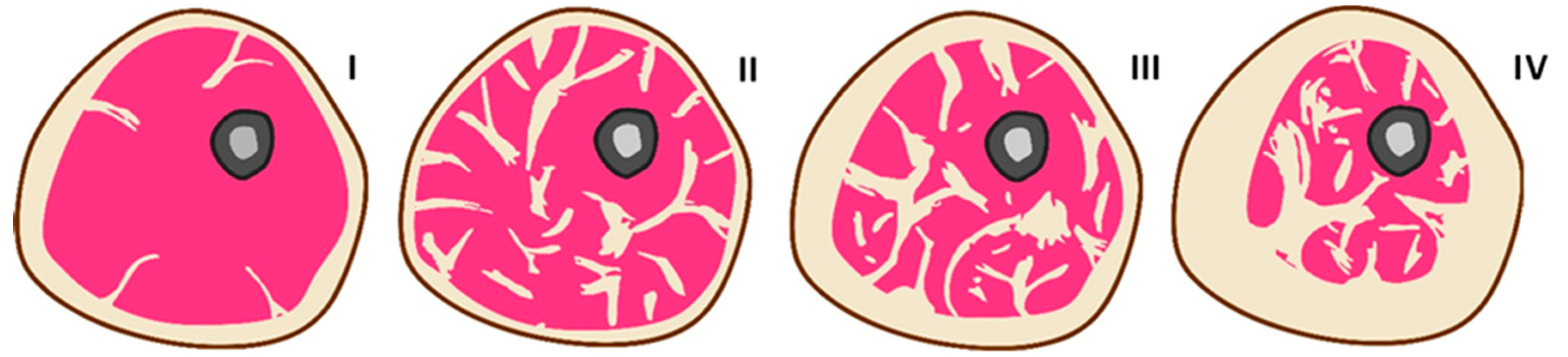
Figure 2.
Ultrasonic tissue phantom: 1 – acoustic window; 2 – acoustically transparent membranes; 3 – 3D-printed mold; 4 – “muscle tissue” section; 5 – periodic oil-filled holes mimicking IMAT; 6 – oil-filled sections mimicking SAT.
Figure 2.
Ultrasonic tissue phantom: 1 – acoustic window; 2 – acoustically transparent membranes; 3 – 3D-printed mold; 4 – “muscle tissue” section; 5 – periodic oil-filled holes mimicking IMAT; 6 – oil-filled sections mimicking SAT.
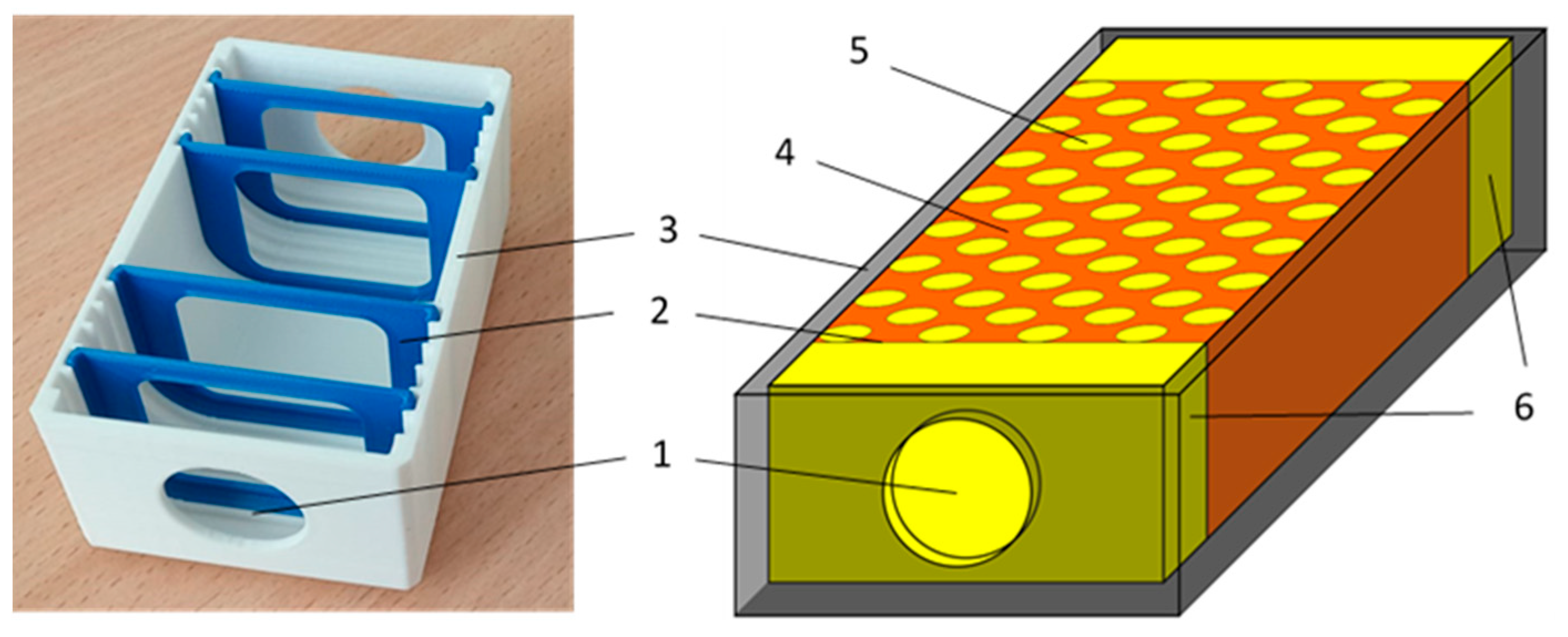
Figure 3.
3D printed dies with regular holes for creating IMAT gradations.
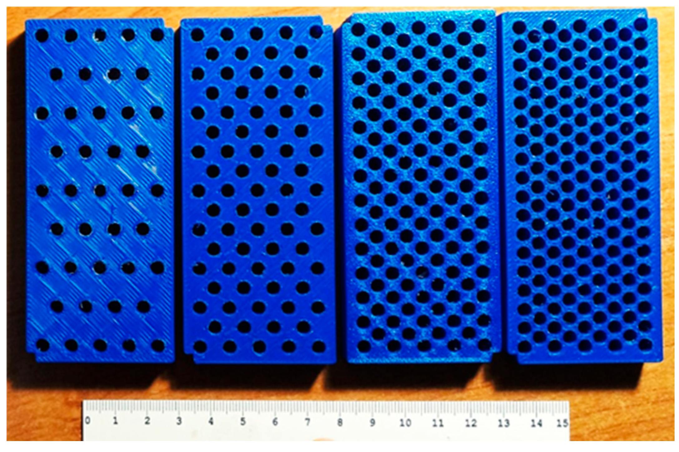
Figure 4.
Experimental setup: 1 – muscle tissue phantom; 2 – ultrasound receiving transducer; 3 – ultrasound emitting transducer; 4 – digital caliper; 5 – reinforced consoles; 6 – ultrasonic acquisition unit; 7- laptop PC.
Figure 4.
Experimental setup: 1 – muscle tissue phantom; 2 – ultrasound receiving transducer; 3 – ultrasound emitting transducer; 4 – digital caliper; 5 – reinforced consoles; 6 – ultrasonic acquisition unit; 7- laptop PC.
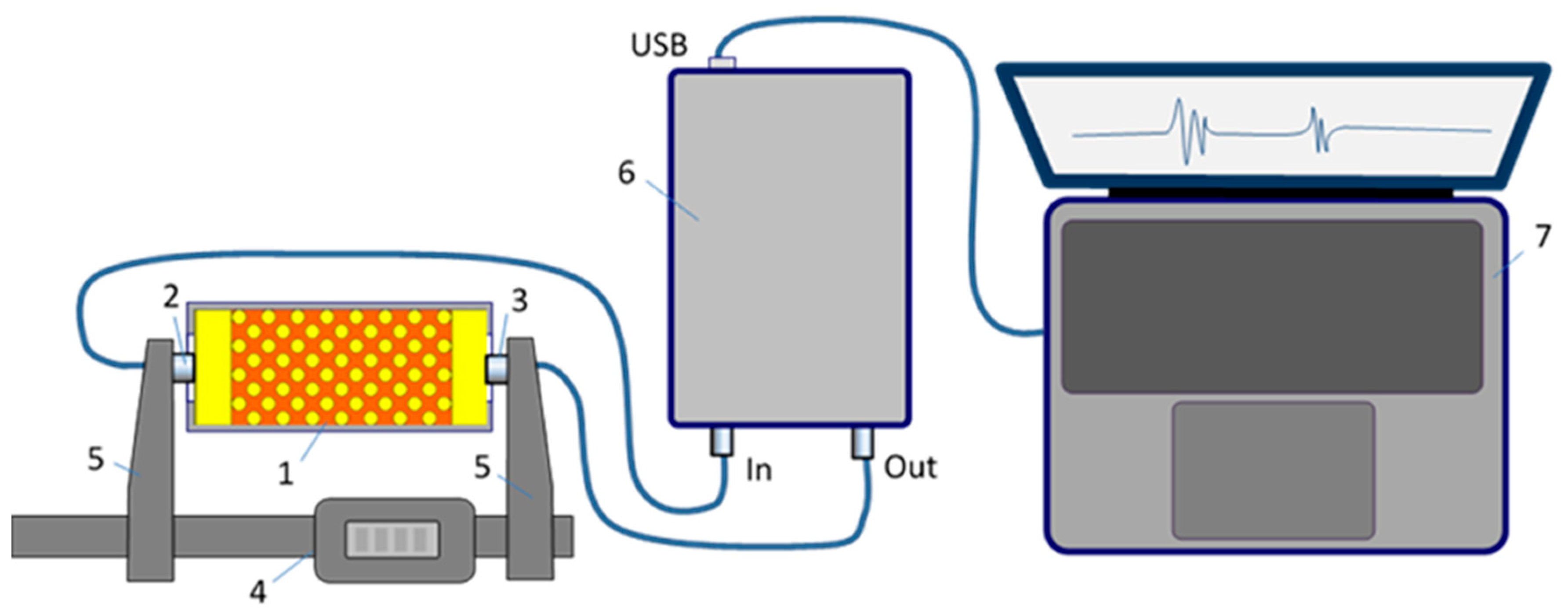
Figure 5.
Train of ultrasonic signals acquired in one run (upper chart), expanded signal fragments in time scale within dashed areas (left column charts) and their spectra in frequency domain (right column charts). D1 and D2 – direct propagation signals at 2.5 and 0.8 MHz excitation Ex1 and Ex2; D3 – direct propagation signal excited by frequency sweep Ex3; R3 – reflected frequency sweep signal.
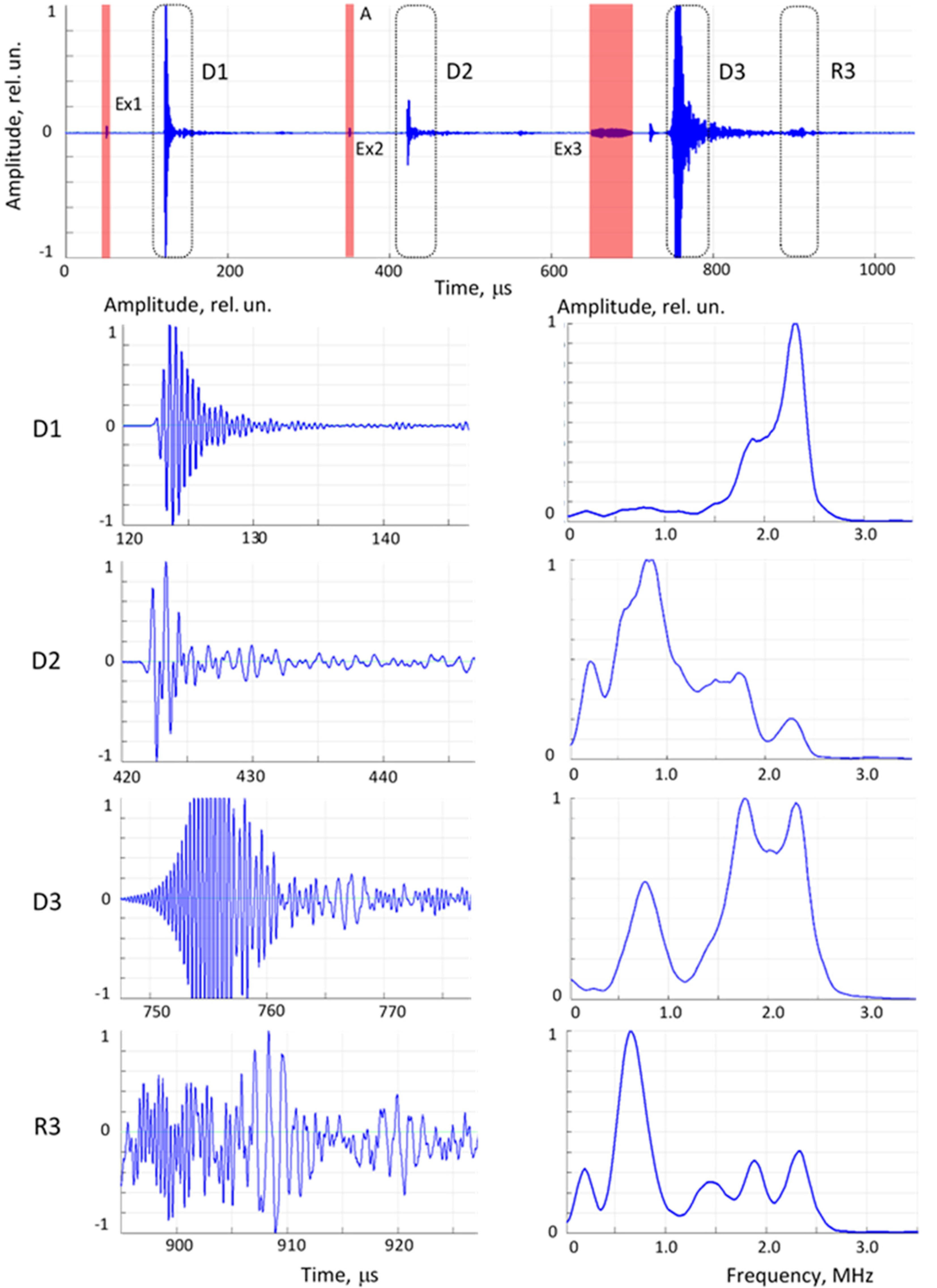
Figure 6.
Objects (phantoms) grid according to simulated gradations of SAT and IMAT.
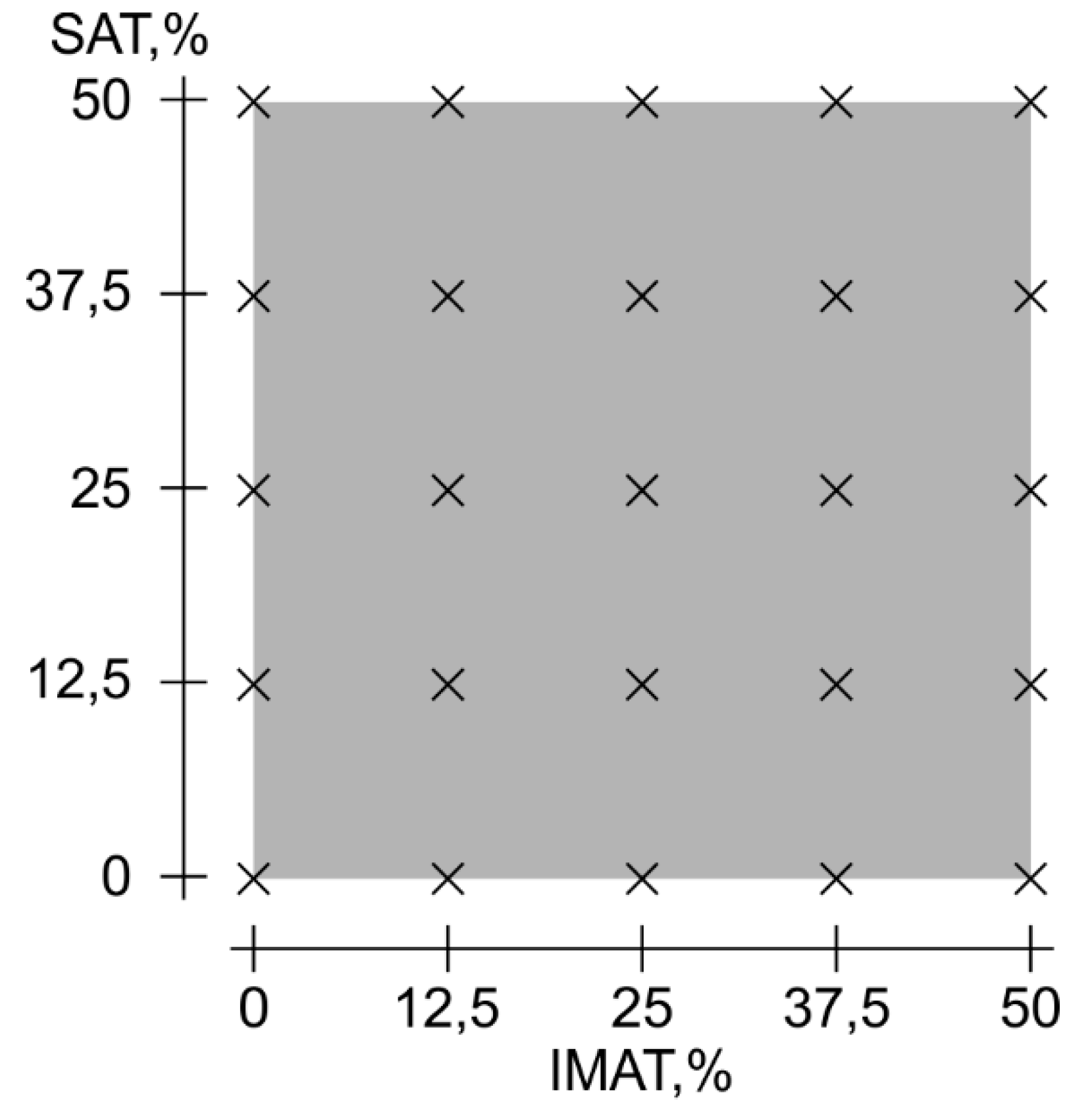
Figure 7.
Recognition procedure using decision rules: A – determination of intersection of on criterion Cr of a test object with three-dimensional minimum-maximum volume of Cr determined by training set; B – two-dimensional area of possible answers by criterion Cr; C – final answer as intersection area of all criteria.
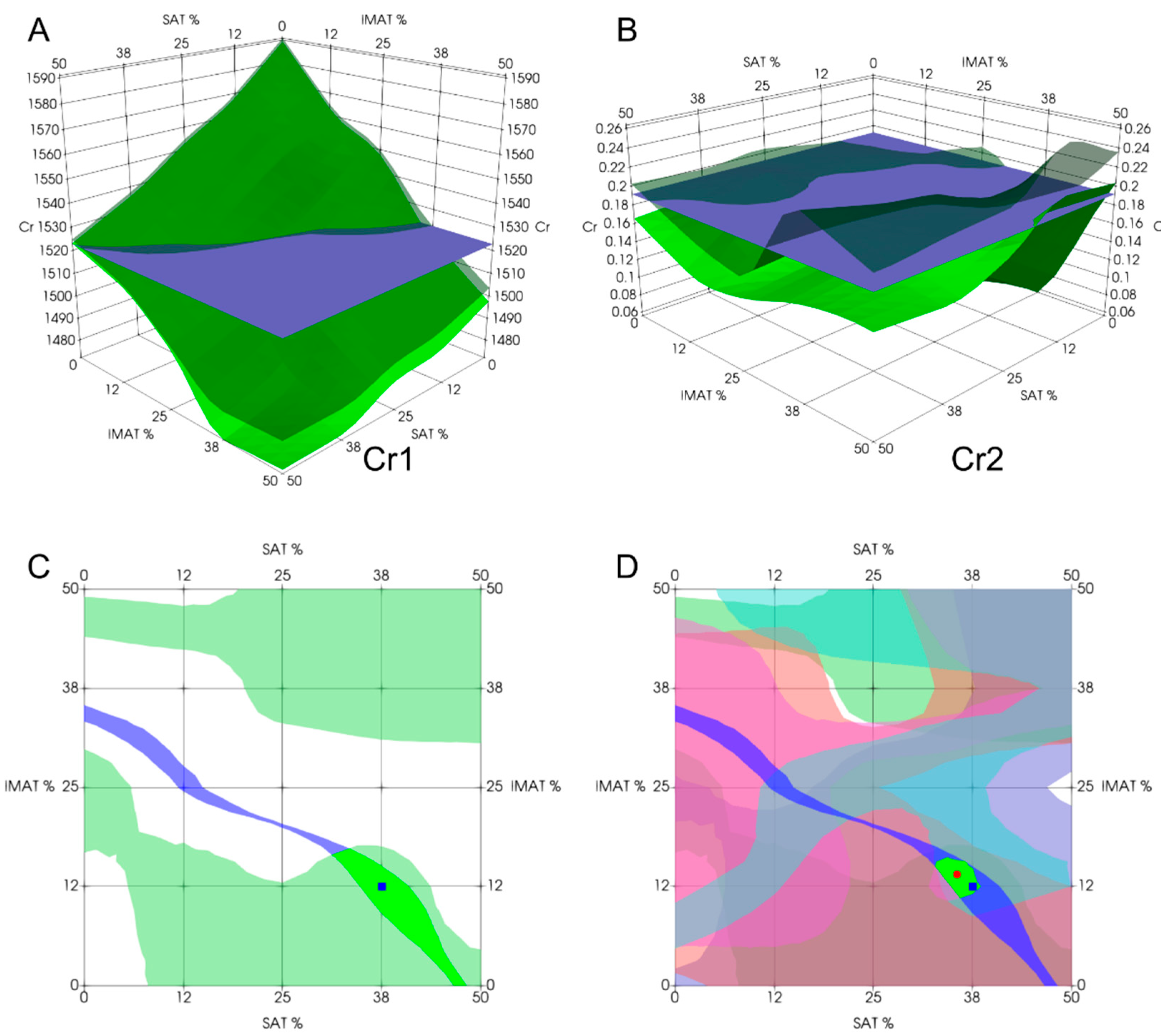
Figure 8.
Structure of LSTM cell.
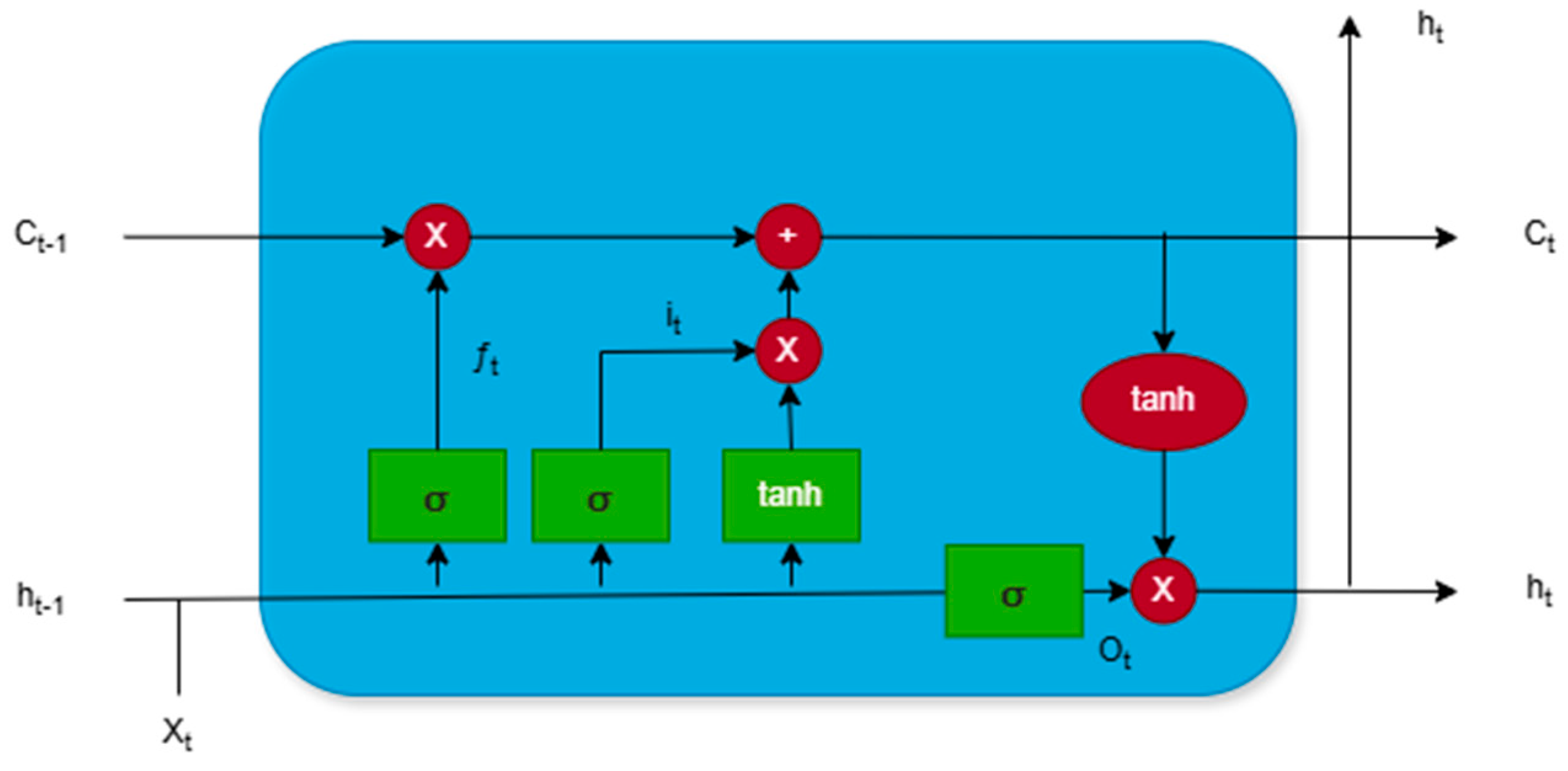
Figure 9.
Experimental decision rules constructed for evaluation criteria Cr1- Cr6 (A-F) in 3-dimensional domain as piecewise linear functions of SAT and IMAT.
Figure 9.
Experimental decision rules constructed for evaluation criteria Cr1- Cr6 (A-F) in 3-dimensional domain as piecewise linear functions of SAT and IMAT.
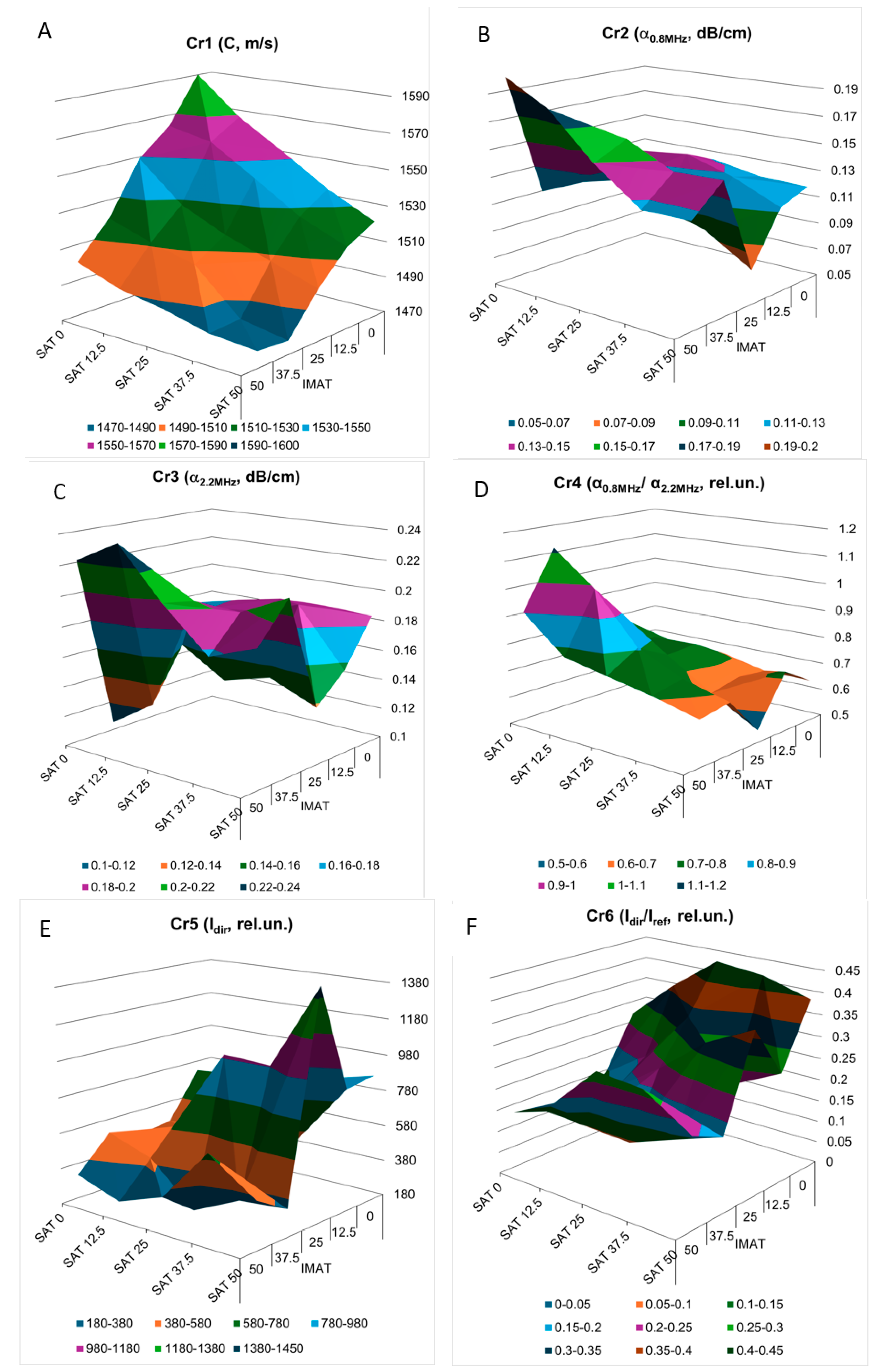
Figure 11.
Examples of differential estimation of SAT and IMAT using decision rules. (Green area – intersection of the maximum number of decision rules; green square – predicted value; and red circle – experimental estimation). The top and bottom rows of graphs illustrate examples of precise and dispersed evaluation estimation, respectively.
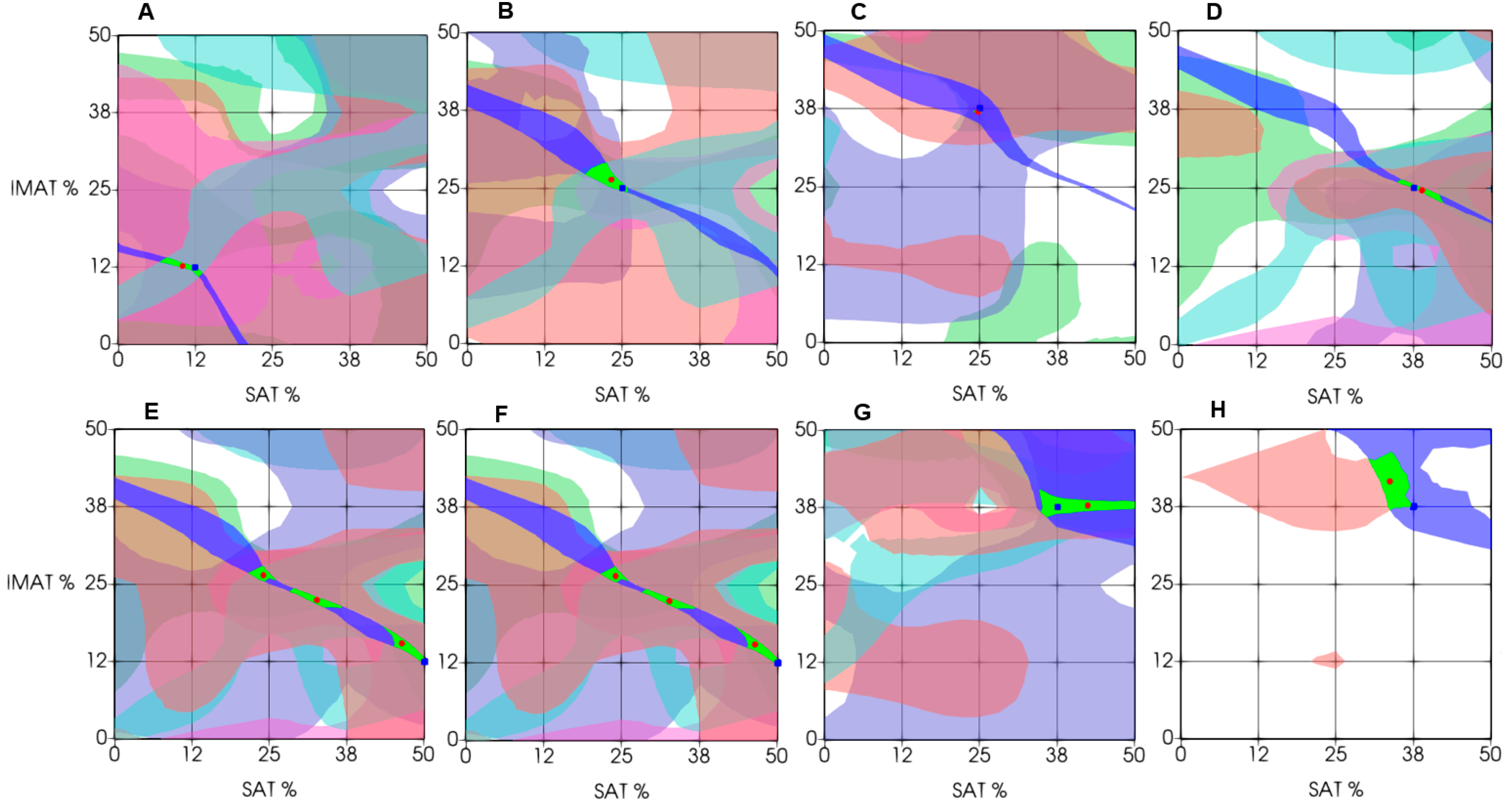
Figure 12.
Structure of LSTM network.
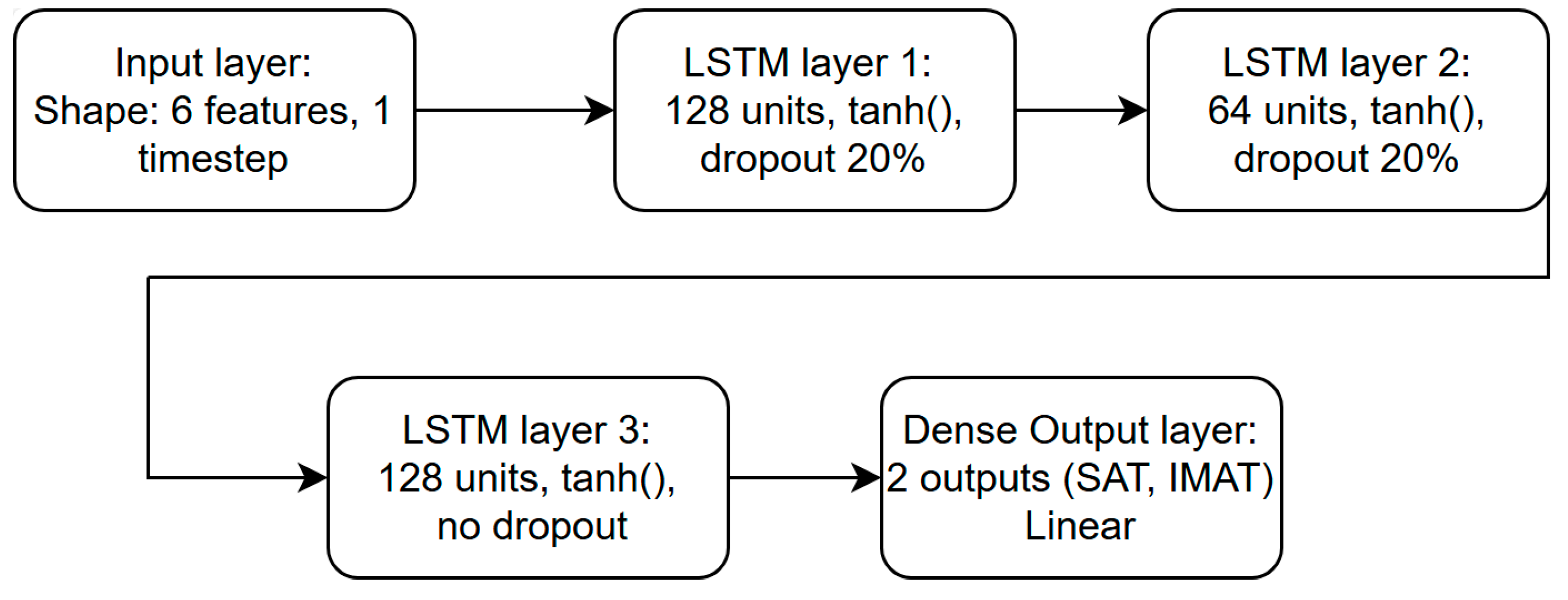
Figure 13.
Topology of evaluation errors of SAT and IMAT by SAT-IMAT distribution field using PR/DR and ANN/ LSTM.
Figure 13.
Topology of evaluation errors of SAT and IMAT by SAT-IMAT distribution field using PR/DR and ANN/ LSTM.
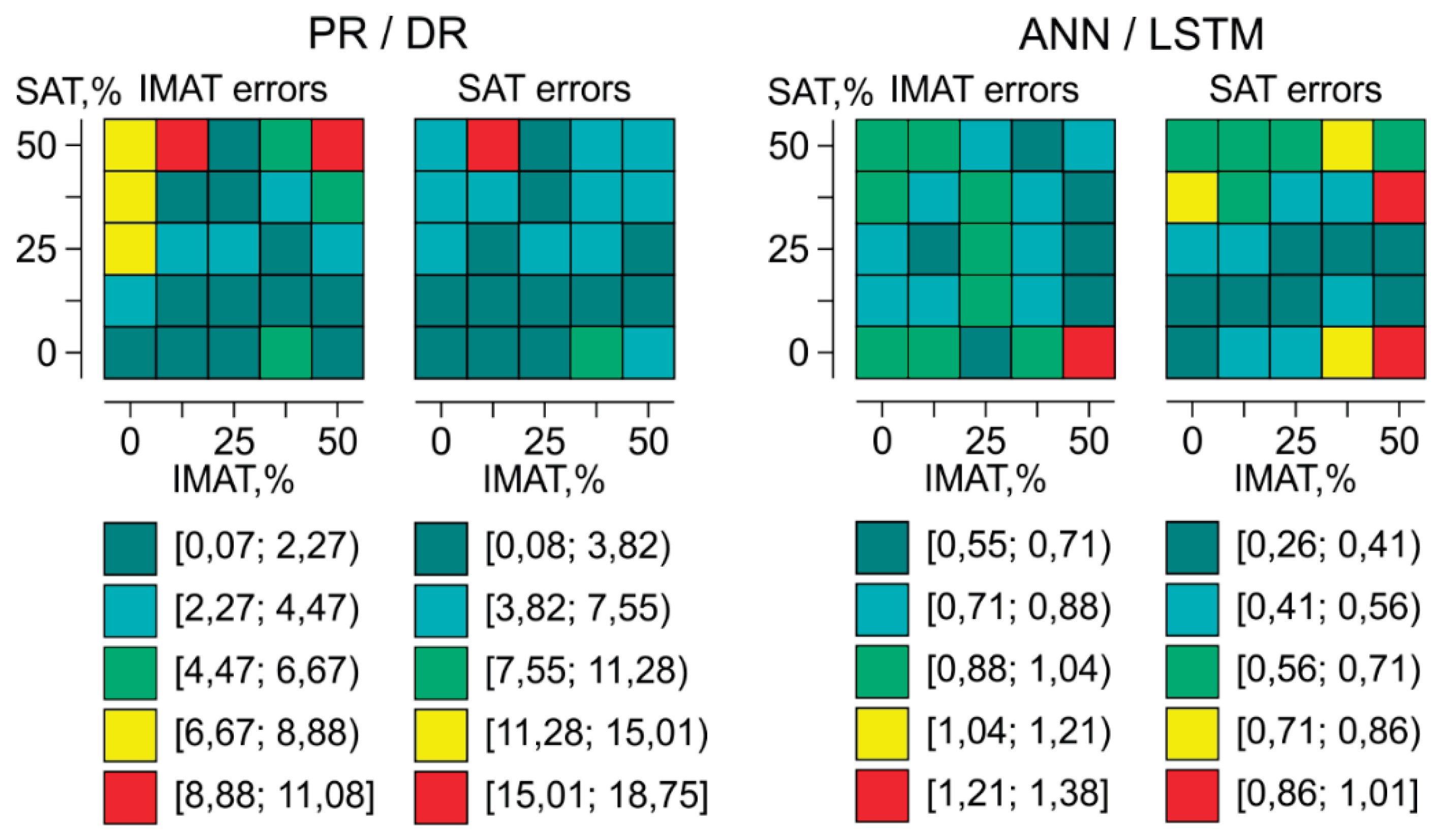

Table 1.
Statistical measures of evaluation criteria.
| Criterion | Cr1 | Cr2 | Cr3 | Cr4 | Cr5 | Cr6 |
| Measurement unit | m/s | dB/cm | dB/cm | rel.un. | rel.un. | rel.un. |
| Mean for the entire data set (M) | 1520.0 | 0.131 | 0.745 | 0.177 | 0.235 | 594.8 |
| Standard deviation for the entire data set (SD.m) | ±30.3 | ±0.028 | ±0.139 | ±0.033 | ±0.113 | ±307.1 |
| Coefficient of variation for the entire data set (CV.m) | 2.0% | 21.4% | 18.7% | 18.4% | 48.2% | 51.6% |
| Mean standard deviation for the individual objects (SD.o) | ±1.31 | ±0.012 | ±0.059 | ±0.013 | ±0.034 | ±102.8 |
| Mean coefficient of variation for individual objects (CV.o) | 0.1% | 9.4% | 7.9% | 7.2% | 14.6% | 17.3% |
| Index of individuality (II = CV.o/ CV.m) | 0.04 | 0.44 | 0.42 | 0.39 | 0.30 | 0.33 |
| Reciprocal of II (RII = 1/II) | 23.2 | 2.3 | 2.4 | 2.6 | 3.3 | 3.0 |
Table 2.
Comparison of mean evaluation errors (percentage) for SAT and IMAT using pattern recognition PR/DR and artificial neural networks ANN/LSTM.
Table 2.
Comparison of mean evaluation errors (percentage) for SAT and IMAT using pattern recognition PR/DR and artificial neural networks ANN/LSTM.
| Data splitting | PR/DR | ANN/LSTM | ||
| IMAT | SAT | IMAT | SAT | |
| Split 1 | 3.88 ± 3.61 | 5.25 ± 5.20 | 0.74 ± 0.32 | 0.37 ± 0.26 |
| Split 2 | 3.06 ± 3.80 | 4.52 ± 4.58 | 0.40 ± 0.30 | 0.34 ± 0.23 |
| Split 3 | 2.97 ± 3.15 | 4.29 ± 3.79 | 1.20 ± 0.62 | 0.45 ± 0.43 |
| Split 4 | 3.36 ± 3.76 | 3.84 ± 3.80 | 0.48 ± 0.33 | 0.65 ± 0.34 |
| Split 5 | 3.75 ± 4.94 | 5.08 ± 7.34 | 0.46 ± 0.28 | 0.41 ± 0.27 |
| Average error across all splits | 3.14 ± 3.85 | 4.60 ± 5.06 | 0.65 ± 0.49 | 0.41 ± 0.27 |
Disclaimer/Publisher’s Note: The statements, opinions and data contained in all publications are solely those of the individual author(s) and contributor(s) and not of MDPI and/or the editor(s). MDPI and/or the editor(s) disclaim responsibility for any injury to people or property resulting from any ideas, methods, instructions or products referred to in the content. |
© 2025 by the authors. Licensee MDPI, Basel, Switzerland. This article is an open access article distributed under the terms and conditions of the Creative Commons Attribution (CC BY) license (http://creativecommons.org/licenses/by/4.0/).
Copyright: This open access article is published under a Creative Commons CC BY 4.0 license, which permit the free download, distribution, and reuse, provided that the author and preprint are cited in any reuse.


