
Submitted:
03 November 2025
Posted:
03 November 2025
You are already at the latest version
Abstract
We present a unified framework for modeling the term structure of interest rates using both the affine term structure models (ATSM) with jumps and regime-switches. The novelty lies in combining affine jump diffusion models with regime-switching dynamics within a unified framework, allowing for state-dependent jump behavior while preserving analytical tractability. This integration enables the model to simultaneously capture nonlinear market regimes and discontinuous movements in interest rates—features that traditional affine models or regime-switching models alone cannot jointly represent. Estimation is carried out using the unscented Kalman filter (UKF) with the believe that it is capable of handling nonlinearity, therefore should estimate the non-Gaussian dynamics well. The yield curve fitting demonstrate that both models fit our data well. RMSEs show that the regime-switching affine jump diffusion (RS-AJD) models outperforms the affine jump diffusion (AJD) in-sample.
Keywords:
regular affine process
; Levy jump process
; regime switching
; stylised facts
; non-Gaussian residuals
1. Introduction
Bond yields and their returns are not normally distributed, thus overruling the concept of symmetry around the mean. They retain non-normal features, such as fat tails, skewness, and volatility clustering (Piazzesi 2010).
ATSMs augmenting with jumps or regime-switching dynamics offer enhanced flexibility to capture these stylised facts observed in interest rate data (Piazzesi 2010; Singleton 2006). When used to fit the term structure of interest rates, these models often lead to a reduction in the Root Mean Squared Error (RMSE) and produce residuals that more closely approximate Gaussian white noise. This improvement reflects better model specification and a more accurate representation of interest rate dynamics. Standard Gaussian ATSMs often fall short in capturing abrupt market movements or structural shifts. Incorporating jumps or regime-switching mechanisms allows the model to internalise these dynamics, thereby improving both in-sample fit and the statistical properties of residuals (Dai and Singleton 2000; Duffie and Kan 1996a).
Jumps are popularly associated with scheduled macroeconomic news release, typically the Central Banks announcing the interest rates changes. ATSMs class is not completely affine except for special cases as found in Hamilton (1989),Dai and Singleton (2000) and Ang and Bekaert (2002). This class of regime switching models exhibit commonly two regimes, high-persistence low-volatility, and a low-persistence high-volatility (Piazzesi 2010).
Extension of affine diffusion models to AJD is accomplished by including a Levy type jump to them. Duffie et al. (2000) discusses the AJD in terms of no-arbitrage, analytical tractibility and their impact regarding accuracy with which they price bonds and their derivatives. Cont et al. (2004) discusses various Levy processes, their nature, whether finite or infinite jumps and their impact on the difussion. The associated stylised facts for these AJD is also exhibited by volatilty skews and the behavior of options. Another important aspect to the term structure modelling and pricing of jump models is the market price of risk, in particular, consideration for compensartion from the jump risk. Regime switching models are expected to be free from arbitrage, analytically tractable and offer closed-form solutions.
A growing body of literature considers the treatment of regime detection through implementation of the Markov-modulated models; see Hu (2022), Qin et al. (2024), and Ding et al. (2025) among others. Regarding jumps within regime switching models, we consider the approach involving a marked point process by Landen (2000). This procedure determines the intensity kernel and regime-based risk compensation. Our study seeks to link the jumps to regimes even though they arise from different circumstances. Our focus has more to do with the ability of jumps and regime switching models to fit the term structure of interest rates when non-Gaussian dynamics are present. Effectiveness of these models should be confirmed by a reduction of the root-mean-square errors (RMSE), and improvement from non-Gaussian residuals shifting more towards Gaussian.
In this study we consider a continuous-time modelling in regimes, contrary to previous work involving mostly discrete-time, Dai et al. (2007), Ang and Timmermann (2012) among others. We also consider a non-Gaussian approach, unlike the Gaussian asumption made by Dai et al. (2007). Bandara and Munclinger (2011) also follow the continuous-time approach but their estimation strategy differ from ours as they use the Kalman filter. We estimate the model using the UKF for its known capability to handle nonlinearity.
We follow the AJD from the empirical work by Duffie et al. (2000), and the canonical form of parameters by Dai and Singleton (2000), from which we adopt the closed-form and tractability in pricing of bonds and derivatives. The bond yields derived from these models are tested for fitting our data when jumps are introduced. The same process is extended to regime switching models from which we expect regime switching analogue to the AJD, with certain parameters restrictions. We consider an affine process X whose characteristic function takes the form
where state vector at time t, u is a complex or real vector argument in the characteristic function, and are complex valued functions, and ⊤ a transpose operation for a matrix . The parameters within are expected to vary with regimes while those within do not.
Our argument regarding the affine jump diffusion and subsequently the regime switching affine models is triggered by the definition and characterisation of the regular affine process from Duffie et al. (2002). A generator-based approach is then followed on how a Markov process X evolves over time (Duffie et al. 2002; Keller-Ressel et al. 2011). In the context of regime switching models, the generator should also define the dynamics that characterise both the continuous-time and discrete-time stochastic dynamics. The final output is the regime-specific characteristic function and a set of regime-specifc ordinary differential equations (ODE) or Ricatti-type equations from which a Duffie and Kan (1996a) style zero-coupon bond price P maturing at time , hence the yield is derived. Extension of the regular affine process to the regime switching formulation is the condition for a regme switching affine models (Van Beek et al. 2020). In addition, we follow Landen (2000) by incorporating the kernel intensity for regimes to ensure that analogous with the jump kernel intensity, the model enables the pricing of regime risk.
Our key contributions are threefold. First, we formally demonstrate that the regular affine process specification naturally extends RS-AJD models. Second, we employ the UKF for efficient state estimation and model calibration, which enables accurate yield curve fitting in the presence of latent factors and nonlinearities. Third, empirical results show that the fitted models produce residuals that closely approximate Gaussian white noise, as confirmed through residual diagnostics and Q-Q plots—indicating improved model specification and robustness in capturing interest rate dynamics.
The remainder of the paper is structured as follows: Section 2 discusses briefly a literature review; Section 3 describe the model framework and estimation strategy; Section 4 discusses data collection; Section 5 discusses the scenarios; Section 6 discusses the model implementation; Section 7 discuses the analysis of results. Section 8 concludes.
2. Literature Review
The modeling of term structure of interest rates has undergone significant development over the past three decades, with ATSMs emerging as a dominant framework due to their analytical tractability and empirical flexibility. Early models such as Vasicek (1977) and Cox et al. (1981) provided foundational single-factor Gaussian and square-root processes, but these were insufficient to capture the richness of the yield curve observed in empirical data. The extension to multi-factor affine models was formalised by Duffie and Kan (1996b), who derived the zero-coupon bond equation as an exponetially affine function of the state variable X.
Dai and Singleton (2000) introduced the specification analysis for ATSMs which determines whether they are well-defined for bond pricing, "admissibility". They defined the family of affine models, where N is the number of factors and denotes the number of volatility components. Within this structure, the models represent the purely Gaussian and homoskedastic affine class, where none of the state variable X affect its volatility at time t. models with is characterised by the assumption that one of the X’s determines the conditional volatility of all three state variables. This specification introduces the short rate dynamics such as mean-reversion, central tendency and stochastic volatility leading to a shift in the normal distribution.
Affine term structure models permit deviations from normality primarily through the incorporation of stochastic volatility and the introduction of jump components. Distinguishing between these sources of non-normality using only first and second moments — such as mean and variance — is inherently challenging, as both features can produce similar effects on volatility clustering and heavy-tailed behavior in returns. Regime switching models also produce non-normal return distributions and consistent with empirical evidence of nonlinearities in the conditional first moments of financial time series. By allowing parameters such as drift or volatility to shift across latent regimes, these models can capture structural breaks, asymmetries, and time-varying risk premia that are otherwise difficult to model within standard linear frameworks; see Piazzesi (2010) and references therein.
Singleton (2006) investigated the recurrent non-normal features observed in yield return distributions, particularly during periods of peak or quite financial market volatility. These deviations from Gaussianity are often attributed to time-varying volatility and sudden, infrequent price movements. The latter is typically modeled via classical jump processes, such as Poisson jumps, or more generally through Lev́y-type processes. Other approaches include drawing shocks from mixtures of distributions or introducing regime-switching structures that allow for discrete shifts in model parameters. Jump processes capture abrupt discontinuities, whereas regime-switching models emphasise shifts between persistent economic states. Singleton (2006) further explored how these mechanisms interact with stochastic volatility — initially in discrete-time settings and subsequently within continuous-time affine frameworks that incorporate both stochastic volatility and jump components. Together, these enhancements aimed to replicate the observed skewness, kurtosis, and tail behavior in bond yield and return distributions, especially across different market conditions.
Duffie et al. (2000) presented an AJD that provide an analytical treatment of a class of transforms, including various Laplace and Fourier transforms as special cases, that allow a solution for a range of valuation and econometric problems. This AJD is a process for which the drift vector, instantaneous covariance matrix, and jump intensities all have affine dependence on the state vector X. They extended the existing literature on affine asset pricing models by deriving a closed-form expression for an extended transform of an AJD process X, and showed that this transform leads to analytically tractable pricing relations for a wide variety of valuation problems. Piazzesi (2000) applies the extended transform differently in the treatment of term-structure models with releases of macro-economic information and with central-bank interest rate targeting.
Regime switching affine models should inherit similar characteristics to AJD of tractability and close-form solutions. The work of Van Beek et al. (2020) addressed this issue by evaluating the prevalance of regular affine process and parameter restrictions within the regime switching. They prove that the joint process of the Markov chain and the conditionally affine part is a process with an affine structure on an enlarged state space, conditionally on the starting state of the Markov chain. The process leads to regime-specific characteristic functions and the solution of ODE as it is the case with regular affine process. Essentially, a pricing solution based on an affine process is extended to a regime switching affine process without sacrificing the analytical tractability of the affine process. They consider among several empirical option pricing applications, a diffusion type short rate model of Landen (2000), which falls within the category of hidden Markov models. In this model the underlying Markov process is assumed to have a stochastic differential driven by Wiener processes and a marked point process. They also consider the bond valuation application of Elliot and Siu (2013) on short rate models, who establish a Markov-modulated exponential-affine bond price formula with coefficients given in terms of fundamental matrix solutions of linear matrix differential equations.
Zhu et al. (2015) developed Feynman-Kac formulas for a class of regime-switching jump diffusion processes. In these models the jump part is driven by a Poisson random measure associated to a general Lev́y process and the switching part depends on the jump diffusion processes.
In this paper we adapt the regular affine process by Duffie et al. (2002) and their formulations together with those from Keller-Ressel et al. (2011). The AJD part is extended to the regime part accordingly to evaluate the regime-specific formulation of the characteristic function, the generators, and the bond pricing equation. Our objective is to model first, the AJD, followed by the regime switching models in the realm of the regular affine process. In contrast with Dai et al. (2007) who assume a Gaussian distribution and discrete-time process, we assume that the yields and their returns are non-normal.
A growing body of literature highlights the limitations of standard Kalman filtering in the context of nonlinear and non-Gaussian dynamics, particularly in fixed income modeling. Christoffersen et al. (2013) show that the UKF significantly outperforms the Extended Kalman Filter (EKF) in affine term structure models due to its ability to better handle nonlinearities without requiring Jacobian computations; see also Hirsa (2024). Their findings support the UKF as a viable estimation tool for fixed income applications.
Chourdakis (2002) motivates the need for estimation methods that can accommodate both jumps and regime switching in continuous-time models, noting that traditional Gaussian-based filters may fail to capture the irregularities introduced by such dynamics. Although developed outside of finance, the Generalized Maximum-likelihood UKF (GM-UKF) introduced in robust control literature Liu et al. (2017) offers further motivation by demonstrating how robust filtering approaches can mitigate the impact of non-Gaussian noise—precisely the type of issue that arises in affine jump diffusion models with regime switching. Building on these insights, we adopt a UKF-based estimation strategy tailored to capture the nonlinear, regime-dependent, and non-Gaussian features of the term structure under jump-risk and switching dynamics.
3. Model Establishment
Affine processes are a class of Markov chain characterised by the property that their logarithmic characteristic functions are affine in the initial state. They are typically defined through their infinitesimal generators, which involve parameters such as drift, diffusion, and jump intensity functions, each depending affinely on the current state. Under suitable regularity conditions, the evolution of the characteristic function is governed by a system of Riccati-type (ODEs) parameterised by time and initial conditions (Duffie et al. 2002; Keller-Ressel et al. 2011).
A natural extension of this framework is the regime-switching affine process, in which the model parameters — and hence the generator — are modulated by an underlying finite-state Markov chain. This regime-specific structure enables the model to capture structural changes in the dynamics, such as shifts in volatility, mean reversion, or jump activity, driven by the regime variable. The process is expected to exhibit the affine behavior, conditioned on the current regime, while preserving analytical tractability through a system of ODEs that characterise the evolution of the characteristic function under each regime (Van Beek et al. 2020).
The Markov-modulated component builds upon the marked point process framework of Landen (2000), adapted here to ATSMs with jumps and regime dependence.
Proposition 1
(Affine Process). Let be a time-homogeneous Markov process with state space , adapted to a filtered probability space , and satisfying the Feller property ( a central regularity condition in the theory of affine processes, particularly when ensuring existence, uniqueness and well-behaved semigroups). The process is said to be affine if there exist deterministic functions
such that the conditional characteristic function of , given , admits the exponential-affine form:
Proposition 2
(Affine Jump-Diffusion). Let be a time-homogeneous Markov process satisfying the following SDE:
where:
- is a constant drift vector and a loading matrix;
- is the volatility matrix;
- is a non-negative affine process driving stochastic volatility;
- is a standard Brownian motion;
- is the jump Poisson random measure associated with ;
- is the compensated jump measure;
- is the Lévy measure, governing the distribution of jump sizes .
The diffusion term introduces stochastic volatility while preserving the affine structure. This framework allows the derivation of bond price equations via generalised Riccati equations. As shown in Duffie and Kan (1996a), models in the affine class admit bond price expressions that are exponentially affine in the state variables under an affine short rate specification.
3.1. Regime Switching Affine Processes
The classical AJD framework, as developed by Duffie et al. (2000), provides a powerful and tractable class of models where characteristic functions admit closed-form or semi-closed-form solutions. Empirical evidence suggests that financial markets exhibit distinct regimes characterised by shifts in volatility, jump intensity, and mean-reversion levels (Ang and Bekaert 2002; Ang and Timmermann 2012; Hamilton 1989) among others. These regime shifts cannot be captured adequately by a single affine jump-diffusion process.
The AJD is extended to RS-AJD as a continuous-time Markov chain on a specific state space that switches between the states. Importantly, this extension preserves the affine structure, thereby retaining analytical tractability while allowing for richer dynamics that reflect regime changes (Van Beek et al. 2020).
We now extend Proposition 2 to its regime switching counterpart as follows:
Proposition 3
(Regime-Switching Affine Jump Diffusion (RS-AJD)). Let be a continuous-time, finite-state Markov chain with generator matrix , where .
Let satisfy the stochastic differential equation: Let satisfy the stochastic differential equation:
where:
- is a drift vector in regime , and a loading matrix in regime ;
- is the regime-dependent volatility matrix;
- is a non-negative stochastic process governing volatility;
- is a standard Brownian motion;
- is the compensated jump measure under regime ;
- is the regime-specific Lévy measure governing jump intensity and size distribution;
- denotes the support of jump sizes ξ.
The regime process is a pure jump Markov chain with jump measure on , and compensator:
where denotes the Dirac measure at point .
The compensated jump measure of Z is defined by:
The stochastic integral representation of is:
and the semimartingale decomposition of is:
Thus, the full process is a Markov semi-martingale with regime-dependent drift, diffusion, and jump components.
Proof:
See Appendix A.
3.2. Generator of the Regime Switching Affine Process
The infinitesimal generator provides a compact way to describe the local behaviour of a Markov process (Duffie et al. 2000). In our model, the joint process is a RS-AJD, with
Fix , and let be a twice continuously differentiable function. The conditional infinitesimal generator of the state process under fixed regime z acts on f as:
where:
- is the gradient of f.
- is the Hessian of f.
The volatility scaling matrix describing state-dependent volatility scaling under regime z is specified as
where:
- is the constant term (intercept) for the i-th component of the volatility scaling in regime z.
- is the loading (sensitivity) of the i-th volatility component to the j-th state variable , under regime z.
- indexes the volatility components, i.e., the diagonal entries of .
- indexes the state variables.
This generator captures the combined effects of drift, diffusion, and jumps under a given regime. The jump intensity and the Lévy measure may vary with the regime, allowing for flexible modeling of rare or discontinuous events.
Joint Generator for
To describe the full process , we combine the regime-specific generator with the generator matrix of the finite-state Markov chain , where for and . Then for any function , the joint infinitesimal generator is given by:
The first term describes the evolution of under a fixed regime z, while the second term accounts for regime-switching jumps governed by the generator matrix Q.1
The affine structure of the RS-AJD model ensures that expectations of exponential-affine functions — such as characteristic functions or bond prices — can be computed from a system of ODEs. Specifically, for a short rate of the form
with regime-dependent parameters , , pricing a zero-coupon bond reduces to solving a system of regime-specific Riccati equations derived from the generator .
This generator-based formulation plays a central role in deriving semi-analytical solutions for prices, expectations, and moment-generating functions in a regime-specific and computationally tractable manner.
Under the risk-neutral measure , define the zero-coupon bond price as
Let
Then f satisfies the partial integro-differential equation (PIDE)
We postulate the affine
with deterministic functions , , and terminal conditions
Subsrituting the affine (11) into the PIDE, applying the generator , and matching coefficients in powers of x yields a system of coupled ODEs (Riccati equations) for :
Here is the affine function of corresponding to regime z, and the sum over reflects regime transitions through the Markov generator Q. are the terminal conditions.
3.2.1. Bond Yields and Term Structure
From the solution of and , the zero-coupon bond price in regime z takes the exponential-affine form (Landen 2000; Wu and Zeng 2004)
when the current regime is z. More generally, if a regime is not observed or transitions are probabilistic, priced value becomes a regime-weighted mixture:
where or an equivalent regime probability.
The continuously compounded yield is
which retains an affine form in the state vector and depends on regime probabilities.
Given that the process is a semi-martingale, it admits a well-defined stochastic integral formulation, allowing us to work within a no-arbitrage pricing framework. For tractability, we assume that the market price of risk is zero, implying that the physical measure coincides with the risk-neutral measure . Under this assumption, the model dynamics can be interpreted directly under , and no change-of-measure adjustment is necessary for pricing.
3.3. Joint Dynamics of State and Regime Processes
Following the specification of Landen (2000) and Wu and Zeng (2004), we consider a joint affine jump-diffusion system for the latent state process and the discrete-valued regime process . These processes evolve in continuous time and interact dynamically through their drift, volatility, and jump intensities.
State Process :
The dynamics characterised in Proposition 3 can alternatively be expressed in the form of a SDE for the state process , which evolves under a regime-dependent affine jump-diffusion specification:
where:
- is a compensated marked point process driving jumps in ,
- denotes the jump size in the state space.
Regime Process :
The evolution of the regime is modeled via a marked point process:
where:
- is the mark space of regime transitions,
- for , mapping the transition to the new regime index,
- is a compensated marked point process governing regime jumps.
State-Dependent Regime Transition Intensity:
The stochastic intensity of regime switching is allowed to depend on the current state . The compensator (or intensity measure) of the regime-jump process is given by:
where:
- denotes a transition from regime i to j,
- is a measurable state-dependent transition intensity,
- is a reference measure over the mark space .
We follow Wu and Zeng (2004) in assuming that the transition intensity is exponentially affine in the state
where and are parameters specific to the transition . This choice ensures both tractability and consistency with the affine term structure framework.
(17) describes a multi-factor affine jump-diffusion process for the latent state variables , whose parameters depend on the prevailing regime . Simultaneously, (18) captures endogenous regime transitions via a marked jump process, where the intensity of switching from regime i to j is driven by the current economic state through an exponential-affine function (20).
This joint specification allows regime switching to be triggered endogenously by macro-financial conditions, thereby embedding jump risks and regime-dependent dynamics within a unified affine framework.
3.4. Estimation Framework
We consider modeling the term structure of interest rates using a nonlinear state-space framework, where observed yields are driven by latent factors . This section outlines the estimation strategy based on the UKF for two affine models, the AJD and the RS-AJD.
3.4.1. State-Space Modeling and UKF Estimation of Affine Yield Curve Models
Recent advances in the literature, (Cheng et al. 2024; Christoffersen et al. 2013; Deng 2023; Lv et al. 2025) emphasise the need for flexible estimation frameworks that can accommodate nonlinearities and deviations from Gaussian assumptions. Christoffersen et al. (2013) show that the UKF offers significant improvements over the EKF when applied to affine term structure models, due to its ability to more accurately approximate nonlinear transformations without requiring Jacobians. Their findings support the UKF as a practical and robust estimation strategy in fixed income applications.
In light of this, and the fact that our models incorporate both jumps and regime-switching dynamics, we adopt the UKF to estimate latent states and parameters. The UKF is particularly suitable here, as it efficiently handles the nonlinear, non-Gaussian features that arise from jump components and regime-dependent behavior.2
3.4.2. State (Transition) Equation
The state variables transition equations take the Euler-Maruyama approximation form of respective SDEs. The latent factor process follows a discrete-time approximation of a jump-diffusion process:
where:
- is the drift function,
- is the diffusion (volatility) function,
- is standard Gaussian noise,
- is the jump component, where and the jump sizes are i.i.d. and independent of and .
In the UKF implementation, the jump component is approximated as Gaussian with:
which is incorporated into the process noise covariance.
The transition function used in the UKF is:
with total process noise covariance:
3.4.3. Measurement Equation
The observed yield vector is modelled as an affine function of the latent state:
where:
- is a vector of intercept terms,
- is the factor loading matrix,
- is measurement noise.
The measurement function for the UKF is:
3.4.4. UKF in Regime-Switching Jump-Diffusion (RS-AJD) Model
To capture the structural changes in yield dynamics, we extend the model to include a hidden regime index , which evolves as a first-order Markov chain. The latent state evolves according to:
where the regime-specific components are:
- is an affine drift function in regime k,
- is an affine diffusion function in regime k,
- is the jump term in regime k,
- is the jump sizes,
- is a standard Gaussian innovation.
The Markov transition rule for the regime index is:
The measurement equation remains:
3.4.5. UKF Implementation
The UKF approximates the filtering problem by propagating a set of sigma points through the nonlinear state and measurement functions. The method is described fully in Hirsa (2024). We implement it in this study for both the AJD and RS-AJD models. The UKF is a nonlinear extension of the classical Kalman filter that avoids the need for linearising the system dynamics —as done in the Extended Kalman Filter. Instead, it uses a deterministic sampling approach based on sigma points, which are carefully chosen points around the mean of the state distribution. These points are propagated through the nonlinear functions—state transition and measurement functions to capture the posterior mean and covariance up to second-order accuracy.
As discussed in Christoffersen et al. (2013), the UKF is particularly well-suited for yield curve modeling when the measurement equation is affine —linear in latent states, but the state dynamics are nonlinear. The sigma points provide a computationally efficient means of approximating the distribution of the latent states without resorting to more complex simulation-based methods such as particle filtering. This balance between accuracy and computational tractability makes the UKF attractive for large-scale term structure models, particularly when estimating latent factor dynamics under jump-diffusion or regime-switching specifications.
The approach is also relatively easy to implement and tune, with hyperparameters (e.g., ) controlling the spread and weighting of the sigma points, thus offering robustness against non-Gaussian features or local nonlinearities in the system. The UKF estimates the latent states by recursively applying a prediction-update cycle based on a deterministic set of sigma points. The following steps outline the UKF implementation for both the AJD and RS-AJD models:
- Initialization: Set initial state estimate , covariance matrix , and model parameters . Given the observed yield data , begin filtering from .
- Sigma Point Generation: At time , construct sigma points from the current estimate and covariance :where and are UKF tuning parameters.
-
Prediction Step: Propagate each sigma point through the nonlinear transition function , which may depend on the regime :Compute the predicted mean and covariance:where is the process noise covariance (including diffusion and jumps), and are UKF weights.
-
Measurement Prediction: Pass predicted sigma points through the measurement function:Then compute:
- Update Step: Compute the Kalman gain and update state estimates:
- Iterate: Repeat the above steps for all to obtain the filtered state estimates and covariances .
- : latent factor vector
- : observed yield vector
- : filtered state estimate
- : filtered state covariance
- : regime-dependent process noise
- R: measurement noise covariance
A detailed pseudocode of this procedure is provided in Appendix B.
3.4.6. Parameter Estimation via Maximum Likelihood
There are four parameters that are affine in X for the AJD model according to the formulation in Proposition 2 and the measurement (23). For the regime switching model we assume two regimes resulting in two sets of four each parameters. We describe the parameters for each model as follows:
- AJD model: The parameter vectorconsists of four latent process parameters drift , diffusion volatility , jump intensity , and jump size standard deviation , along with noise parameters A, B, and measurement noise covariance R.
- RS-AJD model: The parameter vectorincludes separate process parameters for each regime , capturing regime-dependent dynamics.
These parameters are estimated by maximising the UKF-based log-likelihood, which can be expressed as
where is the observed yield vector at time t, is the UKF one-step-ahead prediction, is the predicted observation covariance, and is the dimension of the observation vector.
For the RS-AJD model, the likelihood is computed conditional on the regime sequence, with parameters applied according to the regime at each time step.
Optimization is performed using gradient-based local algorithms e.g L-BFGS-B, or global methods, Differential Evolution (DE), depending on initialisation and model complexity.
4. Data Collection
We retrieved the weekly South African (SA) Government bond prices and yields from Thomson Reuters database for the period October 2015 to September 2024, over 3 months, 5, 10, 12, 20, 25 and 30 year maturities. This sample encompasses a range of market and monetary policy events with episodes of heightened volatility and discontinuous yield adjustments. It provides the necessary variation to identify both the continuous and jump components of the term structure as well as distinct interest rate regimes. The choice of weekly data is informed by weekly auctions held by the Treasury. Technically, weekly frequency is suitable for smoothing transitory market noise while retaining sensitivity to regime shifts and jump events.
SA bonds have fewer short maturities but instead their bond portfolios consist of more longer maturities. For the out-sample forecast we used one year weekly bond yields for the period October 2023 to Septermber 2024.
The yield surface in Figure 1 presents both the cross-section and time series of yields. It demonstrates a clear upward trend in yield levels from 2015 to 2024. In the earlier years (2015-2016), yields were comparatively low, averaging around 8%, but began rising steadily, reaching a local peak around 2020. By 2024, yields remain elevated compared to the beginning of the period, suggesting a steep rate increase.
Along the maturity dimension, the term structure typically exhibits an upward-sloping pattern from short to intermediate maturities, with yields increasing steeply between 0 and 5 years. A modest hump is visible around the 15-year maturity mark, beyond which yields stabilise or slightly decline, indicating a flattening yield curve at the long end.
5. Scenario Determination
This study examines the affine jump-diffusion models designed to capture key features of the term structure of interest rates, with a particular focus on the impact of regime shifts. Starting from the baseline AJD model, valued for its analytical tractability and ability to incorporate jump risk (Duffie et al. 2000), we extend the framework to a RS-AJD model. This extension allows jump intensities, volatilities, and other parameters to vary across latent regimes, reflecting changes in market conditions that influence the yield curve. Estimation is performed using the Unscented Kalman Filter, well-suited for nonlinear state-space models prevalent in term structure modeling (Julier and Uhlmann 1997). Our approach aims to assess how accounting for regime-dependent dynamics improves the modeling and forecasting of interest rate term structures, which is of central importance in finance for pricing, risk management, and portfolio allocation.
6. Model Implementation
We begin with the AJD model as the baseline single-regime specification, which captures jump dynamics in the short rate process within a continuous-time framework. This model is then extended to a RS-AJD framework, allowing parameters such as drift, volatility, and jump intensity to vary across two latent regimes () governed by a generator matrix .
Both models are discretized using the Euler-Maruyama scheme to approximate the continuous-time stochastic differential equations for numerical simulation and likelihood evaluation. For models we assume the presense of the stylised facts for asset returns and non-Gaussianity (Cont 2001). As a result,we estimate the parameters, hidden states, and regime paths using the UKF.
Estimation involves jointly inferring the model parameters and the regime transition matrix from observed yield curve data across maturities. We compare the fit and forecasting performance of (i) non-Gaussian AJD models with jumps and (ii) the regime-switching RS-AJD extensions. This hierarchical modeling approach balances tractability with flexibility, enabling us to capture regime-dependent shifts in the term structure dynamics that are crucial for accurate pricing, risk assessment, and empirical analysis.
7. Analysis of Results
7.1. Yield Fit
In this section we compare the AJD and RS-AJD models in terms of their post-calibration model fit. We explore the residual diagnostics to determine the goodness of model specification through an improvement from exhibiting non-Gaussian towards more Gaussian properties. Finally, we compare the average yield curve fit and the RMSE both in- and out-sample.
7.1.1. AJD Model
Table 1 presents the results of the UKF estimation for the AJD latent factors yields from which we obtain the following insights:
- Parameters
- The estimated drift coefficient is , up from the initial guess of , indicating a moderate mean-reverting behavior in the latent factor dynamics.
- The diffusion coefficient is , a reduction from the initial guess of , implying monthly innovations of approximately 1.54% in the factors—suggesting smoother continuous evolution than initially assumed.
- The jump intensity is estimated at , significantly lower than the initial guess of , implying that jumps occur roughly once every 84 time steps (). This confirms that jumps are rare, but their inclusion is justified for capturing occasional abrupt shifts.
- The jump size standard deviation is , compared to the initial value of . This shows that while jumps are infrequent, their magnitude is non-negligible and comparable to the continuous volatility (), underscoring their importance in yield curve dynamics.
- Likelihood and Optimisation:
- The final log-likelihood achieved is , indicating a well-fitted model.
- Both global—Differential Evolution (DE) and local—Maximum Likelihood Estimation (LMLE) optimisation converged to nearly identical parameter vectors:
- The near-perfect match between DE and MLE suggests robust numerical stability and optimiser convergence.
- Noise Structures:
- The process noise vector A ranges from 0.0048 to 0.0280, with higher variance at short maturities of , reflecting greater uncertainty in short-term rates.
- The measurement noise covariance R is fixed at , a conservative but reasonable assumption of 1% observation error variance.
The UKF estimation procedure yields statistically stable and economically interpretable parameter estimates.

Table 1.
Summary of UKF Maximum Likelihood Estimates for the AJD model parameters. The table reports the drift (), diffusion (), jump intensity (), and jump size standard deviation (), along with the optimised log-likelihood. The process noise vector A and factor loadings matrix B are reported separately.
| Parameter | Estimated Value |
|---|---|
| 0.0224 | |
| 0.0154 | |
| 0.0119 | |
| 0.0169 | |
| Log-likelihood | -1432.20 |
| A | See Table 2 |
| B | See Table 3 |
| R |
Table 2.
Estimated elements of the process noise covariance vector A, representing idiosyncratic volatility across the seven observed yield maturities. Higher values at short maturities (e.g., ) reflect greater uncertainty in short-term rates.
Table 2.
Estimated elements of the process noise covariance vector A, representing idiosyncratic volatility across the seven observed yield maturities. Higher values at short maturities (e.g., ) reflect greater uncertainty in short-term rates.
| 0.0280 | 0.0196 | 0.0072 | 0.0060 | 0.0048 | 0.0068 | 0.0075 |
Table 3.
Estimated factor loading matrix B linking the three latent factors level, slope, and curvature to the seven yield maturities. Each row corresponds to one maturity, and columns correspond to factor sensitivities.
Table 3.
Estimated factor loading matrix B linking the three latent factors level, slope, and curvature to the seven yield maturities. Each row corresponds to one maturity, and columns correspond to factor sensitivities.
| Factor 1 | Factor 2 | Factor 3 |
|---|---|---|
| -1.3167 | -4.0477 | 2.2051 |
| -0.2454 | 0.4531 | 2.7503 |
| -0.5879 | 0.7591 | 1.6816 |
| -0.7102 | 0.8951 | 1.0274 |
| -0.8973 | 0.9813 | 0.1737 |
| -0.8894 | 0.9886 | 0.0847 |
| -0.8514 | 1.0471 | 0.1341 |
Figure 2 presents the post-calibration results by plotting the fitted yield factors against observed. The factors from UKF reconstructed yields, and observed yields are represented by yellow and blue lines, respectively. A match between both data sets was observed by closeness and a very small deviation from one another. Lower RMSEs confirm this observation in Table 9.
The residuals were computed as the difference between the fitted yields and the observed values across the three latent factors—level, slope, and curvature. The Gaussian innovations assumption may not hold strictly in a jump-diffusion context unless the model fits the data perfectly. To evaluate the distributional properties of the residuals, we present histogram and probability density estimates in Figure 3. These visualisations allow us to assess deviations from normality, particularly skewness and excess kurtosis.
The histograms reveal residual distributions that are centered approximately around zero, indicating an unbiased fit. There is clear evidence of fat tails and moderate skewness across all three factors. The level residuals show a slight positive skew, with outliers ranging from approximately to . The slope factor exhibits more pronounced tails, with residuals spanning from up to . For the curvature factor, residuals are more symmetric and fall within a narrower range of approximately to , suggesting closer adherence to normality.
As an additional assessment for normality, Figure 4 presents the Q-Q plots for the residuals of each factor. The plots largely follow the 45-degree line, which supports the assumption of Gaussian innovations. Visible deviations at the tails confirm the presence of outliers, consistent with the observed kurtosis in the histogram plots. These results suggest that while the UKF-AJD model combination achieves a close fit, a small but notable departures from Gaussian behavior in the residuals remains—particularly in the slope and level factors.
- The level factor exhibits persistent autocorrelation, with values around at lag 1 and still above at lag 5.
- The slope factor shows the strongest autocorrelation, starting at and remaining above for several lags, indicating that some trend or memory remains unexplained by the model.
- The curvature factor performs slightly better in this regard, but still shows non-negligible autocorrelation in early lags; such as for example at lag 1.
These patterns suggest that, while the UKF-AJD combination provides a good fit in terms of RMSE and residual distribution shape, it may fail to fully reduce autocorelation from the latent factor dynamics, especially for the level and slope factors.
We did not explore other Lévy functions but only focussed purely on a Poisson jump and the marked point process was implemented through a kernel-compensated formulation for its analytically tractability. This approach present some limitations for the jump model as exhibited in the high autocorrelation for residuals. The regime switching model does not improve this situation either. Extensions to the jump model such as Merton, Variance Gamma, Normal Inverse Gaussian, Hyperbolic and generalized hyperbolic, should be considered (Cont et al. 2004; Ornthanalai 2014).
7.1.2. RS-AJD Model
Table 4 presents the UKF estimation results and optimised parameters for the latent factors of yields. From these results we obtain the following insights:
Parameters
-
The model includes two regimes with distinct dynamics. The estimated parameters are
- Regime 0 exhibits high volatility with and large jump size standard deviation . The high jump intensity suggests jumps occur almost every time step, consistent with turbulent market periods. The drift coefficient indicates moderate mean reversion.
- Regime 1 represents a lower-volatility environment. While is comparable to Regime 0, the jump intensity is slightly lower at , with jump size standard deviation . The drift is also lower, capturing more stable dynamics.
- The regime-switching structure enables the model to transition between market states, providing greater flexibility in capturing yield curve dynamics.
Likelihood and Optimisation:
- The final log-likelihood achieved is , which is considerably worse than the AJD model (), indicating poorer in-sample fit despite higher flexibility.
- The close match confirms numerical stability and robustness of the likelihood surface under regime switching.
Noise Structures:
- The process noise structure adapts to the regime through , , and . Frequent and sizable jumps in Regime 0 increase the volatility of latent factors.
- The measurement noise covariance R is fixed at , representing a 1% standard deviation in observation noise across yields.
- Despite a higher parameter count, the UKF filtering process remains numerically stable and produces interpretable estimates under both regimes.
Table 4.
Summary of UKF Maximum Likelihood Estimates for the 2-regime RS-AJD model. Parameters for both regimes are shown.
Table 4.
Summary of UKF Maximum Likelihood Estimates for the 2-regime RS-AJD model. Parameters for both regimes are shown.
| Parameter | Estimated Value |
|---|---|
| 0.0626 | |
| 0.1658 | |
| 0.8908 | |
| 0.2354 | |
| 0.0184 | |
| 0.1707 | |
| 0.7094 | |
| 0.2018 | |
| Log-likelihood | -4048.55 |
| A | See Table 5 |
| B | See Table 6 |
| R |
Table 5.
Estimated elements of the process noise covariance vector A for RS-AJD, representing idiosyncratic volatility across the seven observed yield maturities. Higher values at short maturities (e.g., ) reflect greater uncertainty in short-term rates.
Table 5.
Estimated elements of the process noise covariance vector A for RS-AJD, representing idiosyncratic volatility across the seven observed yield maturities. Higher values at short maturities (e.g., ) reflect greater uncertainty in short-term rates.
| -0.0196 | 0.0299 | 0.0158 | 0.0091 | -0.0005 | 0.0006 | 0.0022 |
Table 6.
Estimated factor loadings matrix B for the RS-AJD model. It links the three latent factors level, slope, and curvature to the seven yield maturities. Each row corresponds to one maturity, and columns correspond to factor sensitivities.
Table 6.
Estimated factor loadings matrix B for the RS-AJD model. It links the three latent factors level, slope, and curvature to the seven yield maturities. Each row corresponds to one maturity, and columns correspond to factor sensitivities.
| Factor 1 | Factor 2 | Factor 3 |
|---|---|---|
| 0.0461 | -0.2774 | -0.1952 |
| 0.0547 | -0.2645 | -0.4328 |
| -0.1715 | -0.1075 | -0.1287 |
| -0.2856 | -0.0191 | 0.0500 |
| -0.4495 | 0.1188 | 0.3535 |
| -0.4578 | 0.1325 | 0.3827 |
| -0.4468 | 0.1272 | 0.3691 |
We compare the single-regime AJD model to the two-regime RS-AJD model using the Akaike Information Criterion (AIC) and Bayesian Information Criterion (BIC), as shown in Table 7. While the RS-AJD model achieves a higher log-likelihood, both AIC and BIC strongly favor the standard AJD model due to its parsimony. This result highlights that the added complexity of the regime-switching structure does not improve in-sample fit sufficiently to justify the increase in parameterisation.
Figure 5 presents the PCA from observed yields versus those reconstructed from the UKF. They are both plotted against time series period 2016 - 2024. The plot exhibits a match between both data series while accompanied by lower RMSEs.
In Figure 6 the histograms and KDE plots for the PCA components of the residuals are presented. The densities appear approximately symmetric and centered around zero, suggesting that the UKF-filtered model captures the core dynamics of the system reasonably well. Some deviations from normality were observed, particularly in the tails.
Level: The residuals are roughly symmetric around zero, spanning the range [-0.010, 0.010]. Skewness is slightly negative -0.2987, and kurtosis is close to the Gaussian benchmark 3.2255, indicating mild left-tailed behavior but otherwise near-normal distribution.
Slope: The residuals exhibit slightly positive skewness 0.2614 and excess kurtosis 4.8901, indicating a heavier right tail and increased peakness. This may reflect occasional abrupt shifts in slope dynamics.
Curvature: The residuals have moderate positive skewness 0.5169, with a pronounced thin outlier on the right tail (observed between 0.05 and 0.10. Kurtosis is above normal at 3.7214, confirming the presence of outliers and heavier tails.
These diagnostic statistics suggest that while the RS-AJD model captures the overall dynamics effectively, it could benefit from enhancements to accommodate occasional extreme observations, particularly in the slope and curvature factors.
Table 7.
Model selection via Akaike (AIC) and Bayesian (BIC) Information Criteria using observations. Lower values indicate preferred models after accounting for complexity.
Table 7.
Model selection via Akaike (AIC) and Bayesian (BIC) Information Criteria using observations. Lower values indicate preferred models after accounting for complexity.
| Model | Log-Likelihood | No of Params | AIC | BIC |
|---|---|---|---|---|
| AJD | 4 | 2872.40 | 2888.54 | |
| RS-AJD | 8 | 8113.10 | 8145.38 |
We assess the residual distributional assumptions by examining Q-Q plots in Figure 7 for each of the latent yield curve factors for the RS-AJD model. The quantiles of residuals were compared against a standard normal distribution. Across all three factors level, slope, and curvature, the residual quantiles generally fall along the 45-degree line, suggesting approximate normality in the central regions. Noticeable deviations are observed in the tails, with both left and right ends exhibiting outliers. These departures indicate that the residuals are not perfectly Gaussian and suggest the presence of heavier tails than the normal distribution. All residuals lie within the [-3, +3] range, consistent with mild tail behavior, but the observed scatter of extreme values supports the interpretation of a non-Gaussian component in the data.
Taken together with the skewness and kurtosis statistics, the Q-Q plots reinforce the conclusion that while the residuals exhibit quasi-normal behavior in the bulk of the distribution, tail risks remain. This may justify the evaluation of different jump types or more flexible error structures in future model extensions.
Residual Autocorrelation
In Table 8, the residual autocorrelation functions (ACFs) display notable persistence over the first five lags for both the AJD and RS-AJD models. In the AJD model, the lag-1 autocorrelations range from 0.34 (level) to 0.45 (slope), suggesting modest residual memory. In contrast, the RS-AJD model exhibits stronger autocorrelation, particularly in the slope and curvature factors. The lag-1 ACF reaches as high as 0.71 for the slope and 0.62 for curvature, indicating that residual dynamics are more persistent under the regime-switching framework.
These results highlight that the RS-AJD model explicitly incorporates non-Gaussian and regime-dependent features. It captures the complex dynamics of the yield curve while it may still leave some structured autocorrelation unexplained, especially in higher-order latent components. This suggests potential model refinements by incorporating other Lévy types such as Normal Inverse Gaussian, Variance Gamma or Hyperbolic and generalized hyperbolic (Cont et al. 2004), (Ornthanalai 2014).
- Level: RS-AJD lag autocorrelations are roughly 50% higher than in AJD, indicating more persistent residual structure.
- Slope: Residual autocorrelation in RS-AJD is extremely high (Lag 1: 0.705 vs. 0.448), suggesting underfitting of dynamic slope changes.
- Curvature: RS-AJD residuals also exhibit stronger autocorrelation, with lag values more than doubling those of AJD.
Table 8.
Comparison of ACF Values of Residuals (AJD vs RS-AJD) for the First 5 Lags
| Model | Factor | Lag 1 | Lag 2 | Lag 3 | Lag 4 | Lag 5 |
|---|---|---|---|---|---|---|
| AJD | Level | 0.344 | 0.290 | 0.279 | 0.238 | 0.221 |
| Slope | 0.448 | 0.348 | 0.253 | 0.207 | 0.216 | |
| Curvature | 0.395 | 0.216 | 0.171 | 0.111 | 0.093 | |
| RS-AJD | Level | 0.529 | 0.403 | 0.377 | 0.325 | 0.294 |
| Slope | 0.705 | 0.662 | 0.600 | 0.504 | 0.480 | |
| Curvature | 0.615 | 0.526 | 0.478 | 0.394 | 0.381 |
High autocorrelation and non-Gaussian properties for the residual may also be due to some shortcomings of the UKF. UKF can lead to some numerical instabilities and also uncertainties pertaining to the reliable estimation of the diffusion parameters. If the residuals show strong autocorrelation or clear non-Gaussian features, that usually points to model misspecification or, in many cases, to filter tuning or implementation problems rather than an inherent filtering issue (Dempster et al. 2018; Rypdal 2018).
7.1.3. Model Comparison
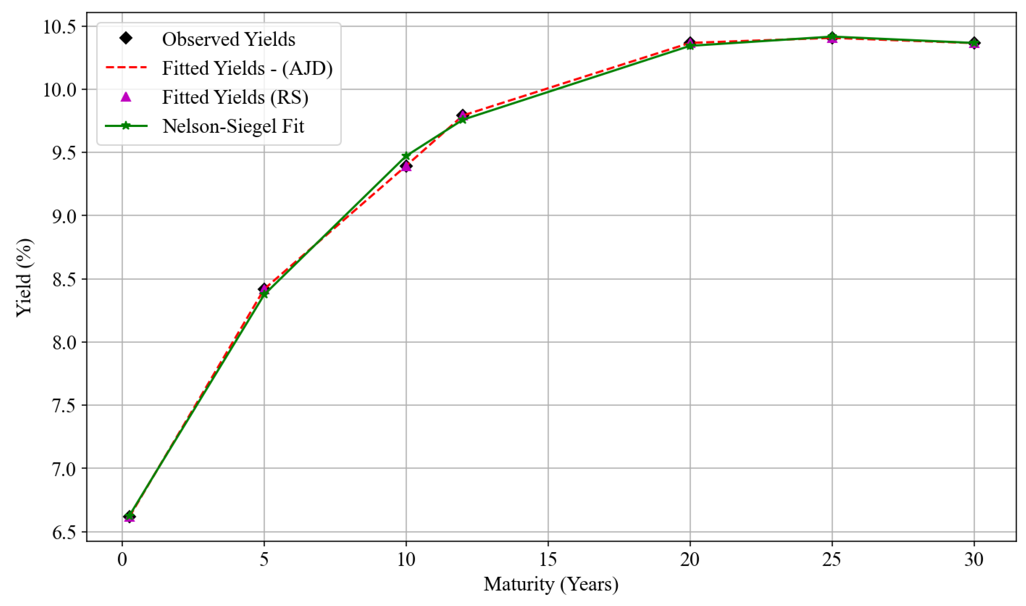
Figure 8 shows the average yield curves produced by each model. Both the AJD and RS-AJD models match the observed average yields nearly exactly at all maturities, demonstrating excellent cross-sectional fit. The Nelson-Siegel (NS) benchmark provides a comparably strong, though slightly less precise, fit. Time-series residuals for the AJD and RS-AJD models exhibit statistically significant autocorrelation, suggesting potential unmodeled dynamics. Another possibility emanates from the tension between the cross-section and time series of interest rates— possibly consistent with Unspanned Stochastic Volatility (USV) in the latent structure. Collin-Dufresne et al. (2009) highlight the issue of high autocorrelation which may imply model misspecification despite a reasonable unbiased yield fit exhibited by their model; see also Molibeli and van Vuuren (2025) for the USV and the tension between a cross-section and time series of interest rates. This gap motivates future work in extending the model with richer latent state dynamics and improved filtering.
Table 9 presents the in-sample and out-of-sample RMSEs (in basis points) for the AJD and RS-AJD models across various maturities. In-sample, the RS-AJD model provides slightly lower RMSEs at short and mid-term maturities, suggesting tighter fit. Out-of-sample RMSEs are higher than in-sample with AJD model exhibiting slightly lower RMSEs than RS-AJD.
Table 9.
In-sample and out-of-sample RMSE in basis points for the AJD and RS-AJD models across maturities. RS-AJD generally provides a better in-sample fit at short and medium maturities. Out-of-sample RMSEs are virtually identical across both models, indicating comparable forecasting performance.
Table 9.
In-sample and out-of-sample RMSE in basis points for the AJD and RS-AJD models across maturities. RS-AJD generally provides a better in-sample fit at short and medium maturities. Out-of-sample RMSEs are virtually identical across both models, indicating comparable forecasting performance.
| Maturity (Years) | In-Sample RMSE (bps) | Out-of-Sample RMSE (bps) | ||
|---|---|---|---|---|
| AJD Model | RS-AJD | AJD Model | RS-AJD | |
| 0.25 | 38.24 | 31.40 | 647.82 | 649.84 |
| 5 | 49.80 | 33.42 | 840.26 | 841.17 |
| 10 | 32.63 | 26.20 | 953.97 | 954.77 |
| 12 | 26.90 | 25.83 | 999.27 | 1000.05 |
| 20 | 25.59 | 26.63 | 1058.02 | 1058.80 |
| 25 | 25.53 | 25.70 | 1061.39 | 1062.12 |
| 30 | 25.12 | 24.85 | 1058.44 | 1059.18 |
8. Conclusion
In this study, jumps and regime-switching dynamics were introduced within the affine term structure framework to address the empirically observed non-normality in bond yields and their returns. The resulting models were calibrated using the UKF, and their performance was assessed through RMSE metrics, residual diagnostics, and visual inspection of fitted versus observed yield curves.
The inclusion of jumps and regimes was justified by a clear improvement in model fit, evidenced by lower in-sample and out-of-sample RMSE values and the model’s ability to reproduce key stylised facts, such as skewness and excess kurtosis. Residual diagnostics including Q-Q plots, autocorrelation, and distributional measures showed a movement toward Gaussianity, supporting the notion that the models capture critical nonlinearities and discontinuities in the yield process.
Some limitations remain. The assumption of a zero market price of risk may partially contribute to residual deviations from normality, particularly in the tails. The jump component was modeled using a simple Poisson process with constant intensity, and alternative Lévy-based jump processes—such as the variance gamma, normal inverse Gaussian, or Merton jump processes were not considered. Additionally, the marked point process was implemented through a kernel-compensated formulation, which, although analytically tractable, may not fully capture the complex jump dynamics observed in the data. Future work could explore these richer jump specifications to potentially improve model fit and better characterise the jump behavior.
Despite a strong post-calibration fit from both models, residuals exhibit statistically significant autocorrelation, suggesting missing dynamics. We hypothesise that this may be due to simplified jump modeling and fixed regime transitions. Inherent tensions between a cross-section and time series of interest ratses could be another possible cause for this misspecification. Future work could extend the framework to incorporate Lévy-type jumps and stochastic regime transitions, and employ advanced filtering methods —such as expectation maximasation (EM) and the Particle filter to improve state estimation.
Author Contributions
Conceptualization, M.M. and G.v.V.; methodology, G.v.V.; software, M.M.; validation, M.M., and G.v.V.; formal analysis, M.M., and G.v.V.; investigation, M.M. and G.v.V.; resources, M.M. and G.v.V.; data curation, M.M. and G.v.V.; writing—original draft preparation, M.M.; writing—review and editing, G.v.V.; visualization, M.M.; supervision, G.v.V.; project administration, G.v.V.; funding acquisition, None. All authors have read and agreed to the published version of the manuscript.
Funding
This research received no external funding.
Institutional Review Board Statement
Not applicable.
Informed Consent Statement
Not applicable.
Data Availability Statement
The data that support the findings of this study are available from the authors upon reasonable request.
Abbreviations
The following abbreviations are used in this manuscript:
| AJD | Affine Jump Diffusion |
| ATSM | Affine Term Structure Models |
| BIC | Bayesian Information Criterion |
| BDFS | Balduzzi P, Das SR, Foresi S |
| DM | Diebold–Mariano |
| DK | Duffie and Kahn |
| DTSM | Dynamic Term Structure Models |
| ODE | Ordinary Differential Equation |
| PCA | Principal Component Analysis |
| RMSE | Root-Mean-Square Error |
| RS-AJD | Regime Switching Affine Jump Diffusion |
| SA | South African |
| SME | Simulated Method of Estimation |
| SDE | Stochastic Differential Equation |
| SV | Stochastic Volatility |
| UKF | Unscented Kalman Filter |
| USV | Unspanned Stochastic Volatility |
Appendix A. Proof of Proposition 3
We prove the affine transform formula for the regime-switching affine jump diffusion (RS-AJD) model by constructing an exponential-affine martingale adapted to the joint process .
Fix and . Let be the mark space for jumps of X, and be the state space for Z.
Define deterministic functions for each regime :
to be specified as solutions to suitable generalized Riccati equations with terminal conditions:
Define the joint process:
Our goal is to show that is a local martingale with respect to the natural filtration generated by .
Recall the dynamics of and :
Here, is the compensated jump measure of X, and
with the compensated jump measure of Z.
Applying Itô’s formula and the product rule for jump processes:
Since and depend on regime which jumps, both parts contribute jumps. We decompose increments into:
- Continuous part from ,
- Jump part from ,
- Jump part from .
- (i) Continuous part from Xt
Using the SDE for in regime :
By Itô’s lemma (excluding jumps),
(ii) Jump part from Xt
The jump part contributes increments:
The exponential term changes by:
Hence, the compensated jump integral term in for is:
The predictable compensator contributes to the drift term:
(iii) Jump part from Zt
At a regime jump from to j, the process jumps by:
The increment is:
The compensated jump measure for is with compensator .
The predictable compensator term contributes to the drift:
To ensure is a local martingale (i.e., drift terms vanish), the functions , satisfy the generalised Riccati ODE system, for :
with terminal conditions:
Here, is the truncation function (e.g., ), is the affine volatility structure matrix, and the jump intensity function in regime i.
Conclusion
Under suitable integrability and regularity conditions, the process is a local martingale with
yielding the affine transform formula for the RS-AJD model.
Appendix B. UKF Algorithm
| Algorithm A1 Unscented Kalman Filter (UKF) for Affine Term Structure Models |
| Require: Initial state estimate , covariance , model parameters |
| 1: for each time step to T do |
| 2: Sigma Point Generation: |
| 3: Compute sigma points from , |
| 4: Prediction Step: |
| 5: for each sigma point do |
| 6: Propagate via transition function: |
| 7: end for |
| 8: Compute predicted mean: |
| 9: Compute predicted covariance: |
| 10: Update Step: |
| 11: for each sigma point do |
| 12: Map to observation space: |
| 13: end for |
| 14: Compute predicted measurement: |
| 15: Compute innovation covariance: |
| 16: Compute cross-covariance: |
| 17: Compute Kalman gain: |
| 18: Update state estimate: |
| 19: Update covariance: |
| 20: end for |
References
- Ang, Andrew and Geert Bekaert. 2002. Regime switches in interest rates. Journal of Business & Economic Statistics 20(2), 163–182. [CrossRef]
- Ang, Andrew and Allan Timmermann. 2012. Regime changes and financial markets. Annu. Rev. Financ. Econ. 4(1), 313–337. [CrossRef]
- Bandara, Wachi and Richard Munclinger. 2011. Term structure modeling with structural breaks: a simple arbitrage-free approach. Available at SSRN 1974033.
- Cheng, Guorui, Jingang Liu, Wenbo Zhang, and Shenmin Song. 2024. Gaussian filter estimation framework for nonlinear systems with multiple non-ideal scenarios. In 2024 36th Chinese Control and Decision Conference (CCDC), pp. 2793–2799. IEEE.
- Chourdakis, Kyriakos. 2002. Continuous time regime switching models and applications in estimating processes with stochastic volatility and jumps. U of London Queen Mary Economics Working Paper (464).
- Christoffersen, Peter, Christian Dorion, Kris Jacobs, and Lotfi Karoui. 2013. Nonlinear kalman filtering in affine term structure models: Internet appendix. Rotman School of Management Working Paper (2322760). [CrossRef]
- Collin-Dufresne, Pierre, Robert S Goldstein, and Christopher S Jones. 2009. Can interest rate volatility be extracted from the cross section of bond yields? Journal of Financial Economics 94(1), 47–66. [CrossRef]
- Cont, Rama. 2001. Empirical properties of asset returns: stylized facts and statistical issues. Quantitative Finance 1(2), 223. [CrossRef]
- Cont, Rama, Peter Tankov, and Ekaterina Voltchkova. 2004. Option Pricing Models with Jumps Integro-differential Equations and Inverse Problems. École polytechnique.
- Cox, John C, Jonathan E Ingersoll Jr, and Stephen A Ross. 1981. A re-examination of traditional hypotheses about the term structure of interest rates. The Journal of Finance 36(4), 769–799. [CrossRef]
- Dai, Qiang and Kenneth J Singleton. 2000. Specification analysis of affine term structure models. The Journal of Finance 55(5), 1943–1978. [CrossRef]
- Dai, Qiang, Kenneth J Singleton, and Wei Yang. 2007. Regime shifts in a dynamic term structure model of us treasury bond yields. The Review of Financial Studies 20(5), 1669–1706. [CrossRef]
- Dempster, MAH, Elena A Medova, Igor Osmolovskiy, and Philipp Ustinov. 2018. A practical robust long-term yield curve model. pp. 273–314.
- Deng, Wenying. 2023. A Gaussian-process Framework for Nonlinear Statistical Inference using Modern Machine Learning Models. Ph. D. thesis, Harvard University.
- Ding, Yi, Dimos Kambouroudis, and David G McMillan. 2025. Forecasting realised volatility using regime-switching models. International Review of Economics & Finance, 104171.
- Duffie, Darrell, Damir Filipovic, and Walter Schachermayer. 2002. Affine processes and application in finance. Technical report, National Bureau of Economic Research.
- Duffie, Darrell and Rui Kan. 1996a. A yield-factor model of interest rates. Mathematical Finance 6(4), 379–406. [CrossRef]
- Duffie, Darrell and Rui Kan. 1996b. A yield-factor model of interest rates. Mathematical Finance 6(4), 379–406. [CrossRef]
- Duffie, Darrell, Jun Pan, and Kenneth Singleton. 2000. Transform analysis and asset pricing for affine jump-diffusions. Econometrica 68(6), 1343–1376. [CrossRef]
- Elliot, Robert J and Tak-Kuen Siu. 2013. Affine jump-diffusions with regime switching: applications in finance. Applied Mathematical Finance 20(5), 385–418.
- Hamilton, James D. 1989. A new approach to the economic analysis of nonstationary time series and the business cycle. Econometrica: Journal of the Econometric Society, 357–384.
- Hirsa, Ali. 2024. Computational Methods in Finance. Chapman and Hall/CRC.
- Hu, Qiaozhi George. 2022. A markov regime switching model for asset allocation. Available at SSRN 4094459.
- Julier, Simon J and Jeffrey K Uhlmann. 1997. New extension of the kalman filter to nonlinear systems. In Signal processing, sensor fusion, and target recognition VI, Volume 3068, pp. 182–193. Spie.
- Keller-Ressel, Martin, Walter Schachermayer, and Josef Teichmann. 2011. Affine processes are regular. Probability Theory and Related Fields 151(3), 591–611. [CrossRef]
- Landen, Camilla. 2000. Bond pricing in a hidden markov model of the short rate. Finance and Stochastics 4(4), 371–389. [CrossRef]
- Liu, Xi, Badong Chen, Bin Xu, Zongze Wu, and Paul Honeine. 2017. Maximum correntropy unscented filter. International Journal of Systems Science 48(8), 1607–1615. [CrossRef]
- Lv, Weijun, Chang Liu, Yong Xu, Renquan Lu, and Ling Shi. 2025. Gaussian framework for nonlinear state estimation with stochastic event-trigger and packet losses. Automatica 175, 112220. [CrossRef]
- Molibeli, Malefane and Gary van Vuuren. 2025. Usv-affine models without derivatives: A bayesian time-series approach. Journal of Risk and Financial Management 18(7), 395. [CrossRef]
- Ornthanalai, Chayawat. 2014. Levy jump risk: Evidence from options and returns. Journal of Financial Economics 112(1), 69–90. [CrossRef]
- Piazzesi, Monika. 2000. Essays in monetary policy and asset pricing. stanford university.
- Piazzesi, Monika. 2010. Affine term structure models. In Handbook of Financial Econometrics: Tools and Techniques, pp. 691–766. Elsevier.
- Qin, Shanshan, Zhenni Tan, and Yuehua Wu. 2024. On robust estimation of hidden semi-markov regime-switching models. Annals of Operations Research 338(2), 1049–1081. [CrossRef]
- Rypdal, Kristoffer. 2018. Empirical growth models for the renewable energy sector. Advances in Geosciences 45, 35–44. [CrossRef]
- Singleton, Kenneth J. 2006. Empirical dynamic asset pricing: model specification and econometric assessment. Princeton University Press.
- Van Beek, Misha, Michel Mandjes, Peter Spreij, and Erik Winands. 2020. Regime switching affine processes with applications to finance. Finance and Stochastics 24(2), 309–333. [CrossRef]
- Vasicek, Oldrich. 1977. An equilibrium characterization of the term structure. Journal of Fnancial Economics 5(2), 177–188. [CrossRef]
- Wu, Linlin and Ying Zeng. 2004. Regime-switching affine term structure models. Journal of Fixed Income 14(3), 58–70.
- Zhu, Chao, George Yin, and Nicholas A Baran. 2015. Feynman–kac formulas for regime-switching jump diffusions and their applications. Stochastics An International Journal of Probability and Stochastic Processes 87(6), 1000–1032. [CrossRef]
| 1 | The term generator is used in two related but distinct senses: denotes the infinitesimal generator of the joint continuous-time Markov process , whereas Q refers to the generator matrix of the finite-state Markov chain . Both describe short-term transition behavior, but in different mathematical contexts. |
| 2 | This motivates our use of the UKF as a more flexible estimation strategy, especially in light of the nonlinearities and regime-dependent jump dynamics. See also Chourdakis (2002), who highlights the challenges in estimating affine models with jumps and regime-switching. Robust UKF variants such as the Generalized Maximum-likelihood UKF (GM-UKF) have also shown promise in mitigating non-Gaussian residuals, even outside finance (Liu et al. 2017), further reinforcing the UKF’s applicability in this context. |
| 3 | The local optimisation employed the L-BFGS-B algorithm from the scipy.optimize library, which supports limited-memory quasi-Newton updates under bound constraints. |
Figure 1.
Yield Surface: Weekly Government Bond Yields over Time and Maturities showing the evolution of the term structure across different maturities and time. Data consists of weekly observations from government bonds across seven maturities, covering the period from 2015 to 2024. Data source: Thomson Reuters
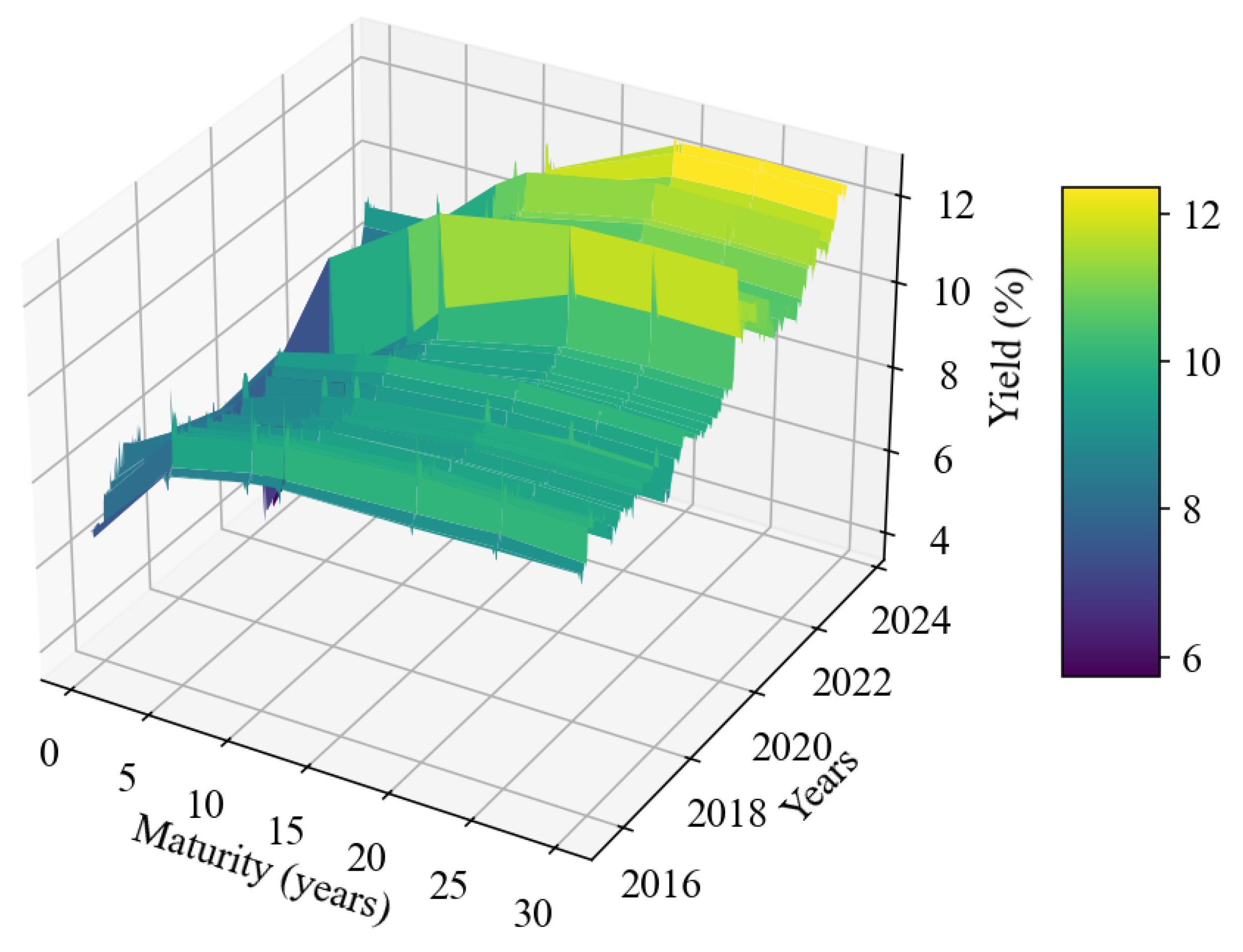
Figure 2.
PCA factors level, slope and curvature plotted over time in Years. AJD model fitted (reconstructed from UKF) Yields (%) are compared to the Observed Yields.
Figure 2.
PCA factors level, slope and curvature plotted over time in Years. AJD model fitted (reconstructed from UKF) Yields (%) are compared to the Observed Yields.
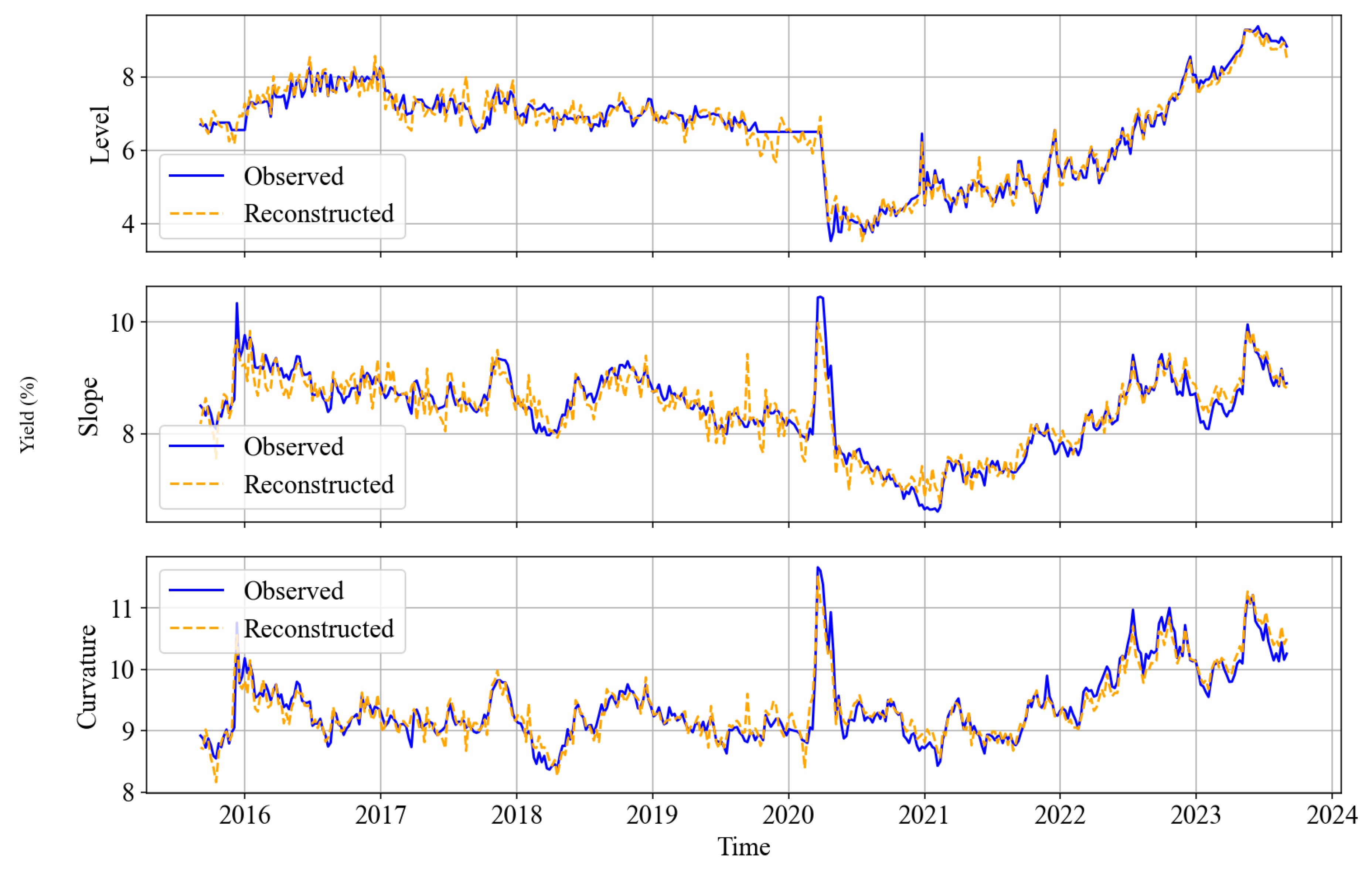
Figure 3.
Histograms and probability densties of AJD residuals. The probability densities are based on the Kernel density estimates (KDE) of the residuals for each PCA factor. Individual subplot represent the factors level, slope and curvture.
Figure 3.
Histograms and probability densties of AJD residuals. The probability densities are based on the Kernel density estimates (KDE) of the residuals for each PCA factor. Individual subplot represent the factors level, slope and curvture.
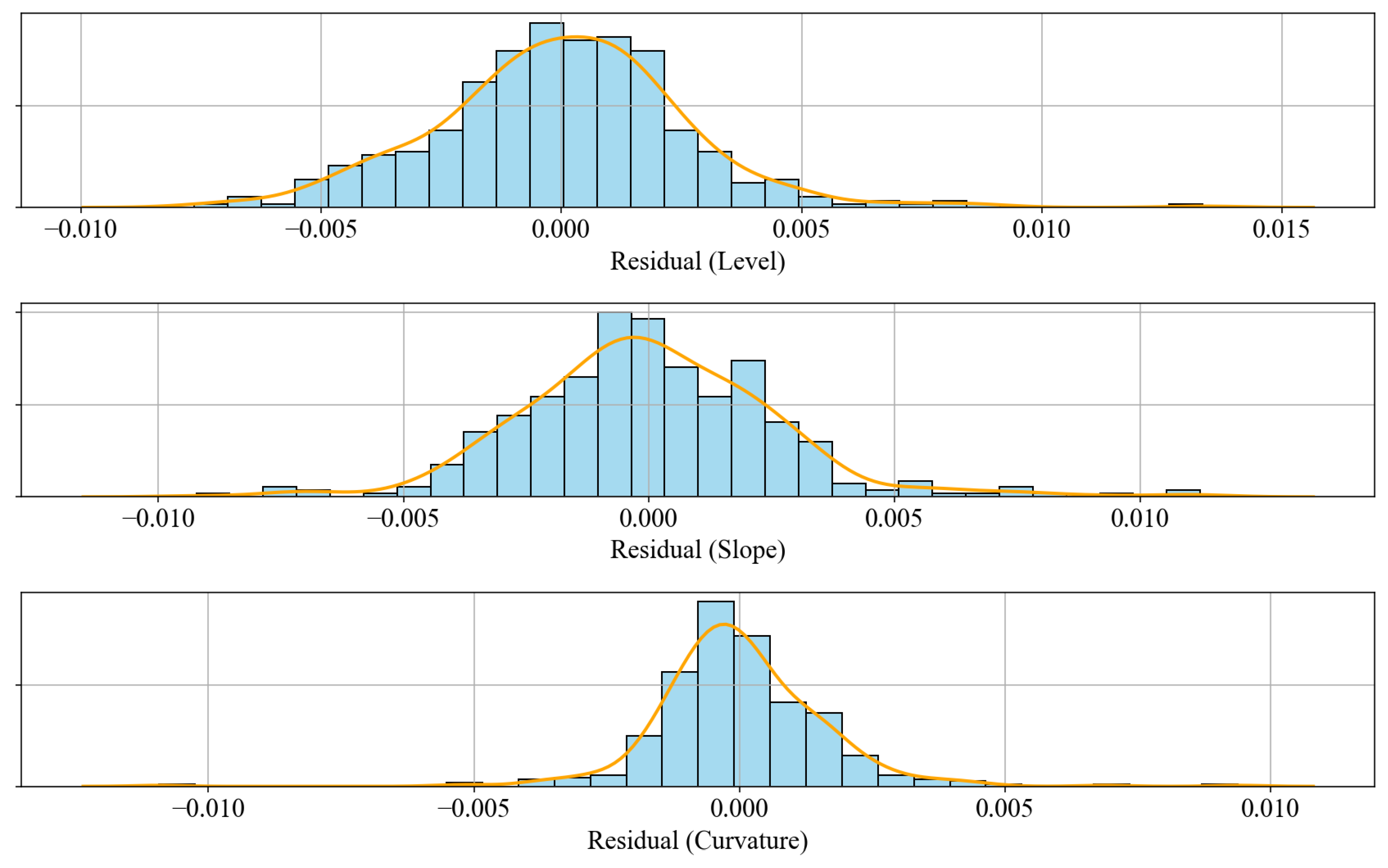
Figure 4.
QQ-Plots of AJD residuals for PCA components Level, Slope and Curvature. A blue line represents the actual observations while the red line theoretically implies symmetry about the mean and therefore normality. Any deviation from the red line may be indicative of a fat tail—skewness and kurtosis.
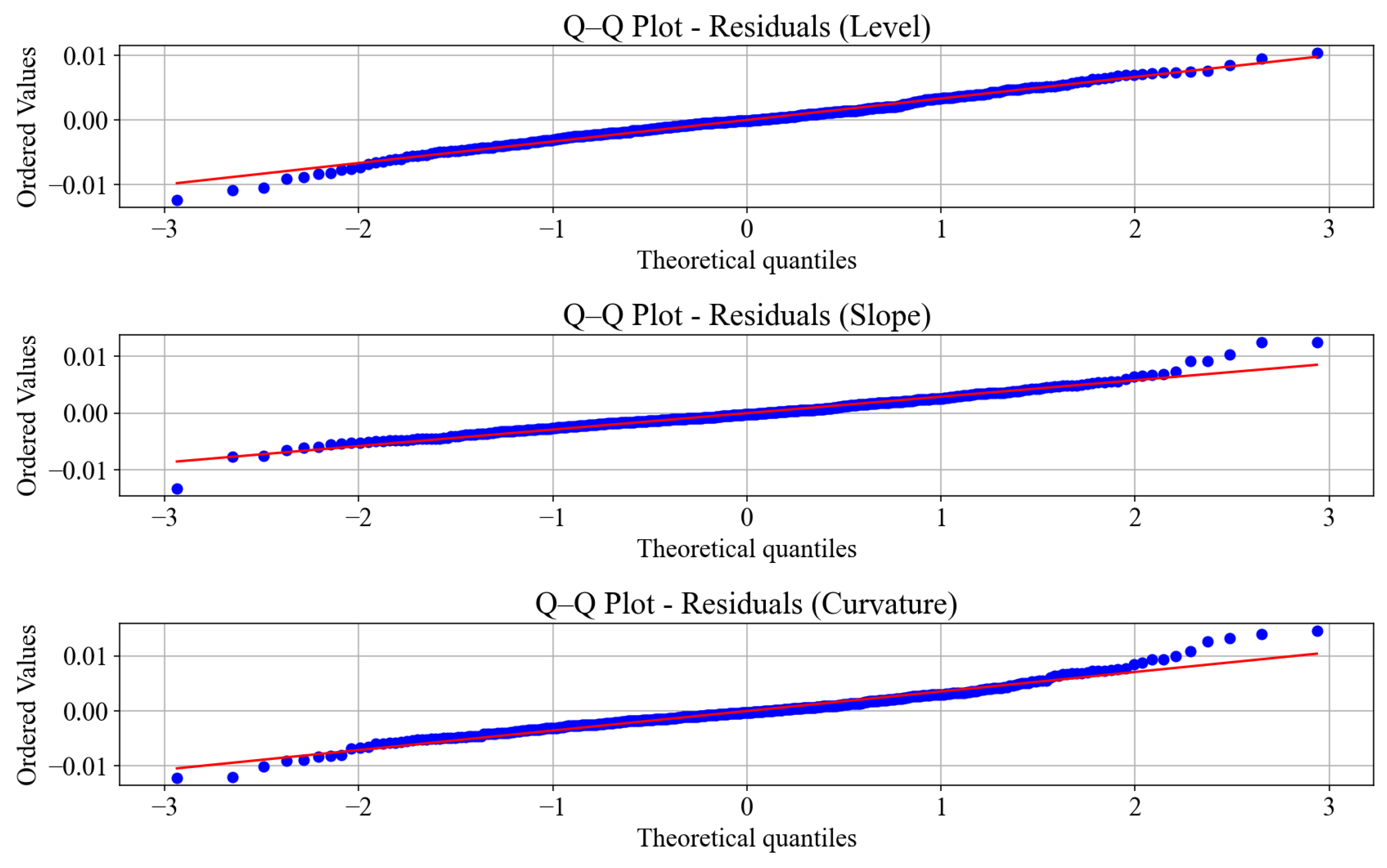
Figure 5.
PCA factors level, slope and curvature plotted over time in Years. The RS-AJD model fitted (reconstructed from UKF) Yields (%) are compared to the Observed Yields.
Figure 5.
PCA factors level, slope and curvature plotted over time in Years. The RS-AJD model fitted (reconstructed from UKF) Yields (%) are compared to the Observed Yields.
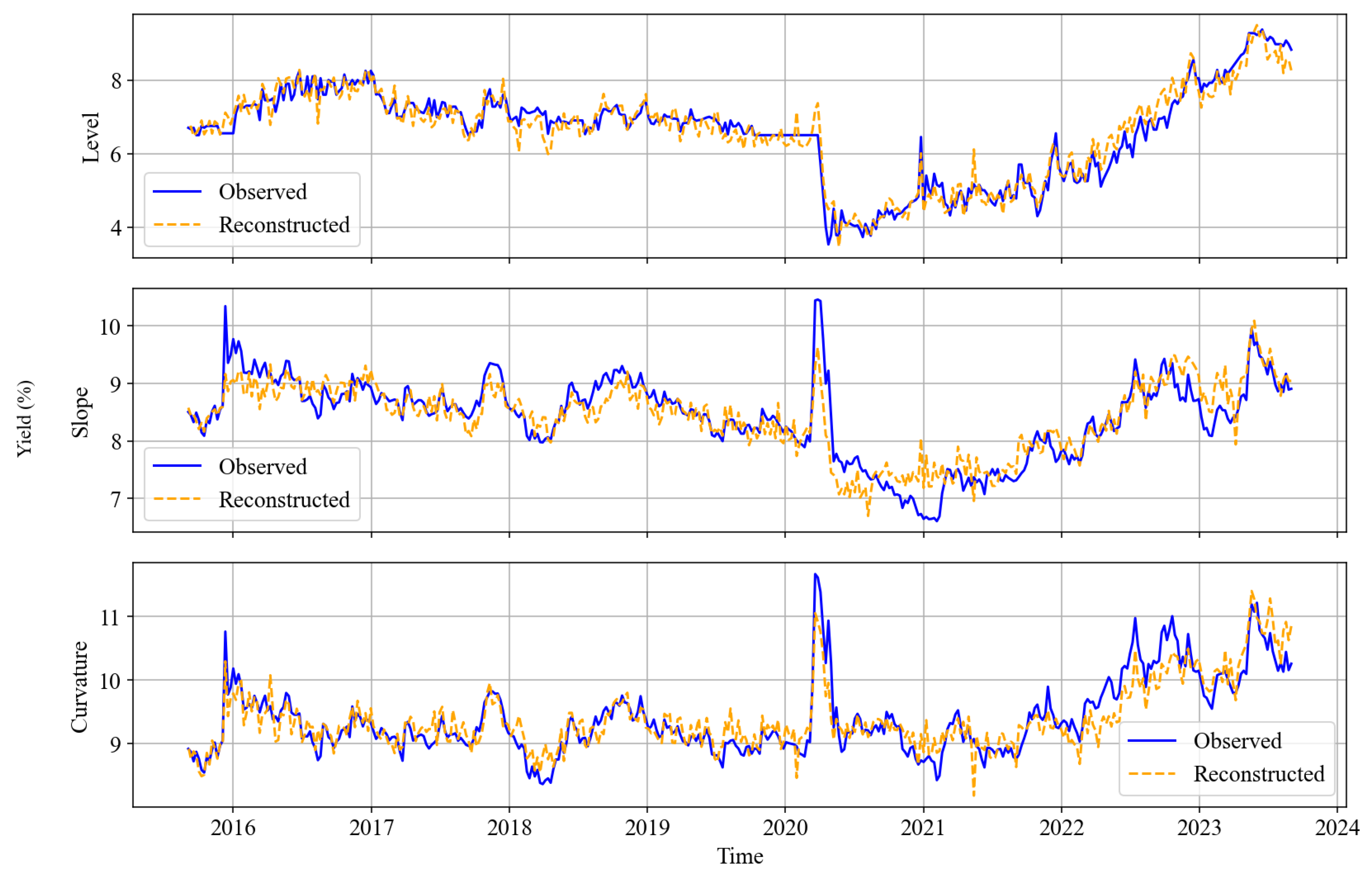
Figure 6.
Histograms and probability densties of RS-AJD residuals. The probability densities are based on the Kernel density estimates (KDE) of the residuals for each PCA factor. Individual subplot represent the factors level, slope and curvture.
Figure 6.
Histograms and probability densties of RS-AJD residuals. The probability densities are based on the Kernel density estimates (KDE) of the residuals for each PCA factor. Individual subplot represent the factors level, slope and curvture.
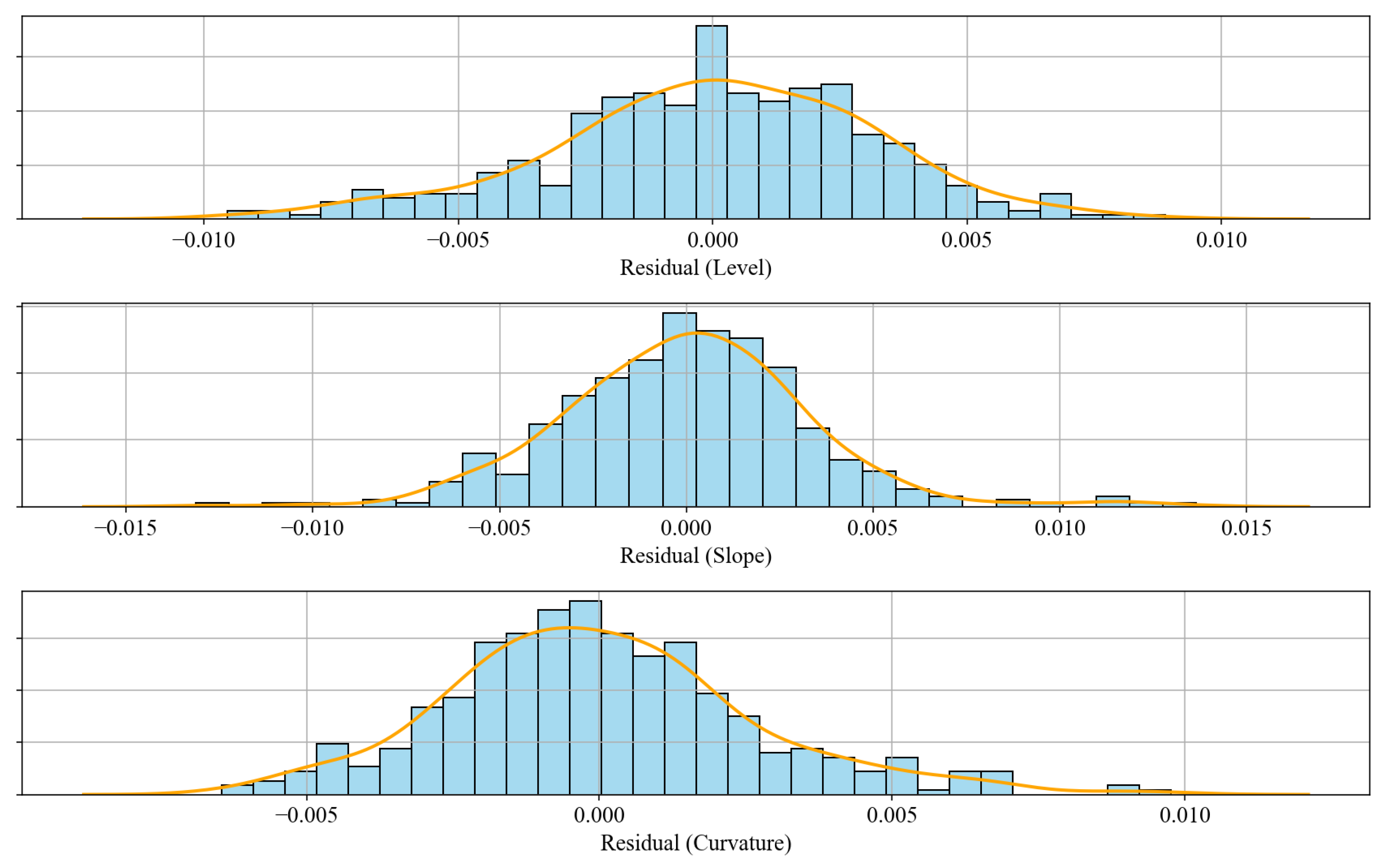
Figure 7.
QQ-Plots of RS-AJD residuals for PCA components Level, Slope and Curvature. A blue line represents the actual observations while the red line theoretically implies symmetry about the mean and therefore normality. Any deviation from the red line may be indicative of a fat tail—skewness and kurtosis.
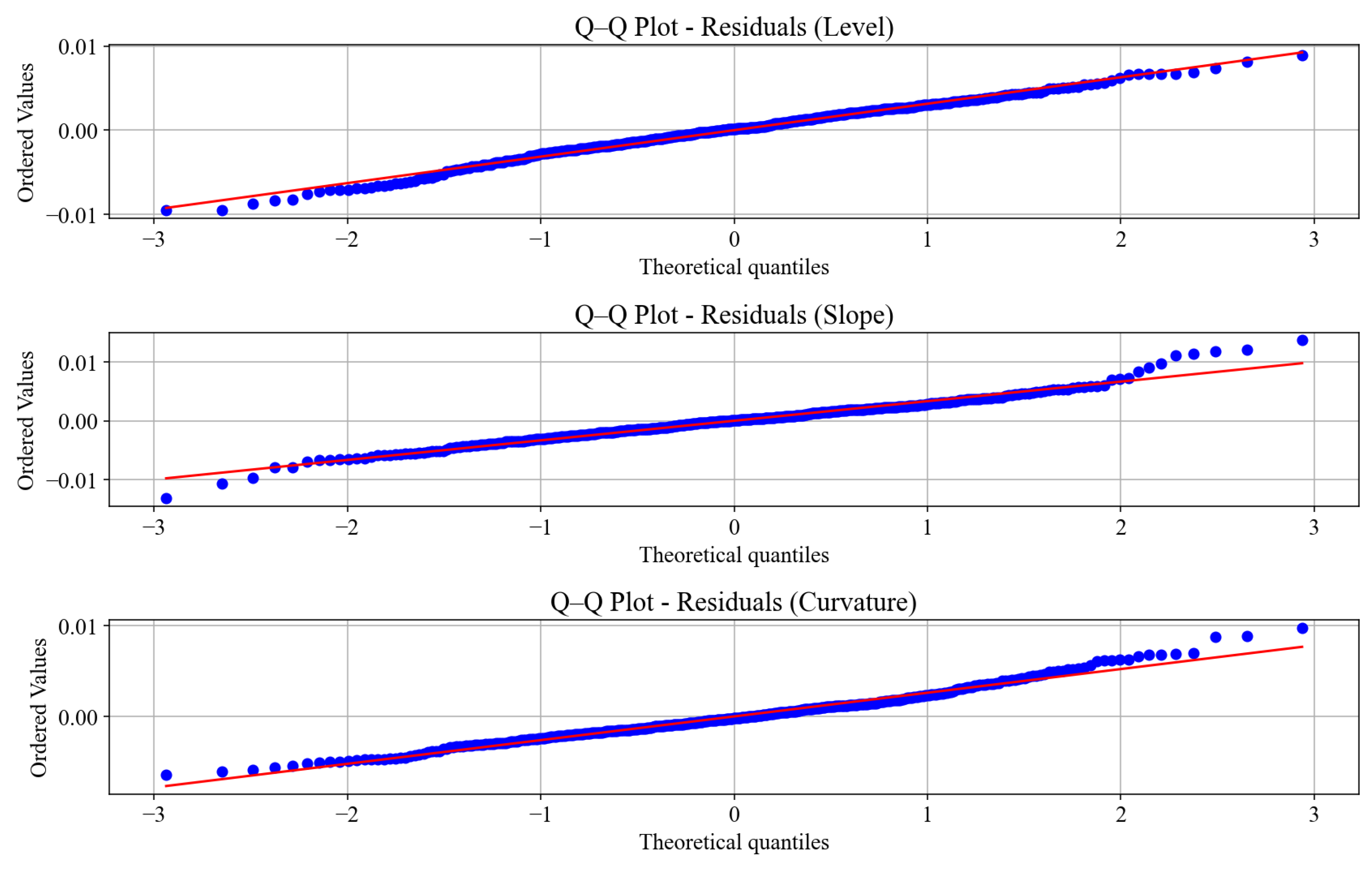
Figure 8.
Average yield curve across maturities. The AJD, RS-AJD, and NS models are calibrated to the same data. Both AJD and RS-AJD models perfectly fit the average yields, while the NS model shows minor deviations. The visual similarity across models demonstrates strong cross-sectional fit.
Figure 8.
Average yield curve across maturities. The AJD, RS-AJD, and NS models are calibrated to the same data. Both AJD and RS-AJD models perfectly fit the average yields, while the NS model shows minor deviations. The visual similarity across models demonstrates strong cross-sectional fit.
Disclaimer/Publisher’s Note: The statements, opinions and data contained in all publications are solely those of the individual author(s) and contributor(s) and not of MDPI and/or the editor(s). MDPI and/or the editor(s) disclaim responsibility for any injury to people or property resulting from any ideas, methods, instructions or products referred to in the content. |
© 2025 by the authors. Licensee MDPI, Basel, Switzerland. This article is an open access article distributed under the terms and conditions of the Creative Commons Attribution (CC BY) license (http://creativecommons.org/licenses/by/4.0/).
Copyright: This open access article is published under a Creative Commons CC BY 4.0 license, which permit the free download, distribution, and reuse, provided that the author and preprint are cited in any reuse.


