
Submitted:
11 August 2025
Posted:
12 August 2025
You are already at the latest version
Abstract
The Kennedy model provides a flexible and mathematically consistent framework for modeling the term structure of interest rates, leveraging Gaussian random fields to capture the dynamics of forward rates. Building upon our earlier work, where we developed both theoretical results — including novel proofs of the martingale property, connections between the Kennedy and HJM frameworks, and parameter estimation theory — and practical calibration methods, using maximum likelihood, Radon–Nikodym derivatives, and numerical optimization (stochastic gradient descent) on simulated and real par swap rate data, this study extends the analysis in several directions. We derive detailed formulas for the implied volatilities implied by the Kennedy model and investigate their asymptotic properties. A comprehensive sensitivity analysis is conducted to evaluate the impact of key parameters on derivative prices. We develop a Monte Carlo simulation scheme tailored to the conditional distribution of the Kennedy field, enabling efficient scenario generation consistent with observed initial forward curves. Furthermore, we present closed-form pricing formulas for various interest rate derivatives, including zero-coupon bonds, caplets, floorlets, swaplets, and the par swap rate, expressed explicitly in terms of the initial curve. Finally, we calibrate the Kennedy model to market-observed caplet prices. The findings provide valuable insights into the practical applicability and robustness of the Kennedy model in real-world financial markets.
Keywords:
Kennedy model
; calibration
; term structure model
; option pricing
; interest rate caplet
; Gaussian random field
; implied volatility
; sensitivity analysis
; caplet calibration
1. Introduction
In the last decade, the occurrence of negative interest rates has posed significant challenges for classical term structure models, motivating the development and re-evaluation of interest rate models capable of handling such phenomena. Among these, the Kennedy model, which describes forward rate dynamics as a Gaussian random field, offers a flexible framework that naturally accommodates negative rates while remaining consistent with the Heath–Jarrow–Morton (HJM) framework [1,4,6].
Building on our previous work [5], where we developed both theoretical results — including novel proofs of the martingale property, connections between the Kennedy and HJM frameworks, and parameter estimation theory — and practical calibration methods on par swap rates, using maximum likelihood, Radon–Nikodym derivatives, and numerical optimization (stochastic gradient descent) on simulated and real par swap rate data, this paper presents an extended analysis focusing on additional theoretical and practical aspects of the model. In particular, we explore implied volatilities, sensitivities, simulation techniques, and the calibration of the model to caplet prices using market-implied volatilities. We also analyze conditional expectations arising in the pricing formulas, which play a crucial role in evaluating interest rate derivatives.
The paper is organized as follows. Section 2 introduces the Kennedy model, its Gaussian random field structure, and the theoretical properties necessary for pricing interest rate derivatives [1]. We also discuss the special case where the model parameters and coincide, which leads to simplified formulas. Section 3 derives the conditional expectations and variances of key quantities, enabling pricing formulas that depend explicitly on the observed initial forward curve.
Section 4 describes a Monte Carlo simulation scheme adapted to the conditional distribution of the Kennedy field, while Section 5 presents the pricing formulas for various financial instruments, including zero-coupon bonds, caplets, floorlets, swaplets, and the par swap rate. Section 7 examines the sensitivity of model prices to changes in the parameters, providing insights into the model’s stability and robustness. Section 8 explores the relationship between the Kennedy model and the Black model, deriving implied volatilities analytically and investigating their asymptotic properties. Section 9 discusses the calibration of the Kennedy model to caplet prices based on market data, and evaluates both in-sample and out-of-sample performance.
We conclude the paper with a summary of findings and remarks on possible directions for future research.
2. Kennedy Model
The development of the forward rates in the model proposed by Kennedy is described in the upcoming equation.
where is a centered Gaussian random field with the covariance structure specified by
The function c is given and satisfies . We assume that the drift function is deterministic and continuous for , and the initial term structure of is specified. Additionally, we also have for . The covariance function is symmetric in and , and it is nonnegative definite in pairs and . The dependence on ensures that the Gaussian random field exhibits independent increments.
A sufficient condition for the drift surface is established to guarantee that the discounted zero-coupon bond prices are martingales. Therefore, the model can be used to price financial products in the future.
First, let us introduce the following notations, where .
where denotes the spot rate at time t, represents the price at time s of a bond paying one unit at time . defines the discounted price of the previously defined bond at time 0, with the information available at time s captured in the -algebra, indicating that the entire yield curve is observable at each time point. We also introduce a new notation, , for the continuously compounded forward rate over the interval ), which can be interpreted as an average of the forward rate for the current period, at time s.
An important theorem is emphasized in Kennedy’s article, which states the following [4].
Theorem 1.
In the independent-increments case the following statements are equivalent:
- (a)
- The discounted bond-price process is a martingale for each ;
- (b)
- , for all ; and
- (c)
- for all , .
The proof of the theorem is accessible in the original article written by Kennedy [1]. Furthermore, a different derivation of the theorem can be found in our previous article [5].
Assuming martingale property of the discounted bond price process, as well as stationarity and Markovianity of the forward rate field, the Kennedy model can be expressed in a closed form with four parameters . Under these assumptions, the covariance function of the forward rates takes the form
where , , and .
The martingale property is ensured by the drift term .
where is determined by the initial forward curve.
A detailed derivation of these results and a discussion of the underlying assumptions can be found in Kennedy’s original article [4] and in our previous work [5].
2.1. The Case
In this subsection, we investigate the special case of the Kennedy model when the two exponential decay parameters coincide, that is, when . In this setting, the analytical expressions of the covariance and the drift function significantly simplify, providing further insight into the internal structure of the model.
We begin by recalling the original covariance formula from equation (8), which is given by
When , the formula simplifies to
This simplified version exhibits a more symmetric structure and leads to a more tractable analytical form for pricing and simulation purposes.
The drift function originally given in equation (9) becomes undefined when due to a division by zero. However, by taking the appropriate limit, we obtain the well-defined expression
This formula remains continuous and well-behaved as and thus ensures a valid definition for the drift surface in the degenerate case.
Alternatively, one can derive the same formula using Theorem 1, part c, which expresses the drift surface in terms of the covariance function as
When using the simplified covariance formula for the case , this expression also yields the same drift surface as the one obtained from the limit calculation. The consistency of these two approaches confirms the analytical soundness of the model.
In conclusion, both derivations lead to the same expression for the drift surface, demonstrating that the Kennedy model remains internally consistent and mathematically stable even in the special case where .
3. Conditional Expected Value and Standard Deviation of and
In interest rate markets, the initial forward curve is directly observable from market data, and thus represents a valuable source of information for model calibration. Incorporating this observable curve into the modeling framework can significantly improve calibration accuracy, as it allows the model to be explicitly conditioned on information available at time zero. To this end, we derive the conditional expected values, variances, and correlations of the forward rates (and of their integrals over different timescales) given the observed initial forward curve. These quantities play a central role in the pricing of various interest rate derivatives.
Specifically, we introduce two integral quantities, consistent with our previous study, which capture the accumulation of forward rates over different time ranges:
By expressing these quantities as functions of the observed initial forward curve, we obtain pricing formulas that are consistent with market practice and more accurately aligned with the available information at the time of pricing. This, in turn, enhances the practical applicability of the model and its relevance for real-world calibration tasks.
Let be the -algebra defined by . Thus, the conditional expected value and variance of the terms in the pricing formula are as follows:
Therefore, we have to calculate the following expressions: , , and .
Let . It is known that the expression is independent of for all . In this case, we need to write down the covariance between the two and choose X such that, due to the properties of the normal distribution, it exactly cancels it out. Based on the previous results, using the covariance function of the special case Kennedy field, the following can be calculated:
Thus, we can conclude that if X is represented in the following form , then the covariance will be canceled out. Furthermore, we know that the expected value of the expression must be equal to , so X will be equal to the following expression, where in line with the previous notations.
In this case, the expected value will be equal to , and the covariance of the difference will be zero, thus we have shown that the conditional expected value will be equal to X, therefore
Then, transitioning to the conditional expected values of and
In the Gaussian case, the conditional variances are equal to the ordinary variances, hence as a result
Thus, in order to write the pricing formulas as a function of the initial forward curve, , we only need to calculate the conditional correlation between and , for which we first need to express the conditional covariance.
In the case of the Kennedy field, the conditional covariance is calculated as follows due to the properties of the correlation of the normal distribution.
Therefore, the conditional covariance of and is
First, we demonstrate the calculation of the first term.
Similarly to the first term, the calculation of the second part is demonstrated below.
By adding the two terms back together, we got the conditional covariance of and .
Based on this, we can conclude that the conditional correlation between and is equal to the conditional covariance divided by the standard deviations of and .
3.1. The case
In the special case where , we revisit the previously derived conditional expected values of and . In these expressions, the denominators involving become singular, so we apply first-order Taylor expansions and L’Hospital’s rule to evaluate the limits [12]. After simplification, we obtain the following results:
These simplified expressions show that in the limit case , the conditional expected values remain well-defined and retain a clear dependence on the initial forward curve and the exponential decay parameter .
When , the general formulas for the conditional variances contain singularities due to terms involving in the denominator, similarly to the conditional expected values. To resolve this, we apply L’Hospital’s rule and first-order Taylor expansions to obtain the limiting values. The resulting expressions are the following:
These results show that the conditional variance of remains unchanged, while the expression for the variance of simplifies to an explicit and finite formula in the degenerate case.
Similarly to the previous expressions, the general formula for the conditional covariance of and becomes singular as . To compute the limiting form, we apply L’Hospital’s rule and Taylor expansions term by term. After simplification, we obtain the following closed-form expression:
This expression is smooth and free from singularities, and can thus be used directly in the pricing formulas when .
4. Simulation
Since we have calculated the expected value and variance of the forward field conditional on the -algebra , the simulation process also needed to be revised compared to our previous study [5,9]. Our objective was to generate a Kennedy field based on a given initial forward curve input vector, ensuring that the field evolves according to the Kennedy model starting from the initial curve. Thus, let us denote the conditional expected value of the forward field with
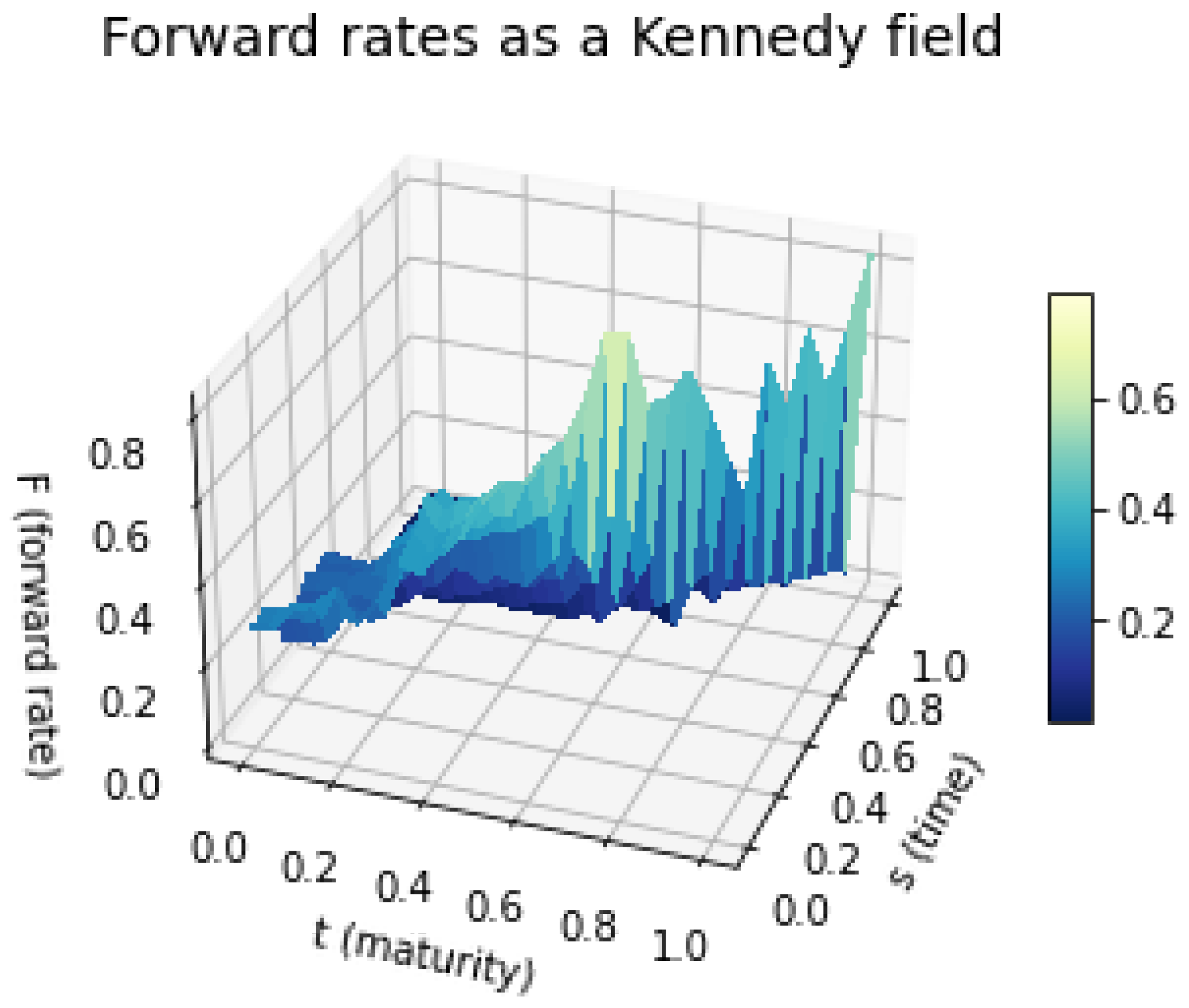
Similarly to the previous simulation, we first generate a Brownian sheet over an equidistant grid. Next, we apply an affine transformation by adding the conditional expected value to the generated sheet. By evaluating the field at the specified points, we obtain the Kennedy field, which matches the conditional expected value and variance as prescribed [8]. Therefore, produces the desired Kennedy field.
Figure 1.
Conditional simulation of the Kennedy forward–rate field , using parameters calibrated to the April 2025 USD caplet panel and conditioning on the observed initial forward curve for that month.
Figure 1.
Conditional simulation of the Kennedy forward–rate field , using parameters calibrated to the April 2025 USD caplet panel and conditioning on the observed initial forward curve for that month.
5. Pricing Formulas
In the following section, we will write the previously derived pricing formulas using conditional expected values, variances, and covariance, which will make the formulas dependent on the initial forward curve. As a result, there will be additional information incorporated into the formulas.
Let us start with one of the simplest financial product, the zero coupon bond which pays 1 at time t. Therefore, the price of the zero coupon bond calculates as follows.
Based on the above, the price of a zero-coupon bond can be calculated in two ways. First, by simulating the forward field and subsequently using Monte Carlo simulation to estimate the price of the financial product. Alternatively, it can be derived by substituting the original parameters in the previously calculated conditional expected value.
Compared to the pricing formulas derived in our earlier work [5], the general structure of the caplet, floorlet, and swaplet prices remains unchanged. However, in the current formulation, the unconditional expectations, variances, and correlations appearing in those formulas are replaced by their conditional counterparts, explicitly conditioned on the observed initial forward curve. This modification allows the pricing formulas to remain analytically tractable while making them more consistent with the information available in the market at time zero. As a result, the model becomes more aligned with practice, enabling more accurate calibration and interpretation of the implied prices.
In our earlier work, the parameters of the Kennedy model were calibrated to observed par swap rate data, utilizing the explicit pricing formula for the par swap rate in the unconditional setting. In the present study, we extend this analysis by deriving the par swap rate also under the assumption that the initial forward curve is observed and fixed. This conditional formulation preserves the tractability of the pricing formula, while making it more consistent with market practice and better suited for calibration to real-world data. The covariance function simplifies in this setting to the expression below, reflecting the fact that the entire yield curve at time zero is incorporated into the model.
From this, the par swap rate in the Kennedy model takes the following form:
6. Monte Carlo Simulations
To validate the correctness of the analytical pricing formulas derived earlier, we perform Monte Carlo simulations [7]. The key idea of this approach is to simulate a large number of realizations of the forward rate field using the simulation algorithm presented in Section 4. For each simulated path, we compute the corresponding payoffs of the financial products under consideration. As the number of simulation runs tends to infinity, the average simulated price converges to the theoretical price implied by the model. This provides a robust numerical check on the analytical results, ensuring consistency between the theoretical derivations and the stochastic dynamics of the model.
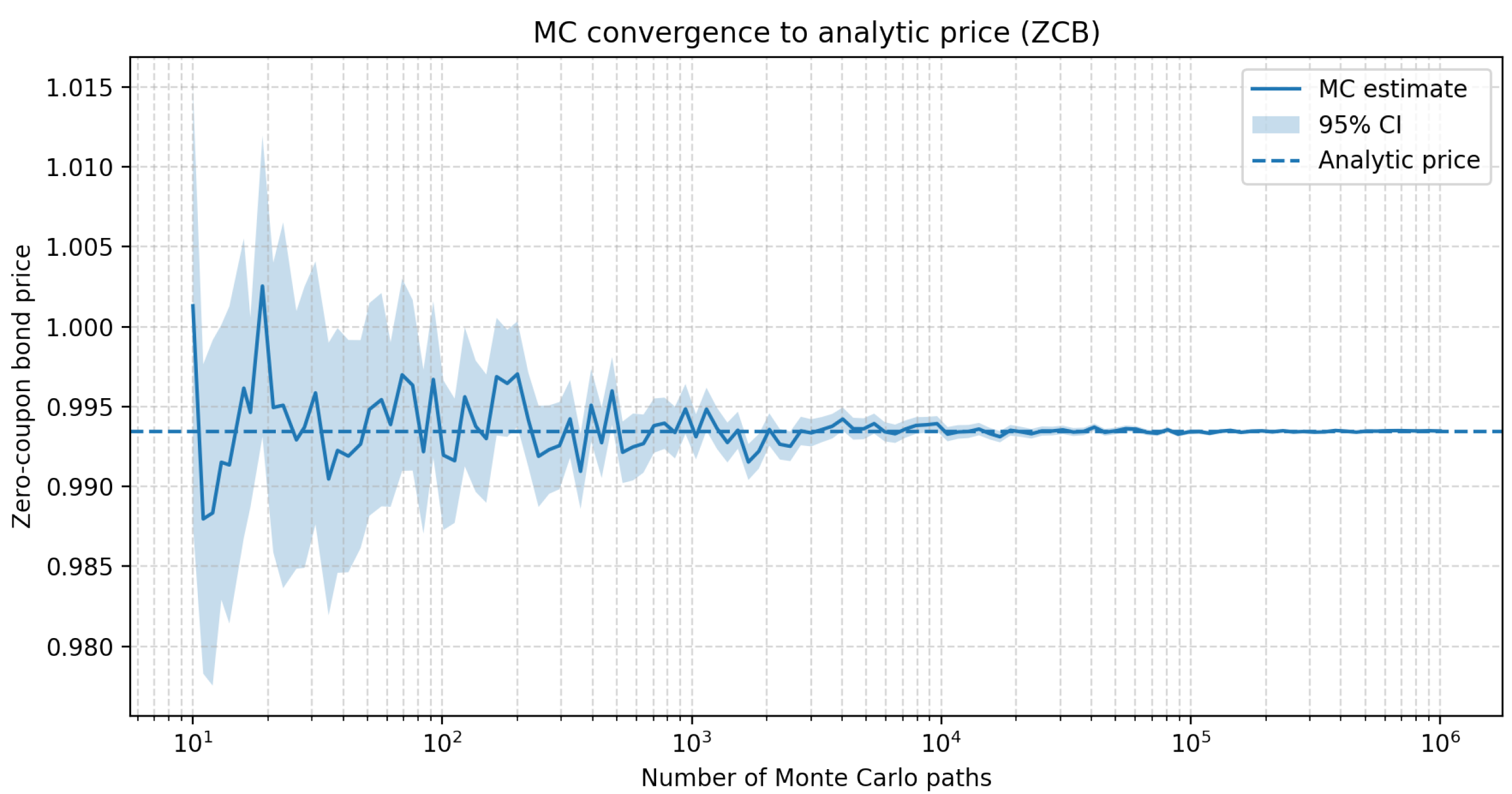
The figure below plots the Monte Carlo estimate of the zero-coupon bond price as a function of the number of simulated paths on a log scale. The dashed horizontal line shows the closed-form price, the solid curve is the Monte Carlo mean, and the shaded band is the pointwise 95% confidence interval. As the number of paths increases, the Monte Carlo estimate stabilizes and the confidence band shrinks, converging to the analytic benchmark.
Figure 2.
Monte Carlo convergence to the analytical zero-coupon bond price in the Kennedy model
Beyond serving as a validation tool, Monte Carlo simulation also offers practical advantages when pricing more complex derivatives, for which closed-form solutions may not be available. In particular, the flexibility of the simulation framework allows us to incorporate path-dependent features, non-standard payoff structures, or alternative assumptions about the forward curve. However, this comes at the cost of increased computational burden: achieving high accuracy requires a large number of simulation runs, which can be time-consuming.
7. Sensitivity Analysis
In this section, we conduct a sensitivity analysis on the prices of the financial instruments introduced earlier, including zero coupon bond, caplet and swaption. The aim is to examine how the values of these derivatives respond to changes in the key model parameters. By systematically varying the input parameters—such as the volatility , the mean-reversion speed , and the long-term mean — we assess the robustness of the pricing formulas and the overall behavior of the model. This analysis provides valuable insight into the model’s stability and practical applicability in real market conditions.
For the zero coupon bond and caplet, we carry out the sensitivity analysis using both the analytical pricing formulas and Monte Carlo simulations, allowing us to compare the efficiency and consistency of the two approaches. In contrast, for the swaption, due to the lack of a closed-form pricing formula, the sensitivity analysis is performed solely via Monte Carlo simulation.
We examine the sensitivity of both caplet and swaption prices to changes in the parameters of the Kennedy model. Caplet pricing is carried out using analytical formulas, while swaption prices are derived via Monte Carlo simulation. The model parameters under investigation include the drift , the long-term mean level , the volatility , and the decay parameter . We also consider the effect of observable market inputs, such as the strike rate K and the time to maturity T.
To measure how price changes with respect to a given parameter, we apply a central finite-difference approximation of the partial derivative. These numerical approximations are analogous to the Greeks in the Black-Scholes framework [11]. For a parameter , we compute a discrete sensitivity as
where denotes price of a financial asset evaluated at the perturbed value of the parameter and is a small increment, typically . These derivatives approximate how robust the model output is to perturbations in the parameters obtained during calibration.
Figure 3 presents the sensitivity results for the caplet prices. The plots reveal that increasing the maturity T results in lower caplet prices, reflecting the lower present value of longer-dated claims. When the strike rate K increases, the caplet becomes less valuable due to reduced intrinsic value. As the volatility increases, the caplet price grows sharply, displaying strong convexity and indicating significant vega sensitivity. Variations in and lead to more nuanced effects: the response is generally non-monotonic and reflects the delicate interaction between mean reversion and discounting within the forward rate field.
Figure 4 illustrates the analogous sensitivity for swaption prices, obtained via numerical simulation. In contrast to caplets, swaption values increase with maturity, owing to the cumulative optionality embedded in longer-term swap contracts. Increasing the strike rate reduces swaption prices approximately linearly over the observed range. Volatility has a pronounced convex impact on swaption prices, underscoring the importance of accurately estimating . The long-term mean also plays a key role; as it increases, the forward curve shifts upward, thereby increasing the value of the option. On the other hand, changes in the drift lead to a decreasing trend in the price, while the response to is more erratic and displays non-monotonic behavior.
These results underline the relative importance of the various model parameters. Volatility clearly has the largest impact on both caplet and swaption pricing, making its accurate calibration critical for effective risk management and valuation. The mean reversion level has a notable effect particularly for long-dated instruments, as it governs the average level of the forward rate over time. The drift parameter and decay parameter influence the curvature and decay dynamics of the forward curve, and although their impact is less direct, they remain essential for fine-tuning model behavior.
From a calibration perspective, the results suggest a possible hierarchical approach: one may first calibrate and , which dominate price level sensitivity, and then refine and to better match the forward curve’s shape and dynamics.
8. Implied Volatility
In practice, option prices are often quoted in terms of implied volatilities rather than direct prices. Therefore, it is natural and useful to transform the model prices into implied volatilities, which can be computed either under the assumption of a lognormal distribution (as in the Black-model) or a normal distribution (as in the Bachelier model). Expressing prices in terms of implied volatilities has several advantages. First, it aligns the model output with market conventions, facilitating direct comparison with observed quotes. Second, the calibration surface expressed in implied volatilities tends to be smoother and more stable than the surface of prices, which improves numerical stability during calibration. Finally, working with implied volatilities allows us to assess the model’s ability to reproduce characteristic market patterns, such as the volatility smile or skew, which are directly observable in the implied volatility space [10].
8.1. Black Model
The Black model is an industry standard model in the pricing of European options written on forwards and futures [2]. The model assumes that the forward price of the underlying asset follows a lognormal distribution under the risk-neutral measure, which is consistent with the no-arbitrage pricing framework.
In this setting, the price of a European call option on a forward contract with forward price F, strike price K, time to maturity T, risk-free rate r, and volatility is given by:
where
Here, denotes the cumulative distribution function of the standard normal distribution. The term represents the standardized distance of the forward price from the strike, adjusted for volatility and time, while accounts for the expected downward drift due to the volatility over the remaining time to maturity.
In the context of interest rate derivatives, such as caplets and floorlets, the Black model is particularly relevant because these instruments can be viewed as options on forward rates. Under the Black framework, the forward rate is assumed to follow a lognormal process, and the price of a European caplet can be expressed in the same functional form as the above call option price. This allows practitioners to quote and compare caplet prices conveniently in terms of implied volatilities derived from the Black formula, aligning with market conventions.
This formulation provides a tractable and closed-form solution for option prices, facilitating calibration and interpretation in practice. In later sections, we will build on this framework to compare and align the Kennedy model with the Black model in order to analyze their respective implications for implied volatilities and pricing accuracy.
8.2. Comparison Between the Kennedy and Black Models
In this section, we aim to establish a direct correspondence between the Kennedy model and the Black model in order to derive a closed-form expression for the implied volatility implied by the Kennedy framework. By aligning the caplet pricing formulas of the two models, we can express the implied volatility as a function of the Kennedy model’s parameters. This is particularly useful because implied volatilities are the standard way of quoting option prices in financial markets, and having an analytical formula enables efficient calibration and better comparability with market data.
The price of a caplet in the Kennedy model is given by following expression
we align its structure with the Black model to express the implied volatility explicitly within the Kennedy framework.
Based on these considerations, the correspondence between the two models can be established as follows:
For verification, let us examine the quantities denoted by and :
Therefore, the Kennedy model can be perfectly aligned with the Black model, allowing for an analytical, closed-form expression for the implied volatility:
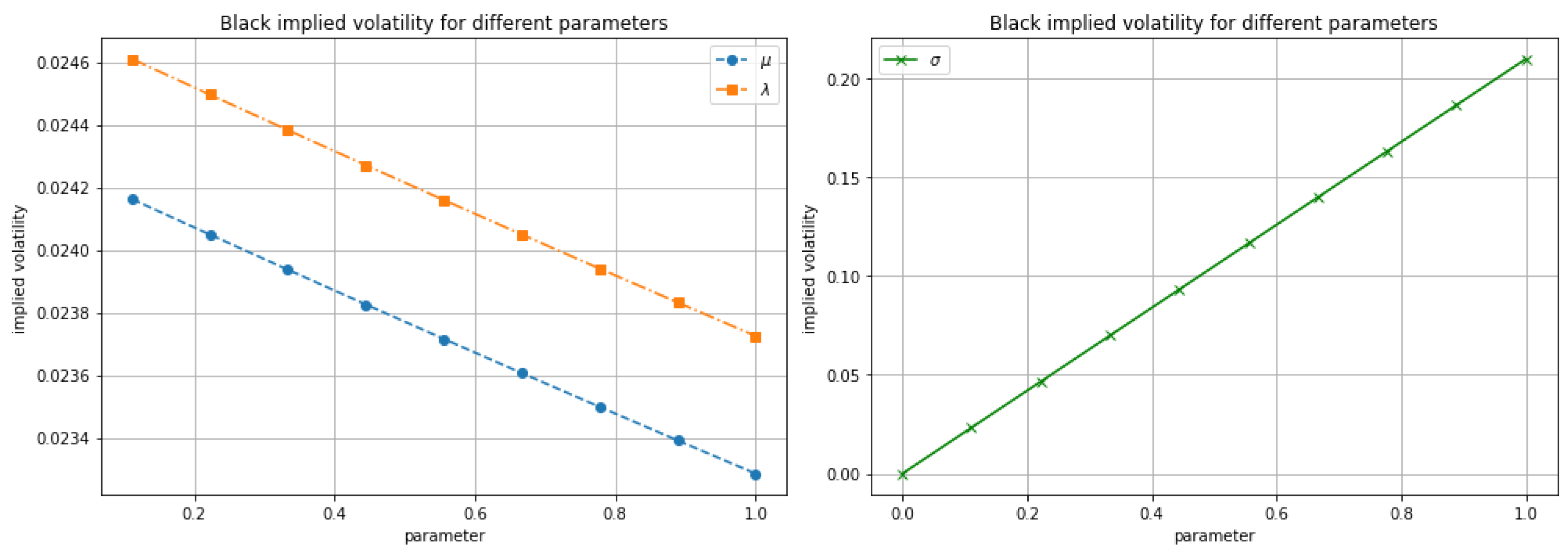
It can be observed that the strike price does not appear in the closed-form expression of implied volatility. Consequently, the implied volatility curve as a function of the strike price will be flat, and the model does not exhibit a volatility smile.
Figure 5.
The sensitivity of the implied volatility, backed out from the Black model, to various parameters.
Figure 5.
The sensitivity of the implied volatility, backed out from the Black model, to various parameters.
The limiting case when takes the following form:
We now examine the first- and second-order asymptotics of the implied volatility derived from the Black model, in the limit as approaches zero. Hence, the first-order expansion is:
The second-order expansion yields:
The implied volatility converges to this expression at second order. The Kennedy model assumes that , a condition which can also be justified by the second-order expansion, since the convergence rate must necessarily be positive. Therefore, the term is strictly positive. Consequently, .
This asymptotic behavior is relevant from both a theoretical and practical standpoint. The fact that the implied variance decays as for short maturities ensures that the Kennedy model remains well-behaved in the limit of small accrual periods, avoiding volatility spikes that may arise in other forward rate models. From a calibration perspective, this result implies that short-maturity caplets contribute only minimally to the total calibration error, which can improve numerical stability and reduce overfitting. Moreover, the positivity condition not only guarantees the correct convergence rate but also aligns with typical empirical parameter estimates observed in interest rate markets.
9. Calibration of the Kennedy Model to Caplet Prices
The data related to various financial instruments presented in this article were obtained from the Bloomberg Terminal. For each product, we collected transaction prices, corresponding normal implied volatilities, and at-the-money (ATM) strike levels, along with the relevant discount factors for present value calculations. The dataset covers USD-denominated interest rate derivatives, including caplets and swaptions, and was retrieved with monthly frequency from June 8, 2024, to April 8, 2025.
In this section, we describe the calibration of the Kennedy model to observed caplet prices. First, we calibrated the model to three-month caplets usin a numerical extremum search algorithm that relies on stochastic gradient descent and analytical pricing formulas.
The available dataset consists of European-style caplets and swaptions with single future payments. Each instrument is defined by two dates: the in date, indicating the beginning of the fixed leg (i.e., the payment time), and the for date, representing the tenor of the swap. Since these products involve only one payment, they can be treated as caplets with a three-month accrual period. For each instrument, the at-the-money strike rate (fixed rate) is also provided and used as the strike K in pricing.
The calibration procedure begins by constructing the initial forward rate curve from zero-coupon discount factors. This is done using the classical forward rate interpolation formula:
where denotes the zero-coupon bond price at time zero maturing at time t. The resulting forward curve serves as a deterministic input to the pricing model.
To determine the optimal parameters of the Kennedy model, we formulate the calibration as a numerical optimization problem. The objective function measures the discrepancy between model-implied and market-observed caplet prices, and is defined as a weighted sum of squared log-scale errors. Specifically, we minimize:
where is a maturity-dependent weight, assigning higher importance to longer maturities. The use of logarithmic error is motivated by the form of the Kennedy pricing formula, which contains multiple exponential terms. Working in log-space reduces the impact of large relative differences and improves numerical stability, particularly in regions where prices are small or highly sensitive to parameter changes.
To further improve robustness, a weak regularization term is added to the objective to prevent overfitting and to avoid implausible parameter values. Moreover, in order to better explore the parameter space and reduce the risk of convergence to local minima, the optimization is initialized from several different starting points, including randomly generated ones.
The optimization is carried out using the Sequential Least Squares Programming (SLSQP) algorithm, subject to box constraints and the structural condition , which ensures stationarity of the Gaussian field [3]. Additionally, all three model parameters (, , and ) are required to be strictly positive. The best solution among all starting points is selected based on the minimized error.
Following the optimization, we compute the model-implied caplet prices using the calibrated parameters, and assess the quality of the fit using average absolute and relative error metrics.
The calibration procedure described above is repeated independently for each month in an eleven-month historical window, from 2024 June to 2025 April. For each month, we extract the corresponding market data: the observed caplet prices, the associated at-the-money strike rates, and the initial forward rate curves. Each monthly dataset consists of caplets with a fixed accrual period months and seven different maturities: 3 months, 6 months, 1 year, 2 years, 5 years, 10 years, and 20 years.
Using the monthly data, the same optimization routine is applied to obtain a separate set of Kennedy model parameters for each month. This results in a time series of calibrated parameter triplets, allowing us to observe how the term structure dynamics evolve over time.
To assess the performance of the model, we compare the market-observed caplet prices with the model-implied prices calculated using the calibrated parameters. Figure 6 displays this comparison across all months. The fit is visually close for most maturities, and the monthly average relative errors are also computed to quantify accuracy.
The relative error between the calibrated (model-implied) caplet prices and the market-observed prices remains within the range of 5%–10% across all months considered. Such accuracy is generally regarded as indicative of a well-performing calibration.
Furthermore, the temporal evolution of the calibrated parameters is presented in Figure 7. These plots provide insight into how the forward curve’s volatility structure and mean reversion characteristics have changed over time, potentially reflecting macroeconomic developments or shifts in market sentiment.
As the plot of the Kennedy model parameters over time shows, the values of and tend to move closely together. This observation motivated an additional analysis, in which we examined how the model performs under the constraint , reducing the number of calibrated parameters from three to two. Our aim was to assess how much the model’s performance deteriorates when this structural simplification is imposed. We found that, in this case, the prices of the financial instruments become insensitive to the time parameter t, leading to a flat caplet price curve as a function of maturity. Consequently, this specification cannot be calibrated effectively.
Furthermore, since the parameter remains relatively stable throughout the observed time window, we also explored the impact of fixing to be constant across time, in order to evaluate whether such a simplification would still yield acceptable pricing accuracy. This aspect is subject to further research.
In addition to the calibration quality within each month, we also investigated the predictive performance of the model by evaluating how well parameters estimated in month t forecast caplet prices in month . For each month after the initial one, we computed caplet prices using the forward curve of the current month and the Kennedy parameters calibrated in the previous month. This allows us to assess the stability and forecasting power of the Kennedy model across time.
To visualize this, Figure 8 displays the market prices, the calibrated model prices using the current month’s parameters, and the forecasted prices using the previous month’s parameters. The figure includes twelve subplots, one for each month, along with the average relative errors for both the fitted and forecasted prices. The results demonstrate that while the Kennedy model fits the observed prices well in-sample, the forecasting performance is slightly worse but still remains within an acceptable error margin.
In this case, the relative error exhibits greater dispersion, ranging between 6% and 15%. Nevertheless, such accuracy can still be regarded as indicative of a reasonably good forecasting performance.
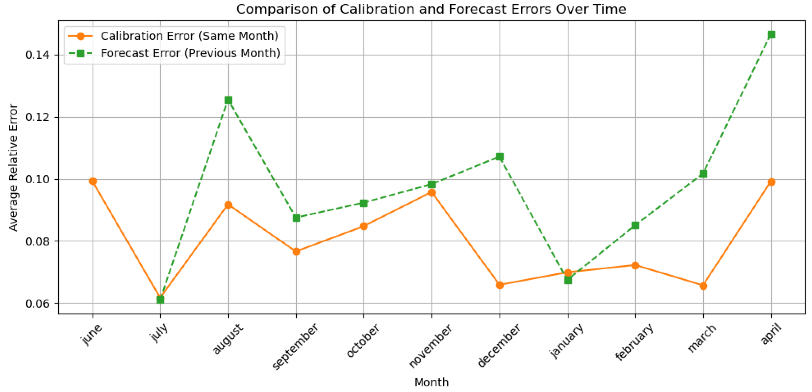
To summarize the difference between in-sample and forecast performance, Figure 9 plots the time series of average relative errors for both the calibrated model and the forecasted prices. This comparison helps evaluate how well the Kennedy model generalizes across time when parameter updates are delayed.
10. Discussion
Conditioning the Kennedy field on the observed initial forward curve proved useful both conceptually and empirically. The closed-form conditional moments delivered analytic prices for several financial instruments (ZCBs, caplets, floorlets, swaplets, par swap rates) and an aligned conditional simulation scheme for path-dependent payoffs. In turn, this enabled a fast and stable calibration loop. The small- expansion of the Black-implied variance (vanishing first order, positive second order under ) provides a local diagnostic for short-tenor behavior and parameter admissibility.
The framework has limits. A one-factor Gaussian structure implies strike-flat Black volatilities, so smiles/skews are out of the scope of the Kennedy model. Identification can deteriorate near , calling for careful limit formulas and mild regularization. Results also depend on curve construction and accrual conventions. Out-of-sample errors are, as expected, higher than in-sample fits, though still acceptable in our caplet study.
11. Conclusions
This study advances the application of the Kennedy model by incorporating the initial forward curve, market-implied volatilities, and observed caplet prices into a unified pricing and calibration framework. We derived closed-form expressions for financial asset prices, performed comprehensive sensitivity analyses with respect to the model parameters, and conducted simulation experiments to assess the model’s robustness under varying market conditions. The calibration procedure, applied to market-observed USD caplet prices, yielded a consistently low relative error (within 5%–10% across all examined months), indicating a strong fit to real market data.
Furthermore, the model successfully reproduced key stylized facts of interest rate markets, including the occurrence of negative rates, while maintaining parameter stability over time. These results highlight the Kennedy model’s flexibility and practical applicability, positioning it as a competitive alternative to industry-standard interest rate models. Future research will focus on a detailed comparison with the Hull–White model and on exploring calibration procedures driven directly by implied volatility surfaces.
Funding
This work is supported by the KDP-2021 program and the ELTE TKP 2021-NKTA-62 funding scheme of the Ministry of Innovation and Technology from the source of the National Research, Development and Innovation Fund.
Data Availability Statement
Data used in this study include caplet prices, swaption prices, and corresponding discount curves for the USD interest rate derivatives market, obtained from Bloomberg. The data were retrieved with monthly frequency from June 8, 2024, to April 8, 2025, and are denominated in USD. All information was accessed via a Bloomberg Terminal under a commercial license. Due to proprietary restrictions, these data are not publicly available. Access to the data is subject to Bloomberg’s licensing terms and conditions. For further details, please contact the authors.
Acknowledgments
We would like to express our sincere gratitude to our industry mentor, Csaba Kőrössy, whose extensive experience in the financial sector greatly advanced the practical aspects of this research. His support in sourcing market data, computing instrument values from public information, and applying industry-standard calibration procedures substantially enhanced the real-world applicability and robustness of our results. We are also grateful to Dr. Gábor Molnár-Sáska for his invaluable guidance and help at the outset of the project. Finally, we thank Dr. Gábor Fáth for inviting us to join RiskLab and for his discussions, ideas, and expert feedback on this topic were instrumental throughout the work. Any remaining errors are our own.
Conflicts of Interest
The authors declare no conflicts of interest.
References
- Kennedy, D. P. The Term Structure of Interest Rates as a Gaussian Random Field. Mathematical Finance 1994, 4, 247–258. Available online: https://ideas.repec.org/a/bla/mathfi/v4y1994i3p247-258.html (accessed on 15 September 2021). [CrossRef]
- Black, F. The Pricing of Commodity Contracts. Journal of Financial Economics 1976, 33, 1–2. [Google Scholar] [CrossRef]
- Palacios-Gomez, F.; Lasdon, L.; Engquist, M. Nonlinear Optimization by Successive Linear Programming. Management Science 1982, 28, 1106–1120. [Google Scholar] [CrossRef]
- Kennedy, D. P. Characterizing Gaussian Models of the Term Structure of Interest Rates. Mathematical Finance 1997, 7, 107–116. Available online: https://ideas.repec.org/a/bla/mathfi/v7y1997i2p107-118.html (accessed on 15 September 2021). [CrossRef]
- Tóth-Lakits, D.; Arató, M. On the Calibration of the Kennedy Model. Mathematics 2024, 12, https://www.mdpi.com/2227–7390/12/19/3059. [Google Scholar] [CrossRef]
- Heath, D. C.; Jarrow, R. A.; Morton, A. Bond Pricing and Term Structure of Interest Rates: A New Methodology for Contingent Claims Valuation. Econometrica 1992, 60, 77–105. [Google Scholar] [CrossRef]
- Cheng, S.-R. Highly Nonlinear Model in Finance and Convergence of Monte Carlo Simulations. Journal of Mathematical Analysis and Applications 2009, 353, 531–543. [Google Scholar] [CrossRef]
- Arató, N. M. Mean Estimation of Brownian Sheet. Comput. Math. Appl. 1997, 33, 12–25. Available online: https://core.ac.uk/download/pdf/82766418.pdf (accessed on 3 November 2021). [CrossRef]
- Arató, M.; Tóth-Lakits, D. Modeling Negative Rates. Contributions to Risk Analysis: RISK 2022; Fundación MAPFRE: Madrid, Spain, 2022; pp. 251–260. [Google Scholar]
- Hagan, P. S.; Kumar, D.; Lesniewski, A. S.; Woodward, D. E. Managing Smile Risk. Wilmott Magazine 2002. Available online: https://www.next-finance.net/IMG/pdf/pdf_SABR.pdf.
- Avellaneda, M.; Gamba, R. Conquering the Greeks in Monte Carlo: Efficient Calculation of the Market Sensitivities and Hedge-Ratios of Financial Assets by Direct Numerical Simulation. In Mathematical Finance — Bachelier Congress 2000; Springer Finance, Springer, Berlin, Heidelberg, 2002; pp. 93–109.
- Taylor, A. E. L’Hospital’s Rule. The American Mathematical Monthly 1952, 59, 20–24. [Google Scholar] [CrossRef]
Figure 3.
Caplet price sensitivity with respect to model parameters and market inputs. Each subplot shows a single-factor perturbation.
Figure 3.
Caplet price sensitivity with respect to model parameters and market inputs. Each subplot shows a single-factor perturbation.
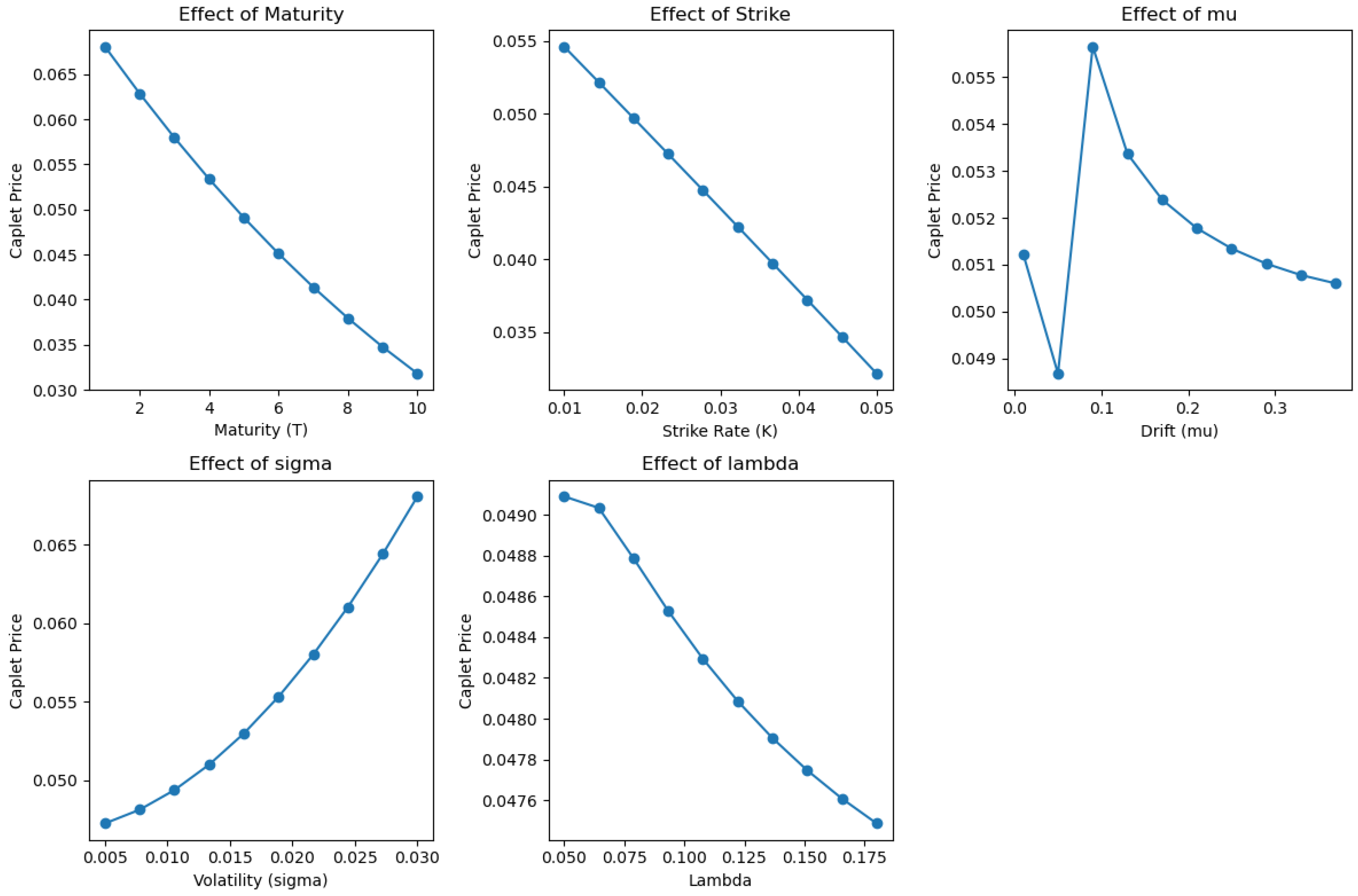
Figure 4.
Swaption price sensitivity computed via Monte Carlo simulation. Note the convex dependence on volatility and mean reversion.
Figure 4.
Swaption price sensitivity computed via Monte Carlo simulation. Note the convex dependence on volatility and mean reversion.
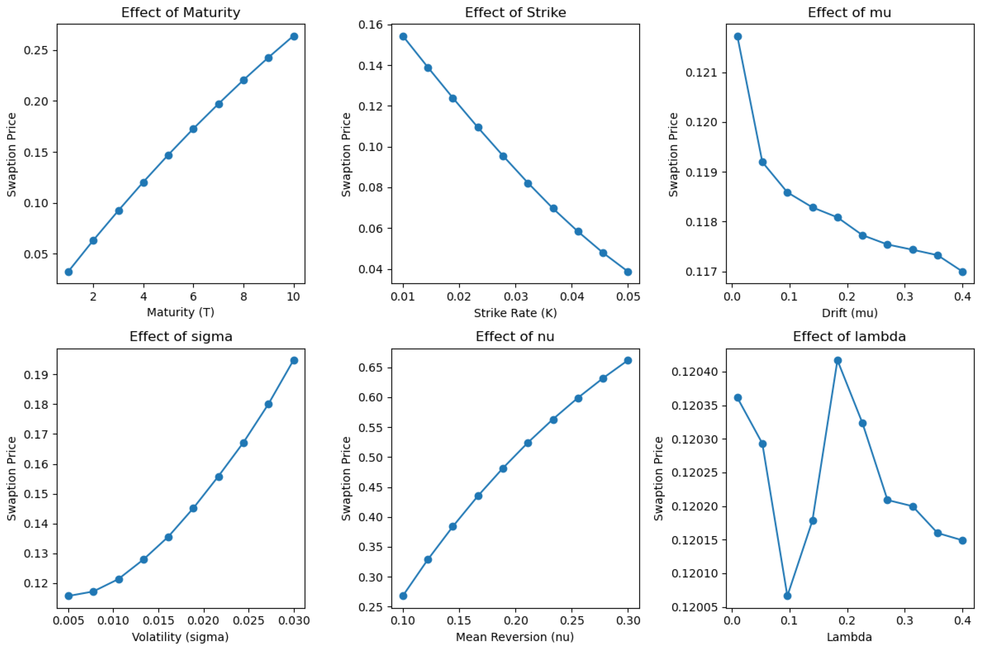
Figure 6.
Observed (dots) and model-implied (dashed lines) caplet prices for each month.
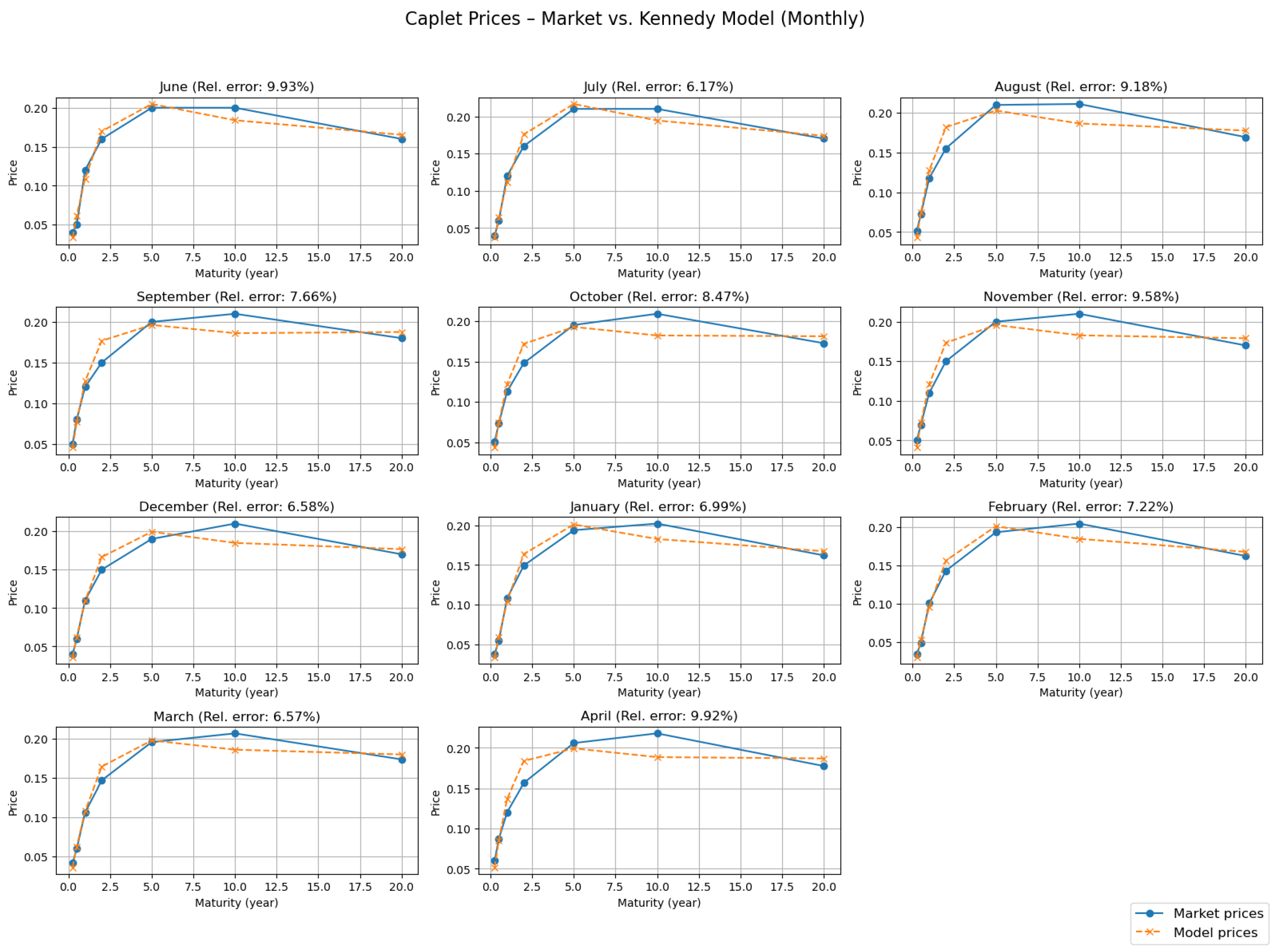
Figure 7.
Time series of the calibrated Kennedy model parameters , , and .
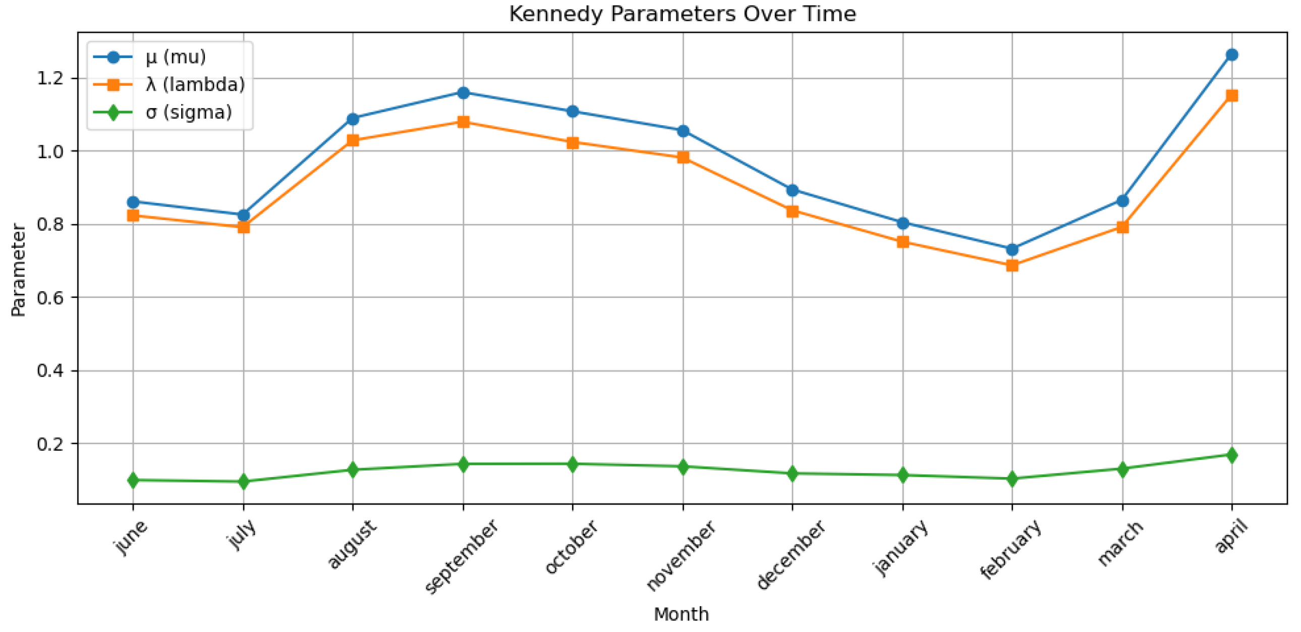
Figure 8.
Caplet prices by month: observed market prices (dots), model-implied prices (dashed lines), and forecasted prices using the previous month’s parameters (dotted green lines).
Figure 8.
Caplet prices by month: observed market prices (dots), model-implied prices (dashed lines), and forecasted prices using the previous month’s parameters (dotted green lines).
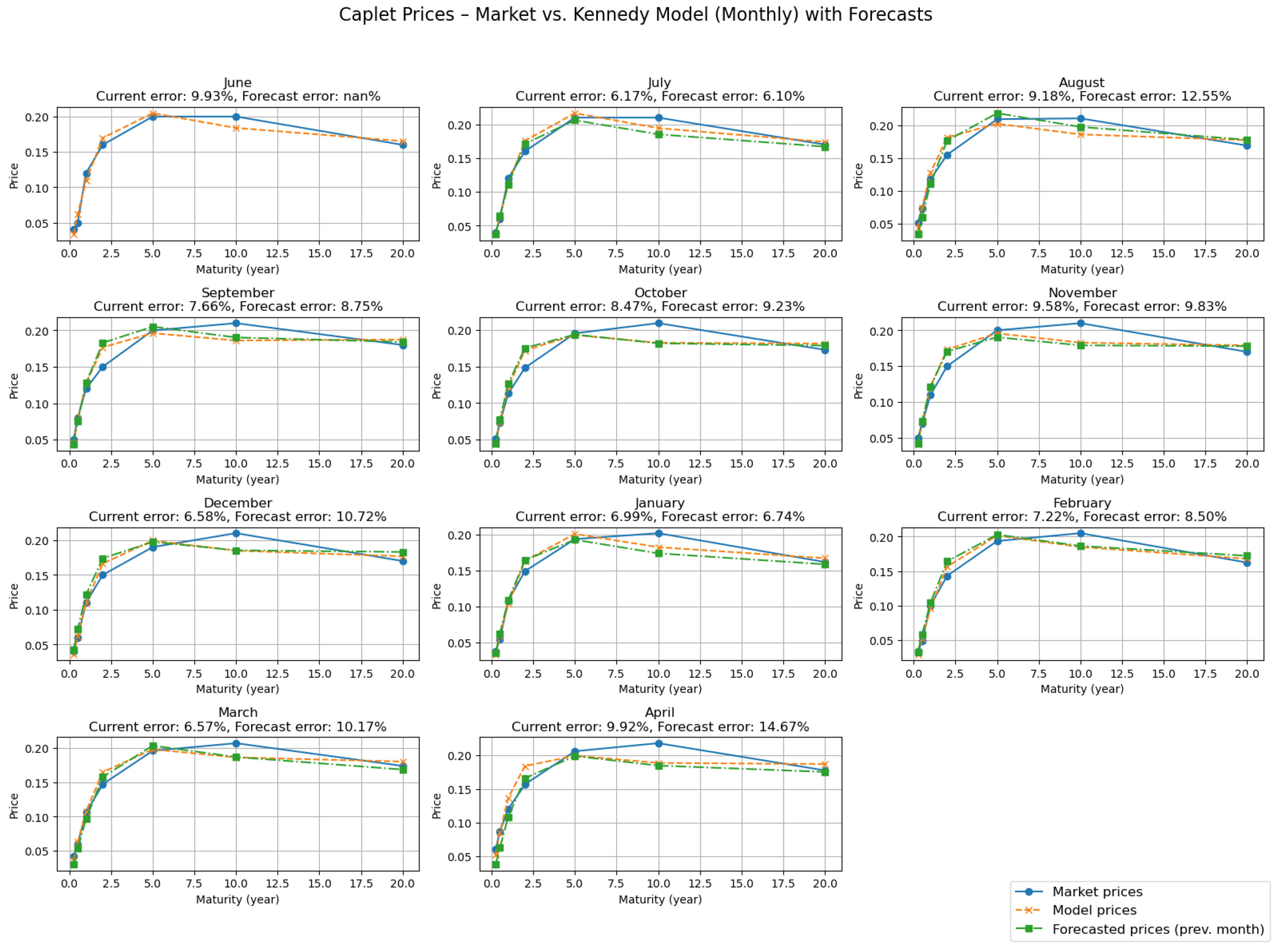
Figure 9.
Comparison of monthly average relative errors: in-sample calibration (orange) vs. one-step-ahead forecast (green).
Figure 9.
Comparison of monthly average relative errors: in-sample calibration (orange) vs. one-step-ahead forecast (green).
Disclaimer/Publisher’s Note: The statements, opinions and data contained in all publications are solely those of the individual author(s) and contributor(s) and not of MDPI and/or the editor(s). MDPI and/or the editor(s) disclaim responsibility for any injury to people or property resulting from any ideas, methods, instructions or products referred to in the content. |
© 2025 by the authors. Licensee MDPI, Basel, Switzerland. This article is an open access article distributed under the terms and conditions of the Creative Commons Attribution (CC BY) license (http://creativecommons.org/licenses/by/4.0/).
Copyright: This open access article is published under a Creative Commons CC BY 4.0 license, which permit the free download, distribution, and reuse, provided that the author and preprint are cited in any reuse.


