
Submitted:
03 November 2025
Posted:
03 November 2025
You are already at the latest version
Abstract
We propose a distribution–aware framework for unsupervised outlier detection that transforms multivariate data into one–dimensional neighborhood statistics and identifies anomalies through fitted parametric distributions. Supported by the CDF Superiority Theorem, validated through Monte Carlo simulations, the method connects distributional modeling with ROC–AUC consistency and produces interpretable, probabilistically calibrated scores. Across 23 real–world datasets, the proposed parametric models demonstrate competitive or superior detection accuracy with strong stability and minimal tuning compared with baseline non–parametric approaches. The framework is computationally lightweight and robust across diverse domains, offering clear probabilistic interpretability and substantially lower computational cost than conventional non–parametric detectors. These findings establish a principled and scalable approach to outlier detection, showing that statistical modeling of neighborhood distances can achieve high accuracy, transparency, and efficiency within a unified parametric framework.
Keywords:
outlier detection
; high-dimensional data
; parametric modeling
; kNN distance
; Manhattan distance
; distance transformation
; CDF-based scoring
; ROC–AUC
1. Introduction
Outlier detection is driven by several key objectives: preserving statistical validity by preventing extreme values from skewing summary statistics and invalidating inference [1], ensuring model robustness since many estimators are sensitive to anomalies [2], enhancing data quality through the flagging of measurement or entry errors [3], uncovering novel insights from rare events such as fraud or equipment failures [4], and supporting timely decision making in critical domains such as finance, cybersecurity, and healthcare [2]. Outlier detection is essential because extreme observations can bias our estimates, corrupt the fitting of the model, and obscure genuine rare events [1,2]. While many classical techniques work well in low-dimensional settings, they break down once the data’s dimensionality grows. In high-dimensional spaces, the “curse of dimensionality” causes distances to concentrate and data to become sparse, irrelevant features mask true anomalies, and the search space explodes—making outlier detection both harder and yet more critical in areas like fraud detection, genomics, and network security [5,6].
High-dimensional outlier detection is challenging due to the “curse of dimensionality”: as the number of features increases, the data become sparse and distance measures lose contrast, making proximity- and density-based methods unreliable [5,6]. Moreover, irrelevant or noisy dimensions can mask true anomalies and exponentially increase computational cost [2,6]. However, effective detection remains critical in domains such as fraud detection [7], network intrusion analysis, genetics , image processing, and sensor networks, where rare outliers may signal security breaches, medical anomalies, or equipment failures.
To address these challenges, we propose a novel parametric outlier detection framework that leverages a uni-dimensional distance transformation to capture each point’s “degree of outlier-ness” while remaining computationally efficient irrespective of the ambient dimension. By representing the dataset with a single distance vector, our method avoids the exponential cost of high-dimensional sorting and preserves interpretability through a small set of distributional parameters. We fit a flexible parametric model—choosing among positively skewed or log-transformed normal families—to the transformed distances, which allows us to derive closed-form expressions for thresholding and to prove that, under mild assumptions on the underlying distribution, our estimator controls false alarm rates and maximizes statistical power. Empirical evaluations on multiple benchmark datasets demonstrate that our approach consistently outperforms state-of-the-art non-parametric methods in mean ROC–AUC, validating both its practical efficiency and its provable performance guarantees.
The proposed and state-of-the-art algorithms have been benchmarked using the popular ROC-AUC framework. To ensure consistency, the same evaluation protocol was applied to our proposed algorithms. The AUC is calculated as the integral of the True Positive Rate (TPR) from 0 to 1 with respect to the False Positive Rate (FPR), as shown in Equation (1):
To place this work in context, we first review some of the most prominent existing approaches in both non-parametric and parametric outlier detection methods.
2. Literature Review
Outlier detection has long been studied from both data–driven and model–based perspectives. A substantial body of non-parametric research leverages the geometry or local density of data. For example, the k-nearest neighbor (KNN) distance method identifies outliers as points whose average distance to their k nearest neighbors is unusually large. [8,9], while density–based methods such as LOF, COF, and ABOD compare each point’s local density to that of its neighborhood to identify sparse regions [10,11,12]. These techniques make few assumptions about the underlying distribution and adapt well to complex, nonlinear structure. However, their performance tends to degrade in high dimensions—distances concentrate, noise dimensions mask true anomalies, and the computational cost of neighborhood or density estimation grows prohibitively with feature count [13,14]. Comprehensive evaluations and benchmark suites further document these effects and provide standardized comparisons across algorithms [14].
A second strand of non–parametric work refines these ideas. For example, Rehman and Belhaouari [13] propose KNN–based dimensionality reduction (D-KNN) to collapse multivariate data into a one–dimensional distance space, then apply box–plot adjustments and joint probability estimation to better separate outliers. Classical exploratory tools still inform practice: Tukey’s 1.5×IQR rule remains a widely used heuristic for flagging extreme points [15]. Distance choice is also critical in high-dimensional settings: Aggarwal et al. [9] showed that the (Manhattan) distance preserves greater contrast than the (Euclidean) distance as dimensionality increases, thereby enhancing the effectiveness of nearest-neighbor–based detection methods.
Parametric approaches offer an alternative by imposing distributional structure, yielding interpretable tests and often lower computational burden. Early methods include Grubbs’ test and standardized residuals under normality [16], with extensions such as Rosner’s generalized ESD procedure and the Davies–Gather and Hawkins tests to detect multiple outliers when the number of anomalies is known a priori [3,17,18]. More recent work develops robust tests for broader location–scale and shape–scale families (e.g., exponential, Weibull, logistic) that avoid pre–specifying the number of outliers [19]. In time–series and regression contexts, parametric residual–based techniques using exponential or gamma error models are used to identify anomalous behavior and heavy–tailed departures [20,21].
2.1. State of the Art
Modern anomaly detection systems span a broad spectrum, ranging from classical locality and density-based algorithms to modern representation-learning approaches. On the classical side, widely used methods include KNN [22], LOF [23], SimplifiedLOF [24], LoOP [25], LDOF [26], ODIN [27], FastABOD [28], KDEOS [29], LDF [30], INFLO [31], and COF [32]. These methods remain widely adopted, computationally efficient, and assumption-light, thereby constituting strong state-of-the-art baselines for tabular anomaly detection. Beyond these, the Isolation Forest (iForest) isolates anomalies via random partitioning [33], while the one-class SVM provides a large-margin boundary in high-dimensional feature spaces [34]. For learned representations, autoencoders, Deep SVDD, and probabilistic hybrids such as DAGMM often achieve leading results on image and complex tabular benchmarks [35,36]. Lightweight projection-based schemes such as HBOS and LODA deliver excellent speed–accuracy trade-offs [37,38], while the copula-based COPOD provides fully unsupervised, distribution-free scoring with competitive accuracy [39]. Together, these tools define the contemporary landscape of anomaly detection—from interpretable, efficient heuristics to flexible deep models.
2.2. Our Contribution in Context
Although grounded in different philosophies, both research lines ultimately aim to balance sensitivity to genuine anomalies with robustness against noise. Non-parametric methods perform well when no clear distributional form is present, yet they often suffer from the curse of dimensionality. Parametric tests, by contrast, regain efficiency and offer finite-sample guarantees under correct model specification, but are vulnerable to misspecification. In this paper, we unify these paradigms by introducing a uni-dimensional distance transformation that maps any dataset—regardless of its original dimension—into a single distance vector, which is then modeled with a flexible parametric distribution. This hybrid approach preserves interpretability and scalability, enables closed-form inference, and delivers provable performance under mild assumptions.
Building on the gaps identified above, the paper proceeds as follows. We first formalize a CDF Superiority Theorem, establishing that a parametric CDF–based score achieves strictly higher ROC–AUC than the KNN distance under mild conditions. We further outline the proof that this parametric score also outperforms any other non-parametric method. We then validate this theoretical advantage through Monte Carlo experiments, demonstrating that the mean ROC–AUC across 500 simulation paths under the gamma distribution exceeds that of five established non-parametric methods: KNN, LOF, ABOD, COF, and CDF. We then introduce our practical framework: reduce high-dimensional data to a 1-D KNN (Manhattan) distance vector; fit either positively skewed families (e.g., gamma/Weibull) or—after a log transform—normal-like families (normal/t/skew-normal); and score observations by their fitted CDFs. Next, we benchmark our approach against several state-of-the-art nonparametric baselines using 23 publicly available datasets. These 23 datasets are separated into two distinct categories: the literature set and the semantic set. The literature set includes commonly used datasets in previous papers that may lack real-world labels and might be synthetic or have outliers defined from prior papers. The semantic set outlines outliers based on sematic or domain meaning, they are not arbitrary or synthetic but infer anomalies based real world deviations, i.e. errors in manufacturing.
We report performance in terms of ROC–AUC, together with goodness-of-fit () derived from QQ plots of fitting proposed probaility distriutions with 1-D KNN distance vector. We then examine the relationship between fit quality and detection accuracy, highlighting the conditions under which the parametric approach is most effective. Finally, we conclude with key implications and directions for future research.
3. Method and Theoretical Results
Suppose that we originally have a data set in a N-dimensional space. According to Rehman and Belhaouari [13], this dataset can be effectively transformed into a one-dimensional distance space by employing a suitable metric such as Manhattan distance or Euclidean distance. Specifically, for each observation in the original N-dimensional space, the distance to its nearest neighbor is computed. This process generates a new dataset consisting solely of these distances, denoted as . Formally, this transformation can be represented as:
Each represents the distance from a point to its nearest neighbor, corresponding to the maximum distance within its k-neighbor set. We adopt the Manhattan distance here, calculated as the absolute sum of the differences between Cartesian coordinates. The rationale for using Manhattan distance is grounded in the work of Aggarwal et al. [9] on distance metrics in high-dimensional spaces. Compared to Euclidean distance, Manhattan distance lowers the density peak while spreading values more broadly, resulting in a longer-tailed distribution. This characteristic reduces the likelihood of misclassifying inliers as outliers. In high-dimensional settings, this effect becomes even more pronounced, as certain data points—referred to as “hubs"—tend to emerge as the nearest neighbors for a disproportionately large number of other points. Such uneven distribution contributes to the skewness observed in the nearest neighbor distances [40].
Building on this foundation, it has been observed that as dimensionality increases, (Euclidean) distances tend to concentrate due to an exaggeration effect that distorts the relative positioning of outliers. In contrast, (Manhattan) distance is more robust to this effect and better captures the skewness and variability inherent in the data [9]. This distinction is especially significant under the curse of dimensionality, where, as the number of dimensions grows, KNN distances become increasingly equidistant. This equidistance causes distances to shrink and creates a positvely-skewed distribution [9]. As shown in Equation (3)
and discussed in Aggarwal et al. [9], substituting with introduces greater variability, which slows down the convergence of distances toward uniformity, therefore mitigating the equidistant effect.
After reducing the multidimensional data to a one-dimensional array using KNN with Manhattan distance, we fit the resulting distribution to a family of positively skewed distributions.
3.1. Positively-Skewed Distributions
Parametric methods offer several advantages over non-parametric approaches, including clearer interpretation, greater accuracy, and easier calculations. Parametric statistics relies on the underlying assumption that the data are from a specific distribution. The set satisfies these assumptions by being nonnegative, positively skewed, and adheres to the shape and scale parameters of a positively skewed distribution. Since most of the data will be clustered together, a sharp increase and gradual decrease in density will plague the data. Skewness seems to be related to the phenomenon of distance concentration, defined as a ratio of some spread and magnitude of distances [40]. The resultant data exhibit positive skewness, with a long right tail representing values distant from both the mean and median. To model this behavior, we fit a family of positively skewed distributions to the one-dimensional data.
From Positioning to Theory
The discussion above motivates a hybrid scoring rule: reduce high–dimensional data to a one–dimensional summary and then apply a parametric score that aligns with the inlier distribution. We now provide a theoretical justification for this choice by comparing a distribution–aware score to a purely geometric one. Specifically, we consider two outlier scores for a point x: (i) the CDF score of the inlier distribution, which is a monotone transform of the optimal likelihood ratio, and (ii) the KNN distance score , a standard nonparametric baseline. Using ROC–AUC as our comparison criterion,
We show that, under mild regularity conditions (continuous and strictly positive densities), the CDF-based score strictly dominates the KNN distance: it yields fewer pairwise misorderings between outliers and inliers, and therefore achieves a larger AUC. This result formalizes why a univariate, distribution-aligned score can outperform distance-based heuristics, particularly in regimes where distances lose contrast.
To rigorously substantiate this intuition, we now present a formal result that characterizes when and why CDF-based scoring functions outperform KNN distances in ranking performance. We state the result next.
3.2. Behavior of Continuous Density Function Versus Non-Parametric for ROC-AUC Scores
This section introduces the CDF Superiority Theorem, illustrates it with two numerical examples, and validates it through simulation results.
3.2.1. The CDF Superiority Theorem
Statement of the Theorem.Let and be independent draws from two continuous densities on , each strictly positive everywhere. We compare two outlier-scoring rules:
- CDF score:
- KNN distance score:
We use the standard ROC–AUC definition
Then
Proof of the Theorem. Let and be independent draws from continuous, strictly positive densities on . For any scoring rule T, define its mis–ordering set
Then
(1) CDF Score.
For the CDF score , F is strictly increasing, hence . Setting
Equation (4) yields .
(2) KNN Distance Score.
Let be the distance from x to its kth nearest neighbor within an i.i.d. sample . Its mis–ordering set is and
Split
We claim . Fix . For let (). Each has a continuous, strictly positive density on ; the kth nearest–neighbor distance is the kth order statistic . The vector has a positive joint density on , and the smooth, one-to-one a.e. mapping to implies that the pair has a continuous joint density h that is positive on . Therefore
Since is strictly positive for all , integrating this strictly positive probability over the set yields .
(3) Conclusion.
We have
Hence, the CDF score attains a strictly larger ROC-AUC than the KNN distance score.
3.2.2. Extension to Other Nonparametric Methods
The same argument applies to any other non-parametric outlier score. Here is an outline of the proof.
-
ROC–AUC cares only about pairwise ordering..
-
The CDF score is strictly monotonic in x.increases strictly, so it never mis-orders any .
-
Any non-parametric method must mis-order a positive-measure set of pairs.Estimated from finite data (LOF, isolation forest, etc.), it cannot perfectly reproduce the CDF ordering, so there exist with with positive probability.
-
Strict AUC gap follows.Let and the mis-order probability of the non-parametric score. Thenso .
Remark. Because any non-parametric rule must mis-order some inlier–outlier pairs with positive probability, its ROC–AUC is strictly lower than the ideal CDF rule’s.
3.2.3. Significance of the CDF Superiority Theorem
Under mild regularity conditions, assuming continuous and strictly positive densities, the CDF Superiority Theorem establishes a theoretical guarantee for distribution-aware scoring in anomaly detection. Ranking observations by the inlier CDF —for example, using the tail score —achieves a strictly higher ROC–AUC than ranking by KNN distances. The result follows from the probability integral transform: if , then is uniformly distributed on . Since the ROC curve is invariant under strictly monotonic transformations of a score [41,42], any monotone function of yields the same ROC performance. In practice, this motivates methods that map data to a one-dimensional statistic aligned with the inlier distribution and then apply a distribution-matched score. When the model is reasonably well specified, such CDF-based scoring provides a consistent advantage in ranking performance.
3.2.4. Theoretical Support for Parametric Tests
The CDF Superiority Theorem in this paper shows that, under mild regularity and a correctly (or well) specified inlier model F, ranking observations by the inlier CDF—equivalently, by the tail score —achieves a strictly higher ROC–AUC than geometric KNN distance scores. This result provides a principled foundation for parametric outlier procedures that base decisions on model-derived tail probabilities or residuals. In particular, it theoretically supports the multiple-outlier tests of Bagdonavičius and Petkevičius [43], which assume a parametric family for the inlier distribution and identify extreme observations via distribution-aware statistics on orderings of the sample. When the assumed family approximates the true inlier law, our theorem predicts that CDF-based rankings (and the associated p-value thresholds) are optimal in the ranking sense, explaining the empirical effectiveness of model-based multi-outlier tests and motivating their use over purely distance-based heuristics.
3.3. Worked Examples
3.3.1. KNN Distance Example
Dataset (1D): Inliers ; Outliers . Choose . Compute 2-NN distances among :
CDF ordering demands . Pick : since , , yet
so the KNN score mis-orders that inlier–outlier pair.
3.3.2. LOF Example ()
Dataset: with 0,1 inliers and 4 outlier.
Reachability distances:
Local reachability densities:
LOF scores:
Pick : although , we have so LOF mis-orders that inlier–outlier pair.
Remark
KNN distance can assign identical scores to even though . LOF can assign the same score to inlier and outlier, violating the true CDF ranking.
Thus, any nonparametric method like KNN or LOF must strictly underperform the CDF-based score in ROC–AUC: it mis-orders some positive-probability inlier–outlier pairs.
In practice we don’t compute the integral
directly, but rather approximate it by the fraction of mis-ordered pairs in the finite data set. Concretely, if we have N inliers and M outliers, we form all pairs and compute
Even though the true probability , it’s quite possible—especially if N and M are small, or if the score ties a lot—that you observe zero mis-ordered pairs in this sample, i.e. . That in turn makes the empirical AUC hit its maximum of 1.0.
The theorem guarantees that in the population limit, that is, as the number of data points approaches infinity. In finite samples, however, random fluctuations may cause the empirical estimate to be zero simply because, by chance, no misordered pairs are observed within the Monte Carlo sample.
As N and M grow larger, or as the experiment is repeated, the chance that becomes smaller, roughly at an exponential rate in . However, this probability does not disappear entirely until the sample size tends to infinity.
In conclusion, the sample size must be sufficiently large to mitigate random misorderings arising from sampling variability. Since the CDF is estimated probabilistically, finite-sample fluctuations can cause certain points to be overestimated and thus mistakenly classified as outliers. In practice, a larger sample reduces this Monte Carlo noise and yields a ranking that better reflects the true ordering implied by the underlying distributions.
3.4. Monte Carlo Simulation of Gamma CDF Versus Non-Parametric ROC-AUC Scores
To empirically validate the proof that the CDF-based ranking outperforms non-parametric methods, a Monte Carlo simulation was conducted in Python. It is built upon the injection of outliers into a random gamma distribution before evaluating each method by running 500 simulations. Shape and scale of the gamma distribution was obtained by fitting 200 training point for each simulation run and the method of estimation was maximum likelihood estimation (MLE). These parameters acted as the base for the cumulative density function in evaluating the 400 randomly generated (predetermined shape and scale parameters) gamma inlier and outlier test points. Each simulation tested KNN, LOF, ABOD, COF, and gamma CDF to determine the best ROC-AUC score. Table 1 presents a summary of the overall simulation results. Table 2 summarizes the shape and scale parameters used in the training and testing sets. Gamma CDF was the best performing outlier detector in the Monte Carlo simulation as expected from experimental validation of the CDF Superiority theorem proof. Python code Listing in Appendix A contains the detailed python code for implementation.

Table 1.
ROC-AUC Scores as per each method for Monte Carlo simulation.
| mean | std | min | 25% | 50% | 75% | max | |
|---|---|---|---|---|---|---|---|
| KNN | 84.8% | 2.1% | 78.4% | 83.4% | 84.9% | 86.3% | 90.5% |
| LOF | 63.0% | 5.9% | 43.8% | 58.8% | 62.8% | 67.3% | 78.1% |
| ABOD | 80.7% | 2.4% | 73.3% | 79.1% | 80.8% | 82.2% | 86.3% |
| COF | 50.6% | 2.5% | 43.3% | 48.9% | 50.5% | 52.2% | 57.7% |
| Gamma CDF | 89.1% | 1.5% | 84.8% | 88.1% | 89.1% | 90.2% | 93.4% |
Table 2.
Shape and scale parameters for training and testing sets.
| Train | Test Inlier | Test Outlier | |
|---|---|---|---|
| Shape | 2.0 | 2.0 | 5.0 |
| Scale | 2.0 | 2.0 | 2.0 |
An important takeaway from the CDF proof and Monte Carlo simulation is that the cumulative distribution function outperforms non-parametric methods only when the goodness of fit is exceptionally high and the sample size is sufficiently large.
4. Our Parametric Outlier-Detection Framework
We propose a two–stage pipeline: (i) reduce the data to a one–dimensional distance statistic that preserves the degree of “outlier-ness’’ even in high dimension, and (ii) fit a parametric family to that statistic and score points by calibrated tail probabilities. This design keeps computation light, retains interpretability, and—by working with a 1-D summary—avoids the distance–concentration pitfalls of high-d spaces [5].
4.1. Dimensionality Reduction via KNN–Manhattan
For each observation , we compute the distance to its kth nearest neighbor under the 1 metric,
Using 1 (Manhattan) rather than 2 (Euclidean) helps retain spread and ranking contrast as n grows [9]; it also mitigates hubness, where a few points become nearest neighbors of many others and distort scores [40]. Empirically, the empirical distribution of is typically right-skewed, which motivates the parametric fits below.
4.2. Fitting Positively Skewed Distributions
Let denote the dataset of one-dimensional distances. We fit using a family of positively skewed distributions via the maximum likelihood estimation (MLE) method. This family includes Normal-like distributions such as the log-normal, log-Student-t, log-Laplace, log-logistic, and log-skew-normal, as well as other positively skewed distributions including the exponential, chi-squared (), gamma, Weibull-minimum, inverse Gaussian, Rayleigh, Wald, Pareto, Nakagami, logistic, power-law, and skew-normal distributions. Denoting a generic density by with parameter , we maximize
For example, the gamma PDF is , and the Weibull PDF is . After fitting, we score a point by its right-tail probability under the fitted CDF ,
which is a calibrated, distribution-aligned p-value. Rankings are invariant to monotone transforms, so we can equivalently use .
Log–Transform and Normal-like Fits
We follow the ladder-of-powers guideline that lower-power transforms (log, square-root) reduce positive skew [15]. When the distance sample is strictly positive and right-skewed, we set and fit location–scale families on : normal , Student- for heavier tails, and logistic; to absorb any residual asymmetry we also include the skew-normal with shape parameter [44]. Outlier scores are computed on the original scale via the fitted CDF of ,
which is equivalent to using right-tail z-scores for normal-like fits. This “log-transform branch” complements the positive-skew families and improves robustness whenever the log transform approximately symmetrizes the distance distribution.
4.3. Baseline Non-Parametric Methods
We implement a set of standard baselines widely used in the outlier detection literature, including KNN, LOF, SimplifiedLOF, LoOP, LDOF, ODIN, FastABOD, KDEOS, LDF, INFLO, and COF. For these 11 baseline methods, we report results under both 1 and 2 metrics. All methods score by decreasing density (or increasing distance) and are evaluated by ROC–AUC.
4.4. Datasets
As mentioned in the last subsection of Section 2 (Literature Review), we evaluate both the baseline methods and our proposed approaches on 23 datasets, including 11 literature datasets and 12 semantic datasets. A descriptive summary of the two dataset types is provided in Table 3. All datasets were obtained from Campos et al. [14]. The semantic datasets, in particular, have been modified to better reflect real-world occurrences of outliers. Each dataset varies on the number of outliers included, ranging from as low as to as high as . Campos et al. [14] provided results for multiple levels of outlier percentages for most datasets, therefore, we chose to focus on the highest outlier levels for they contain all observations instead of being a subset.
Table 3.
Details of datasets used for comparison.
| Name | Type | Instances | Outliers | Attributes |
|---|---|---|---|---|
| ALOI | Literature | 50,000 | 1508 | 27 |
| Glass | Literature | 214 | 9 | 7 |
| Ionosphere | Literature | 351 | 126 | 32 |
| KDDCup99 | Literature | 60,632 | 246 | 38+3 |
| Lymphography | Literature | 148 | 6 | 3+16 |
| PenDigits | Literature | 9,868 | 20 | 16 |
| Shuttle | Literature | 1,013 | 13 | 9 |
| Waveform | Literature | 3,443 | 100 | 21 |
| WBC | Literature | 454 | 10 | 9 |
| WDBC | Literature | 367 | 10 | 30 |
| WPBC | Literature | 198 | 47 | 33 |
| Annthyroid | Semantic | 7,200 | 534 | 21 |
| Arrhythmia | Semantic | 450 | 206 | 259 |
| Cardiotocography | Semantic | 2,126 | 471 | 21 |
| HeartDisease | Semantic | 270 | 120 | 13 |
| Hepatitis | Semantic | 80 | 13 | 19 |
| InternetAds | Semantic | 3,264 | 454 | 1,555 |
| PageBlocks | Semantic | 5,473 | 560 | 10 |
| Parkinson | Semantic | 195 | 147 | 22 |
| Pima | Semantic | 768 | 268 | 8 |
| SpamBase | Semantic | 4,601 | 1,813 | 57 |
| Stamps | Semantic | 340 | 31 | 9 |
| Wilt | Semantic | 4,839 | 261 | 5 |
5. Empirical Results
Before examining the outlier-detection performance summarized in Tables 4 and 5, it is instructive to first assess how well the proposed parametric families capture the underlying data distributions. To this end, we analyze the goodness-of-fit results based on the values from QQ plots, as summarized in Tables A1–A4.
Table 4.
Literature datasets ROC-AUC averages.
| Average | ||
|---|---|---|
| ROC AUC | ||
| Log Transform | ||
| norm | 87.34% | |
| t | 87.56% | |
| laplace | 87.48% | |
| logistic | 87.35% | |
| skewnorm | 87.55% | |
| No Transform | ||
| expon | 87.10% | |
| chi2 | 87.52% | |
| gamma | 87.29% | |
| weibull_min | 87.40% | |
| invgauss | 87.56% | |
| rayleigh | 87.13% | |
| wald | 87.37% | |
| pareto | 87.47% | |
| nakagami | 87.45% | |
| logistic | 86.52% | |
| powerlaw | 87.35% | |
| skewnorm | 87.25% | |
| Baseline Manhattan | ||
| KNN | 87.53% | |
| LOF | 84.75% | |
| SimplifiedLOF | 86.76% | |
| LoOP % | 83.41% | |
| LDOF | 79.66% | |
| ODIN | 87.62% | |
| FastABOD | 64.55% | |
| KDEOS | 75.37% | |
| LDF | 86.76% | |
| INFLO | 83.07% | |
| COF | 81.51% | |
| Baseline Euclidean | ||
| KNN | 87.66% | |
| LOF | 85.61% | |
| SimplifiedLOF | 83.44% | |
| LoOP | 83.27% | |
| LDOF | 83.02% | |
| ODIN | 82.64% | |
| FastABOD | 87.65% | |
| KDEOS | 73.11% | |
| LDF | 86.29% | |
| INFLO | 83.16% | |
| COF | 84.02% |
Table 5.
Semantic datasets ROC-AUC averages.
| Average | ||
|---|---|---|
| ROC AUC | ||
| Log Tranform | ||
| norm | 72.34% | |
| t | 72.33% | |
| laplace | 72.35% | |
| logistic | 72.33% | |
| skewnorm | 72.38% | |
| No Tranform | ||
| expon | 71.86% | |
| chi2 | 72.26% | |
| gamma | 72.30% | |
| weibull_min | 72.18% | |
| invgauss | 72.38% | |
| rayleigh | 72.29% | |
| wald | 72.32% | |
| pareto | 72.32% | |
| nakagami | 72.32% | |
| logistic | 72.23% | |
| powerlaw | 72.27% | |
| skewnorm | 72.30% | |
| Baseline Manhattan | ||
| KNN | 72.33% | |
| LOF | 69.16% | |
| SimplifiedLOF | 71.34% | |
| LoOP | 65.76% | |
| LDOF | 65.37% | |
| ODIN | 72.37% | |
| FastABOD | 62.35% | |
| KDEOS | 62.06% | |
| LDF | 71.34% | |
| INFLO | 65.64% | |
| COF | 64.34% | |
| Baseline Euclidean | ||
| KNN | 70.93% | |
| LOF | 69.31% | |
| SimplifiedLOF | 66.72% | |
| LoOP | 65.92% | |
| LDOF | 65.85% | |
| ODIN | 65.35% | |
| FastABOD | 67.00% | |
| KDEOS | 62.10% | |
| LDF | 70.83% | |
| INFLO | 64.59% | |
| COF | 68.54% |
5.1. Analysis of Goodness-of-Fit Across Literature and Semantic Datasets
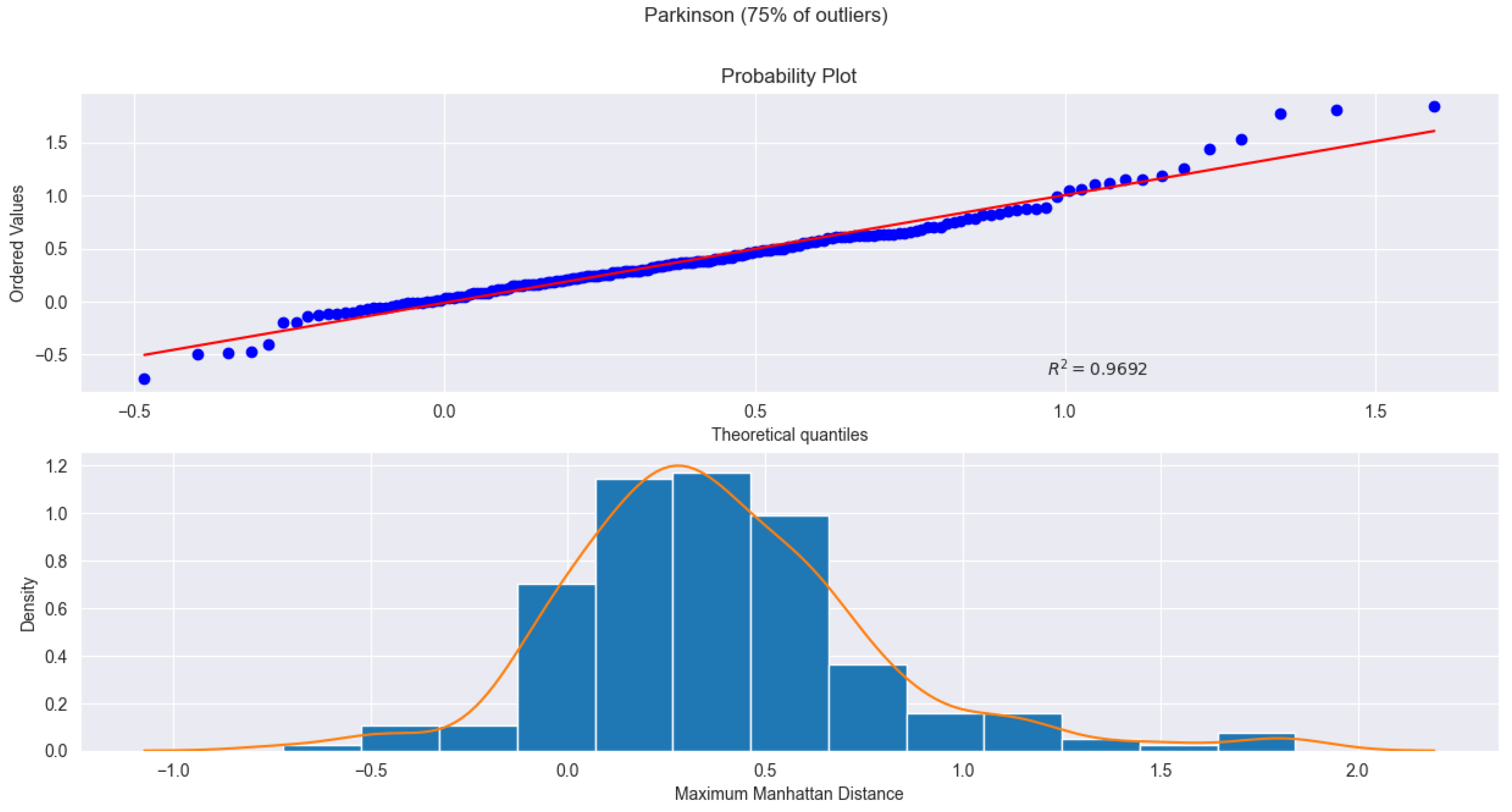
Table A1–A4 summarize the values across both log-transformed and untransformed settings. Log-transformed models consistently yield higher values (94–99%), confirming their stability and closer alignment with theoretical quantiles. For the literature datasets, the log-transformed normal, Student-t, and skew-normal distributions perform best; for the semantic datasets, the skew-normal and Student-t distributions remain the strongest. Two representative examples of fitted distributions are shown in Figure 1 and Figure 2: the Arrhythmia dataset (Fig. Figure 1) achieves an under a gamma distribution, while the Parkinson dataset (Fig. Figure 2) attains an under a skew-normal distribution after log transformation. Both figures show strong agreement between theoretical and empirical quantiles, reinforcing that log transformation enhances fit quality and that the proposed parametric framework remains robust across diverse data types while supporting high detection accuracy.
5.2. Real Data Analysis Results
After evaluating 17 parametric distributions—12 positively skewed and 5 approximately symmetric—across 23 datasets, the proposed parametric fits on the one-dimensional distance function (optionally after a log transform) achieve KNN-level or higher accuracy while consistently outperforming other baseline detectors. In the literature datasets, the log-transformed Student-t and the inverse Gaussian (without log transformation) distributions both achieve the highest average ROC–AUC of 87.56%, matching or slightly exceeding KNN– (87.53–87.66%) and clearly outperforming LOF, COF, KDEOS, and FastABOD, which frequently fall below 85%. Per-dataset analyses (Tables A5–A8) show stable wins or ties for the parametric models, with notable advantages in moderately skewed datasets such as PIMA (73.7% vs. KNN–L1 67%) and strong robustness in highly skewed ones like KDDCup99 and WDBC, where fitted distributions maintain near-perfect detection accuracy (>96%). On the semantic datasets (Tables A9–A12), the best-performing parametric distributions—the skew-normal under log transformation and the inverse Gaussian without log transformation—achieve an average ROC–AUC of 72.38%, essentially matching and slightly exceeding KNN– (72.33%), while outperforming LOF (≈69%), KDEOS (≈65%), COF (≈60%), and ABOD (≈63%). Certain baseline methods, including LDOF and FastABOD, were computationally infeasible for several large datasets (as indicated in Tables A5–A12), underscoring the practical advantage of the lightweight parametric approach. These results confirm that a small and interpretable family of fitted distributions, once paired with a simple neighborhood scale k, provides competitive accuracy with far less parameter tuning.
When comparing Tables 4 and 5 together, both domains show a similar drop in absolute performance, yet the parametric methods remain remarkably uniform across transformations and dataset types. Their average ROC–AUC stays within a narrow band (≈87% → 72%), indicating strong distributional adaptability and low sensitivity to distance-metric choice. In contrast, baseline methods exhibit wider fluctuations and sharper degradation. Several factors explain the superiority of the parametric framework: (1) performance consistency, as it maintains nearly identical rankings across datasets, highlighting reliable generalization; (2) statistical interpretability, since each fitted distribution (e.g., t, inverse-Gaussian, skew-normal) conveys explicit probabilistic semantics—tail behavior, variance, and skewness—that yield explainable anomaly thresholds; (3) computational efficiency, because once parameters are estimated, new-sample scoring becomes lightweight compared with K-neighbor searches; and (4) practical robustness, since these models attain equal or higher ROC–AUC than KNN or ODIN without heavy hyperparameter tuning. When performance levels are close, interpretability becomes decisive—the parametric models provide transparent probabilistic reasoning while achieving comparable or better accuracy. Overall, across both literature and semantic datasets, these results establish the proposed parametric approach as a simple, interpretable, and high-performing alternative to traditional distance-based outlier detectors.
6. Conclusion
We proposed a distribution–aware framework for unsupervised outlier detection that reduces multivariate data to one–dimensional neighborhood statistics and identifies anomalies through fitted parametric distributions. Supported by the CDF Superiority Theorem, this approach connects distributional modeling with ROC–AUC consistency and produces interpretable, probabilistically calibrated scores.
Across 23 datasets, the proposed parametric families deliver competitive or superior detection accuracy with remarkable stability and minimal tuning. The framework remains computationally lightweight and robust even on semantically complex datasets, outperforming most traditional distance- and density-based baselines that often require costly hyperparameter optimization. For those baselines exhibiting comparable accuracy, our parametric models further offer clear probabilistic interpretability and substantially lower computational cost.
Overall, these results highlight a principled and interpretable pathway for outlier detection, showing that statistical modeling of neighborhood distances can achieve strong, reliable performance without reliance on heavy non-parametric machinery.
Author Contributions
Conceptualization, Jie Zhou; Formal Analysis, Jie Zhou, Weiqiang Dong, Emmanuel Tamakloe, and Karson Hodge; Methodology, Jie Zhou, Weiqiang Dong, Emmanuel Tamakloe, and Karson Hodge; Project Administration, Jie Zhou; Software, Jie Zhou and Karson Hodge; Supervision, Jie Zhou, Weiqiang Dong, and Emmanuel Tamakloe; Validation, Jie Zhou, Weiqiang Dong, Emmanuel Tamakloe, and Karson Hodge; Visualization, Jie Zhou and Karson Hodge; Writing—original draft, Jie Zhou and Karson Hodge; Writing—review & editing, Jie Zhou, Weiqiang Dong, Emmanuel Tamakloe, and Karson Hodge. All authors have read and agreed to the published version of the manuscript.
Funding
This research received no external funding.
Institutional Review Board Statement
Not applicable.
Informed Consent Statement
Not applicablee.
Data Availability Statement
The data presented in this study are available in Outlier-Detection at https://github.com/hodge-py/Outlier-Detection. These data were derived from the following resource available in the public domain: https://www.dbs.ifi.lmu.de/research/outlier-evaluation/DAMI/.
Acknowledgments
During the preparation of this manuscript/study, the authors used ChatGPT for the purposes of editing statements and correcting grammatical errors. The authors have reviewed and edited the output and take full responsibility for the content of this publication.
Conflicts of Interest
The authors declare no conflicts of interest.
Abbreviations
The following abbreviations are used in this manuscript:
| KNN | k-Nearest Neighbors |
| LOF | Local Outlier Factor |
| COF | Connectivity-Based Outlier Factor |
| ABOD | Angle-Based Outlier Factor |
| KDE | Kernel Density Estimation |
| CDF | Cumulative Distribution Function |
| TPR | True Positive Rate |
| FPR | False Positive Rate |
| ROC | Receiver Operating Characteristic |
| AUC | Area Under Curve |
| ESD | Extreme Studentized Deviate |
| LoOP | Local Outlier Probabilities |
| LDOF | Local Distance-Based Outlier Factor |
| ODIN | Outlier Detection for Networks |
| KDEOS | Kernel Density Estimation Outlier Score |
| SVM | Support Vector Machine |
| SVDD | Support Vector Data Description |
| DAGMM | Deep Autoencoding Gaussian Mixture Model |
| HBOS | Histogram-Based Outlier Score |
| LODA | Lightweight On-line Detector of Anomalies |
| COPOD | Copula-Based Outlier Detection |
| INFLO | Influenced Outlierness |
Appendix A
The code and additional experimental results can be https://www.dbs.ifi.lmu.de/research/outlier-evaluation/DAMI/, https://github.com/hodge-py/Outlier-Detection.
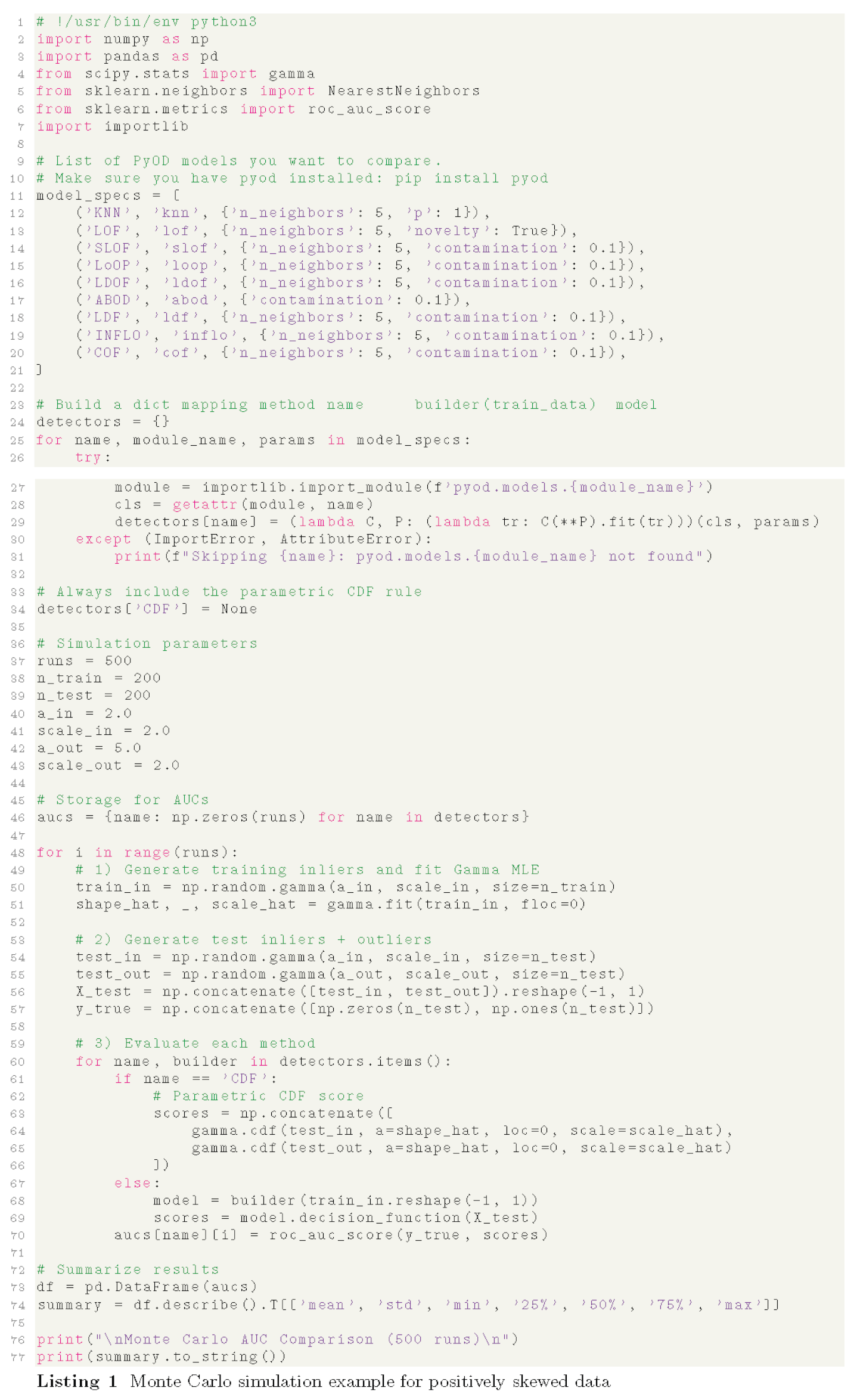
Table A1.
R2 for QQ Plots of Literature Datasets Part 1.
| ALOI | Glass | Ionosphere | KDDCup99 | Lymphogra | PenDigits | |
|---|---|---|---|---|---|---|
| Log Transform | ||||||
| norm | 98.81% | 93.36% | 98.36% | 90.25% | 92.44% | 97.88% |
| t | 98.86% | 91.38% | 98.36% | 88.38% | 96.71% | 97.66% |
| laplace | 95.66% | 90.36% | 91.60% | 88.98% | 90.75% | 93.12% |
| logistic | 98.42% | 92.25% | 96.12% | 90.08% | 94.47% | 96.69% |
| skewnorm | 99.71% | 98.72% | 98.30% | 95.60% | 97.85% | 99.86% |
| No Transform | ||||||
| expon | 89.28% | 93.64% | 97.14% | 76.67% | 96.17% | 99.36% |
| chi2 | 91.27% | 94.33% | 96.29% | 92.60% | 97.28% | 98.23% |
| gamma | 93.91% | 93.87% | 97.12% | 97.96% | 92.45% | 97.86% |
| weibull_min | 93.93% | 97.77% | 97.33% | 97.73% | 91.00% | 95.70% |
| invgauss | 99.13% | 95.99% | 93.88% | 99.18% | 94.22% | 96.39% |
| rayleigh | 69.15% | 75.77% | 90.79% | 52.58% | 79.50% | 93.74% |
| wald | 96.14% | 97.45% | 93.01% | 87.44% | 98.24% | 96.70% |
| pareto | 98.36% | 95.84% | 97.14% | 12.84% | 96.17% | 99.36% |
| nakagami | 82.07% | 84.00% | 97.45% | 76.86% | 87.64% | 94.71% |
| logistic | 61.71% | 71.96% | 80.61% | 46.46% | 79.73% | 87.25% |
| powerlaw | 73.65% | 86.12% | 96.79% | 63.82% | 76.63% | 87.89% |
| skewnorm | 75.15% | 81.96% | 95.23% | 58.90% | 88.14% | 96.78% |
Table A2.
R2 for QQ Plots of Literature Datasets Part 2.
| Shuttle | Waveform | WBC | WDBC | WPBC | Average | |
|---|---|---|---|---|---|---|
| Log Transform | ||||||
| norm | 99.10% | 99.14% | 87.33% | 90.96% | 92.60% | 94.57% |
| t | 99.29% | 99.12% | 83.70% | 85.60% | 89.97% | 93.55% |
| laplace | 97.02% | 95.62% | 82.65% | 87.74% | 89.02% | 91.14% |
| logistic | 99.09% | 98.39% | 83.39% | 91.31% | 90.83% | 93.73% |
| skewnorm | 99.25% | 99.96% | 93.28% | 97.87% | 98.95% | 98.12% |
| No Transform | ||||||
| expon | 73.73% | 91.97% | 91.40% | 95.57% | 99.17% | 91.28% |
| chi2 | 73.78% | 99.96% | 89.83% | 97.32% | 98.60% | 93.59% |
| gamma | 72.50% | 99.96% | 98.67% | 97.35% | 98.60% | 94.57% |
| weibull_min | 79.88% | 99.31% | 92.12% | 92.68% | 97.12% | 94.05% |
| invgauss | 73.43% | 99.97% | 89.77% | 97.18% | 99.11% | 94.39% |
| rayleigh | 62.81% | 99.71% | 64.23% | 79.35% | 92.52% | 78.19% |
| wald | 78.22% | 84.60% | 92.95% | 98.75% | 97.24% | 92.79% |
| pareto | 73.73% | 91.97% | 64.07% | 96.02% | 99.24% | 84.07% |
| nakagami | 64.77% | 99.66% | 88.02% | 86.87% | 94.98% | 87.00% |
| logistic | 59.31% | 97.13% | 58.20% | 72.55% | 83.44% | 72.58% |
| powerlaw | 56.20% | 93.50% | 72.40% | 76.42% | 89.13% | 79.32% |
| skewnorm | 65.54% | 99.90% | 71.21% | 85.54% | 95.16% | 83.04% |
Table A3.
R2 for QQ Plots of Semantic Datasets Part 1.
| Annthyroid | Arrhythmia | Cardiotocography | HeartDisease | Hepatitis | InternetAds | |
|---|---|---|---|---|---|---|
| Log Transform | ||||||
| norm | 97.32% | 92.53% | 98.33% | 98.37% | 96.42% | 97.22% |
| t | 99.12% | 91.14% | 98.23% | 98.37% | 96.42% | 97.22% |
| laplace | 98.76% | 90.17% | 94.26% | 93.94% | 89.60% | 93.41% |
| logistic | 98.97% | 92.01% | 97.23% | 97.15% | 93.92% | 96.18% |
| skewnorm | 97.48% | 99.49% | 99.44% | 99.31% | 96.45% | 98.11% |
| No Transform | ||||||
| expon | 76.81% | 99.08% | 97.85% | 94.44% | 87.87% | 97.61% |
| chi2 | 85.52% | 99.12% | 97.06% | 99.39% | 89.40% | 98.09% |
| gamma | 85.93% | 97.45% | 99.23% | 99.39% | 93.61% | 98.09% |
| weibull_min | 77.03% | 96.76% | 98.14% | 99.40% | 96.15% | 97.32% |
| invgauss | 83.37% | 99.20% | 99.46% | 99.34% | 93.76% | 98.64% |
| rayleigh | 56.43% | 89.74% | 96.29% | 99.22% | 97.84% | 95.73% |
| wald | 85.90% | 98.33% | 93.95% | 87.79% | 80.24% | 93.98% |
| pareto | 84.19% | 99.08% | 97.85% | 94.44% | 87.87% | 97.62% |
| nakagami | 64.82% | 93.25% | 97.09% | 99.31% | 97.33% | 90.16% |
| logistic | 51.34% | 81.56% | 90.29% | 94.63% | 93.75% | 87.67% |
| powerlaw | 53.06% | 84.56% | 88.02% | 94.70% | 98.76% | 85.66% |
| skewnorm | 61.61% | 93.83% | 97.90% | 99.51% | 96.93% | 95.73% |
Table A4.
R2 for QQ Plots of Semantic Datasets Part 2.
| PageBlocks | Parkinson | Pima | SpamBase | Stamps | Wilt | Average | |
|---|---|---|---|---|---|---|---|
| Log Transform | |||||||
| norm | 92.65% | 94.42% | 97.87% | 74.47% | 97.44% | 96.23% | 94.44% |
| t | 91.75% | 97.80% | 97.87% | 80.92% | 97.26% | 91.67% | 94.82% |
| laplace | 89.74% | 96.46% | 92.28% | 83.68% | 93.34% | 97.20% | 92.74% |
| logistic | 92.16% | 96.06% | 96.27% | 78.35% | 96.42% | 97.54% | 94.36% |
| skewnorm | 99.62% | 96.92% | 99.06% | 83.94% | 99.27% | 97.95% | 97.25% |
| No Transform | |||||||
| expon | 79.86% | 91.84% | 97.62% | 92.80% | 97.74% | 64.13% | 89.80% |
| chi2 | 79.83% | 85.41% | 94.45% | 92.24% | 97.88% | 67.36% | 90.48% |
| gamma | 93.53% | 85.41% | 99.70% | 92.22% | 97.88% | 72.96% | 92.95% |
| weibull_min | 82.47% | 94.74% | 99.47% | 89.26% | 97.08% | 86.30% | 92.84% |
| invgauss | 92.85% | 88.89% | 99.36% | 92.53% | 98.47% | 57.91% | 91.98% |
| rayleigh | 58.19% | 78.23% | 97.66% | 87.46% | 92.07% | 46.62% | 82.79% |
| wald | 89.31% | 95.89% | 92.66% | 93.98% | 96.88% | 64.81% | 89.59% |
| pareto | 95.46% | 91.84% | 97.62% | 93.47% | 97.74% | 67.46% | 92.05% |
| nakagami | 69.50% | 84.59% | 98.74% | 87.67% | 94.98% | 52.37% | 86.26% |
| logistic | 52.31% | 72.85% | 91.07% | 83.92% | 85.41% | 38.07% | 77.01% |
| powerlaw | 59.33% | 68.75% | 92.67% | 77.26% | 85.86% | 40.43% | 77.42% |
| skewnorm | 63.91% | 81.93% | 99.20% | 89.06% | 94.75% | 45.16% | 84.96% |
Table A5.
Literature datasets ROC-AUC part 1.
| ALOI | Glass | Ionosphere | ||||
|---|---|---|---|---|---|---|
| ROC AUC | k | ROC AUC | k | ROC AUC | k | |
| Log Transform | ||||||
| norm | 74.50% | 3 | 87.20% | 10 | 90.90% | 2 |
| t | 74.60% | 3 | 87.60% | 2 | 90.90% | 2 |
| laplace | 74.50% | 2 | 88.00% | 2 | 90.70% | 2 |
| logistic | 74.50% | 3 | 87.60% | 2 | 90.70% | 2 |
| skewnorm | 74.50% | 3 | 87.60% | 10 | 90.80% | 2 |
| No Transform | ||||||
| expon | 74.30% | 3 | 87.10% | 2 | 90.10% | 2 |
| chi2 | 74.40% | 3 | 87.80% | 2 | 90.10% | 2 |
| gamma | 74.50% | 2 | 88.00% | 2 | 90.10% | 2 |
| weibull_min | 74.40% | 2 | 87.50% | 10 | 90.10% | 2 |
| invgauss | 74.60% | 3 | 88.50% | 2 | 90.10% | 2 |
| rayleigh | 74.30% | 3 | 87.50% | 2 | 90.10% | 2 |
| wald | 74.40% | 3 | 87.80% | 2 | 90.10% | 2 |
| pareto | 74.50% | 3 | 87.90% | 2 | 90.10% | 2 |
| nakagami | 74.50% | 3 | 88.00% | 2 | 90.10% | 2 |
| logistic | 73.80% | 3 | 87.20% | 10 | 90.20% | 2 |
| powerlaw | 74.50% | 3 | 87.40% | 10 | 89.90% | 2 |
| skewnorm | 74.30% | 3 | 87.70% | 2 | 90.10% | 2 |
| Baseline Manhattan | ||||||
| KNN | 74.60% | 2 | 87.40% | 10 | 89.60% | 4 |
| LOF | 81.40% | 7 | 86.70% | 13 | 87.10% | 10 |
| SimplifiedLOF | 74.86% | 3 | 87.99% | 2 | 90.04% | 2 |
| LoOP | 83.45% | 10 | 85.09% | 20 | 86.38% | 16 |
| LDOF | 75.24% | 9 | 78.10% | 26 | 83.22% | 50 |
| ODIN | 74.62% | 3 | 87.99% | 2 | 90.04% | 2 |
| FastABOD | 76.66% | 14 | 50.00% | 2 | 92.07% | 69 |
| KDEOS | 52.26% | 62 | 83.96% | 19 | 86.25% | 70 |
| LDF | 74.86% | 3 | 87.99% | 2 | 90.04% | 2 |
| INFLO | 83.60% | 10 | 83.79% | 18 | 86.06% | 16 |
| COF | 76.84% | 30 | 89.86% | 62 | 88.02% | 13 |
| Baseline Eucli. | ||||||
| KNN | 74.06% | 1 | 87.48% | 8 | 92.74% | 1 |
| LOF | 78.23% | 9 | 86.67% | 11 | 90.43% | 83 |
| SimplifiedLOF | 79.57% | 16 | 86.50% | 16 | 90.50% | 10 |
| LoOP | 80.08% | 12 | 83.96% | 18 | 90.21% | 11 |
| LDOF | 77.89% | 27 | 89.61% | 14 | ||
| ODIN | 80.50% | 11 | 72.93% | 18 | 85.22% | 13 |
| FastABOD | 85.80% | 98 | 91.33% | 3 | ||
| KDEOS | 77.26% | 99 | 74.20% | 28 | 83.40% | 71 |
| LDF | 74.62% | 9 | 90.35% | 9 | 91.67% | 50 |
| INFLO | 79.87% | 9 | 80.38% | 18 | 90.38% | 10 |
| COF | 80.17% | 13 | 89.54% | 76 | 96.03% | 100 |
[1]Missing LDOF and FastABOD results attributed to computation cost.
Table A6.
Literature datasets ROC-AUC part 2.
| KDDCup99 | Lymphography | PenDigits | ||||
|---|---|---|---|---|---|---|
| ROC AUC | k | ROC AUC | k | ROC AUC | k | |
| Log Transform | ||||||
| norm | 96.80% | 69 | 100.00% | 19 | 98.20% | 9 |
| t | 96.80% | 68 | 99.90% | 6 | 98.30% | 10 |
| laplace | 96.70% | 69 | 99.80% | 31 | 98.40% | 14 |
| logistic | 96.70% | 69 | 100.00% | 15 | 98.40% | 11 |
| skewnorm | 96.70% | 69 | 100.00% | 8 | 98.70% | 15 |
| No Transform | ||||||
| expon | 95.00% | 69 | 99.30% | 13 | 99.10% | 12 |
| chi2 | 96.90% | 69 | 100.00% | 38 | 98.40% | 6 |
| gamma | 96.70% | 69 | 100.00% | 8 | 98.30% | 12 |
| weibull_min | 96.80% | 69 | 100.00% | 8 | 98.20% | 9 |
| invgauss | 96.50% | 69 | 100.00% | 8 | 99.10% | 12 |
| rayleigh | 95.70% | 69 | 99.90% | 4 | 97.60% | 6 |
| wald | 94.90% | 69 | 100.00% | 26 | 99.10% | 9 |
| pareto | 96.40% | 69 | 100.00% | 13 | 99.10% | 12 |
| nakagami | 96.50% | 69 | 100.00% | 8 | 97.90% | 10 |
| logistic | 94.30% | 69 | 100.00% | 8 | 96.80% | 8 |
| powerlaw | 96.90% | 69 | 100.00% | 8 | 99.10% | 9 |
| skewnorm | 95.90% | 69 | 100.00% | 8 | 98.30% | 9 |
| Baseline Manhattan | ||||||
| KNN | 97.00% | 69 | 100.00% | 7 | 99.10% | 11 |
| LOF | 67.90% | 45 | 100.00% | 47 | 97.10% | 55 |
| SimplifiedLOF | 95.40% | 70 | 100.00% | 3 | 99.13% | 21 |
| LoOP | 66.52% | 61 | 99.88% | 59 | 96.24% | 70 |
| LDOF | 77.09% | 70 | 99.65% | 44 | 72.92% | 70 |
| ODIN | 97.01% | 70 | 100.00% | 8 | 99.12% | 12 |
| FastABOD | 58.97% | 70 | 99.18% | 60 | 50.00% | 2 |
| KDEOS | 50.00% | 2 | 82.75% | 33 | 86.69% | 59 |
| LDF | 95.40% | 70 | 100.00% | 3 | 99.13% | 21 |
| INFLO | 66.46% | 54 | 99.88% | 59 | 96.95% | 70 |
| COF | 60.57% | 69 | 96.48% | 14 | 98.29% | 69 |
| Baseline Eucli. | ||||||
| KNN | 98.97% | 89 | 100.00% | 14 | 99.21% | 12 |
| LOF | 84.89% | 100 | 100.00% | 62 | 96.58% | 73 |
| SimplifiedLOF | 66.80% | 62 | 100.00% | 98 | 96.68% | 67 |
| LoOP | 70.31% | 65 | 99.77% | 47 | 96.23% | 98 |
| LDOF | 99.77% | 86 | 75.03% | 91 | ||
| ODIN | 80.77% | 100 | 99.88% | 55 | 96.43% | 100 |
| FastABOD | 99.77% | 25 | 97.98% | 100 | ||
| KDEOS | 60.51% | 68 | 98.12% | 99 | 82.21% | 98 |
| LDF | 87.70% | 90 | 100.00% | 13 | 97.79% | 12 |
| INFLO | 70.33% | 56 | 99.88% | 62 | 95.71% | 98 |
| COF | 67.01% | 67 | 100.00% | 40 | 96.70% | 95 |
[1]Missing LDOF and FastABOD results attributed to computation cost.
Table A7.
Literature datasets ROC-AUC part 3.
| Shuttle | Waveform | WBC | ||||
|---|---|---|---|---|---|---|
| ROC AUC | k | ROC AUC | k | ROC AUC | k | |
| Log Transform | ||||||
| norm | 84.60% | 5 | 78.30% | 68 | 99.40% | 9 |
| t | 85.10% | 5 | 78.50% | 64 | 99.70% | 23 |
| laplace | 84.60% | 5 | 78.50% | 61 | 99.70% | 32 |
| logistic | 84.50% | 5 | 78.60% | 68 | 99.30% | 10 |
| skewnorm | 84.60% | 5 | 78.60% | 69 | 99.60% | 60 |
| No Transform | ||||||
| expon | 84.20% | 5 | 78.50% | 62 | 98.80% | 10 |
| chi2 | 84.50% | 5 | 78.60% | 66 | 99.80% | 30 |
| gamma | 82.00% | 5 | 78.60% | 66 | 99.90% | 40 |
| weibull_min | 83.90% | 5 | 78.50% | 67 | 99.80% | 26 |
| invgauss | 84.50% | 5 | 78.60% | 66 | 99.50% | 4 |
| rayleigh | 84.80% | 5 | 78.80% | 66 | 99.00% | 33 |
| wald | 84.50% | 5 | 78.60% | 69 | 99.80% | 69 |
| pareto | 84.30% | 5 | 78.60% | 62 | 99.20% | 4 |
| nakagami | 84.60% | 5 | 78.40% | 68 | 99.80% | 17 |
| logistic | 84.20% | 5 | 78.40% | 58 | 96.70% | 23 |
| powerlaw | 82.80% | 5 | 78.50% | 59 | 99.80% | 28 |
| skewnorm | 84.60% | 5 | 78.50% | 67 | 99.20% | 61 |
| Baseline Manhattan | ||||||
| KNN | 84.70% | 4 | 78.60% | 65 | 99.70% | 24 |
| LOF | 84.10% | 7 | 76.50% | 69 | 99.70% | 65 |
| SimplifiedLOF | 78.00% | 14 | 77.77% | 70 | 99.72% | 22 |
| LoOP | 82.08% | 11 | 72.59% | 70 | 97.28% | 70 |
| LDOF | 77.98% | 22 | 69.59% | 67 | 94.37% | 70 |
| ODIN | 84.68% | 5 | 78.57% | 66 | 99.74% | 25 |
| FastABOD | 50.00% | 2 | 52.31% | 5 | 76.29% | 13 |
| KDEOS | 77.30% | 48 | 65.14% | 70 | 97.54% | 11 |
| LDF | 78.00% | 14 | 77.77% | 70 | 99.72% | 22 |
| INFLO | 77.84% | 10 | 71.50% | 70 | 99.48% | 67 |
| COF | 63.02% | 64 | 76.25% | 58 | 98.97% | 58 |
| Baseline Eucli. | ||||||
| KNN | 81.76% | 3 | 77.55% | 77 | 99.72% | 19 |
| LOF | 78.21% | 6 | 75.60% | 96 | 99.67% | 98 |
| SimplifiedLOF | 76.61% | 99 | 72.95% | 100 | 99.39% | 99 |
| LoOP | 76.40% | 99 | 72.37% | 100 | 98.03% | 99 |
| LDOF | 84.75% | 15 | 68.82% | 100 | 96.53% | 99 |
| ODIN | 78.90% | 8 | 69.68% | 100 | 96.74% | 100 |
| FastABOD | 95.46% | 6 | 67.31% | 40 | 99.48% | 49 |
| KDEOS | 66.55% | 94 | 59.24% | 99 | 64.79% | 5 |
| LDF | 71.59% | 4 | 78.89% | 16 | 99.72% | 71 |
| INFLO | 79.89% | 98 | 70.92% | 94 | 99.39% | 99 |
| COF | 63.97% | 71 | 77.59% | 99 | 99.44% | 74 |
Table A8.
Literature datasets ROC-AUC part 4.
| WDBC | WPBC | |||
|---|---|---|---|---|
| ROC AUC | k | ROC AUC | k | |
| Log Transform | ||||
| norm | 97.70% | 9 | 53.10% | 12 |
| t | 98.40% | 46 | 53.40% | 20 |
| laplace | 98.30% | 42 | 53.10% | 26 |
| logistic | 97.30% | 9 | 53.20% | 20 |
| skewnorm | 98.70% | 43 | 53.20% | 26 |
| No Transform | ||||
| expon | 98.50% | 42 | 53.20% | 14 |
| chi2 | 99.00% | 56 | 53.20% | 26 |
| gamma | 98.90% | 68 | 53.20% | 26 |
| weibull_min | 98.90% | 64 | 53.30% | 12 |
| invgauss | 98.70% | 25 | 53.10% | 19 |
| rayleigh | 97.50% | 20 | 53.20% | 12 |
| wald | 98.70% | 53 | 53.20% | 12 |
| pareto | 98.80% | 42 | 53.30% | 19 |
| nakagami | 99.00% | 63 | 53.20% | 12 |
| logistic | 96.90% | 39 | 53.20% | 19 |
| powerlaw | 98.90% | 64 | 53.10% | 20 |
| skewnorm | 98.30% | 41 | 52.90% | 21 |
| Baseline Manhattan | ||||
| KNN | 99.00% | 69 | 53.10% | 18 |
| LOF | 99.10% | 69 | 52.70% | 34 |
| SimplifiedLOF | 98.71% | 57 | 52.70% | 29 |
| LoOP | 98.38% | 69 | 49.61% | 61 |
| LDOF | 97.96% | 70 | 50.18% | 61 |
| ODIN | 98.96% | 70 | 53.10% | 19 |
| FastABOD | 50.00% | 2 | 54.52% | 4 |
| KDEOS | 90.08% | 69 | 57.13% | 34 |
| LDF | 98.71% | 57 | 52.70% | 29 |
| INFLO | 98.91% | 70 | 49.27% | 57 |
| COF | 97.70% | 64 | 50.64% | 47 |
| Baseline Eucli. | ||||
| KNN | 98.63% | 90 | 54.09% | 12 |
| LOF | 98.91% | 89 | 52.54% | 24 |
| SimplifiedLOF | 98.68% | 90 | 50.18% | 1 |
| LoOP | 98.40% | 100 | 50.18% | 1 |
| LDOF | 98.18% | 99 | 56.56% | 7 |
| ODIN | 97.23% | 93 | 50.73% | 1 |
| FastABOD | 98.26% | 97 | 53.42% | 40 |
| KDEOS | 86.11% | 80 | 51.85% | 2 |
| LDF | 98.54% | 33 | 58.29% | 8 |
| INFLO | 98.49% | 95 | 49.57% | 20 |
| COF | 98.07% | 55 | 55.69% | 97 |
Table A9.
Semantic datasets ROC-AUC part 1.
| Annthyroid | Arrhythmia | Cardiotocography | ||||
|---|---|---|---|---|---|---|
| ROC AUC | k | ROC AUC | k | ROC AUC | k | |
| Log Transform | ||||||
| norm | 67.60% | 2 | 76.20% | 44 | 55.70% | 69 |
| t | 67.70% | 2 | 76.10% | 47 | 55.60% | 69 |
| laplace | 67.60% | 2 | 76.20% | 34 | 55.70% | 68 |
| logistic | 67.70% | 2 | 76.10% | 47 | 55.60% | 69 |
| skewnorm | 67.70% | 2 | 76.00% | 35 | 55.70% | 69 |
| No Transform | ||||||
| expon | 67.61% | 2 | 75.66% | 35 | 55.65% | 69 |
| chi2 | 67.64% | 2 | 76.11% | 46 | 55.69% | 69 |
| gamma | 67.65% | 2 | 76.11% | 41 | 55.72% | 69 |
| weibull_min | 67.61% | 2 | 75.97% | 44 | 55.79% | 68 |
| invgauss | 67.69% | 2 | 76.03% | 45 | 55.64% | 67 |
| rayleigh | 67.59% | 2 | 75.99% | 45 | 55.76% | 69 |
| wald | 67.64% | 2 | 76.05% | 44 | 55.76% | 69 |
| pareto | 67.60% | 2 | 76.07% | 35 | 55.65% | 69 |
| nakagami | 67.62% | 2 | 76.02% | 38 | 55.70% | 69 |
| logistic | 67.36% | 2 | 76.15% | 29 | 55.69% | 68 |
| powerlaw | 67.46% | 2 | 76.09% | 45 | 55.77% | 69 |
| skewnorm | 67.52% | 2 | 76.20% | 45 | 55.71% | 69 |
| Baseline Manhattan | ||||||
| KNN | 67.30% | 2 | 76.10% | 43 | 55.80% | 69 |
| LOF | 70.20% | 11 | 75.50% | 48 | 60.20% | 69 |
| SimplifiedLOF | 67.74% | 3 | 75.81% | 51 | 53.78% | 70 |
| LoOP | 72.09% | 38 | 75.76% | 70 | 56.84% | 21 |
| LDOF | 78.92% | 28 | 75.18% | 6 | 56.17% | 50 |
| ODIN | 67.67% | 2 | 76.06% | 44 | 55.76% | 70 |
| FastABOD | 71.34% | 46 | 67.53% | 70 | 50.00% | 2 |
| KDEOS | 50.00% | 2 | 50.00% | 2 | 50.32% | 36 |
| LDF | 67.74% | 3 | 75.81% | 51 | 53.78% | 70 |
| INFLO | 71.31% | 31 | 75.30% | 70 | 57.98% | 69 |
| COF | 62.62% | 55 | 75.52% | 41 | 56.92% | 70 |
| Baseline Eucli. | ||||||
| KNN | 64.90% | 1 | 75.21% | 60 | 66.67% | 100 |
| LOF | 66.76% | 9 | 74.42% | 94 | 64.70% | 100 |
| SimplifiedLOF | 66.53% | 21 | 73.81% | 65 | 59.79% | 100 |
| LoOP | 67.72% | 23 | 73.84% | 77 | 59.50% | 100 |
| LDOF | 69.21% | 30 | 73.45% | 100 | 57.69% | 100 |
| ODIN | 69.33% | 5 | 72.67% | 98 | 62.12% | 100 |
| FastABOD | 62.39% | 4 | 74.18% | 98 | 55.74% | 100 |
| KDEOS | 67.81% | 39 | 66.10% | 21 | 54.74% | 22 |
| LDF | 65.93% | 8 | 72.29% | 67 | 67.71% | 100 |
| INFLO | 66.46% | 47 | 73.15% | 91 | 59.84% | 100 |
| COF | 69.21% | 30 | 73.39% | 39 | 56.83% | 20 |
Table A10.
Semantic datasets ROC-AUC part 2.
| HeartDisease | Hepatitis | InternetAds | ||||
|---|---|---|---|---|---|---|
| ROC AUC | k | ROC AUC | k | ROC AUC | k | |
| Log Transform | ||||||
| norm | 70.10% | 69 | 78.80% | 26 | 72.20% | 14 |
| t | 70.10% | 69 | 78.80% | 26 | 72.20% | 14 |
| laplace | 69.70% | 69 | 79.00% | 25 | 72.20% | 14 |
| logistic | 69.80% | 68 | 79.00% | 26 | 72.20% | 14 |
| skewnorm | 70.10% | 68 | 78.80% | 26 | 72.20% | 14 |
| No Transform | ||||||
| expon | 69.51% | 69 | 77.04% | 25 | 72.12% | 14 |
| chi2 | 70.02% | 66 | 78.87% | 40 | 72.23% | 14 |
| gamma | 70.02% | 66 | 78.47% | 26 | 72.23% | 14 |
| weibull_min | 70.16% | 68 | 78.99% | 26 | 70.36% | 6 |
| invgauss | 69.91% | 69 | 79.22% | 26 | 72.20% | 14 |
| rayleigh | 69.82% | 68 | 79.05% | 26 | 72.20% | 14 |
| wald | 69.91% | 68 | 78.59% | 26 | 72.16% | 14 |
| pareto | 70.18% | 69 | 78.53% | 25 | 72.12% | 14 |
| nakagami | 69.99% | 68 | 78.70% | 26 | 72.23% | 14 |
| logistic | 69.78% | 69 | 78.53% | 25 | 72.16% | 14 |
| powerlaw | 69.63% | 69 | 78.76% | 26 | 72.18% | 14 |
| skewnorm | 69.89% | 66 | 78.53% | 26 | 72.21% | 14 |
| Baseline Manhattan | ||||||
| KNN | 70.00% | 68 | 79.00% | 25 | 72.20% | 13 |
| LOF | 64.00% | 69 | 80.40% | 50 | 70.30% | 69 |
| SimplifiedLOF | 66.97% | 70 | 75.89% | 51 | 74.21% | 18 |
| LoOP | 55.55% | 70 | 74.17% | 65 | 65.28% | 70 |
| LDOF | 54.32% | 5 | 72.90% | 69 | 64.68% | 41 |
| ODIN | 69.99% | 69 | 78.99% | 26 | 72.21% | 14 |
| FastABOD | 60.11% | 66 | 68.08% | 28 | 54.84% | 14 |
| KDEOS | 65.43% | 53 | 70.75% | 36 | 50.00% | 2 |
| LDF | 66.97% | 70 | 75.89% | 51 | 74.21% | 18 |
| INFLO | 56.32% | 68 | 74.63% | 64 | 68.03% | 70 |
| COF | 56.47% | 70 | 73.02% | 51 | 68.49% | 32 |
| Baseline Eucli. | ||||||
| KNN | 68.38% | 81 | 78.59% | 21 | 72.23% | 12 |
| LOF | 65.58% | 100 | 80.37% | 48 | 74.09% | 98 |
| SimplifiedLOF | 56.93% | 100 | 73.82% | 78 | 74.31% | 98 |
| LoOP | 56.14% | 60 | 72.27% | 78 | 70.07% | 100 |
| LDOF | 56.91% | 14 | 73.82% | 79 | 69.36% | 98 |
| ODIN | 60.59% | 82 | 74.97% | 58 | 60.54% | 7 |
| FastABOD | 75.57% | 100 | 70.95% | 59 | 73.39% | 24 |
| KDEOS | 55.69% | 100 | 71.18% | 79 | 57.78% | 35 |
| LDF | 72.06% | 83 | 82.89% | 46 | 68.50% | 100 |
| INFLO | 55.97% | 15 | 60.28% | 55 | 72.96% | 98 |
| COF | 71.68% | 100 | 82.72% | 78 | 59.88% | 10 |
Table A11.
Semantic datasets ROC-AUC part 3.
| PageBlocks | Parkinson | Pima | ||||
|---|---|---|---|---|---|---|
| ROC AUC | k | ROC AUC | k | ROC AUC | k | |
| Log Transform | ||||||
| norm | 87.10% | 69 | 73.70% | 6 | 73.70% | 68 |
| t | 87.10% | 69 | 73.90% | 4 | 73.70% | 68 |
| laplace | 87.20% | 69 | 73.90% | 6 | 73.60% | 69 |
| logistic | 87.00% | 69 | 73.80% | 6 | 73.70% | 67 |
| skewnorm | 87.10% | 69 | 73.90% | 6 | 73.70% | 67 |
| No Transform | ||||||
| expon | 87.04% | 69 | 71.69% | 6 | 73.38% | 64 |
| chi2 | 87.06% | 69 | 73.82% | 6 | 73.65% | 66 |
| gamma | 86.97% | 68 | 73.82% | 6 | 73.59% | 69 |
| weibull_min | 87.08% | 68 | 74.15% | 4 | 73.57% | 68 |
| invgauss | 87.07% | 68 | 73.75% | 6 | 73.56% | 63 |
| rayleigh | 86.94% | 69 | 73.76% | 6 | 73.57% | 69 |
| wald | 87.06% | 69 | 73.94% | 6 | 73.62% | 68 |
| pareto | 87.19% | 69 | 73.77% | 6 | 73.58% | 64 |
| nakagami | 87.18% | 69 | 73.63% | 4 | 73.67% | 68 |
| logistic | 86.72% | 69 | 73.65% | 6 | 73.69% | 67 |
| powerlaw | 86.95% | 69 | 73.60% | 6 | 73.70% | 69 |
| skewnorm | 87.04% | 69 | 73.97% | 6 | 73.53% | 68 |
| Baseline Manhattan | ||||||
| KNN | 87.30% | 69 | 73.70% | 5 | 73.60% | 67 |
| LOF | 81.10% | 69 | 63.90% | 5 | 67.20% | 69 |
| SimplifiedLOF | 84.75% | 70 | 72.11% | 6 | 73.05% | 70 |
| LoOP | 77.43% | 70 | 57.56% | 19 | 61.53% | 69 |
| LDOF | 80.21% | 70 | 52.98% | 23 | 58.50% | 65 |
| ODIN | 87.28% | 70 | 73.74% | 6 | 73.60% | 68 |
| FastABOD | 50.78% | 70 | 58.19% | 8 | 51.13% | 23 |
| KDEOS | 64.99% | 70 | 76.94% | 57 | 66.79% | 70 |
| LDF | 84.75% | 70 | 72.11% | 6 | 73.05% | 70 |
| INFLO | 75.35% | 70 | 52.51% | 11 | 61.62% | 70 |
| COF | 69.91% | 70 | 70.95% | 70 | 66.15% | 70 |
| Baseline Eucli. | ||||||
| KNN | 84.08% | 100 | 65.24% | 4 | 73.22% | 85 |
| LOF | 81.87% | 60 | 61.20% | 6 | 68.96% | 100 |
| SimplifiedLOF | 80.47% | 98 | 60.73% | 14 | 62.13% | 100 |
| LoOP | 79.38% | 86 | 58.31% | 13 | 60.92% | 99 |
| LDOF | 82.98% | 82 | 55.32% | 16 | 57.00% | 98 |
| ODIN | 73.06% | 100 | 52.61% | 3 | 63.64% | 100 |
| FastABOD | 73.39% | 24 | 66.99% | 15 | 76.08% | 99 |
| KDEOS | 69.51% | 91 | 58.67% | 28 | 55.62% | 2 |
| LDF | 83.02% | 42 | 60.22% | 6 | 72.89% | 100 |
| INFLO | 76.80% | 80 | 58.39% | 10 | 61.73% | 92 |
| COF | 77.02% | 71 | 64.97% | 98 | 70.12% | 100 |
Table A12.
Semantic datasets ROC-AUC part 4.
| SpamBase | Stamps | Wilt | ||||
|---|---|---|---|---|---|---|
| ROC AUC | k | ROC AUC | k | ROC AUC | k | |
| Log Transform | ||||||
| norm | 65.10% | 41 | 91.70% | 61 | 56.20% | 2 |
| t | 65.00% | 40 | 91.70% | 68 | 56.10% | 3 |
| laplace | 65.00% | 46 | 91.90% | 62 | 56.20% | 2 |
| logistic | 65.00% | 41 | 91.80% | 68 | 56.20% | 2 |
| skewnorm | 65.00% | 46 | 92.20% | 65 | 56.10% | 3 |
| No Transform | ||||||
| expon | 64.94% | 51 | 91.67% | 63 | 56.03% | 3 |
| chi2 | 65.03% | 49 | 91.93% | 67 | 55.14% | 2 |
| gamma | 65.00% | 49 | 91.93% | 67 | 56.07% | 3 |
| weibull_min | 65.04% | 41 | 91.86% | 68 | 55.59% | 3 |
| invgauss | 65.08% | 40 | 92.19% | 64 | 56.17% | 2 |
| rayleigh | 64.98% | 40 | 91.72% | 67 | 56.09% | 3 |
| wald | 65.04% | 40 | 91.91% | 57 | 56.21% | 2 |
| pareto | 64.98% | 40 | 91.99% | 63 | 56.15% | 3 |
| nakagami | 65.05% | 44 | 91.83% | 66 | 56.24% | 3 |
| logistic | 65.01% | 40 | 91.86% | 63 | 56.21% | 2 |
| powerlaw | 64.99% | 39 | 91.83% | 61 | 56.33% | 2 |
| skewnorm | 65.07% | 41 | 91.77% | 66 | 56.23% | 2 |
| Baseline Manhattan | ||||||
| KNN | 65.00% | 39 | 91.90% | 63 | 56.10% | 2 |
| LOF | 47.80% | 2 | 82.30% | 69 | 67.00% | 5 |
| SimplifiedLOF | 64.03% | 70 | 91.04% | 70 | 56.68% | 3 |
| LoOP | 47.21% | 3 | 77.32% | 70 | 68.35% | 14 |
| LDOF | 50.00% | 2 | 70.70% | 69 | 69.84% | 16 |
| ODIN | 65.05% | 40 | 91.91% | 64 | 56.18% | 2 |
| FastABOD | 54.71% | 70 | 76.48% | 69 | 85.03% | 29 |
| KDEOS | 50.00% | 2 | 78.51% | 70 | 70.95% | 62 |
| LDF | 64.03% | 70 | 91.04% | 70 | 56.68% | 3 |
| INFLO | 50.69% | 2 | 73.68% | 70 | 70.21% | 6 |
| COF | 48.71% | 3 | 63.50% | 70 | 59.82% | 2 |
| Baseline Eucli. | ||||||
| KNN | 57.35% | 63 | 90.11% | 15 | 55.20% | 1 |
| LOF | 47.38% | 2 | 83.32% | 100 | 63.09% | 6 |
| SimplifiedLOF | 50.12% | 2 | 74.35% | 100 | 67.68% | 7 |
| LoOP | 49.66% | 2 | 75.28% | 100 | 67.92% | 10 |
| LDOF | 47.96% | 5 | 75.26% | 100 | 71.22% | 13 |
| ODIN | 51.91% | 47 | 75.34% | 100 | 67.46% | 10 |
| FastABOD | 43.72% | 3 | 76.22% | 97 | 55.43% | 6 |
| KDEOS | 47.67% | 100 | 69.13% | 99 | 71.32% | 33 |
| LDF | 53.64% | 100 | 89.55% | 100 | 61.27% | 4 |
| INFLO | 47.38% | 3 | 78.92% | 100 | 63.21% | 7 |
| COF | 49.95% | 2 | 81.87% | 100 | 64.83% | 9 |
References
- Barnett, V.; Lewis, T. Outliers in Statistical Data, 3rd ed.; John Wiley & Sons: Chichester, 1994. [Google Scholar]
- Chandola, V.; Banerjee, A.; Kumar, V. Anomaly Detection: A Survey. ACM Computing Surveys 2009, 41, 1–58. [Google Scholar] [CrossRef]
- Hawkins, D.M. Identification of Outliers; Chapman and Hall: London, 1980. [Google Scholar]
- Aggarwal, C.C. Outlier Analysis, 2nd ed.; Springer: Cham, 2017. [Google Scholar]
- Beyer, K.; Goldstein, J.; Ramakrishnan, R.; Shaft, U. When Is “Nearest Neighbor” Meaningful? In Proceedings of the Proceedings of the 7th International Conference on Database Theory (ICDT’99); Beeri, C.; Buneman, P., Eds., Berlin, Heidelberg, 1999; Vol. 1540, Lecture Notes in Computer Science, pp. 217–235.
- Zimek, A.; Schubert, E.; Kriegel, H.P. A Survey on Unsupervised Anomaly Detection in High-Dimensional Numerical Data. Statistical Analysis and Data Mining 2012, 5, 363–387. [Google Scholar] [CrossRef]
- Bolton, R.J.; Hand, D.J. Statistical Fraud Detection: A Review. Statistical Science 2002, 17, 235–255. [Google Scholar] [CrossRef]
- Fix, E.; Hodges, J.L. Discriminatory Analysis—Nonparametric Discrimination: Consistency Properties. Technical Report Technical Report 4, University of California, 1951.
- Aggarwal, C.C.; Hinneburg, A.; Keim, D.A. On the Surprising Behavior of Distance Metrics in High Dimensional Space. In Proceedings of the Database Theory — ICDT 2001; Van den Bussche, J.; Vianu, V., Eds., Berlin, Heidelberg, 2001; pp. 420–434.
- Breunig, M.M.; Kriegel, H.P.; Ng, R.T.; Sander, J. LOF: Identifying Density-Based Local Outliers. In Proceedings of the Proceedings of the 2000 ACM SIGMOD International Conference on Management of Data, 2000, pp. 93–104. [CrossRef]
- Tang, J.; Chen, Z.; Fu, A.W.C.; Cheung, D.W.L. Enhancing Effectiveness of Outlier Detections for Low Density Patterns. In Proceedings of the PAKDD, 2002.
- Kriegel, H.P.; Schubert, M.; Zimek, A. Angle-Based Outlier Detection in High-Dimensional Data. In Proceedings of the KDD; 2008; pp. 444–452. [Google Scholar] [CrossRef]
- Rehman, Y.; Belhaouari, S. Multidimensional Reduction Using Distance-Based Transformations for Outlier Detection. Mathematics 2021, 9, 1449. [Google Scholar]
- Campos, G.O.; Zimek, A.; Sander, J.; Campello, R.J.G.B.; Micenková, B.; Schubert, E.; Assent, I.; Houle, M.E. On the Evaluation of Unsupervised Outlier Detection: Measures, Datasets, and an Empirical Study. Data Mining and Knowledge Discovery 2016, 30, 891–927. [Google Scholar] [CrossRef]
- Tukey, J.W. Exploratory Data Analysis; Addison-Wesley: Reading, MA, 1977. [Google Scholar]
- Grubbs, F.E. Procedures for Detecting Outlying Observations in Samples. Technometrics 1969, 11, 1–21. [Google Scholar] [CrossRef]
- Rosner, B. Percentage Points for a Generalized ESD Many-Outlier Procedure. Technometrics 1983, 25, 165–172. [Google Scholar] [CrossRef]
- Davies, L.; Gather, U. The Identification of Multiple Outliers. Journal of the American Statistical Association 1993, 88, 782–792. [Google Scholar] [CrossRef]
- Bagdonavičius, V.; Petkevičius, G. New Tests for the Detection of Outliers from Location–Scale and Shape–Scale Families. Mathematics 2020, 8, 2156. [Google Scholar] [CrossRef]
- Amin, M.; Afzal, S.; Akram, M.N.; Muse, A.H.; Tolba, A.H.; Abushal, T.A. Outlier Detection in Gamma Regression Using Pearson Residuals: Simulation and an Application. AIMS Mathematics 2022, 7, 15331–15347. [Google Scholar] [CrossRef]
- A Model-Based Approach to Outlier Detection in Financial Time Series. IFC Bulletin 37, BIS, 2014.
- Ramaswamy, S.; Rastogi, R.; Shim, K. Efficient algorithms for mining outliers from large data sets. In Proceedings of the Proceedings of the 2000 ACM SIGMOD international conference on Management of data, 2000, pp. 427–438.
- Breunig, M.M.; Kriegel, H.P.; Ng, R.T.; Sander, J. LOF: Identifying density-based local outliers. In Proceedings of the Proceedings of the 2000 ACM SIGMOD International Conference on Management of Data, 2000, pp. 93–104.
- Papadimitriou, S.; Kitagawa, H.; Gibbons, P.B.; Faloutsos, C. LOCI: Fast outlier detection using the local correlation integral. In Proceedings of the Proceedings of the 19th International Conference on Data Engineering (ICDE), 2003, pp. 315–326.
- Kriegel, H.P.; Kröger, P.; Schubert, E.; Zimek, A. LoOP: Local outlier probabilities. In Proceedings of the Proceedings of the 18th ACM Conference on Information and Knowledge Management (CIKM), 2009, pp. 1649–1652.
- Zhang, K.; Hutter, M.; Jin, H. A local distance-based outlier detection method. In Proceedings of the Proceedings of the 20th International Conference on Advances in Database Technology (EDBT), 2009, pp. 394–405.
- Angiulli, F.; Pizzuti, C. Fast outlier detection in high dimensional spaces. In Proceedings of the European Conference on Principles of Data Mining and Knowledge Discovery (PKDD), 2002, pp. 15–27.
- Kriegel, H.P.; Schubert, M.; Zimek, A. Angle-based outlier detection in high-dimensional data. In Proceedings of the Proceedings of the 14th ACM SIGKDD International Conference on Knowledge Discovery and Data Mining, 2008, pp. 444–452.
- Schubert, E.; Zimek, A.; Kriegel, H.P. Local outlier detection reconsidered: a generalized view on locality with applications to spatial, video, and network outlier detection. In Proceedings of the Data Mining and Knowledge Discovery, 2014, Vol. 28, pp. 190–237.
- Latecki, L.J.; Lazarevic, A.; Pokrajac, D. Outlier detection with local and global consistency. In Proceedings of the Proceedings of the 2007 SIAM International Conference on Data Mining, 2007, pp. 597–602.
- Jin, W.; Tung, A.K.; Han, J.; Wang, W. Ranking outliers using symmetric neighborhood relationship. In Proceedings of the Pacific-Asia Conference on Knowledge Discovery and Data Mining (PAKDD), 2006, pp. 577–593.
- Tang, J.; Chen, Z.; Fu, A.W.C.; Cheung, D.W.L. Enhancing effectiveness of outlier detections for low density patterns. In Proceedings of the Pacific-Asia Conference on Knowledge Discovery and Data Mining (PAKDD), 2002, pp. 535–548.
- Liu, F.T.; Ting, K.M.; Zhou, Z.H. Isolation Forest. In Proceedings of the ICDM, 2008, pp. 413–422.
- Schölkopf, B.; Platt, J.; Shawe-Taylor, J.; Smola, A.J.; Williamson, R.C. Estimating the Support of a High-Dimensional Distribution. Neural Computation 2001, 13, 1443–1471. [Google Scholar] [CrossRef] [PubMed]
- Ruff, L.; Vandermeulen, R.A.; Görnitz, N.; et al.. Deep SVDD: Single-Class Deep Support Vector Data Description. In Proceedings of the ICML, 2018.
- Zong, B.; Song, Q.; Min, M.R.; et al.. Deep Autoencoding Gaussian Mixture Model for Unsupervised Anomaly Detection. In Proceedings of the ICLR, 2018.
- Goldstein, M.; Dengel, A. Histogram-Based Outlier Score (HBOS): A Fast Unsupervised Anomaly Detection Algorithm. In Proceedings of the LWA, 2012.
- Pevnỳ, T. Loda: Lightweight On-line Detector of Anomalies. Machine Learning 2016, 102, 275–304. [Google Scholar] [CrossRef]
- Li, Z.; Zhao, Y.; Botta, N.; Ionescu, C.; Hu, X. COPOD: Copula-Based Outlier Detection. In Proceedings of the SDM, 2020.
- Radovanović, M.; Nanopoulos, A.; Ivanović, M. Hubs in Space: Popular Nearest Neighbors in High-Dimensional Data. Journal of Machine Learning Research 2010, 11, 2487–2531. [Google Scholar]
- Fawcett, T. An Introduction to ROC Analysis. Pattern Recognition Letters 2006, 27, 861–874. [Google Scholar] [CrossRef]
- Rosenblatt, M. Remarks on a Multivariate Transformation. Annals of Mathematical Statistics 1952, 23, 470–472. [Google Scholar] [CrossRef]
- Bagdonavičius, V.; Petkevičius, L. Multiple Outlier Detection Tests for Parametric Models. Mathematics 2020, 8. [Google Scholar] [CrossRef]
- Azzalini, A. A Class of Distributions Which Includes the Normal Ones. Scandinavian Journal of Statistics 1985, 12, 171–178. [Google Scholar]
Figure 1.
Probability plot and histogram of the Arrhythmia dataset. Theoretical distribution for probability plot is set to gamma distribution.
Figure 1.
Probability plot and histogram of the Arrhythmia dataset. Theoretical distribution for probability plot is set to gamma distribution.
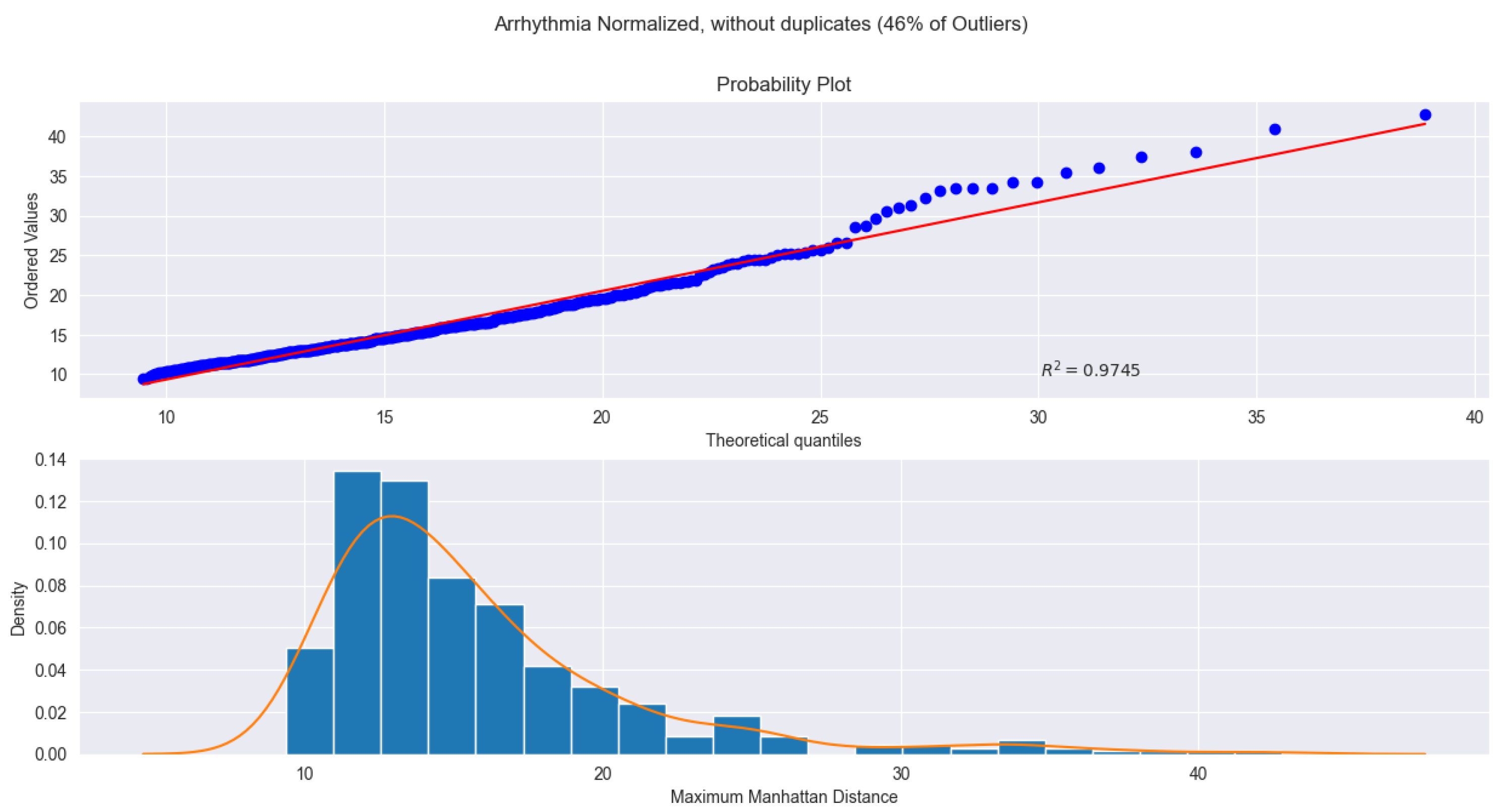
Figure 2.
Probability plot and histogram of the Parkinson dataset. Theoretical distribution for probability plot is set to skew-normal distribution after logarithmic transformation.
Figure 2.
Probability plot and histogram of the Parkinson dataset. Theoretical distribution for probability plot is set to skew-normal distribution after logarithmic transformation.
Disclaimer/Publisher’s Note: The statements, opinions and data contained in all publications are solely those of the individual author(s) and contributor(s) and not of MDPI and/or the editor(s). MDPI and/or the editor(s) disclaim responsibility for any injury to people or property resulting from any ideas, methods, instructions or products referred to in the content. |
© 2025 by the authors. Licensee MDPI, Basel, Switzerland. This article is an open access article distributed under the terms and conditions of the Creative Commons Attribution (CC BY) license (http://creativecommons.org/licenses/by/4.0/).
Copyright: This open access article is published under a Creative Commons CC BY 4.0 license, which permit the free download, distribution, and reuse, provided that the author and preprint are cited in any reuse.


