
Submitted:
20 October 2024
Posted:
21 October 2024
You are already at the latest version
Abstract
Outlier detection is a critical technique across various domains, including statistics, data science, machine learning, and finance. Outliers, data points that differ significantly from the majority, can indicate errors, anomalies, or even new insights. This article provides an in-depth exploration of the primary techniques used to detect outliers, categorized into statistical methods, machine learning-based approaches, and proximity-based methods. We discuss the advantages, limitations, and specific use cases of each technique, highlighting their applicability to different types of datasets. The goal is to equip practitioners with a better understanding of how to identify and handle outliers effectively in real-world data analysis.
Keywords:
1. Introduction
1.1. Outlier Detection
1.2. The Importance of Outlier Detection
- 1.
- Model Integrity: Outliers can skew results in machine learning models, leading to inaccurate predictions or biased estimations (Aggarwal, 2017). For instance, outliers may cause overfitting, where the model becomes too attuned to anomalies rather than representing the overall data structure accurately (Hodge & Austin, 2004).
- 2.
- Data Cleaning: In many cases, outliers are due to data errors, such as sensor malfunctions or incorrect data entries. Identifying and removing these outliers is crucial to improving the quality of the dataset, which in turn enhances the performance of machine learning algorithms (García et al., 2016).
- 3.
- Anomaly Detection: Sometimes, outliers represent meaningful anomalies rather than noise. Detecting these can lead to crucial insights, such as identifying network intrusions in cybersecurity or detecting disease outbreaks in healthcare data (Chandola, Banerjee, & Kumar, 2009). These examples illustrate the value of outlier detection in real-world applications, where finding anomalies can drive business decisions or public health interventions.
1.3. Types of Outlier Detection Techniques
1.3.1. Statistical Methods for Outlier Detection
- A)
- Z-Score Method
- B)
- Boxplot and Interquartile Range (IQR)
- C)
- Machine Learning-Based Approaches
- D)
- Isolation Forest
- E)
- Support Vector Machines (SVM) for One-Class Classification
- F)
- Autoencoders
1.3.2 Proximity-Based Methods
- A)
- K-Nearest Neighbors (KNN)
- B)
- Local Outlier Factor (LOF)
1.4 Challenges in Outlier Detection
- A)
- High Dimensionality: As the number of features increases, the difficulty of detecting outliers grows. In high-dimensional spaces, traditional methods like Z-Score and IQR may fail to capture complex relationships between variables. Machine learning-based methods like Autoencoders and One-Class SVMs are more suitable in such cases, but they come with increased computational costs (Aggarwal, 2015).
- B)
- Scalability: Many proximity-based techniques, like KNN and LOF, suffer from scalability issues in large datasets because they require calculating distances between all points. Techniques such as Isolation Forest are better suited for large-scale applications due to their efficiency in handling vast amounts of data (Liu et al., 2008).
- C)
- Imbalanced Data: In many cases, outliers constitute a small portion of the dataset. This imbalance can affect the performance of certain algorithms, which may be biased toward detecting the majority class. Approaches like resampling, ensemble learning, or cost-sensitive learning can help address this issue (He & Garcia, 2009).
2. Methodology
2.1. Machine Learning Approaches for Outlier Detection
2.1.1 Isolation Forest
- A)
- Random Partitioning and Isolation
- Threshold for Anomalies
2.2. Support Vector Machines (SVM) for One-Class Classification
2.2.1 Mathematical Formulation
3. Autoencoders for Outlier Detection
2.3.1 Neural Network Structure
- Reconstruction Error
2.4. Hyperparameter Selection
4. Results
4.1. Outlier Detection Using Machine Learning Methods
4.1.1. Isolation Forest
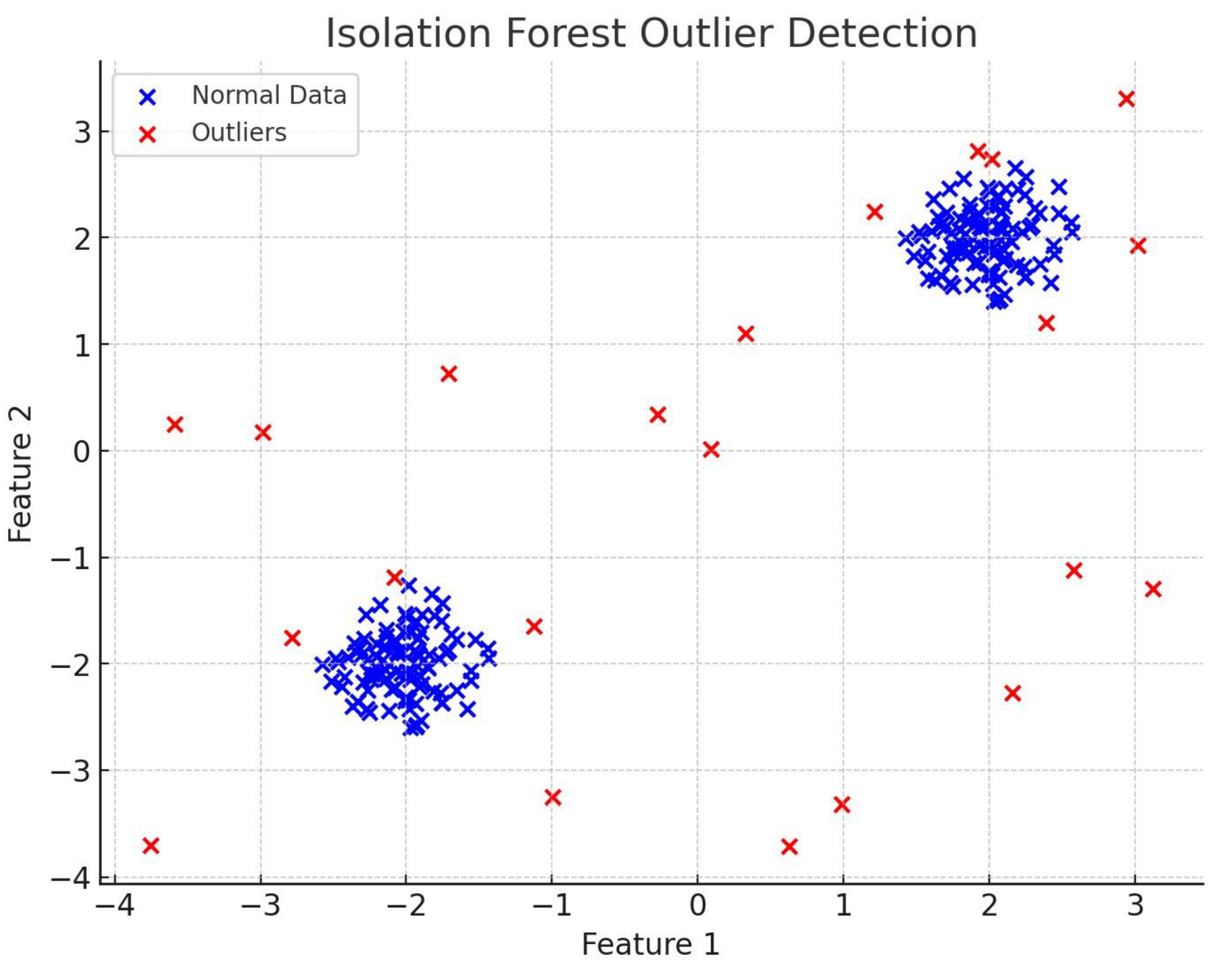
- Observations:
- Effectiveness: Isolation Forest performed well, detecting most of the outliers that were scattered around the edge of the feature space.
- Limitations: The performance is highly dependent on the contamination parameter, which determines the proportion of outliers. If this is not chosen carefully, the algorithm may misclassify normal data points as outliers.
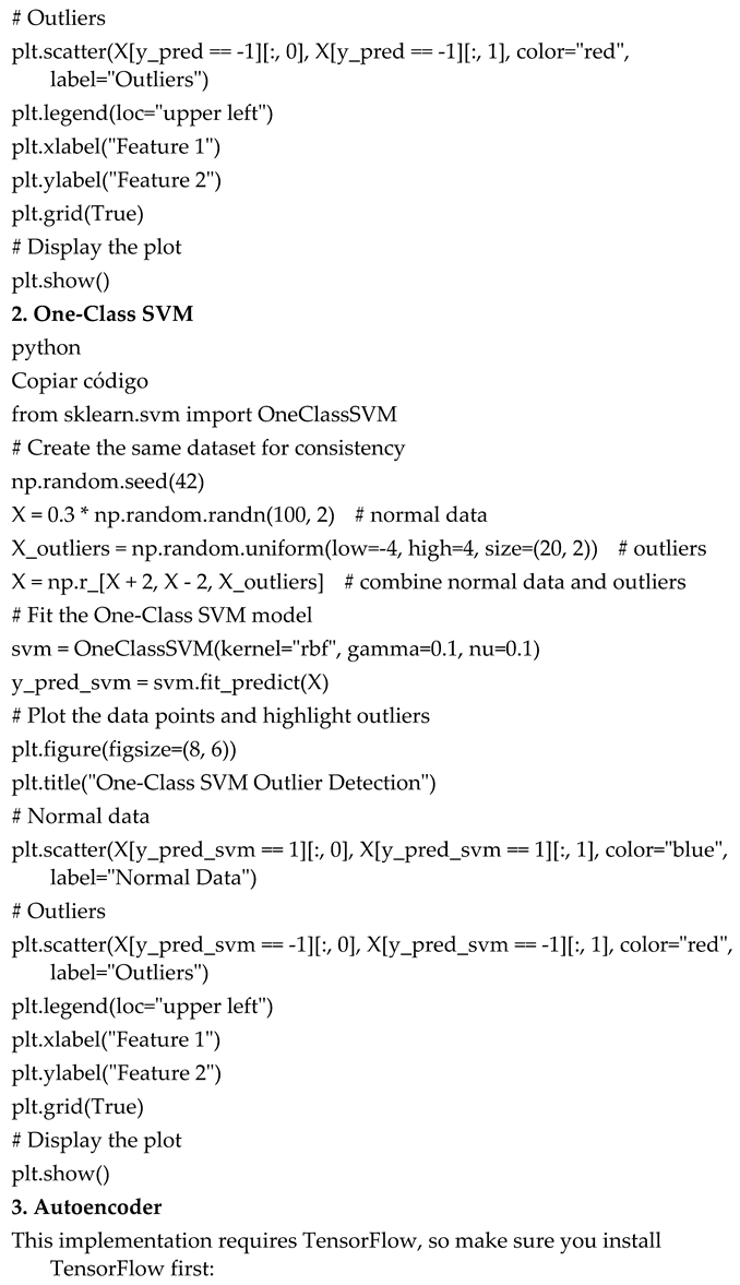
4.1.2. One-Class SVM
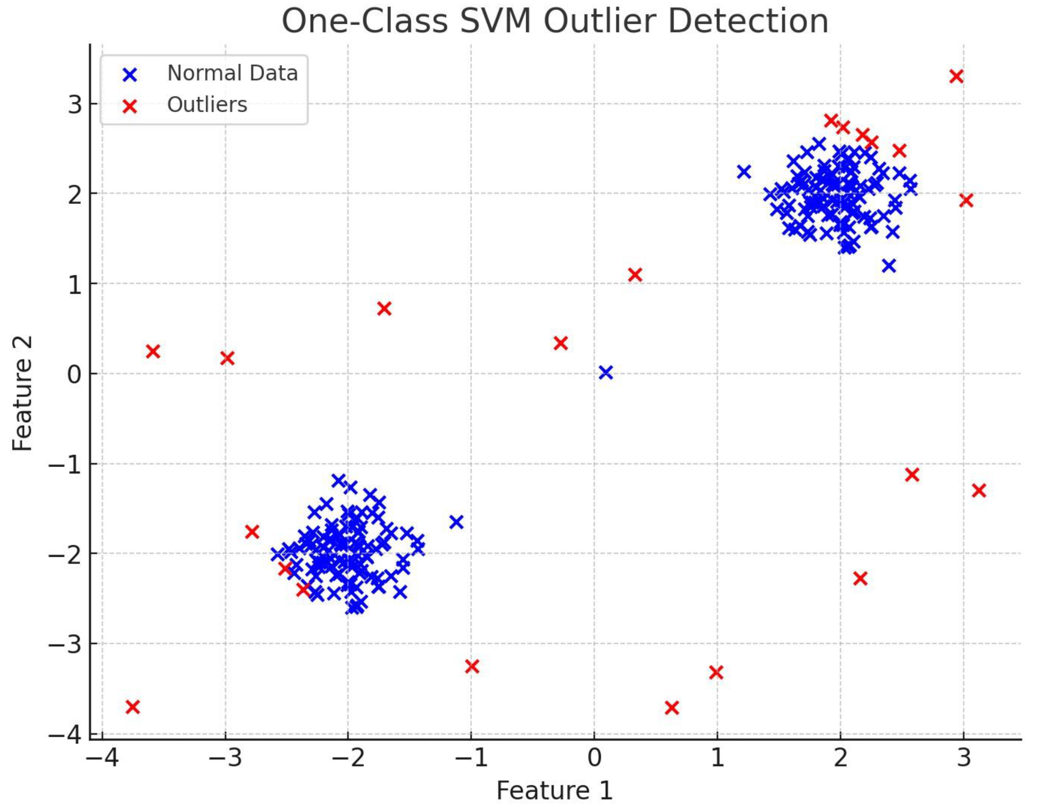
- Effectiveness: One-Class SVM performed well in detecting the outliers scattered around the dense clusters. The use of the RBF kernel helps capture the non-linearity in the dataset, improving accuracy.
- Limitations: One-Class SVM is sensitive to hyperparameters like the kernel parameter γ\gammaγ and ν\nuν, which controls the fraction of outliers. Adjusting these parameters is crucial for obtaining good results. Additionally, the computational complexity increases significantly for larger datasets.
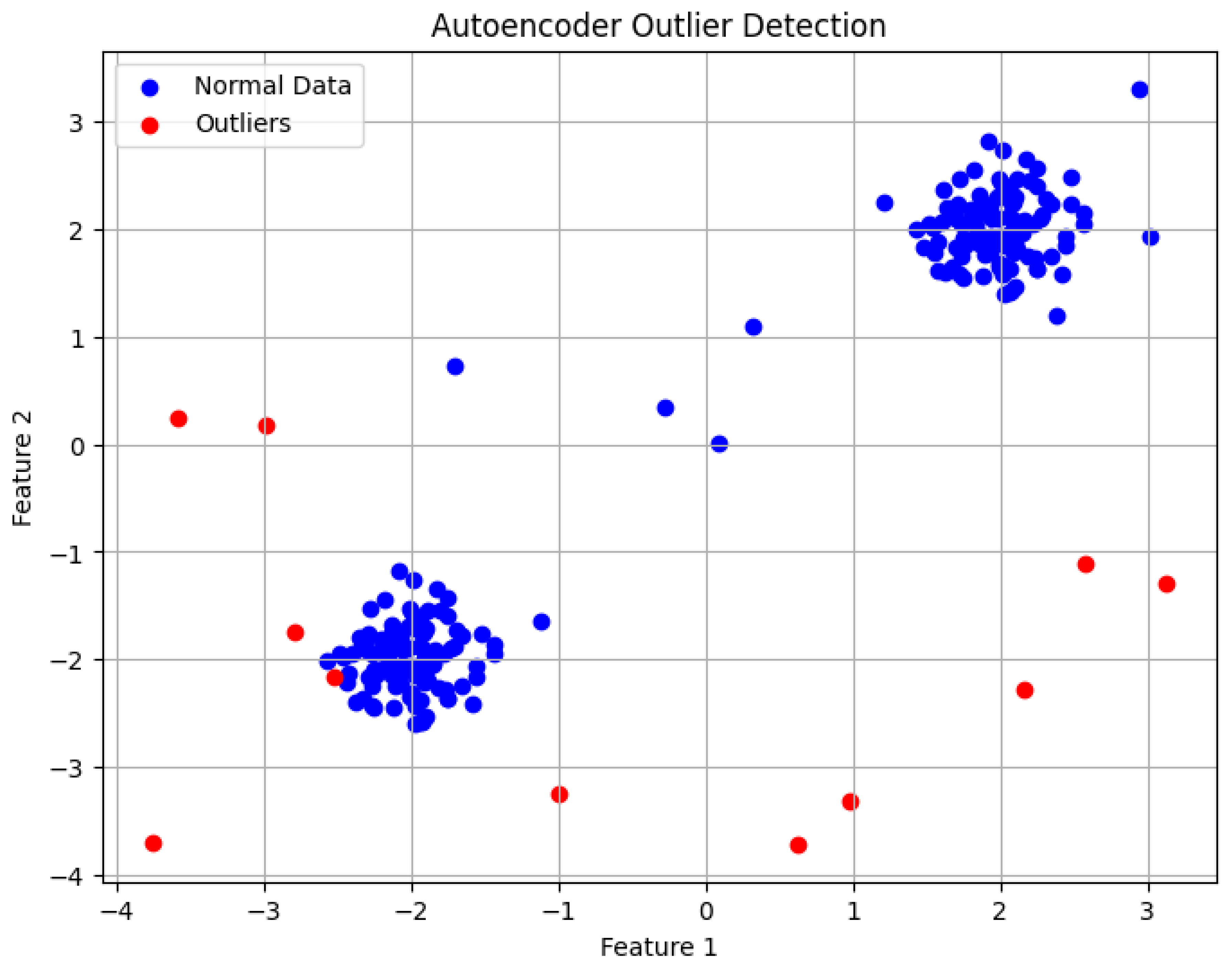
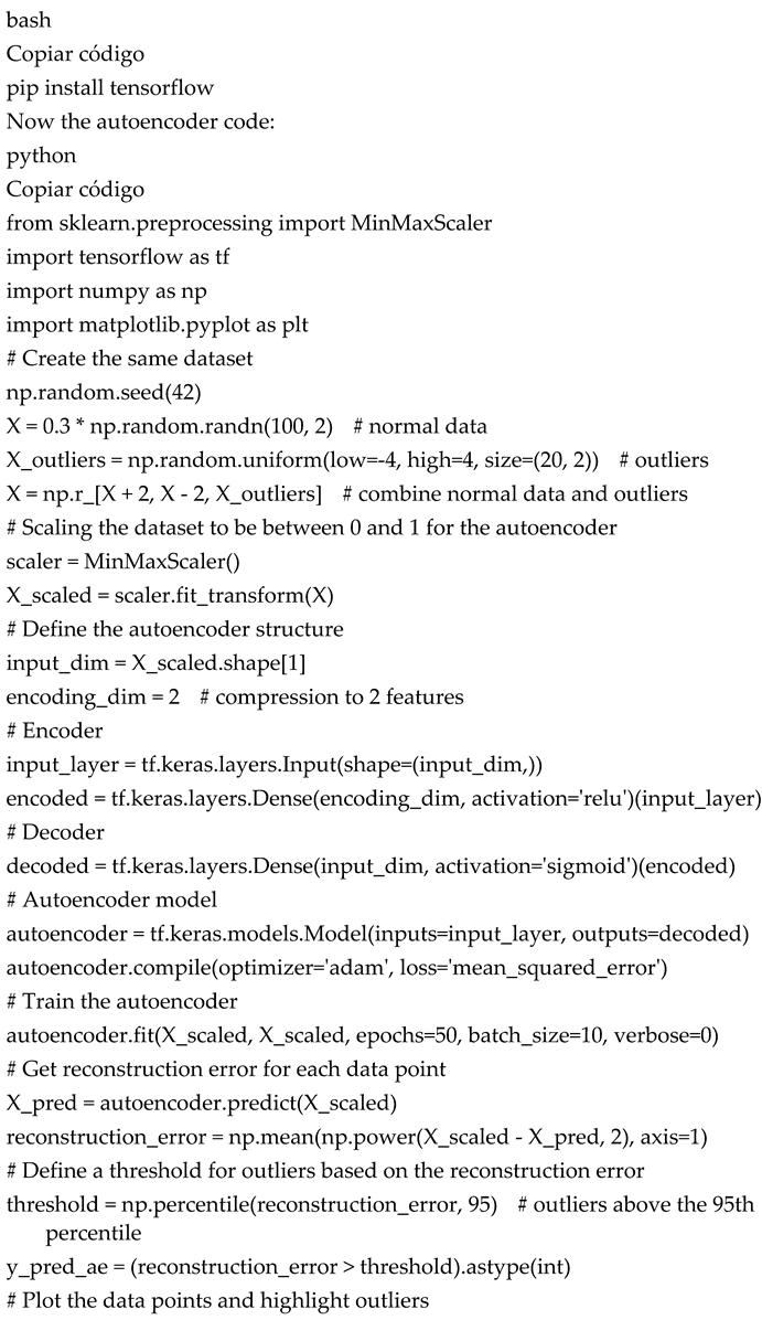
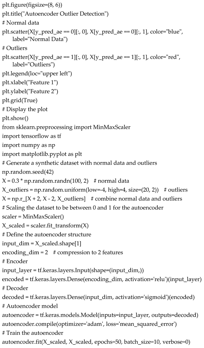
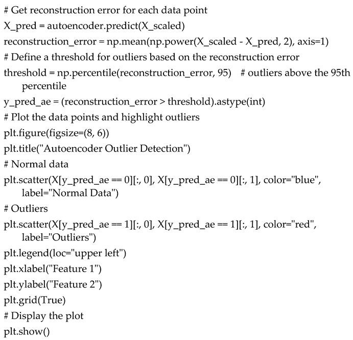
4.1.3. Autoencoder
- Observations:
- Effectiveness: The Autoencoder captured complex patterns in the data and accurately reconstructed normal data points. The model effectively identified outliers that differed significantly from the majority of the data.
- Limitations: Autoencoders require substantial amounts of data for training and are computationally expensive, particularly when dealing with high-dimensional data. Additionally, setting the threshold for reconstruction error is an empirical process that can vary depending on the dataset. Choosing a poor threshold can lead to false positives or missed outliers.
4.2. Summary of Results
- Isolation Forest: Random partitioning allows Isolation Forest to efficiently isolate outliers, making it suitable for large datasets with complex relationships.
- One-Class SVM: The ability to create a flexible boundary around normal data points makes One-Class SVM effective in high-dimensional or non-linearly separable data. However, it is computationally intensive and requires careful parameter tuning.
- Autoencoder: Autoencoders are powerful in identifying outliers by measuring reconstruction error, making them suitable for high-dimensional datasets. However, they are resource-intensive and require substantial training data.
- Each method has its strengths and is suitable for different use cases. Isolation Forest is ideal for large-scale applications, while One-Class SVM and Autoencoders offer advantages in high-dimensional datasets. The choice of method depends on the specific characteristics of the dataset and the application context.
5.Discussion
5.1. Comparative Analysis of Machine Learning Methods for Outlier Detection
5.2. Machine Learning Methods for Outlier Detection: Strengths and Weaknesses
5.2.1. Isolation Forest
5.2.2. One-Class Support Vector Machine (SVM)
5.2.3. Autoencoders
5.3 Practical Applications and Domain-Specific Considerations
5.3.1. Financial Fraud Detection
6. Conclusions
6.1. Summary of Findings
- Isolation Forest offers an efficient and scalable solution for large datasets, particularly when no assumptions about the data distribution can be made. Its strength lies in its ability to isolate anomalies based on recursive partitioning, making it an excellent choice for high-dimensional datasets. However, its performance is heavily dependent on the careful tuning of hyperparameters, such as the contamination ratio.
- One-Class SVM shines in situations involving high-dimensional and non-linearly separable data. The ability to leverage kernel methods allows One-Class SVM to construct complex boundaries that effectively separate normal data from outliers. However, its computational complexity and sensitivity to hyperparameters like ν\nuν and γ\gammaγ can limit its applicability in large-scale real-time environments.
- Autoencoders are highly effective in detecting anomalies in high-dimensional data, such as images and time-series datasets. By compressing data into a latent space and reconstructing it, autoencoders flag anomalies based on reconstruction error. While autoencoders are powerful tools, they require large datasets for training, considerable computational resources, and careful threshold selection for classification, which may pose challenges in certain practical applications.
6.2. Practical Implications
- The Author claims no conflicts of interest.
7. Attachments
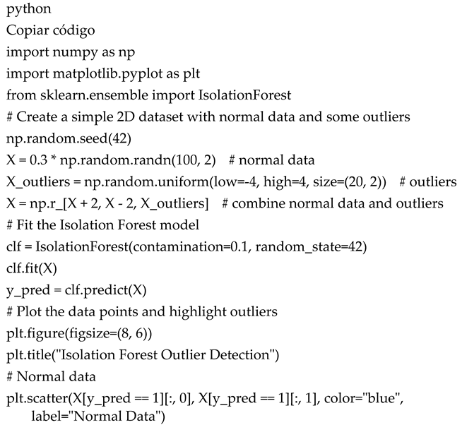
- Python Codes:
- 1.
- Isolation Forest
References
- Aggarwal, C.C. (2015). Outlier Analysis (2nd ed.). Springer.
- Aggarwal, C.C. (2017). Outlier Analysis. Springer.
- Bolton, R.J.; Hand, D.J. Statistical Fraud Detection: A Review. Stat. Sci. 2002, 17, 235–255. [Google Scholar] [CrossRef]
- Breunig, M.M.; Kriegel, H.P.; Ng, R.T.; Sander, J. LOF: Identifying density-based local outliers. ACM SIGMOD Record 2000, 29, 93–104. [Google Scholar] [CrossRef]
- Campos, G.O.; Zimek, A.; Sander, J.; Campello, R.J.G.B.; Micenková, B.; Schubert, E.; Assent, I.; Houle, M.E. On the evaluation of unsupervised outlier detection: measures, datasets, and an empirical study. Data Min. Knowl. Discov. 2016, 30, 891–927. [Google Scholar] [CrossRef]
- Chalapathy, R.; Chawla, S. Deep learning for anomaly detection: A survey. ACM Computing Surveys (CSUR) 2019, 54, 1–32. [Google Scholar]
- Eskin, E. Anomaly detection over noisy data using learned probability distributions. In Proceedings of the 17th International Conference on Machine Learning (pp. 255-262).
- García, S.; Luengo, J.; Herrera, F. Data Preprocessing in Data Mining; Springer International Publishing: Cham, Switzerland, 2016. [Google Scholar] [CrossRef]
- Hariri, S.; Kind, M.; Brunner, R.J. Extended isolation forest. IEEE Transactions on Knowledge and Data Engineering 2019, 33, 1479–1489. [Google Scholar] [CrossRef]
- Hodge, V.J.; Austin, J. A survey of outlier detection methodologies. Artificial Intelligence Review 2004, 22, 85–126. [Google Scholar] [CrossRef]
- Liu, F.T.; Ting, K.M.; Zhou, Z.H. (2008). Isolation forest. In 2008 Eighth IEEE International Conference on Data Mining (pp. 413-422). IEEE.
- Malhotra, P.; Vig, L.; Shroff, G.; Agarwal, P. (2016). Long short term memory networks for anomaly detection in time series. In Proceedings of the 23rd European Symposium on Artificial Neural Networks, Computational Intelligence and Machine Learning.
- Manevitz, L.M.; Yousef, M. One-class SVMs for document classification. Journal of Machine Learning Research 2001, 2, 139–154. [Google Scholar]
- Rudin, C. Stop explaining black box machine learning models for high stakes decisions and use interpretable models instead. Nat. Mach. Intell. 2019, 1, 206–215. [Google Scholar] [CrossRef] [PubMed]
- Schölkopf, B.; Platt, J.C.; Shawe-Taylor, J.; Smola, A.J.; Williamson, R.C. Estimating the Support of a High-Dimensional Distribution. Neural Comput. 2001, 13, 1443–1471. [Google Scholar] [CrossRef] [PubMed]
- Tax, D.M.; Duin, R.P. (2004). Support vector data description. Machine Learning 2004, 54, 45–66. [Google Scholar] [CrossRef]
- Tukey, J.W. (1977). Exploratory Data Analysis. Addison-Wesley.
- Hubert, M.; Vandervieren, E. An adjusted boxplot for skewed distributions. Comput. Stat. Data Anal. 2004, 52, 5186–5201. [Google Scholar] [CrossRef]
Disclaimer/Publisher’s Note: The statements, opinions and data contained in all publications are solely those of the individual author(s) and contributor(s) and not of MDPI and/or the editor(s). MDPI and/or the editor(s) disclaim responsibility for any injury to people or property resulting from any ideas, methods, instructions or products referred to in the content. |
© 2024 by the authors. Licensee MDPI, Basel, Switzerland. This article is an open access article distributed under the terms and conditions of the Creative Commons Attribution (CC BY) license (http://creativecommons.org/licenses/by/4.0/).


