
Submitted:
02 November 2025
Posted:
03 November 2025
You are already at the latest version
Abstract
The acceptance or rejection of a measurement is determined based on its associated measurement uncertainty. This decision-making process inherently carries the risk of errors, including the possible rejection of compliant measurements or the acceptance of non-conforming ones. This study introduces a mathematical model for the spatial evaluation of global risk to both producers and consumers, grounded in Bayes' theorem and with the application of a decision rule incorporating a guard band. The proposed model is well-suited for risk assessment within the framework of multivariate linear regression. The model's applicability was demonstrated through an example involving the flatness of the workbench table surface of the CMM. The least-risk direction on the workbench was identified, and risks were calculated under varying selections of the reference planes and differing measurement uncertainties anticipated in future measurement processes. Model evaluation was conducted using performance metrics derived from confusion matrices. The spaces of the most used metrics over the domain limited by the dimensions of the CMM workbench were constructed. Using the tested metrics, the optimal widths of the guard band were determined, which ensures the smallest values of the global producer's and consumer's risk.
Keywords:
spatial risk assessment
; global consumer’s risk
; global producer’s risk
; measurement uncertainty
; confusion matrix
; minimum zone
; coordinate measuring machine
1. Introduction and Basic Information
In today’s manufacturing environment, where every product must comply with established standards before reaching consumers, the assessment of product quality plays a critical role. Evaluating product conformity involves measuring one or more characteristic properties relevant to the product in question [1]. Under a simple acceptance decision rule, the measured value is compared against the permissible limits defined by the tolerance interval (). It is checked whether the measured value of the quantity of interest is within or outside the limits of the tolerance interval [2]. Decision-making becomes particularly challenging when the measured value lies near the boundaries of the tolerance interval, as this can lead to significant economic repercussions for both producers and consumers [3,4,5]. The risk and associated costs arise from mistakenly rejecting a compliant product whose measured value falls within the tolerance limits. Conversely, a product may be accepted as conforming to specifications even though it is not. These potential mistakes are quantified as specific risks for each characteristic property [6,7,8]. When multiple characteristic properties are considered, an overall total specific risk is calculated [9,10].
The measurement result and measurement uncertainty are inextricably linked. Measurement uncertainty refers to the range of values that can be assigned to a measurand [11]. The measured value, along with its associated uncertainty, is used to establish a guard band around the specification limits, with acceptance and rejection zones [12,13,14]. Incorporating a guard band into the conformity assessment process, the risk of making wrong decisions can be effectively controlled, assessed and reduced [15,16,17,18]. In this context, in addition to the tolerance interval, risk assessment also includes an acceptance interval (), which specifies the permissible upper and lower bounds for measured values [19,20]. In this study, closed tolerance and acceptance intervals were observed. Within the producer’s risk minimization framework, the tolerance interval is enclosed by the acceptance interval. Conversely, under the consumer’s risk minimization approach, the acceptance interval is contained within the tolerance interval [14,21,22]. In both models, the tolerance and the acceptance interval are separated by a guard band of width w. In the so-called shared risk model, the limits of the tolerance interval and the acceptance interval coincide.
By incorporating the measurement uncertainty of a future measurement process, a probabilistic model to assess risk is obtained based on Bayes' theorem, with the application of decision rules with a guard band [23,24]. The core concept of "point-based" risk assessment was adopted by the Joint Committee for Guides in Metrology (JCGM) and formalized in guide 106:2012 [19]. This procedure yields global producers' and consumers' risks for a single value within the tolerance interval and acceptance interval. Global producer’s and consumer's risks are obtained by combining information about possible, assumed values that the quantity being measured can take with data obtained from future measurements. The true value of the product characteristic under measurement is treated as an unknown parameter associated with a prior probability distribution. Selection of this prior distribution follows the principle of maximum entropy (PME) and is guided by the nature of the measurand and available data sources [25,26,27,28,29,30]. Prior knowledge can be informed by historical measurement data, relevant standards, technical manuals, or expert judgement based on the measurer’s experience [31,32,33]. Essential inputs to define the prior include the best estimate of the measured quantity, denoted , and the corresponding measurement uncertainty, . Parameters of the prior distribution are estimated using techniques such as the method of moments or maximum likelihood estimation, leveraging information from and [19,34,35]. Depending on the number of available data (both and , only , or none), the prior can be represented as a two-parameter, one-parameter, or non-parametric distribution [25,35,36]. Measurement values obtained in the future are modeled via a likelihood function, which requires as input the measurement uncertainty, associated with the anticipated measurement process.
The point-based approach for risk estimation, as delineated in Guide 106:2012, yields a single, definitive value for both the global producer's risk and the global consumer's risk [19]. This assumes determining the risk for exactly one value of the best estimate . It is used for risk quantification and quality assessment of various products, such as food, water, pharmaceuticals, medical treatments, natural gas, fuels, and other industrial goods [37,38,39,40,41,42,43]. Quality assessment can also be performed for multiple characteristics of an item of interest [44,45,46]. In the case of multi-component quality control, the total risk of false decisions is calculated. This requires determining a guard band for each controlled component [47,48].
By discretizing a naturally selected domain and transforming the argument of the prior distribution in Bayes' theorem, this fundamental point-based method for risk assessment can be two-dimensionally and three-dimensionally extended. Assume the best estimate is fixed and placed within both the tolerance interval and the acceptance interval. It is not required that the position of the best estimate be centered within either the tolerance or acceptance intervals [49]. The , and denote the lower and upper limits of the acceptance interval of the global producer's risk minimization model, respectively. The notations and refer to the lower and upper limits of the acceptance interval of the global consumer's risk minimization model. Holds that , Figure 1.
Figure 1 shows an interval representation of the risk assessment domain along the guard band axis. This interpretation allows the construction of risk curves on the interval . Holds that . The two-dimensional extension of the point-based method for risk assessment given in JCGM 106:2012 is obtained by discretizing the interval [35,43,50]. Values of global consumer's and producer's risk are calculated in each point of subdivision. The limits of the acceptance interval change with the change in the width of the guard band so that it simultaneously holds that and . In this process, the values and for the lower and upper limit of the tolerance interval are fixed. It is shown that the curves of the global producer's risk along the guard band axis on the interval increase, while the curves of the global consumer's risk at the same time decrease [43,50,51,52].
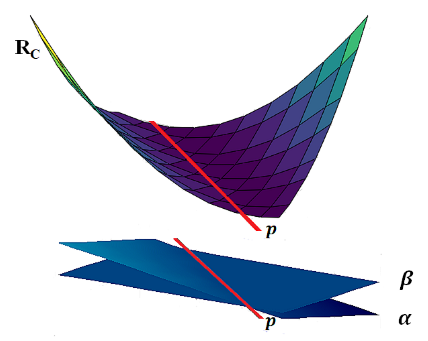
In addition to the previously discussed extension, the point-based method for risk assessment can be two-dimensionally extended in a manner that the arguments of prior distribution are functionally related data. This approach is applicable for regression and calibration, allowing the construction of risk curves along the moderate scale [52,53,54]. Risk assessment in regression is carried out naturally, considering the line . When the regression line intersects line, the resulting risk curves on the moderated scale take the form of upward-opening parabolas, with their minima located at the intersection points [52]. If the regression line coincides with or runs parallel to , the risk curves become linear and run parallel to the axis of the moderated scale [55]. Calibration risk assessment models are derived from these regression-based risk frameworks [53]. These models require defining tolerance and acceptance intervals for the explanatory variable corresponding to the given values of the response variable [53,54]. Within the domain enclosed by the interval on the guard band axis and with an interval on the moderate scale, it is possible to observe the surfaces for global consumers' and global producers' risk in both regression and calibration settings [52,53,54].
In this study, a step further has been taken. This study presents an advancement in risk assessment methodology by introducing a three-dimensional extension of the point-based approach. The method enables spatial risk assessment and is suitable for application in the case of multiple linear regression, resulting in the construction of a 3D risk space. The extension is demonstrated through a practical example involving the risk assessment of a plane that was determined in estimating the flatness error of a coordinate-measuring machine (CMM) worktable. This control is important because deviations in the flatness of the CMM worktable from the limits specified by the manufacturer can significantly affect the measurement results in procedures such as calibration of standards, measuring equipment, etc. [56]. The equation of the plane through the sampled points was determined using the minimum zone (MZ) method. Several variants of the MZ method are prevalent in practice [57]. In this study the One Point Plane Bundle Method (OPPBM) was used, which identifies an optimal plane through the sampled points, minimizing the distance between points with the most extreme values measured [58]. The method is recommended by the ISO 1101:2017 standard for verifying form errors within a specified zone [59]. The risk space was defined by the coordinates of sampled points of the CMM worktable, whose flatness is being assessed. The third axis of the risk space is represented by the values of the global risk of producers and consumers computed at subdivision points of the interval , as illustrated in Figure 1.
The spatial risk assessment model was evaluated using confusion matrix-based metrics. There are four possible outcomes in conformity assessment of a product with the required specifications, Figure 2.
The true value (TV) of a characteristic property of an item of interest may fall within the tolerance interval, while the measured value (MV) may fall within the acceptance interval. This is related to the valid acceptance of measurements, i.e., the probability of true positive values (TP), in the conformity assessment process. If the MV falls outside the acceptance interval, assuming that the TV is outside the tolerance interval, a valid rejection of the measurement occurs, resulting in a true negative probability (TN). If the MV of a property of an item of interest is within the acceptance interval, but the TV of that property is assumed to fall outside the tolerance interval, this results in a global consumer's risk (Rc) or false acceptance probability (FA). A scenario where MV is outside the acceptance interval while the TV is within the tolerance interval represents the global producer's risk (Rp) or the probability of false rejection (FR) [19,35,51].
2. Materials and Methods
2.1. Measurement Description
The granite surface of a CMM worktable can be mechanically damaged during exploitation. This can significantly affect the accuracy of measurements taken with the given device [56,60,61]. The risk of measurements on the CMM worktable concerning the flatness of its granite surface was assessed in this study. Measurements were conducted at the Department of Production, Faculty of Technical Sciences, University of Novi Sad, by using a CMM device whose worktable surface is the object of interest. A Carl Zeiss Contura G2 CMM with an RDS rotating head and a VAST XXT passive measuring sensor was used. With this CMM, measurements can be performed in the range of 1000×1200×600 mm. According to the manufacturer's specifications, the maximum permissible error is µm. The value for L is given in mm. The measurement was performed with a silicon nitride (SiN) probe with a single tip, 5 mm in diameter and 75 mm in body width [56]. Sample collection was carried out at measurement sites, and measurements were collected point by point. Three measurements were performed at each of the sample points. The coordinates of the sampled points of the granite table of the CMM and the mean value calculated for three measurements for the flatness of the surface along the z-axis are given in Table 1 in [56]. The coordinate values of the sampled points and the values for the surface flatness in that table are given in millimeters.
2.2. Best Estimate and Measurement Uncertainty
The equation of the plane of the granite table of the CMM was determined based on the measurements given in Table 1 in [56]. The software solution for determining the plane using the MZ method was developed at the Faculty of Technical Sciences in Novi Sad [58]. The equation is of the form and is given by the expression:
The parameters A, B, and D in equation (1) are given in millimeters. One of the input parameters of the model for estimating the global producer's risk and the global consumer's risk is the best estimate of an item of interest. In this case, the best estimate is represented as an n-tuple whose components are obtained by inserting the coordinates of the sampled points into equation (1). For simplicity, the notations for the components of the best estimate were introduced. The global producer's risk and global consumer's risk are computed for each value For the calculation of global producer's risk and global consumer's risk, the point-based method for risk assessment is still used, but the functional relationship of the data given by equation (1) is considered. The measurement uncertainty associated with the best estimates is the same for all sampled points and is . This measurement uncertainty is determined according to research [62,63].
Each observed point , near the regression plane is assumed to be a realization from a normal distribution centered at the predicted value of the regression plane. Therefore, the prior has the form .
The measurement uncertainty required for the definition of the likelihood function is determined in the future measurement process, independently of the current procedure used to derive the plane from equation (1). The likelihood function of a measured quantity value , with a given value is also modelled as a normal distribution and holds that [19]. It is presumed that the measurement uncertainty of a future measurement process controlling the quality of the CMM granite worktable, after exposure to exploitation, has a value . In addition to the stated values, the study also provides a comparison of risks for the scenarios where and
2.3. Selection of the Reference Plane
The assessment of global producer's and consumer's risk for the linear regression model is conducted in relation to the line [52]. The estimate provides the risk of the regression line deviating from the line. The line naturally imposes itself as a reference line for risk assessment in linear regression models because it represents an ideal measurement. In this study, for spatial risk assessment purposes, it is assumed that data are functionally connected by a multiple linear regression model. However, in this instance, there is no inherent reference plane to serve as a benchmark for evaluating risk. Therefore, that plane must be defined. Since the risk is determined in the process of assessing the flatness of a surface, the reference plane is assumed to be parallel to the xy-plane. Considering that the MZ method was employed to derive the equation for the flatness testing of a granite table, the plane taken as the reference plane is as follows:
where is mm, mm, and is the value of a reference plane. The choice of plane from equation (2) is based on the process of determining the equation of the plane using the MZ method. The reference plane is established through the center point of the parallelogram defined by the maximum and minimum value of measured surface flatness reported by a CMM [58].
2.4. Tolerance Plane and Acceptance Plane
In spatial risk assessment, the role of tolerance intervals and acceptance intervals is taken over by tolerance planes and acceptance planes. The tolerance space is bounded by the lower tolerance plane and the upper tolerance plane . These two planes are parallel to the plane as well as to one another. Since it is a class 0 granite surface plate, the width of the tolerance space is equal to μm [64]. For each value the upper tolerance plane has the equation mm, and the lower tolerance plane has the equation mm. The width of the acceptance space in the model of minimization of global producer's risk is equal to . In the model of minimization of the global consumer's risk, the width of the acceptance space is . The discretization of the domain along the guard band axis is carried out by introducing the multiplicative factor of the form An interval subdivision method was performed with a step of 0.1. This leads to subdivision nodes. A finer step would increase the number of nodes. However, it is shown that a subdivision step of 0.1 is sufficient for determining the global producer's and consumer's risk, and the obtained risk surfaces are sufficiently smooth. The subdivision nodes of the interval are of the following form:
where µm is the total width of the guard band. The acceptance planes for fixed values of and are calculated from the following equations:
The index in equations (4-5) for the values of the lower and upper limits of the acceptance interval indicates that the interval refers to the points , and it holds that and for each .
For it is true that , i.e., and . These are the conditions of the model of minimization of the global producer's risk. For it is true that , i.e., and . This therefore represents a shared risk model. If then . This represents a model of minimization of global consumer's risk, so that and . To maintain simplicity, only the value of the multiplicative factor will be provided in the subsequent text without referencing the index . The plane and the reference plane together with the tolerance planes and and the acceptance planes mm and mm, , are shown in Figure 3.
Figure 3 illustrates the model of minimizing global consumer risk with linearized geometry. A model of minimization of global producer's risk can be presented similarly. The line highlighted in red represents the intersection of planes and . The equation of that line is given by:
The points of the line are the only points of the plane that are exactly in the middle of the tolerance field and the acceptance field [49]. It should be noticed that the plane α on the domain defined by the plane in which the sampled points lie does not intersect the tolerance planes or acceptance planes anywhere. This indicates that the model will not exhibit anomalies that may arise when such a mutual relationship between the tolerance and acceptance planes and the regression plane is present [52].
2.5. Risk Calculation
Considering the previously defined model parameters, assuming that the prior function and the likelihood function are normally distributed, the global consumer's risk in linear multivariate regression case, at each measurement point , for each associated best estimate value , can be calculated from the equation:
The global producer's risk is calculated from the equation:
In equations (7–8) denotes the standard normal probability density function (PDF). The expression is given by the equation:
The symbol in equation (9) stands for the cumulative distribution function for the normal distribution (CDF). Equation (9) and the integrals in equations (7–8) were obtained by transforming the argument of the prior in the point-based risk assessment method and by discretizing the constructed domain [19]. In transforming the prior argument, the functional connection of the data, given by equation (1), is considered. Since the function from equation (1) is continuous at the points and is continuous in the arguments from equation (9), the data obtained from equations (7–8) must also be functionally connected by a continuous function. The integrals from equations (7–8) were solved numerically. This was accomplished using packages from the R programming language [65,66]. The graphs were created using either R or Octave software [67].
3. Results
3.1. Risk Curves
Although it may happen that the measurement values for the flatness of the surface at points are equal, the resulting risks do not have to be equal. The values of global consumer's risk shown in Figure 4a correspond to the measured surface flatness values listed in Table 1 of [56] for . The flatness of the surface of mm was measured at three different locations on the worktop of the CMM table, but the associated risks for these measurements, highlighted in red, vary. The representation in Figure 4a is given for the measured values of surface flatness before smoothing the data with the regression plane . When the risk is presented considering the functional relationship of the data described by the equation of the plane , it becomes evident that the risk values highly depend on the position of the sample points . The dependence is expressed relative to the line from equation (6), and relative to the plane in which the line lies. Figures 4c and 4d illustrate the curves of global consumers' and producers' risk along the axis representing the values of the regression plane α calculated at the points . These curves are upward-opening parabolas which have a minimum at a point that matches the value of the reference plane β from equation (2). Points that are equidistant from the axis of symmetry of the parabola, i.e., from the value specified in equation (2), have equal risks.
The curve that represents the global producer's risk increases along the guard band axis, while the curve of the global consumer's risk decreases along the guard band axis, Figure 4b. The curves shown are calculated for the value of the plane . For that value, the risks are the lowest, so the curves in Figure 4b are referred to as curves of minimum. The curves of minimum intersect each other for . The risk values are then . On these curves, the points corresponding to the risk values when , and are particularly highlighted. The highlighted points have the same value as the points of minimum of the parabolas shown in Figures 4c, d. If , the guard band width values of the guard band width shown in Figure 4b are negative, corresponding to the conditions for a model that minimizes the global producer's risk. The values and indicate that it is a shared risk model. For , it holds that . This represents the conditions for the model of minimization of global consumer's risk.
3.2. Risk Surfaces
The risk surfaces displayed in Figure 5a are the outcome of the three-dimensional extension of the standard, point-based method for risk assessment.
The risk surfaces presented in Figure 5a are displayed within the domain defined by the interval on the guard band axis, and the range of measured values for surface flatness . The maximum values of both the global producer's risk and global consumer's risk occur at the boundaries of interval . The maximum values of the global producer's risk along the guard band axis are achieved for . Simultaneously, the values of the global consumer's risk are minimal, Figure 5b. The risk surfaces in Figure 5a include the curves of minimum depicted in Figure 4b. All results analyzed so far obtained through the spatial risk assessment method are consistent with the results of previous research [43,51,52].
In Figure 4b, among others, the points for which are particularly highlighted. The global producer's risk along the guard band axis is then the highest and amounts to . Concurrently, the global consumer's risk along the guard band axis is at its minimum, with a value of . Figures 6a and 6b illustrate the risk surfaces for . In contrast to the risk surfaces shown in Figure 5a, these surfaces are displayed within the domain. The interval lies on the x-axis, while is the interval on the y-axis. The lines and highlighted in Figure 6a and 6b pass through the points and respectively. The value of the variable for a given is obtained from equation (6). The orthogonal projections of the lines and onto the xy-plane have the same direction and position as the projection of the line onto the xy-plane. This orthogonal projection of the line onto the xy-plane is hereinafter denoted by The risk of flatness deviation of the CMM worktable surface from the specified standards is smallest in the direction of line , Figure 6c. On the domain, the risks are greatest at the point of the CMM workbench with coordinates . At that point the risk values are and .
The risk surfaces displayed in Figure 5a and Figure 6a,b have different domains. The depiction of the risk surface on the domain enables the identification of the minimum curves along the guard band axis and the assessment of the surface flatness value that yields the lowest risks. The representation of the risk surfaces on the domain has a practical application. This representation illustrates how to position the measurement object on the workbench surface so that the flatness of the surface and potential damage to the CMM device's workbench surface have the least impact on the measurement results.
3.3. Risk Spaces
Risk surfaces on the domain can be obtained for each . The global producer's risk space and the global consumer's risk space are formed by stacking these layers on top of one another, Figure 7a,b.
The stacking of the consumer's global risk layers concerning the multiplicative factor is descending. For , holds . The construction of the global producer's risk space is ascending. For , holds . The minimum of each layer is along the direction of line . The global consumer's risk space reaches its maximum at point A, with , and it has a value of . As the behaviors of global producer's and consumer's risks are reversed, the maximum of the space of global risk of producers is reached at the same point, but for and amounts, as already stated, to . It should be noticed that the spatial risk assessment method allows risk assessments for any guard band width and at locations where surface flatness measurements have not been made.
In this multivariate linear regression model, the output variable depends on two input variables and . A representation of risk assessment in a model with more than two input variables would be given through combinations of pairs of variables.
3.4. Dependence of the Results on the Choice of the Reference Plane
This study presents the spatial risk assessment method for the first time. Therefore, there is currently no established professional consensus regarding the selection of the reference plane . The choice of reference plane in this context is specific, as it is derived from the MZ method. The reference plane was determined based on the extreme values obtained from the surface flatness sample. In some problems, such values would be discarded as outliers and excluded. Thus, when selecting a reference plane for multiple linear regression models, it is advisable to use the sample mean or another relevant value, depending on the specific practical problem being addressed. In this case, there is no significant difference between the mean value of the data mm and the value taken by plane Therefore, the difference in risks is minimal, Figure 8d,e. When this disparity is substantial, there are also discernible differences between the estimated values for producers' and consumers' global risk.
Figure 8 illustrates the variations in values of global consumers' and producers' risk for and different choices of reference planes. The values of the reference planes are selected to match the characteristic points of the surface flatness sample: (a) minimum value, mm, (b) mode1, mm, (c) mode2, mm (d) median, mm, (e) MZ method, the value taken by the plane mm, (f) mean, mm, (g) maximum value, mm. As the reference plane values shift from minimum to maximum, the region indicating the highest global consumer or producer risk transitions from point A on the workbench surface to the lower-left corner. It is essential to highlight the centrally symmetrical relationship between the graphs when the minimum and maximum surface flatness values are used as reference planes, Figure 8a and 8g. The least-risk direction and position correspond to case (e), where the reference plane is derived from the MZ method. This direction and position also correspond to the direction and position of the line Considering a line that would be the intersection of plane α and any chosen reference plane, its projection onto the xy-plane would be parallel to line .
3.5. Dependence of Results on Measurement Uncertainty
Risk calculation requires information about the prior distribution and the measurement uncertainty, , of a future measurement process. The spatial risk assessment method allows for the prediction of the risk value for the desired measurement uncertainty even without performing a measurement. All results so far are calculated for . Figure 9 shows a comparison of the risk space from Figure 7 with the spaces obtained for and To facilitate comparison, the risk space is projected onto a plane to which the line is perpendicular. The observed lattice of space is limited by the layers obtained for and . The vertical lines on the graphs correspond to the lines connecting the layer vertices.
The space of global consumer’s risk contracts as measurement uncertainty increases. The values of the global consumer's risk for the layer of space where increase. Simultaneously, the values of global consumer's risk for the risk layer where are declining. As a result of the change in the value of measurement uncertainty , the increase in the risk values of the lower layer is significantly more pronounced than the decline in the risk value of the upper layer of the space of global consumer’s risk, Figure 9.
The contraction of the space of global consumer’s risk cannot be observed independently of the behavior of the space of global producer’s risk. With the increase in measurement uncertainty , there is a translation of the space of global producer’s risk along the risk axis toward higher values, Figure 9. The space of the global producer’s risk expands until the point of alignment of the risk layers, that is, until the point at which the risk layers are almost parallel to the xy-plane. The critical value at which a change in the shape of the layers occurs is μm. That is approximately in terms of the tolerance field range. After the critical value, the layers of the space of global producer’s risk change shape in projection, from an upward-opening parabola to a downward-opening parabola. The space of global consumer’s risk is contracting, while risk values are rising. Although for the values of the global consumer's risk are below , the values of the global producer's risk are extremely high and go above 30%. Due to such unfavorable results for the producer, models that have a measurement uncertainty greater than the critical value should not be considered. If the method were used for quality control in the production of CMM granite worktables, under such conditions, the producer would have numerous non-compliant worktables and extremely high production costs.
4. Model Evaluation
4.1. Conformance Probability
To evaluate the model, the conformance probability is used. This is the probability that the item of interest, in this case, the flatness of the surface, is within the specification limits. For a measured value , outside the acceptance interval, conformance probability represents specific producer’s risk [19]. In machine learning terms, conformance probability represents the prevalence [68].
Evaluation of the model is required because the conformance probability may be small despite the risk values being small. These anomalies arise when a regression line or plane intersects a tolerance line or plane [52]. According to the two-dimensional interpretation of the risk assessment procedure depicted in Figure 2, the expression for calculating the conformance probability presented in [19] (p. 27) should be slightly redefined. Instead of the expression:
that can lead to misunderstanding, the next expression should be observed:
Applying transformations that are equivalent to those that are implemented in the calculation of the global producer's and consumer's risk [19,51], equation (11) takes the form:
Assuming that , for and by applying the following properties related to CDF:
it is obtained that equation (10) is valid for each and for each . From equation (10), it is obvious that the value for the conformance probability depends on the best estimate and its associated measurement uncertainty . Each value has the same width of tolerance space. Therefore, the values of conformance probability over the domain are the same for each , i.e., for each width of the guard band . The same applies to the values of conformance probability over the domain , Figure 10.
The line of maximum values on the domain passes through the points , where . The line of maximum values on domain follows the CMM workbench's least-risk direction of line and has the value . The line of displays the lowest value in the domain. On domain, the minimum is achieved at point A, where the risks are at their highest.
4.2. Confusion Matrix
The lines , , , and partition the area, representing possible values of TV and MV, into nine distinct fields, Figure 11a [69].
From Figure 11a, the definition areas for the quantities shown in Figure 2 can be reconstructed. Given that, as well as the definitions of , , TP and TN probabilities, it is simple to demonstrate that and . It also held that . The probabilities , , TP and TN represent the classes of the confusion matrix, Figure 11b [35,51]. By using the mentioned connections between the global producer's and consumer's risk, and conformance probability, in addition to the spatial representation of and classes, as shown in Figure 7, it is possible to construct spaces of classes TP and TN (Figure S1, S2).
4.3. Probability of Frequent and Rare Events
It is clear from the confusion matrix that another marginal probability can be constructed in addition to the conformance probability. This is the probability of frequent events . It represents the probability that the measured value is within the acceptance interval. The probability of rare events is defined as [69]. Assuming and applying the same procedure that shows that the expressions from equations (10) and (11) are equivalent, the following equation is obtained:
For each value of the multiplicative factor , a probability surface for frequent events is generated. By stacking these layers one on top of the other, the overall probability space for frequent events across the domain is obtained, Figure 12a. The stacking of the layers of space, concerning the multiplicative factor , is descending. For , holds . The probability of frequent events can also be represented on the domain, Figure 12b. The maximum probability of frequent events in both domains is . This value is achieved by the layer of the multiplicative factor , Figure 12a, i.e., under the conditions of the model of minimization of global producer's risk, Figure 12b.
A narrower spacing between the layers depicted in Figure 12a would be achieved by implementing a finer subdivision step of the interval . At point A, where the risks are highest, the probability of frequent events is lowest and amounts to on both domains. It should also be noted that, in machine learning terms, the probability of frequent events is also referred to as bias [68].
Given the stated range of values that have conformance probability and probability of frequent events, it can be inferred that the model performs satisfactorily on the provided data and that there are no anomalies in the model.
4.4. Curves, Surfaces and Spaces of Metrics Associated with the Confusion Matrix
The integration of all elements used in metrology for conformity assessment enables the evaluation of risk assessment models in multiple linear regression using metrics associated with confusion matrices [35,51].
Among the many tested metrics are the metrics that illustrate the relationship between the global producer's and global consumer's risk in relation to conformance and non-conformance probabilities, as well as the probabilities of frequent and rare events. In relation to the multiplicative factor , the stacking order of layers for the False Positive Rate (FPR) and False Discovery Rate (FDR) metrics is a descending (Figure S3, S5). These metrics compare global consumer's risk with non-compliant measurement and probability of frequent events, respectively. Given that the curves of global consumer's risk along the guard band axis fall, the descending order of layers for these two metrics was expected. This confirms the previously mentioned results. In contrast, the False Negative Rate (FNR) and the False Omission Rate (FOR) are metrics that compare the global producer's risk with conformance probability, i.e., probability of rare events; thus, the ascending order of layers was obtained (Figure S4, S6). There are no intersections of layers for any of the metrics listed. Therefore, their behavior is considered stable for each The metrics for model evaluation that are most often used in practice are Accuracy, Precision, Recall and Specificity [70]. In the field of metrology, imbalanced data are the outcome of well-conducted measurement. Consequently, the probability of the TP class in the confusion matrix is the dominant one. For assessing imbalanced datasets, the F1-score metric serves as an effective evaluation tool. As the harmonic mean of Precision and Recall, the F1 score provides a balanced measure of these performance indicators [71,72]. Among the metrics listed, Precision, Recall and Specificity have stable behavior, while Accuracy and F1 score have unstable behavior (Figures S7–S11). Unstable behavior refers to the intersection of metrics layers.
Additionally, spaces for several less common metrics have also been constructed. Negative predictive value (NPV) and Markedness (MK) show stable behavior with respect to the intersection of metrics layers (Figures S12, S13). Balanced Accuracy (BA), G-mean, Bookmarked informedness (BM) and Cohen's kappa coefficient are metrics with unstable behavior (Figures S14–S17). The ranges for values of the multiplicative factor, , for which stability in the behavior of tested metrics is achieved, are provided in the supplementary materials. These ranges are determined by observing all values of and identifying a domain without layer intersection.
The most pronounced unstable behavior was observed with the MCC and DOR metrics. The surfaces of these metrics on the domain are hyperbolic paraboloids, Figure 13a,b. A hyperbolic paraboloid is a translation surface that is created by moving one parabola over another. The surface of DOR is formed by translating a parabola with an opening upwards along a parabola with an opening downwards and have a classic saddle shape. The MCC surface is formed by translating a downward-opening parabola along an upward-opening one, with its orientation opposite to the DOR. In Figure 13a, b, translation parabolas are highlighted red. On the MCC surface, this parabola is a curve of the minimum, with a maximum value of . This value is achieved for and guard band width . The values of the TNR and NPV metrics can be very small (Figures S11, S12), which results in relatively low values of the MCC metric on the domain , Figure 13c [68]. For the DOR metric, the parabola along which the translation is performed is the curve of the maximum with a minimum value , achieved for and the guard band width of .
The surfaces of MCC and DOR metrics are generated in a variety of ways, and consequently, the creation of the space of these metrics on the domain differs. For the stacking of the MCC layers is ascending, i.e. for , holds . For the values taken by the layers of the MCC metric are descending with respect to the multiplicative factor and it holds that . Here, the ascending and descending orders of the MCC minimums are discussed because the layers of MCC intersect at the edges of the domain , Figure 14a, 14c.
The MCC layers' minima lie on the curve of minimum highlighted red, Figure 13a. The red vertical lines in Figures 16a and 16c connect the stability area, i.e. the area where there is no intersection of layers. The stability area is achieved for .
For the DOR metric, the situation is reversed. If it holds , a descending trend in the values of the maximums of the DOR layers is clear. For , the maximums of the DOR layers are ascending. Therefore, the layers of the DOR metric also intersect each other, Figure 14b, d. The maximum values of the DOR layers lie on the curve of maximum highlighted red, Figure 13b. Unlike the MCC metric, if all are considered, the DOR metric does not have a stable area on the domain , Figure 14d.
The stable behavior of the tested metrics on the domain can be ensured by choosing the range of the multiplicative factor , for which the injectivity property is fulfilled in the sense that Labels and stands for values of the corresponding tested metrics calculated for given values of the multiplicative factor . The values , of the multiplicative factor, which ensures the injectivity of the tested metrics, are displayed in Table 1.
The guard band widths from Table 1 are calculated from the following equations: and . For the metrics Cohen’s kappa coefficient, MCC, and DOR, it is possible to determine two distinct intervals without intersection of the layers of the metrics. These intervals are separated and marked with L and R, Table 1. Both boundaries of the injectivity intervals, 6L, 7L and 8L, fall within the domain of the model of minimization for global producer's risk and represent the value of . For that reason, their guard band widths are within the range given in Table 1, while the width of the guard band does not exist. Similarly, both limits of the interval 8R are within the domain of the model of minimization of consumer's global risk and represent the value of . Consequently, the guard band does not exist, and the guard band is defined by the range provided in Table 1.
In addition to the injectivity intervals for individual metrics, it is also possible to determine the common injectivity interval, of all tested metrics, where the layers of metrics do not intersect. Three possible outcomes are outlined in Table 2.
Intervals and are situated within the domain of the model for minimizing the global producer’s risk, while interval is in domain of the model for minimizing the global consumer’s risk. Since the curves of minimum for global producer's and consumer's risks intersect for µm, Figure 4b, 5a, on the interval holds . The same applies to interval , while for interval it holds . Choosing interval achieves the smallest values of global producer risk and choosing interval achieves the smallest values of global consumer risk. In this manner, optimal guard band widths were obtained.
5. Conclusions
This study introduces a spatial risk assessment method based on a multiple linear regression model and demonstrates its application in the case of CMM workbench flatness. This method enables calculation of global producer's and consumer's risks even for locations where no direct measurements are taken and for any value of the guard band width . Through the case study, the least-risk area of the workbench surface was identified, and a critical measurement-uncertainty threshold was established, marking the point at which the global producer's risk landscape changes significantly. In addition, it is shown that by evaluating the model using metrics associated with confusion matrices, it is possible to determine the optimal width of the guard band.
With an appropriate selection of the reference plane, the method can be extended to risk assessment scenarios involving any input data type that can be represented through multiple linear regression. Consequently, this spatial risk assessment framework is applicable beyond metrology, offering potential utility across diverse scientific disciplines.
Supplementary Materials
The following supporting information can be downloaded at the website of this paper posted on Preprints.org, Figure S1: True positive; Figure S2: True negative; Figure S3: False positive rate; Figure S4: False negative rate; Figure S5: False discovery rate; Figure S6: False omission rate; Figure S7: Accuracy; Figure S8: Precision; Figure S9: Recall; Figure S10: F1 score; Figure S11: True Negative Rate; Figure S12: Negative Predictive Value; Figure S13: Markedness; Figure S14: Balanced Accuracy; Figure S15: G-mean; Figure S16: Bookmaker informedness; Figure S17: Cohen’s kappa coefficient.
Author Contributions
Conceptualization, D.B.; methodology, D.B., B.Š. and B.R.; software, D.B., B.Š. and M.R.; validation, D.B., B.Š., B.R., M.R, and A.R.; formal analysis, D.B; investigation, D.B. and B.Š.; resources, D.B., B.Š. and M.R.; data curation, D.B., B.Š., A.R. and M.R.; writing—original draft preparation, D.B.; writing—review and editing, D.B., A.R and B.R.; visualization, D.B. and A.R.; supervision, B.R.; project administration, D.B.; funding acquisition, B.R. All authors have read and agreed to the published version of the manuscript.
Data Availability Statement
The original contributions presented in this study are included in the article. Further inquiries can be directed to the corresponding author.
Conflicts of Interest
The authors declare no conflicts of interest.
References
- Kuselman, I.; Pennecchi, F.R.; Da Silva, R.J.; Hibbert, D.B. IUPAC/CITAC Guide: Evaluation of risks of false decisions in conformity assessment of a multicomponent material or object due to measurement uncertainty (IUPAC Technical Report). Pure Appl. Chem. 2021, 93, 113–154. [Google Scholar] [CrossRef]
- Ortolano, G.; Boucher, P.; Degiovanni, I.P.; Losero, E.; Genovese, M.; Ruo-Berchera, I. Quantum conformance test. Sci. Adv. 2021, 7, eabm3093. [Google Scholar] [CrossRef]
- Biserka, R.; Horvatić Novak, A.; Keran, Z. Impact of the quality of measurement results on conformity assessment. In Proceedings of the 29th DAAAM International Symposium on Intelligent Manufacturing and Automation, Zadar, Croatia, 24–27 October 2018. [Google Scholar] [CrossRef]
- Dias, F.R.S.; Lourenço, F.R. Measurement uncertainty evaluation and risk of false conformity assessment for microbial enumeration tests. J. Microbiol. Methods 2021, 189, 106312. [Google Scholar] [CrossRef] [PubMed]
- ILAC–G8:09/2019. Guidelines on Decision Rules and Statements of Conformity. 2019. Available online: https://ilac.org/publications-and-resources/ilac-guidance-series/ (accessed on August 29, 2025).
- Sedeek, M.A.; Elerian, F.A.; Abouelatta, O.B.; AbouEleaz, M.A. Decision-making Approach to Reduce the Risk of Measurement Uncertainty for Product Size. Manosura Eng. J. 2024, 49, 2. [Google Scholar] [CrossRef]
- Allard, A.; Fischer, N.; Smith, I.; Harris, P.; Pendrill, L. Risk calculations for conformity assessment in practice. In Proceedings of the 19th International Congress of Metrology, Paris, France, 24–26 September 2019. [Google Scholar] [CrossRef]
- Koucha, Y.; Forbes, A.; Yang, Q. A Bayesian conformity and risk assessment adapted to a form error model. Meas:Sens. 2021, 18, 100330. [Google Scholar] [CrossRef]
- Pennecchi, F.R.; Kuselman, I.; Di Rocco, A.; Hibbert, D.B.; Sobina, A.; Sobina, E. Specific risks of false decisions in conformity assessment of a substance or material with a mass balance constraint–A case study of potassium iodate. Meas. 2021, 173, 108662. [Google Scholar] [CrossRef]
- Bettencourt da Silva, R.J.; Lourenço, F.; Hibbert, D.B. Setting multivariate and correlated acceptance limits for assessing the conformity of items. Anal. Lett. 2022, 55, 2011–2032. [Google Scholar] [CrossRef]
- BIPM, IEC, IFCC, ILAC, ISO, IUPAC, IUPAP, and OIML. Evaluation of measurement data — Guide to the expression of uncertainty in measurement. Joint Committee for Guides in Metrology, JCGM 100:2008. [CrossRef]
- Pendrill, L.R. Using measurement uncertainty in decision-making and conformity assessment. Metrologia 2014, 51, S206. [Google Scholar] [CrossRef]
- Separovic, L.; Lourenco, F.R. Measurement uncertainty and risk of false conformity decision in the performance evaluation of liquid chromatography analytical procedures. J. Pharm. Biomed. Anal. 2019, 171, 73–80. [Google Scholar] [CrossRef]
- Williams, A.; Magnusson, B. Eurachem/CITAC Guide: Use of Uncertainty Information in Compliance Assessment. 2021. Available online: https://www.eurachem.org/index.php/publications/guides/uncertcompliance (accessed on August 29, 2025).
- Xue, Z.; Mou, X.; Sun, H.; Cao, C.; Xu, B. A Protocol for Conformity and Risk Assessment of Pharmaceutical Product by High Performance Liquid Chromatography Based on Measurement Uncertainty. J. Sep. Sci. 2025, 48, e70158. [Google Scholar] [CrossRef]
- Separovic, L.; Simabukuro, R.S.; Couto, A.R.; Bertanha, M.L.G.; Dias, F.R.; Sano, A.Y.; Caffaro, A.M.; Lourenco, F.R. Measurement uncertainty and conformity assessment applied to drug and medicine analyses–a review. Crit. Rev. Anal. Chem. 2023, 53, 123–138. [Google Scholar] [CrossRef]
- Božić, D.; Runje, B.; Razumić, A. The Cost of Wrong decisions. In Proceedings of the 19th International Conference Laboratory Competence-Brijuni 2024, Brijuni, Croatia, 23–25 November 2024. [Google Scholar]
- Volodarsky, E.T.; Kosheva, L.O.; Klevtsova, M.O. Approaches to the Evaluation of Conformity Taking into Account the Uncertainty of the Value of the Monitored Parameter. In Proceedings of the 2019 IEEE 8th International Conference on Advanced Optoelectronics and Lasers (CAOL), Sozopol, Bulgaria, 6–8 September 2019. [Google Scholar] [CrossRef]
- BIPM, IEC, IFCC, ILAC, ISO, IUPAC, IUPAP, and OIML. Evaluation of measurement data — The role of measurement uncertainty in conformity assessment. Joint Committee for Guides in Metrology, JCGM 106:2012. [CrossRef]
- Volodarskyi, Y.; Kosheva, L.; Kozyr, O. Reducing the Impact of Measurement Uncertainty in Conformity Assessment. In Proceedings of the 2023 XXXIII International Scientific Symposium Metrology and Metrology Assurance (MMA), Sozopol, Bulgaria, 7–11 September 2023. [Google Scholar] [CrossRef]
- Runje, B.; Horvatić Novak, A.; Razumić, A.; Piljek, P.; Štrbac, B.; Orošnjak, M. Evaluation of Consumer and Producer Risk in Conformity Assessment Decision. In Proceedings of the 30th DAAAM International Symposium “Intelligent Manufacturing & Automation”, Zadar, Croatia, 23–26 October 2019. [Google Scholar] [CrossRef]
- Hibbert, D.B.; Korte, E.H.; Örnemark, U. Metrological and quality concepts in analytical chemistry (IUPAC Recommendations 2021). Pure Appl. Chem. 2021, 93(9), 997–1048. [Google Scholar] [CrossRef]
- Lira, I. A Bayesian approach to the consumer’s and producer’s risks in measurement. Metrologia 1999, 36, 397. [Google Scholar] [CrossRef]
- Volodarsky, E.T.; Kosheva, L.O.; Klevtsova, M.O. The Role Uncertainty of Measurements in the Formation of Acceptance Criteria. In Proceedings of the 2019 XXIX International Scientific Symposium" Metrology and Metrology Assurance"(MMA), Sozopol, Bulgaria, 6–9 September 2019. [Google Scholar] [CrossRef]
- BIPM, IEC, IFCC, ILAC, ISO, IUPAC, IUPAP, and OIML. Evaluation of measurement data — Supplement 1 to the “Guide to the expression of uncertainty in measurement” — Propagation of distributions using a Monte Carlo method. Joint Committee for Guides in Metrology, JCGM 101:2008. [CrossRef]
- Iuculano, G.; Nielsen, L.; Zanobini, A.; Pellegrini, G. The principle of maximum entropy applied in the evaluation of the measurement uncertainty. IEEE Trans. Instrum. Meas. 2007, 56, 717–722. [Google Scholar] [CrossRef]
- Cheng, Y.B.; Chen, X.H.; Li, H.L.; Cheng, Z.Y.; Jiang, R.; Lü, J.; Fu, H.D. Analysis and comparison of Bayesian methods for measurement uncertainty evaluation. Math. Probl. Eng. 2018, 1, 7509046. [Google Scholar] [CrossRef]
- Consonni, G.; Fouskakis, D.; Liseo, B.; Ntzoufras, I. Prior distributions for objective Bayesian analysis. Bayesian Anal. 2018, 13, 627–679. [Google Scholar] [CrossRef]
- Caticha, A.; Preuss, R. Maximum entropy and Bayesian data analysis: Entropic prior distributions. Phys. Rev. E. 2004, 70, 046127. [Google Scholar] [CrossRef]
- Folye, D. K.; Scharfenaker, E. Bayesian Inference and the Principle of Maximum Entropy. Am. Stat. 2025, 1–7. [Google Scholar] [CrossRef]
- Sarma, A.; Kay, M. Prior setting in practice: Strategies and rationales used in choosing prior distributions for Bayesian analysis. In Proceedings of the 2020 CHI Conference on Human Factors in Computing Systems, Honolulu HI, USA, 25–30 April 2020. [Google Scholar] [CrossRef]
- Neuenschwander, B. From historical data to priors. In Proceedings of the Biopharmaceutical Section, Joint Statistical Meetings, American Statistical Association, Miami Beach, Florida, USA, 30 July–4 August 2011. [Google Scholar]
- Separovic, L.; de Godoy Bertanha, M.L.; Saviano, A.M.; Lourenço, F.R. Conformity decisions based on measurement uncertainty—a case study applied to agar diffusion microbiological assay. J. Pharm. Innov. 2020, 15, 110–115. [Google Scholar] [CrossRef]
- Božić, D.; Runje, B. Data Modelling in Risk Assessment. In Proceedings of the 17th International Conference Laboratory Competence 2022, Cavtat, Croatia, 9–12 November 2022. [Google Scholar]
- Božić, D.; Runje, B. Selection of an Appropriate Prior Distribution in Risk Assessment. In Proceedings of the 33rd International DAAAM Virtual Symposium “Intelligent Manufacturing & Automation”, Vienna, Austria, 27–28 October 2022. [Google Scholar] [CrossRef]
- Toczek, W.; Smulko, J. Risk Analysis by a Probabilistic Model of the Measurement Process. Sensors 2021, 21, 2053. [Google Scholar] [CrossRef]
- Pennecchi, F.R.; Kuselman, I.; Di Rocco, A.; Hibbert, D.B.; Semenova, A.A. Risks in a sausage conformity assessment due to measurement uncertainty, correlation and mass balance constraint. Food Control, 2021, 125, 107949. [Google Scholar] [CrossRef]
- Brandão, L.P.; Silva, V.F.; Bassi, M.; de Oliveira, E.C. Risk assessment in monitoring of water analysis of a Brazilian river. Mol. 2022, 27, 3628. [Google Scholar] [CrossRef] [PubMed]
- Separovic, L.; Saviano, A.M.; Lourenço, F.R. Using measurement uncertainty to assess the fitness for purpose of an HPLC analytical method in the pharmaceutical industry. Meas. 2018, 119, 41–45. [Google Scholar] [CrossRef]
- do Prado Pereira, W.; Carvalheira, L.; Lopes, J.M.; de Aguiar, P.F.; Moreira, R.M.; e Oliveira, E.C. Data reconciliation connected to guard bands to set specification limits related to risk assessment for radiopharmaceutical activity. Heliyon, 2023, 9, e22992. [Google Scholar] [CrossRef]
- Leal, F.G.; de Andrade Ferreira, A.; Silva, G.M.; Freire, T.A.; Costa, M.R.; de Morais, E.T.; Guzzo, J.V.P.; de Oliveira, E.C. Measurement Uncertainty and Risk of False Compliance Assessment Applied to Carbon Isotopic Analyses in Natural Gas Exploratory Evaluation. Mol. 2024, 29, 3065. [Google Scholar] [CrossRef] [PubMed]
- Reis Medeiros, K.A.; da Costa, L.G.; Bifano Manea, G.K.; de Moraes Maciel, R.; Caliman, E.; da Silva, M.T.; de Sena, R.C.; de Oliveira, E.C. Determination of total sulfur content in fuels: A comprehensive and metrological review focusing on compliance assessment. Crit. Rev. Anal. Chem. 2023, 54, 3398–3408. [Google Scholar] [CrossRef]
- Božić, D.; Samardžija, M.; Kurtela, M.; Keran, Z.; Runje, B. Risk Evaluation for Coating Thickness Conformity Assessment. Mater. 2023, 16, 758. [Google Scholar] [CrossRef]
- Kuselman, I.; Pennecchi, F.; da Silva, R.J.; Hibbert, D.B. Conformity assessment of multicomponent materials or objects: Risk of false decisions due to measurement uncertainty–A case study of denatured alcohols. Talanta, 2017, 164, 189–195. [Google Scholar] [CrossRef]
- Kuselman, I.; Pennecchi, F.R.; Da Silva, R.J.; Hibbert, D.B. Risk of false decision on conformity of a multicomponent material when test results of the components’ content are correlated. Talanta, 2017, 174, 789–796. [Google Scholar] [CrossRef]
- da Silva, R.J.; Pennecchi, F.R.; Hibbert, D.B.; Kuselman, I. Tutorial and spreadsheets for Bayesian evaluation of risks of false decisions on conformity of a multicomponent material or object due to measurement uncertainty. Chemom. Intell. Lab. Sys. 2018, 182, 109–116. [Google Scholar] [CrossRef]
- Silva, C.M.D.; Lourenço, F.R. Definition of multivariate acceptance limits (guard-bands) applied to pharmaceutical equivalence assessment. J. Pharm. Biomed. Anal. 2023, 222, 1–7. [Google Scholar] [CrossRef]
- Silva, C.M.D.; Lourenço, F.R. Multivariate guard-bands and total risk assessment on multiparameter evaluations with correlated and uncorrelated measured values. Braz. J. Pharm. Sci. 2024, 60, e23564. [Google Scholar] [CrossRef]
- Božić, D.; Runje, B.; Razumić, A.; Lisjak, D.; Štrbac, B. Risk assessment for non-centered models in metrology. In Proceedings of the 15th International Scientific Conference MMA-Flexible Technologies, Novi Sad, Serbia, 24–26 September 2024. [Google Scholar] [CrossRef]
- Puydarrieux, S.; Pou, J.M.; Leblond, L.; Fischer, N.; Allard, A.; Feinberg, M.; El Guennouni, D. Role of measurement uncertainty in conformity assessment. In Proceedings of the 19th International Congress of Metrology (CIM2019), Paris, France, 24–26 September 2019. [Google Scholar] [CrossRef]
- Božić, D.; Runje, B.; Lisjak, D.; Kolar, D. Metrics Related to Confusion Matrix as Tools for Conformity Assessment Decisions. Appl. Sci. 2023, 13, 8187. [Google Scholar] [CrossRef]
- Božić, D.; Runje, B.; Razumić, A. Risk Assessment for Linear Regression Models in Metrology. Appl. Sci. 2024, 14, 2605. [Google Scholar] [CrossRef]
- Božić, D.; Runje, B.; Razumić, A. Risk Assessment Procedure for Calibration. Teh. glas. 2025, 19(si1), 7–12. [Google Scholar] [CrossRef]
- Božić, D.; Runje, B.; Razumić, A. Risk assessment for calibration: The non-linearized case. In Proceedings of the 2025 IMEKO Joint Conference TC8–TC11–TC25, Torino, Italy, 14–177 September 2025. [Google Scholar]
- Božić, D.; Runje, B.; Razumić, A.; Lisjak, D.; Štrbac, B. Risk assessment for linear regression models in metrology: hypothetical cases. In Proceedings of the 15th International Scientific Conference MMA-Flexible Technologies, Novi Sad, Serbia, 24–26 September 2024. [Google Scholar] [CrossRef]
- Ranisavljev, M.; Razumić, A.; Štrbac, B.; Runje, B.; Horvatić Novak, A.; Hadžistević, M. Ispitivanje ravnosti granitnog stola KMM primenom konvencionalne i koordinatne metrologije. In Proceedings of the 6th International Scientific Conference Conference on Mechanical Engineering Technologies and Applications (COMETa2022), Jahorina, Bosnia and Herzegovina, 17–19 November 2022. [Google Scholar]
- Moroni, G.; Petro, S. Geometric tolerance evaluation: A discussion on minimum zone fitting algorithms. Precis. Eng. 2008, 32, 232–237. [Google Scholar] [CrossRef]
- Radlovački, V.; Hadžistević, M.; Štrbac, B.; Delić, M.; Kamberović, B. Evaluating minimum zone flatness error using new method—Bundle of plains through one point. Prec. Eng. 2016, 43, 554–562. [Google Scholar] [CrossRef]
- ISO 1101:2017, Geometrical product specifications (GPS) – Geometrical tolerancing – Tolerances of form, orientation, location and run-out, International Organization for Standardization, 2017.
- Shen, Y.; Ren, J.; Huang, N.; Zhang, Y.; Zhang, X.; Zhu, L. Surface form inspection with contact coordinate measurement: a review. Int. J. Extreme Manuf. 2023, 5, 022006. [Google Scholar] [CrossRef]
- Zahwi, S.Z.; Amer, M.A.; Abdou, M.A.; Elmelegy, A.M. On the calibration of surface plates. Meas. 2013, 46, 1019–1028. [Google Scholar] [CrossRef]
- Štrbac, B.; Radlovački, V.; Spasić-Jokić, V.; delić, M.; Hadžistević, M. The Difference Between GUM and ISO/TC 15530-3 Method to Evaluate the Measurement Uncertainty of Flatness by a CMM. Mapan, 2017, 32, 251–257. [Google Scholar] [CrossRef]
- Cui, C.; Fu, S.; Huang, F. Research on the uncertainties from different form error evaluation methods by CMM sampling. Int. J. Adv. Manuf. Technol. 2009, 43, 136–145. [Google Scholar] [CrossRef]
- British Standard: BS 817:1988 Specification for Surface Plates. British Standard Institution, 1988.
- R Core Team. R: A Language and Environment for Statistical Computing; The R Foundation for Statistical Computing: Vienna, Austria, 2022. Available online: https://www.R-project.org/ (accessed on 21 September 2025).
- Borchers, H.W. Pracma: Practical Numerical Math Functions. R Package Version 2.4.2/r532. Available online: https://R-Forge.R-project.org/projects/optimist/ (accessed on 21 September 2025).
- Eaton, J.W.; Bateman, D.; Hauberg, S.; Wehbring, R. GNU Octave Version 8.4.0 Manual: A High-Level Interactive Language for Numerical Computations. Available online: https://www.gnu.org/software/octave/doc/v8.4.0/ (accessed on 21 September 2025).
- Chicco, D.; Tötsch, N.; Jurman, G. The Matthews correlation coefficient (MCC) is more reliable than balanced accuracy, bookmaker informedness, and markedness in two-class confusion matrix evaluation. BioData Min., 2021, 14, 13. [Google Scholar] [CrossRef]
- Juras, J.; Pasarić, Z. Application of tetrachoric and polychoric correlation coefficients to forecast verification. Geofizika, 2006, 23, 59–82. Available online: https://hrcak.srce.hr/4211 (accessed on 22 September 2025).
- Grandini, M.; Bagli, E.; Visani, G. Metrics for multi-class classification: An overview. arXiv 2020. [Google Scholar] [CrossRef]
- Riyanto, S.; Imas, S.S.; Djatna, T.; Atikah, T.D. Comparative analysis using various performance metrics in imbalanced data for multi-class text classification. Int. J. Adv. Comput. Sci. Appl. 2023, 14. [Google Scholar] [CrossRef]
- Altalhan, M.; Algarni, A.; Alouane, M.T.H. Imbalanced data problem in machine learning: A review. IEEE Access, 2025, 13, 13686–13699. [Google Scholar] [CrossRef]
Figure 1.
The domain for the point-based risk assessment model along the guard band axis.
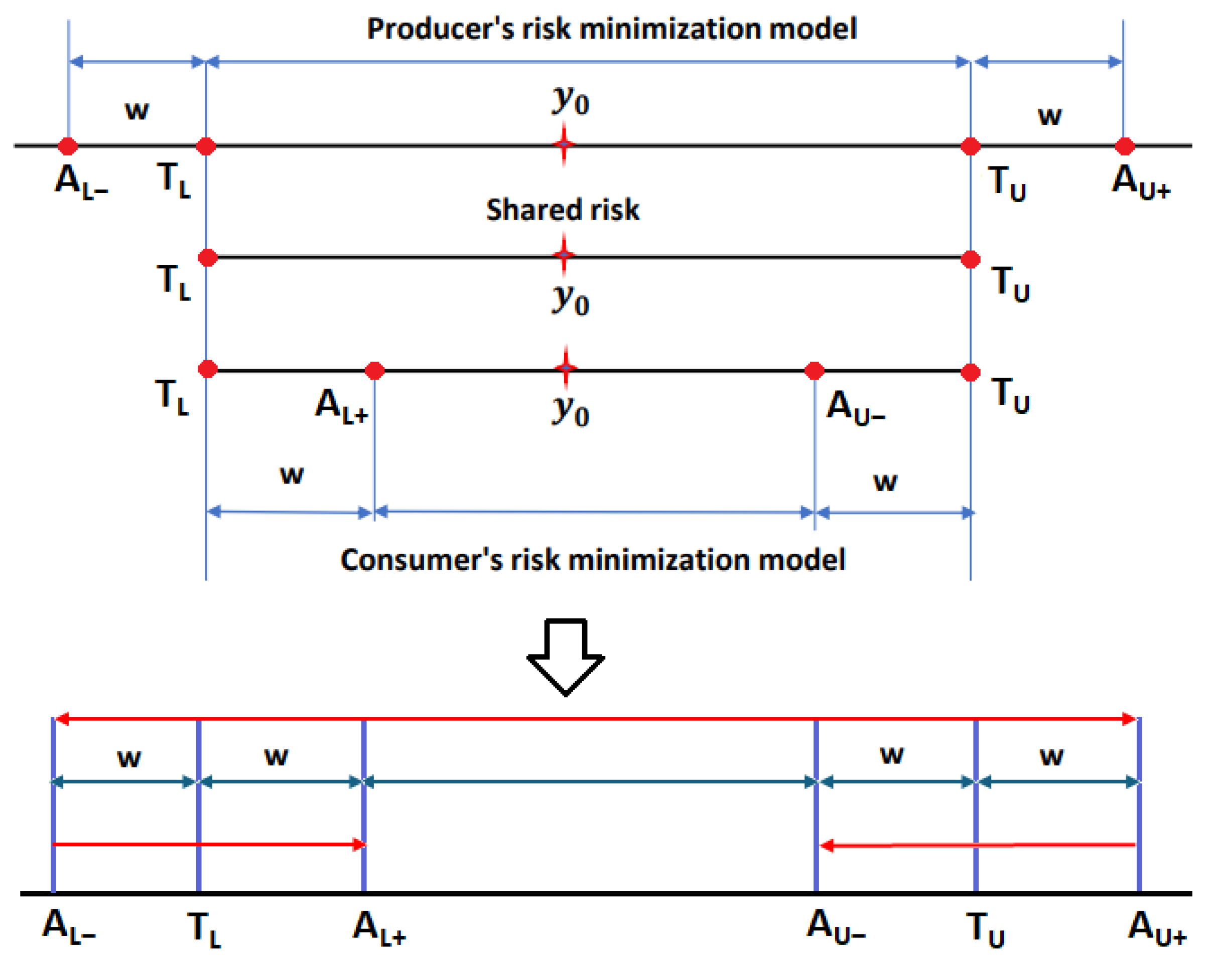
Figure 2.
Possible outcomes in a quality assessment procedure using a decision rule with a guard band and by including measurement uncertainty of future measurement: (a) true positive; (b) global producer's risk RP; (c) global consumer's risk RC; (d) true negative [50].
Figure 2.
Possible outcomes in a quality assessment procedure using a decision rule with a guard band and by including measurement uncertainty of future measurement: (a) true positive; (b) global producer's risk RP; (c) global consumer's risk RC; (d) true negative [50].
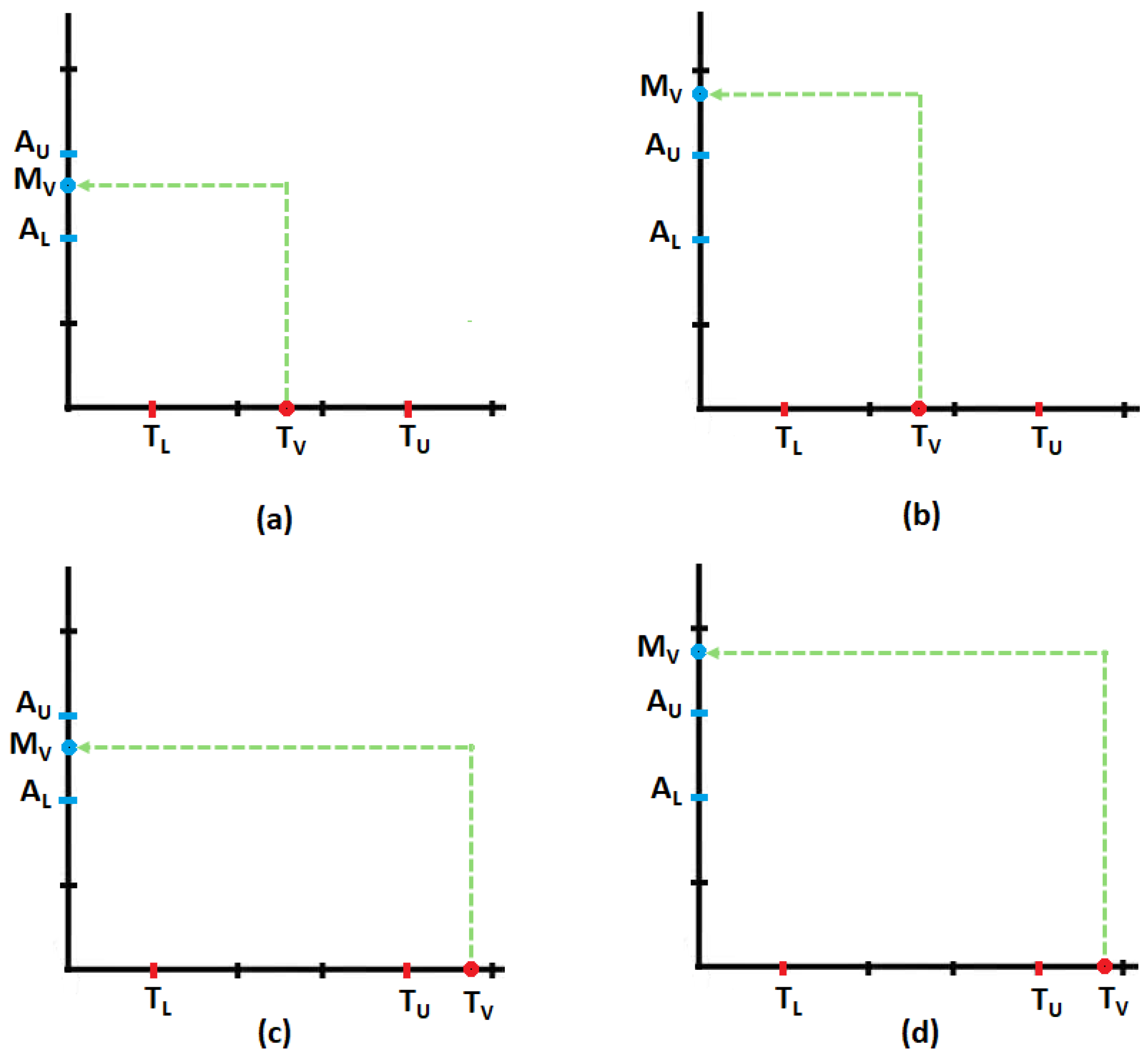
Figure 3.
Model geometry for spatial risk assessment: Case of minimization of global consumer's risk, .
Figure 3.
Model geometry for spatial risk assessment: Case of minimization of global consumer's risk, .
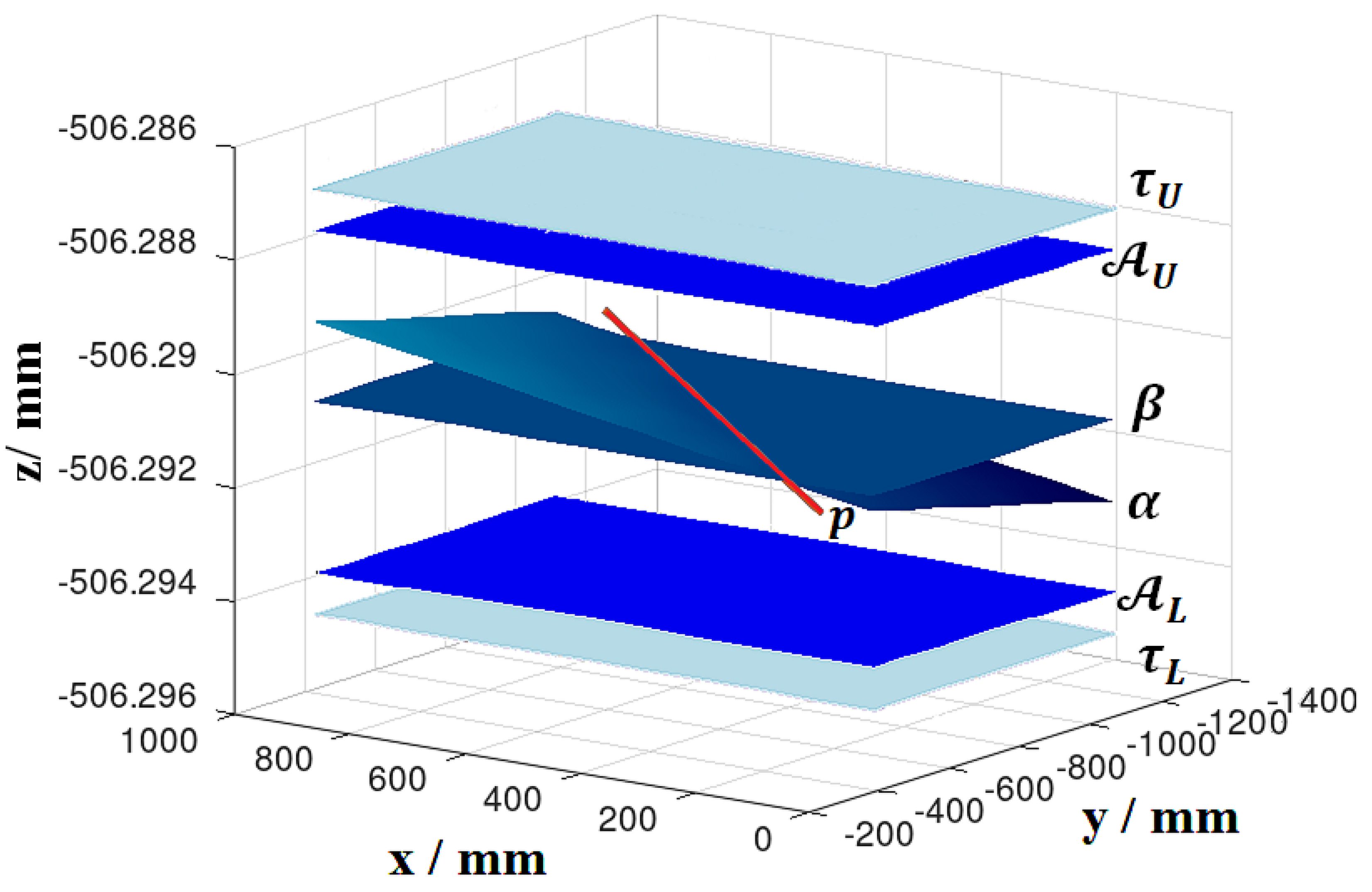
Figure 4.
(a) Global consumer's risk for the measured surface flatness values; (b) Minimum curves along guard band axis; (c) Global consumer's risk curves; (d) Global producer's risk curves.
Figure 4.
(a) Global consumer's risk for the measured surface flatness values; (b) Minimum curves along guard band axis; (c) Global consumer's risk curves; (d) Global producer's risk curves.
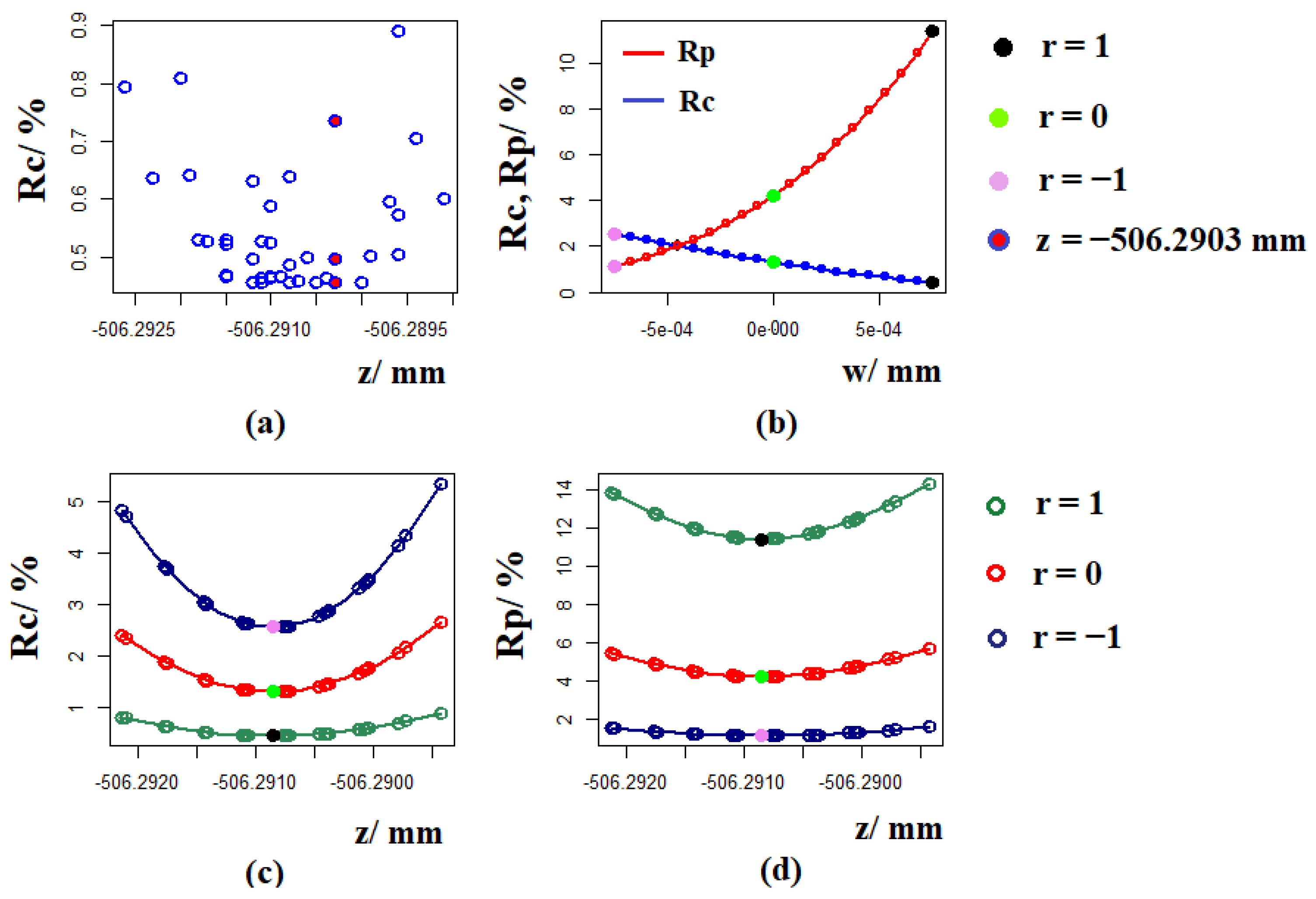
Figure 5.
(a) Risk surfaces; (b) Contour plots.
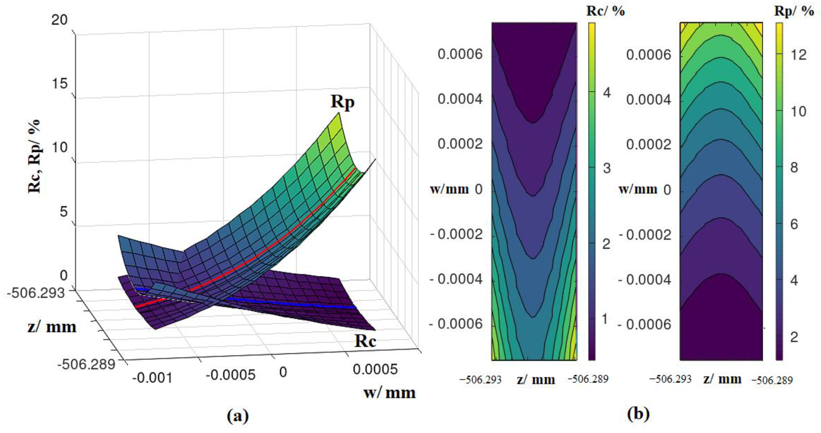
Figure 6.
Risk surfaces on domain for ; (a) Global consumer's risk; (b) Global producer's risk; (c) Contour plots.
Figure 6.
Risk surfaces on domain for ; (a) Global consumer's risk; (b) Global producer's risk; (c) Contour plots.
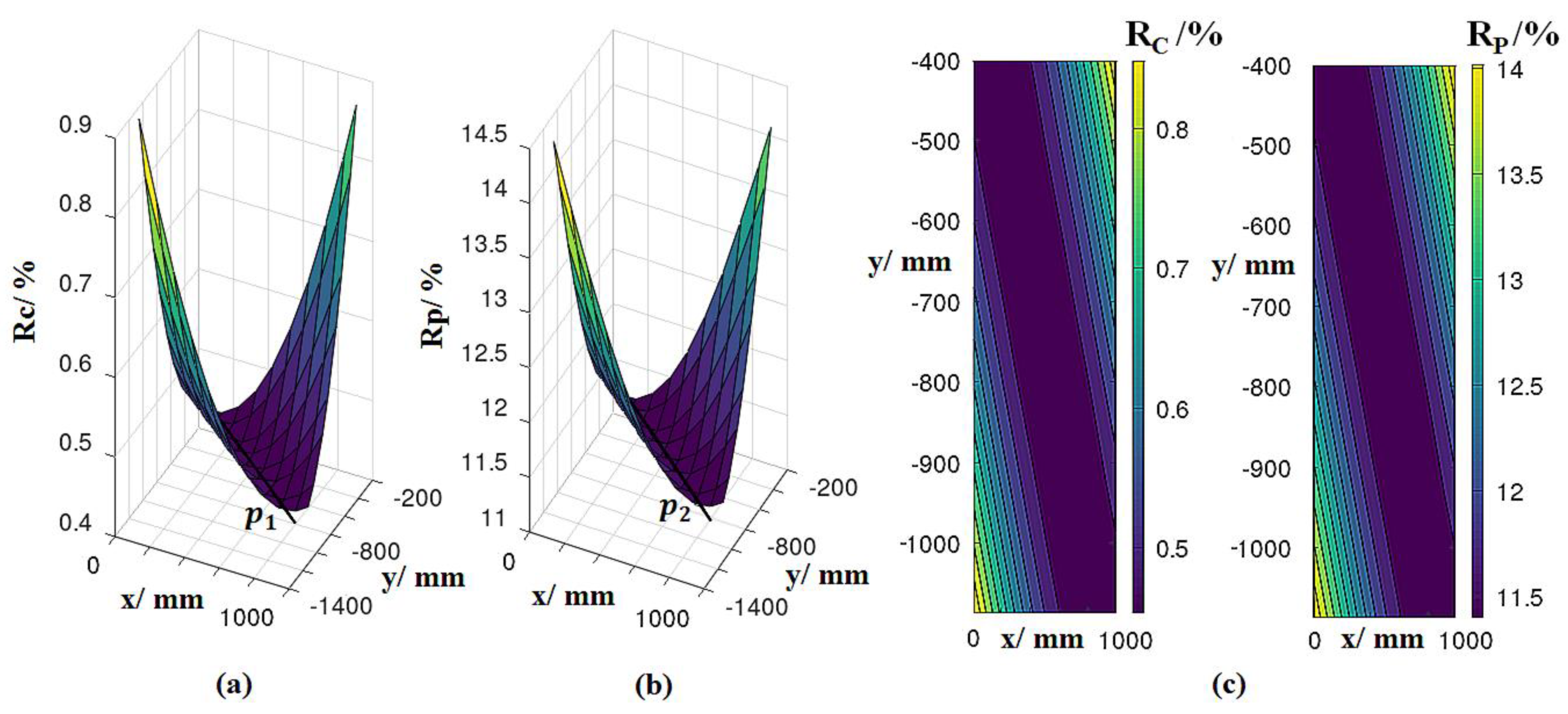
Figure 7.
Risk spaces: (a) Global consumer's risk; (b) Global producer's risk.
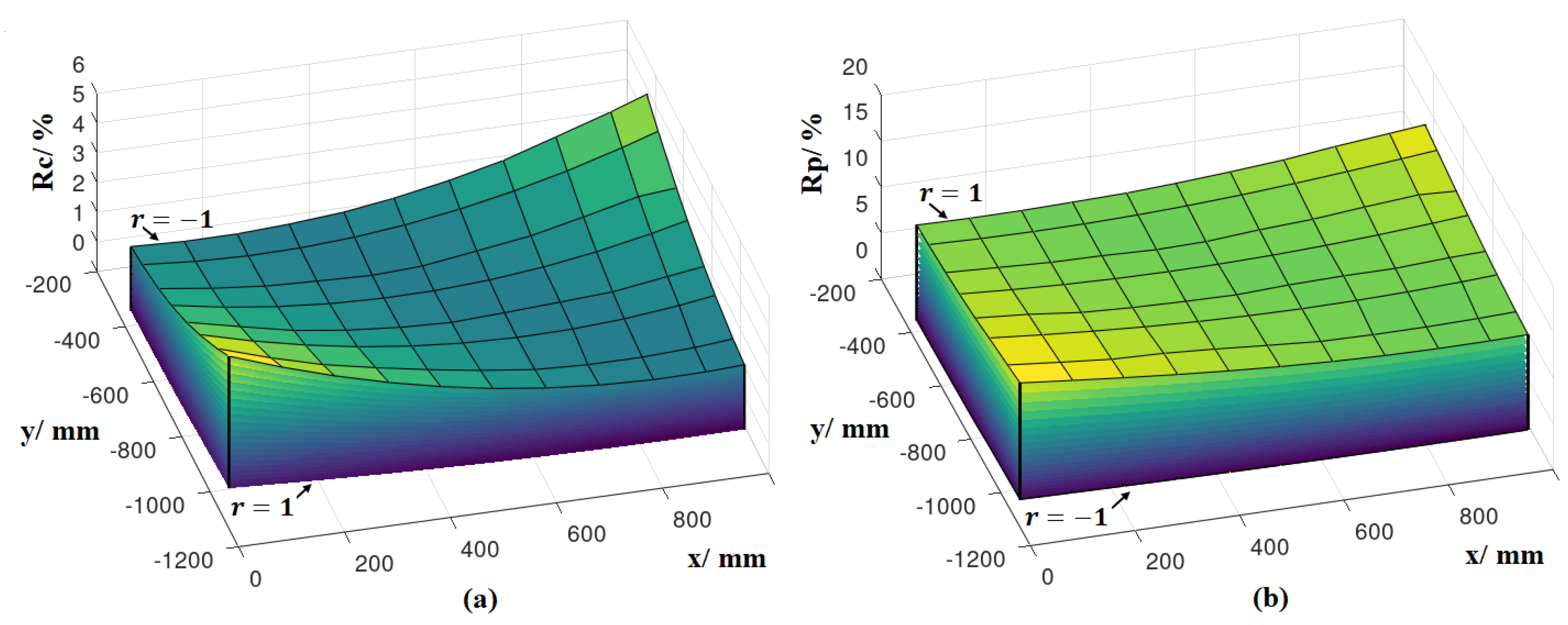
Figure 8.
Contour plots for different choices of reference planes, case of .
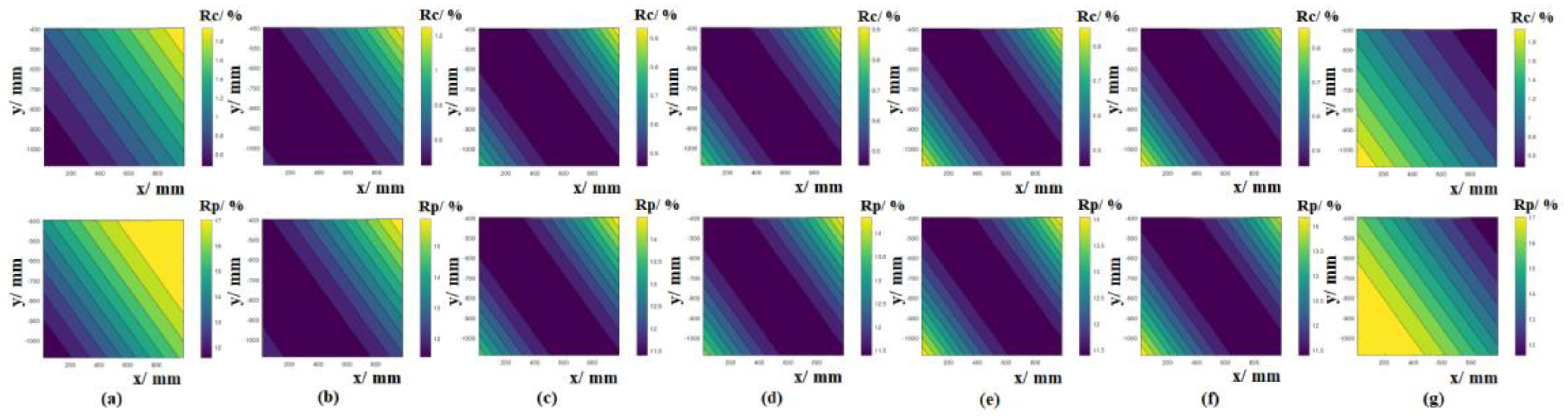
Figure 9.
Risk space for different values of measurement uncertainty .
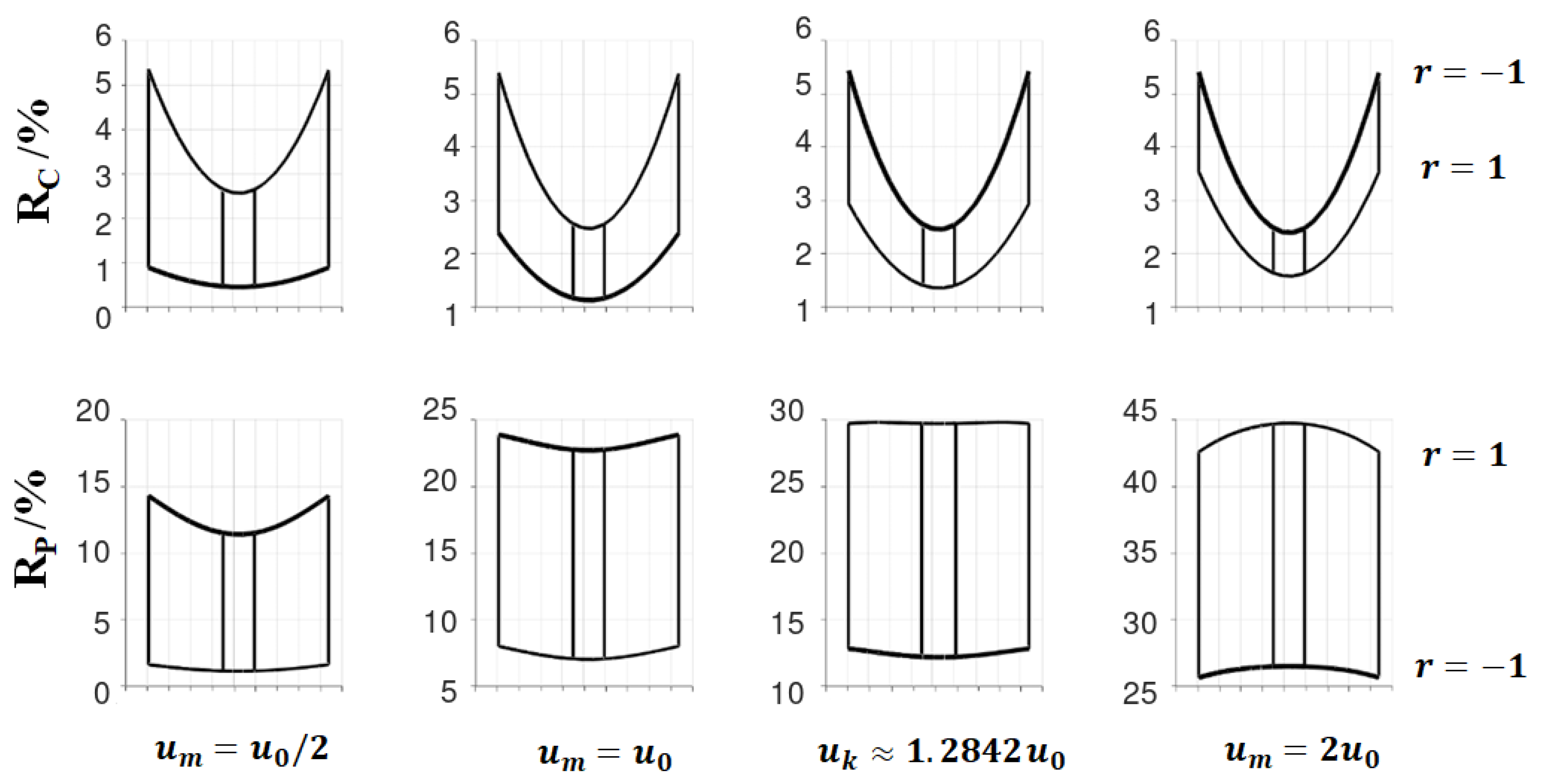
Figure 10.
Conformance probability on domain: (a) ; (b) .
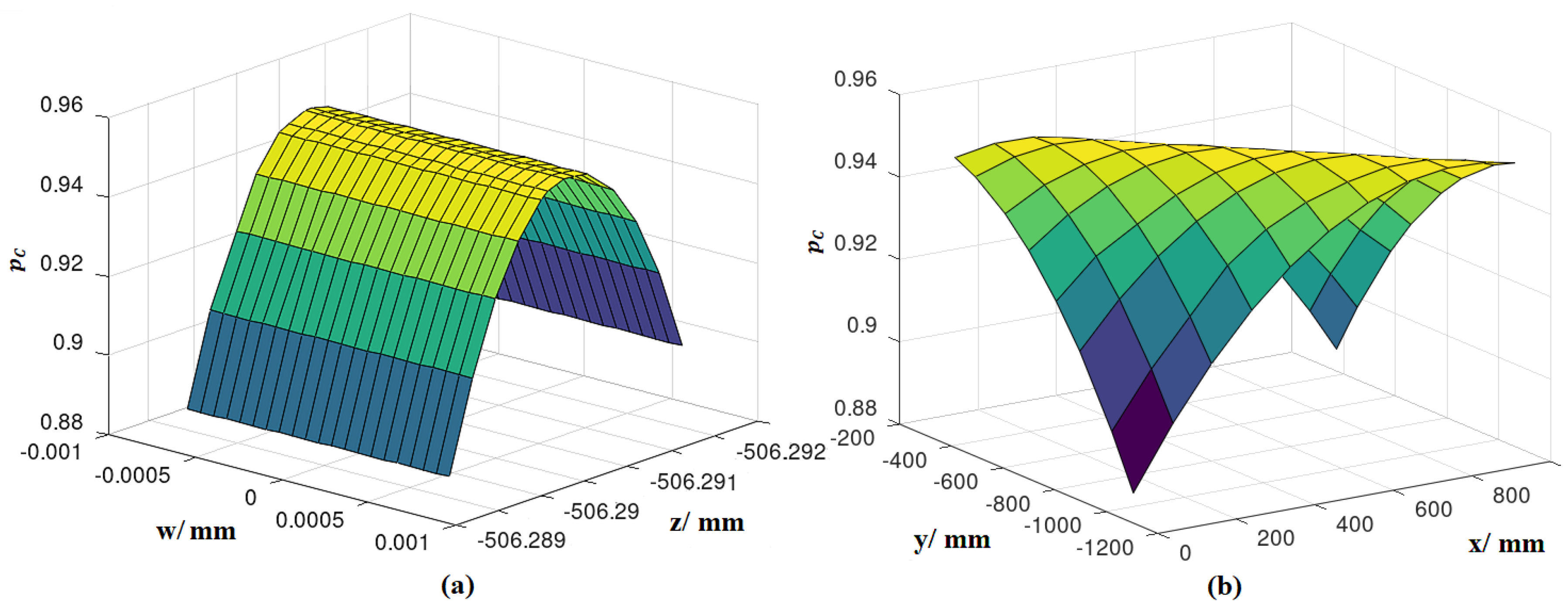
Figure 11.
(a) Plane division; (b) Confusion matrix.
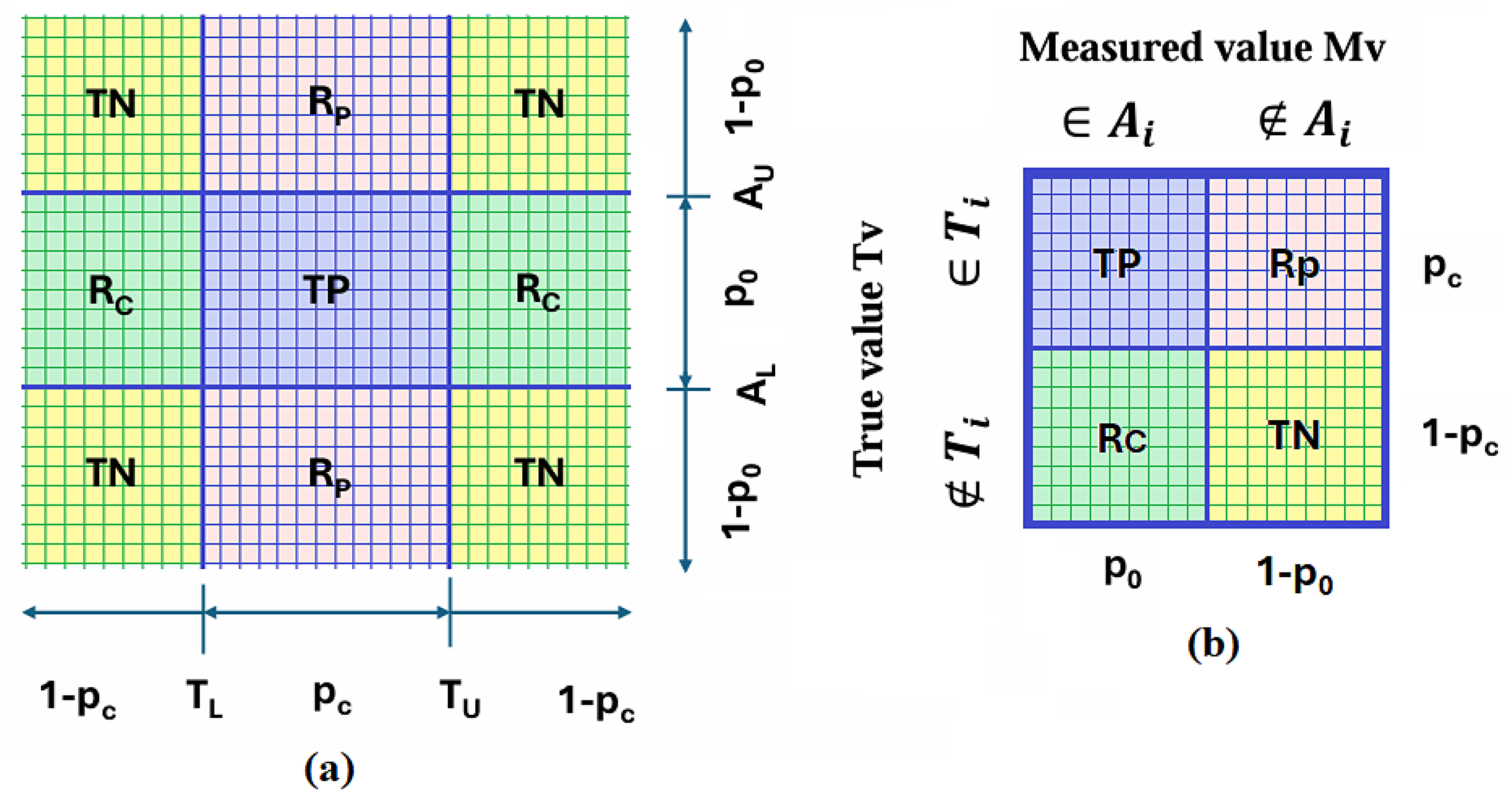
Figure 12.
(a) Probability space of frequent events; (b) Probability surfaces of frequent events
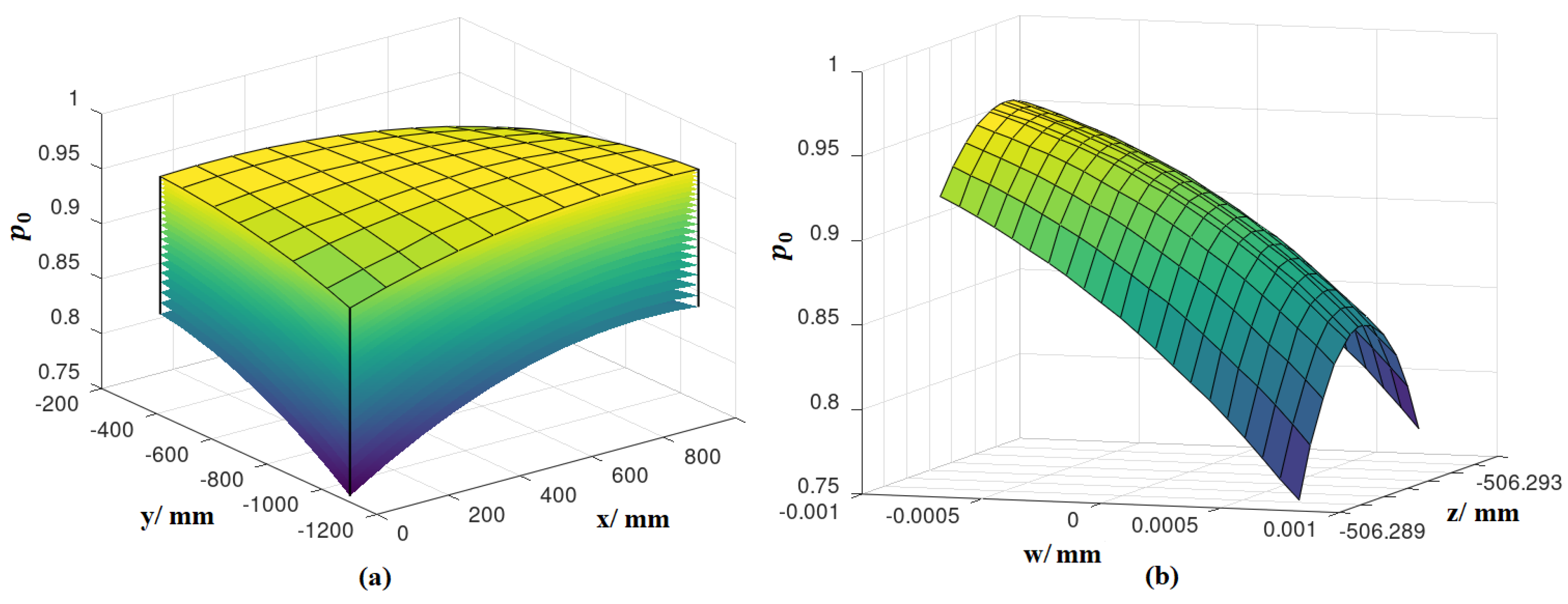
Figure 13.
Surfaces of metrics: (a) Matthews correlation coefficient; (b) Diagnostic odds ratio.
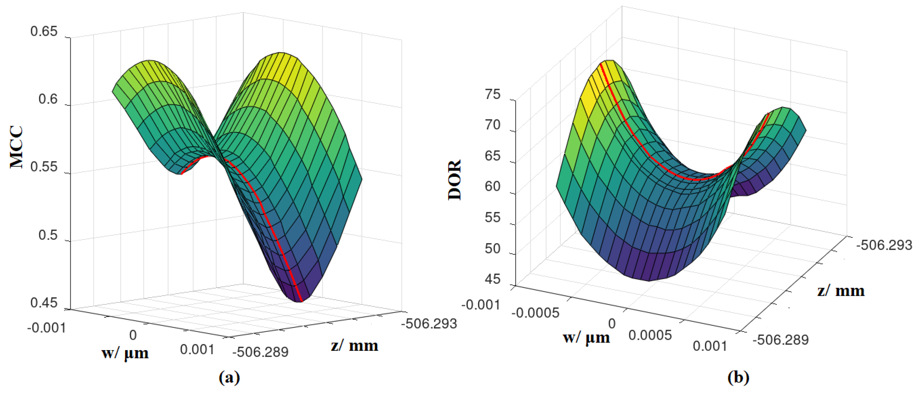
Figure 14.
Spaces of metrics: (a) MCC; (b) DOR; Projections: (c) MCC; (d) DOR.
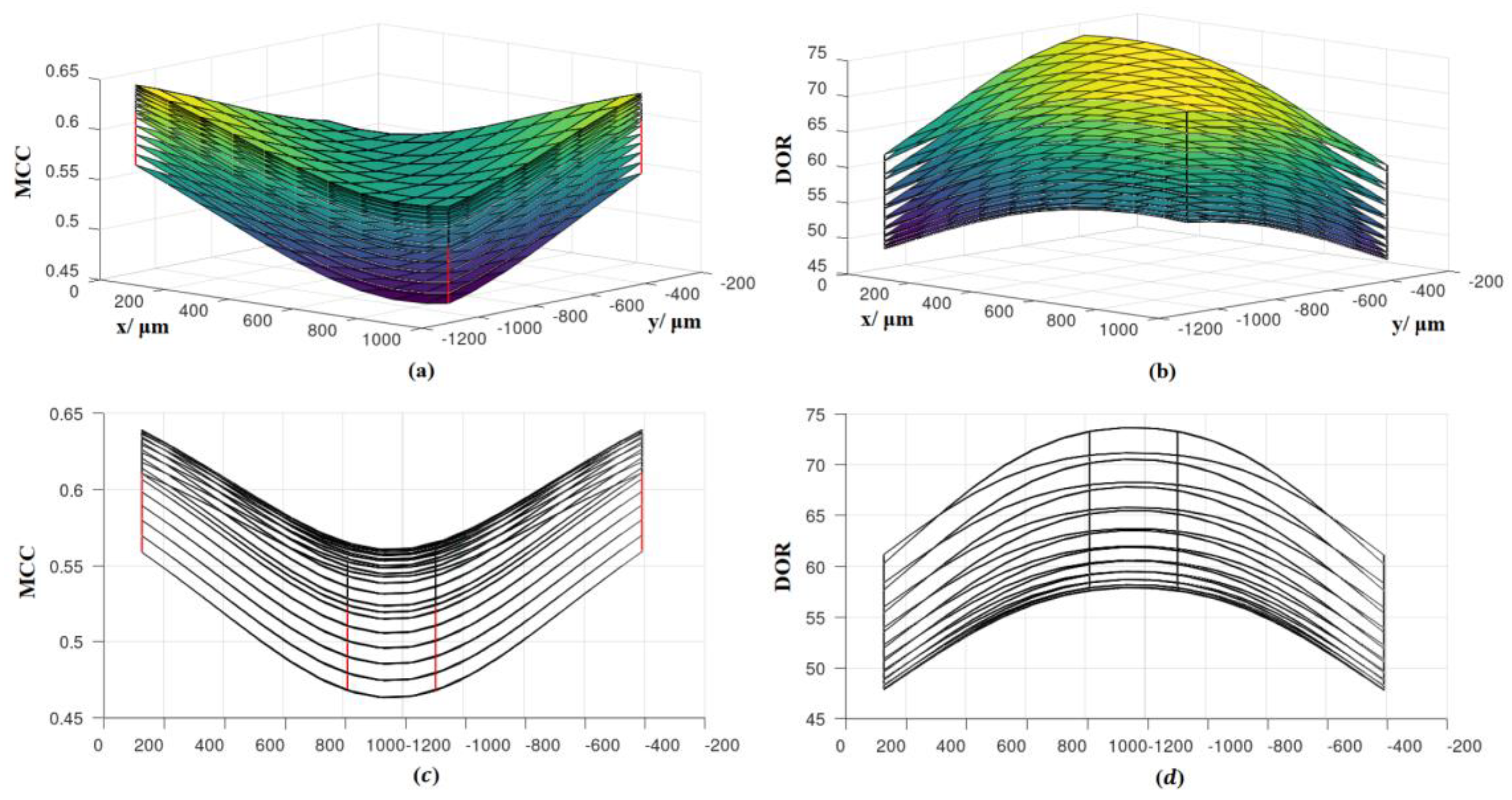

Table 1.
Injectivity intervals and guard band width for tested metrics.
| Labels | Metrics | mm | ||
| 1 | Accuracy | ↘* | 6.375 | 7.5 |
| 2 | F1 score | ↘ | 6.75 | 7.5 |
| 3 | BA | ↗ | 7.5 | 6.75 |
| 4 | G-mean | ↗ | 7.5 | 6.3 |
| 5 | BM | ↗ | 7.5 | 6.75 |
| 6L | kappa | ↗ | 7.5→3.75 | — |
| 6R | kappa | ↘ | 2.625 | 7.5 |
| 7L | MCC | ↗ | 7.5→3 | — |
| 7R | MCC | ↘ | 2.25 | 7.5 |
| 8L | DOR | ↘ | 7.5→0 | — |
| 8R | DOR | ↗ | — | 0.375→7.5 |
* ↘ Stacking layers in descending order. ↗ Stacking layers in ascending order.
Table 2.
Common injectivity intervals and the corresponding width of guard band.
| Intersection of intervals | Labels | mm | ||
| 1–5, 6L, 7L, 8L | 6.375→3.75 | — | ||
| 1–5, 6R, 7R, 8L | 2.25→0 | — | ||
| 1–5, 6R, 7R, 8R | — | 0.375→6 |
Disclaimer/Publisher’s Note: The statements, opinions and data contained in all publications are solely those of the individual author(s) and contributor(s) and not of MDPI and/or the editor(s). MDPI and/or the editor(s) disclaim responsibility for any injury to people or property resulting from any ideas, methods, instructions or products referred to in the content. |
© 2025 by the authors. Licensee MDPI, Basel, Switzerland. This article is an open access article distributed under the terms and conditions of the Creative Commons Attribution (CC BY) license (http://creativecommons.org/licenses/by/4.0/).
Copyright: This open access article is published under a Creative Commons CC BY 4.0 license, which permit the free download, distribution, and reuse, provided that the author and preprint are cited in any reuse.


