
Submitted:
31 October 2025
Posted:
03 November 2025
You are already at the latest version
Abstract
We present a new method for mapping of gas flares in the multiyear spatio-temporal database of the VIIRS Nightfire (VNF) nighttime infrared heat source detections from the three satellites, Suomi NPP, NOAA-20 and NOAA-21. The algorithm is composed of several steps: (i) 2D histogram binning of the high temperature (>1200 K) detection counts into 15 arcsec latitude-longitude grid, (ii) segmenting of the counts histogram into oil-field sized watershed features that serve as a guide where to search for the VNF detection clusters, (iii) super-resolution clustering the cloud of detections within each feature into a Dirichlet process variational Bayesian Gaussian mixture of compact clusters centered at the location of individual flare stacks, (iv) post-processing of the detected flares to avoid over-splitting and to find flare attraction contours with Voronoi/Apollonius geometry, (v) classification of the detection clusters into a pre-defined categories such as upstream, midstream, LNG, etc. with provenance from the earlier flare catalogs and multimodal LLM reasoning. The AI-assisted classifier uses reverse geocoding of the IR-emitter coordinates, high-definition daytime satellite imagery and time history profiles of the detections inside attraction contours to hint the expert with a probable category of the emitter together with the short summary of reasoning. Compared to the annual catalogs used for the country-level estimates of flared gas volume, the new algorithm is robust to atmospheric glow from large flares (higher selectivity) results in twice the number of the active flares (higher sensitivity), located with subpixels precision ~50 m and separable within ~400-700 m. For the well-defined class of downstream flares at export LNG locations the catalog demonstrates near-complete detectability.
Keywords:
gas flaring
; multiyear flare catalog
; VIIRS
; upstream oil and gas
; LNG
; country-level totals
; flare stack localization
; super-resolution
; Dirichlet-process Gaussian mixture
; watershed superpixels
1. Introduction
Remote sensing of gas flaring from space began with coarse nighttime imaging. The DMSP-OLS (Defense Meteorological Satellite Program Operational Linescan System) was the first sensor to map global flare activity at night, though it lacked spectral detail and radiometric calibration, limiting quantitative use [1]. Calibrated mid-infrared (3.9 µm) MODIS data from NASA’s Terra and Aqua platforms enabled more systematic detection of heat sources, but infrequent revisit time and absence of the most nighttime flare-sensitive short-wave infrared (SWIR) bands constrained global monitoring [2,3].
The launch of the Visible Infrared Imaging Radiometer Suite (VIIRS) on Suomi NPP and NOAA-20/21 satellites provided a breakthrough for global detection and monitoring of industrial infrared emitters [4]. VIIRS has finer spatial resolution (750 m at nadir), a broad dynamic range, in-flight radiometric calibration and nighttime multispectral imaging including SWIR (M10, 1.6 µm and later M12, 2.2 µm). Building on these features, in 2012, the Earth Observation Group (EOG) developed and began producing a multispectral nightly global infrared emitter data product known as VIIRS Nightfire (VNF) [5]. The algorithm detects sub-pixel combustion sources by fitting Planck curves to multispectral radiances, retrieving source temperature, size, and radiant heat. This made it possible to estimate flared gas volumes [6] and build long-term flare catalogs.
The VNF algorithm exploits the detection of sub-pixel infrared emitters in four daytime VIIRS channels that continue to collect at night (Figure 1). This includes two spectral bands in the near infrared (M7 and M8) and two in the shortwave infrared (M10 and M11). With solar illumination absent, these daytime channels record the sensor noise floor, punctuated by clusters of high radiance levels arising from subpixel infrared emitters, such as biomass burning, natural gas flaring, industrial waste heat, and volcanos. In such cases, the detected NIR and SWIR radiances can be fully attributed to the Earth surface IR emitters. This makes it possible to calculate the IR emitter’s temperature, source area, and radiant heat using physical laws [5].
Daytime detection of gas flares using medium-resolution sensors Sentinel-2 MSI (MultiSpectral Instrument) and Landsat-8/9 OLI (Operational Land Imager) was developed by several groups, enabling global and regional inventories that complement night-time VIIRS products and better resolve heat sources with ~30 m pixel footprint. Recent efforts span global catalogues and algorithm advances (e.g., DAFI, Daytime Approach for gas Flaring Investigation algorithm and its multi-sensor extensions [7,8]) as well as regional time-series applications [9], together demonstrating flare mapping from daytime optical/SWIR data. In practice, Sentinel/Landsat daytime products provide finer spatial discrimination (useful for source separation), while VIIRS night-time VNF provides higher thermal contrast and more reliable radiometry for flux-oriented retrievals. Furthermore, the satellites employed exhibit less frequent revisit times compared to the VIIRS satellites, which provide 3–5 overpasses per night.
From the beginning, we designed VNF to build long-term records of thermal and activity levels across as many industrial sites as possible. To achieve this objective, we developed methods to catalog and systematically organize the temporal records of Earth-surface infrared emitters. Each catalog is based on compositing of a year or more of nightly global VNF detections into 15 arc second summary grids, recording the average temperature, number of cloud-free detections, and percent frequency of cloud-free detections. VNF pixels entering 15 arc second summary grids are required to have temperatures and be a local maximum in the M10 SWIR band. In most catalogs a temperature threshold of 1200 K is set to focus on natural gas flares. Biomass burning is filtered out based on its low temperature and low percent frequency of detection. The remaining 15 arc second grid cells are analyzed to derive IR emitters with identification numbers, centroid locations, bounding vectors, and emitter type labels. The catalog bounding vectors are then used to create temporal profiles, suitable for analysis of flared gas volumes and history of individual industrial sites [10]. The rationale for single year flare catalogs is that each year there are new flares, especially in the USA, where oil and gas production is dominated by “fracking” techniques applied to deep shale formations.
The downside to the single-year-flare catalogs is that in each year, the strategy has been to set a threshold that splits the difference between thorough detection of small infrequent flares and the erroneous labeling of glow patches as flares. Working solely with the 15 arc second summary grids there is always a tension between inclusion of small intermittent flares and the glow surrounding closely spaced clusters of large flares. Filtering the 15 arc second summary grids to include more of the small flares results in larger number of false flares arising from atmospheric scatter, which we term glow. Figure 2 shows examples of this under-detection of small infrequent flares and false detections in the glow around large flares. This problem is present in all of the VNF IR emitter catalogs from 2012 through 2024 [11]. Additionally, new identification numbers are assigned to all identified IR emitters, new bounding vectors are established, and lower-temperature industrial emitters are underrepresented.
Using multiyear VNF time series, Liu et al. in 2018 proposed an object-oriented algorithm that groups nightly thermal anomalies into persistent “heat source objects” and classifies them with spatio-temporal and thermal fingerprints covering multiple industrial heat sources (not just flares). Importantly, they also produced a rasterized VNF detection map (gridded accumulation of detections), analogous to annual VNF catalogs, to derive persistence/intensity features for object formation and labeling [12].
In 2020, EOG developed the concept for an all-temperature multiyear catalog that would be filtered to remove biomass burning, include both flares and industrial sites, assign permanent identification numbers, and a single bounding vector [13]. This multiyear catalog was produced for 2012 through 2022 and is known as MYC22 (multiyear catalog 2022). With permanent identification numbers and bounding vectors valid for all years, MYC22 enabled the development of nightly temporal profiles extending from March 2012 to the present. The MYC22 catalog continues in use to this day, with temporal profiles updated on a weekly basis. MYC22 has a wide range of emitter types, shown in Table 1.
The development of the super-resolution method for distinguishing actual IR emitters from glow occurred midway through the MYC22 production. The MYC22 summary grids are filtered based on the precent frequency of VNF detection to remove both biomass burning and high temperature glow surrounding large flares. The percent frequency threshold is 2% from 400 to 1300 K and drops to 1% from 1300 to 2500 K (Figure 3). These thresholds are set based on samples extracted from dense clusters of biomass burning in Bolivia and Cambodia to set the low temperature noise floor. The high temperature noise floor is set based on clusters of flare glow grid cells extracted in the Basra region of Iraq. The 15 arc second percent frequency of detection thresholds are set to remove most of the biomass burning and flare glow, but enough remains to requiring a second filtering step to clean up the catalog. The challenge of this secondary filtering for MYC22 led to the development of the super-resolution method for distinguishing between real surface emitters and glow.
Super-resolution refers to the identification of surface emitters based on clustering of the VNF pixel center latitudes and longitudes. The VIIRS pixel footprints land randomly and never exactly repeat. While the pixel footprint center location is known, the precise location of the emitter could be anywhere inside the pixel footprint. It is even possible for the radiant energy from a single emitter to be split between two or more VNF pixels. The super-resolution method skips over the blurring effect associated with the binning of VNF detections into 15 arc second grid cells. The result is a precise geospatial mapping of the cumulative footprint of VNF detections associated with surface emitters. The MYC22 is flawed because the 15 arc second filtering drops many small infrequent IR emitters.
This paper describes the development of a new flare catalog that uses a 15 arc second detection tally grid only as a guide to identify candidate basin or oil-field size regions which possibly contain gas flares. The super-resolution analysis then screens out the glow, preserving smaller, infrequent flares missing from the previous catalogs.
2. Materials and Methods
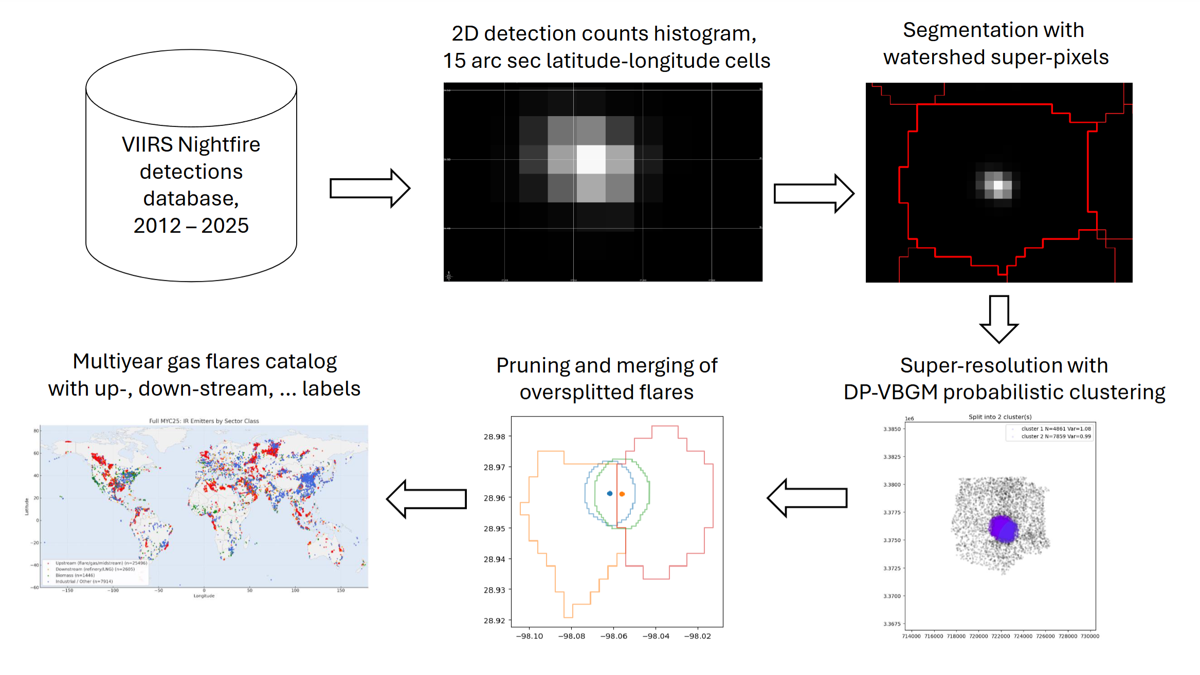
We present a multi-step algorithm for building a high-resolution catalog of flaring sites from VIIRS Nightfire (VNF) detections spanning 2012–2025. The algorithm integrates 2D histogram rasterization of VNF detection counts, watershed segmentation, probabilistic clustering, post-processing with pruning and merging, and finally AI-assisted attribution (industrial type and operator). Each step addresses a specific limitation of raw satellite detections, transforming irregular per-pixel detections in multispectral imagery into a validated, consistent catalog of unique, persistently flaring point sources (Figure 4). This approach differs substantially from the flare-survey methodology [10] used since 2015 in the World Bank’s annual flaring reports [11].
Step 1. Rasterization of VNF Detections
Raw VNF detections, stored as point geometries in PostgreSQL spatio-temporal database with attributes such as source area, temperature, and radiative heat, are aggregated onto a regular latitude–longitude grid to create detection-count rasters. This converts irregular detection points into a continuous surface, providing a map of the geographical distribution and temporal persistence of flaring activity and a basis for subsequent algorithmic segmentation. We use all VNF version 3.0 detections from the three VIIRS platforms (Suomi NPP, NOAA-20, and NOAA-21) spanning March 2012 to March 2025, subject to two filters: (i) VNF-estimated source temperature T > 1200 K and (ii) the corresponding VIIRS M10 band (1.6 µm) pixel is a local maximum. These constraints suppress atmospheric glow around large flares and exclude cooler industrial sources and most biomass burning.
The global detection count map is then split into latitude–longitude tiles of size 15° to accelerate data processing with parallel computer cluster, each tile representing a 2D histogram on a 15-arcsecond grid (≈ the VIIRS M-band pixel footprint), where cell values equal the number of detections. This rasterization yields a continuous surface for locating spatial clusters while smoothing irregular sampling caused by orbital coverage and cloud obscuration. Figure 5 illustrates the result of VNF detection counts rasterization for a region with multiple flares in Basra, Iraq.
Step 2. Watershed Segmentation of Candidate Features
The goal of this step is to partition the rasterized VNF detection count map into manageable superpixels [14] to delineate candidate regions where flares are likely to occur, so that the next, super-resolution clustering step remains tractable. Because that clustering is both time- and memory-intensive, each superpixel must be small enough to run on a single compute node; conversely, superpixels that are too small risk splitting a compact flare cluster at their boundaries. As a rule of thumb, we target fewer than ~30 flares per superpixel.
Operationally, we apply watershed segmentation [15,16] to the detection-count raster: local density peaks are identified as markers (watershed seeds), and flooding is performed on the inverted raster so that each basin corresponds to a dense detection region (hydrological analogy). To reduce over-segmentation, we apply morphological post-processing (expansion and smoothing) before polygonizing the resulting superpixels (Figure 6). Hereafter, we refer to these watershed-derived superpixels as “waterpixels,” following the usage and formulation of Machairas et al. [16].
Step 3. Super-Resolution Clustering of Detections
For localized (point-type) persistent IR emitters, VNF detections typically form dense rotated-square (diamond) clusters centered on the source. The characteristic size of each cluster is approximately the VIIRS M-band pixel footprint (≈ 1.6 km), and its orientation is set by the satellite ground track/scan geometry. The goal of super-resolution clustering is to unmix these dense detection clouds within each waterepixel into a set of (potentially overlapping) square-shaped clusters, each centered on the location of a real flare.
Within each waterpixel, we retrieve from the database the relevant VNF v3.0 detections and project their pixel centers to a local UTM frame for metric accuracy. The database filter at this step is more permissive than in Step 1: we impose no temperature threshold, but require that the corresponding pixel in at least one VIIRS M-band (M10: 1.6 µm, M11: 2.2 µm, or M13: 4.1 µm) be a local maximum and pass a white top-hat test. The white top-hat transform in mathematical morphology emphasizes compact bright peaks while suppressing broad background glow:
where f is the band image, se is a disk-shaped structuring element tuned to the VIIRS M-band footprint, ⊖ is erosion, and ⊕ is dilation [17]. A positive top-hat response together with the local-maximum condition effectively suppresses atmospheric glow around large flares while retaining true, point-like emitters.
Twhite(f) = f – (f ∘ se), (f ∘ se) = (f ⊖ se) ⊕ se,
A Dirichlet-process Variational Bayesian Gaussian Mixture (DP-VBGM) [18,19] is then fitted to the data, using spherical covariance models. This clustering assigns detections to sub-clusters, each representing a probable distinct flare stack. The probabilistic framework ensures that the number of clusters is inferred from the data rather than fixed, enabling adaptive resolution in dense industrial regions.
Formally, we fit a Dirichlet-process variational Bayesian Gaussian mixture (DP-VBGM) to detections in a local UTM frame, independently within each waterpixel. The per-waterpixel fits run as loosely coupled, communication-free parallel tasks on the compute. The data likelihood is modeled as a truncated mixture of isotropic (circular) Gaussians,
with a Dirichlet-process prior that shrinks many weights {πk} toward zero. Variational Bayes infers the posterior “responsibilities”
and we take hard assignments via . This way, the model lets the data determine the effective number of clusters, avoiding manual tuning and reducing over- and under-splitting.
For each cluster of VNF detections modeled as an isotropic 2D Gaussian in the local UTM plane we define a spatial compactness scale
where σ is the per-axis distance standard deviation and the distance root mean square is a statistical concept used to measure the dispersion of a set of projectile impacts in ballistics. Then, for an isotropic Gaussian, the fraction of points within radius r is P(r)=1−exp (−r2/(2σ2)); at radius this circle encloses of the VNF detections. Thus, V is a convenient, interpretable proxy for cluster compactness, and Varmax provides a consistent acceptance threshold across sites.
Figure 7 illustrates how the super-resolution step separates multiple, closely spaced emitters inside a single waterpixel. The left panel is a detection density surface (≈100 m grid, tenfold more detailed than the detection count raster in the Step 2). A compact, rotated-square hotspot is evident, consistent with a point-source flare viewed in the VIIRS scan geometry; the surrounding low-intensity halo reflects occasional geolocation jitter and multiple atmosphere scattering effects.
The right panel shows all VNF detection centers (gray) projected into a local UTM frame and partitioned by a Dirichlet-process Gaussian mixture into four subclusters (colored). For each cluster the legend lists N (detections assigned) and Var (the covariance-derived spatial scale, in km). Here, Var values (~0.8–1.05 km) are well within the acceptance threshold Varmax ≈1.6 km, indicating compact, well-resolved sources. The cluster compactness threshold was empirically set to exclude most of the false-detected clusters with no visible flare inside in the corresponding high-resolution daytime (HRD) image. Sure enough, empirically estimated value comes close to the maximum VIIRS M-band pixel footprint.
Cluster boundaries (we call them “bubble vectors”) ensure each VNF detection (pixel) is unambiguously assigned to a single flare, preventing overlap and double-counting within dense flare groups. With unique ownership defined, we can reliably aggregate radiance and temperature from instantaneous satellite detections and build per-flare flowrate histories, while at the same time the boundaries coincide with the most-likely decision surfaces under the DP-VBGM: each pixel x with VNF detection is assigned to the flare k with the highest posterior probability p(k ∣ x), so decision surfaces occur where p(k ∣ x) = p(ℓ ∣ x) between overlapping 2D Gaussian PDFs for clusters k and ℓ. With isotropic (circular) covariances and equal priors, these weighted nearest-centroid boundaries reduce to Voronoi/Apollonius partitions [20,21,22].
Let the flare PDF centroids be {μk} with compactness scale sk (e.g., covariance-derived Var of the DP-VBGM unmixed clusters). We define a weighted discriminant distance
and assign each location x to the site with minimal Dk(x). The pairwise boundary between sites k and ℓ is the locus
which is the classical Apollonius problem: a boundary that is a circle. Thus, equal scales yield the usual Voronoi cells; unequal scales produce Apollonius (weighted Voronoi) cells that shrink around tighter, better-constrained clusters.
Final flare attraction contours (we call them “bubble vectors”) are taken as the weighted Voronoi/Apollonius cells, intersected with an elliptical confidence region
This yields non-overlapping, size-aware contours that honor both geometric proximity and statistical separability of distinct flare clusters.
In practice, we do not need the closed-form Voronoi/Apollonius solution (even though it exists) because GIS and database workflows require polygons. Instead, we work in a local UTM grid and compute an approximate, GIS-ready partition numerically: lay down a fine raster (≈100 m cells), evaluate for each cell center x the discriminant distance Dk(x), assign the label arg maxk Dk(x), (max posterior responsibility), and polygonize the labeled raster into vector footprints. The result closely matches the theoretical Voronoi/Apollonius boundaries, while avoiding arc-to-polygon conversion.
Figure 8 shows the resulting polygon outlines of the inferred footprints and the centroids provide point estimates of individual flare stack locations. Partial polygon overlap is expected where stacks are very close together or when occasional off-nadir views and clouds broaden the point cloud. Overall, the Figure 7 and Figure 8 demonstrate that the method can unmix multiple emitters within subpixel distances between each other, producing site-level centroids and footprints suitable for subsequent cleaning (Step 4) and provenance-aware AI classification (Step 5).
Step 4. Cleaning and Post-Processing
Post-processing flare catalog cleanup is needed to correct two types of errors shown in Figure 9: (i) duplicate flare detection clusters which eventually get split at the boundary of the adjacent waterpixels and (ii) occasional oversplitting of the dense flare stacks or elongated industrial infrastructure into clusters which are too close to be resolved in satellite images.
To de-duplicate the flares split at tile/waterpixel edges, we test polygon overlap and centroid proximity and retain the strongest candidate, defined as the one with greater evidential support (more detections/unique dates) and higher compactness (smaller Var).
To merge back the over-split flares, we run DBSCAN [19] on cluster centroids using a geodesic metric (Haversine) with a merge radius of VIIRS M-band footprint ε = 600 m. DBSCAN naturally groups any number of over-splitted clusters. For each DBSCAN group of two or more VNF detection clusters, instead of choosing a single survivor, we compute a weighted-average centroid in a local UTM frame,
where Ni is the number of detections assigned to cluster i. This yields a representative location proportional to evidential support. After de-duplication, we re-draw the cluster contours using Voronoi/Apollonius construction informed by 2D discriminant analysis seeded by the cleaned centroids (flare coordinates).
Figure 10 shows the result of cleaning for the same facility as in Figure 4. Prior to cleaning, it had two overlapping polygons from near-duplicate detection clusters. Cleaning has merged the near-duplicates using spatial proximity with DBSCAN, then re-contoured the footprints with Voronoi cells. Compared against HRD image, the final centroids coincide with visible flare stacks to better than 100 m, confirming positional accuracy.
Step 5. Provenance and AI-Assisted Labeling of Newly Detected Sites
To improve the interpretability of the flaring site catalog, the algorithm integrates provenance knowledge and AI-driven labeling in its final step. Newly detected sites are first cross-matched against earlier catalogs (e.g., MYC22, Annual 2024) and authoritative external datasets to transfer existing flare type classifications where possible.
For sites without prior records, reverse geocoding supplies essential geographic context—country, administrative units, and nearby infrastructure by translating site coordinates into human-readable place attributes (e.g., postal addresses, business names) [23]. A multimodal AI assistant then combines this geocoding context with daytime HDR satellite image centered at the site and with VNF-derived tabular features (e.g., temperature, persistence, radiance) to propose a site classification, while producing a brief explainable rationale to make the decision auditable. The assistant assigns each site to a fixed set of labels (upstream flare, downstream flare, industrial site, biomass burning, or unknown) and returns the most-likely label together with a short justification for decision. Results are integrated into an interactive map (Figure 11): clicking on a pushpin opens a panel with the AI-suggested label, any provenance matches to prior catalogs, and supporting evidence. This approach preserves continuity with historical datasets via provenance linking while filling gaps through automated, explainable and verifiable classification.
3. Results
The multiyear flare catalog (MYC25) identified a total of 25,045 upstream flares (from both oil and gas fields) active between March 2012 and March 2025, a significant increase compared to the 10,688 upstream flares identified in the annual flare catalog used in the World Bank 2024 Flaring Report. The global inventory map of MYC25 is shown in Figure 12.
The pie chart in Figure 13 provides a MYC25 breakdown by type (upstream, midstream, and downstream), offering insights into the distribution of high temperature IR emitters. Upstream operations dominate the total oil and gas flaring activities, followed by midstream and downstream processes. High temperature IR emitters, which are not associated with the oil and gas flaring, such as chemical plants or landfills, are assigned to the generic “industrial” class.
3.1. Sensitivity and selectivity
The MYC25 combines definitive historical VNF detections database from three VIIRS satellites with recent near-real-time (NRT) preliminary dataset, segmented into waterpixels to be tractable for super-resolution clustering. The Dirichlet-process prior adapts the number of dense clusters with predefined 2D Gaussian detections cluster shape to the data, enabling finer resolution in dense complexes and removal of less compact detections from wildfires and atmospheric glow. In practice, this increases true-positive recovery of real flares (higher sensitivity) that annual windows miss due to limited dwell time (e.g. Colorado, Figure 14) while reducing false positives (higher selectivity) such as glow-induced artifacts around the largest flare stacks (e.g., Venezuela, Figure 15).
For each year evaluated, the MYC25 workflow reports about twice as many active flares as the corresponding annual snapshot catalogs. The by-country comparison in Figure 16 shows that in 2024 the MYC25 enumerates more active emitters in as the Annual 2024 catalog, with the largest count increases in the United States (+4857; 8402 vs 3545), China (+561; 1163 vs 602), Canada (+540; 1049 vs 509), and the Russian Federation (+488; 1946 vs 1458. By contrast, the Venezuela flare count is lower in MYC25 (−27; 176 vs 203) due to stronger glow suppression.
3.2. Duty cycle and number of detections
By integrating detections across 2012–2025 from Suomi-NPP, NOAA-20, and NOAA-21 satellites, the MYC25 captures infrequent or intermittent flares that annual catalogs systematically miss. Intermittency (how often a flare is detected when the satellites actually have a chance to see it over a chosen period e.g., a year) may indicate that a flare has become unlit and possibly venting unburnt methane, while continuity of flare detections over time is indicative that flaring is probably routine, that is a key parameter when assessing potential for utilization of the flared gas.
To compare the number of detections per flare and their duty cycles (the fraction of observing opportunities, in our case valid satellite overpasses, during which the flare was detected) between MYC25 and Annual 2024, we selected from both catalogs upstream flares detected at least once in 2024 and present the distributions in Figure 17 with summary metrics in Table 2. The distribution of the number of detections in 2024 is shifted lower in MYC25, with a median of 13 compared to 31 in Annual-2024; very low detection counts are rare in both catalogs. Similarly, the duty cycle (the fraction of observing opportunities with detections) is systematically lower in MYC25: the median duty cycle is 0.05 in MYC25 versus 0.13 in Annual 2024. These population-level contrasts are consistent with MYC25’s finer emitter delineation and inclusion of more intermittent flares, which collectively lower duty cycle and number of detections per flare compared to annual catalogs.
3.3. Localization precision and minimum separable distance.
The MYC25 flare catalog demonstrates a high degree of spatial consistency when compared with the legacy MYC22 IR emitters catalog. A nearest neighbor cross-match between the catalogs, using a conservative 300 m association threshold, reveals small positional offsets between common sources. The analysis finds a median centroid separation of 22 m. The distribution of these offsets is tight: 68% of matched pairs (R68) are separated by less than 42 m, and 95% (P95) by less than 182 m. These small cross-catalog residuals confirm that MYC25 achieves high localization precision, with typical offsets below 50 m (Figure 18). Because these are catalog-to-catalog separations for mostly unknown exact locations of the flare stacks on the ground, they reflect combined positional uncertainty; the MYC22-referenced values provide the tighter and likely more representative proxy for the intrinsic MYC25 centroid precision, which is an order of magnitude finer than VIIRS M-band pixel footprint. ). The achieved flare localization accuracy aligns precisely with the 75 m theoretical performance limit reported for terrain-corrected VIIRS M-band geolocation [24].
The spatial definition of MYC sites differs from the annual catalog. Annual products rely on watershed “features” used as proxy geometries for flare locations. MYC instead performs super-resolution unmixing within these features, where centroids are inferred directly from the dense symmetrical detection clusters, which sharpens localization and resolves multiple, closely spaced stacks that would otherwise be merged. The resulting site footprints are compact around each emitter and exhibit tighter positional uncertainty than feature-based centroids (Figure 18).
To quantify the algorithm's ability to resolve closely spaced sources, we analyzed instances where a single source in the lower-resolution Annual-2024 catalog was resolved into multiple distinct emitters in MYC25. For the 244 such "split" sources, we calculated the nearest-neighbor distance between the newly resolved MYC25 centroids. The resulting distribution (Figure 19) shows a 5th percentile separation (P5) of 371 m, a median (P50) of 682 m, and a 95th percentile (P95) of 1,031 m. This turns the abstract notion of “super-resolution” into a measured separability scale. If MYC25 routinely splits Annual features into two or more emitters 400–700 m apart, then separations in that range are resolvable in practice.
In summary, the MYC25 catalog demonstrates both high-precision localization and effective source separation. Cross-comparison with the legacy MYC22 catalog shows a typical positional precision of ~42 m (R68). Furthermore, empirical analysis shows the catalog can resolve distinct, adjacent sources separated by as little as ~400 m, achieving a median separation distance of ~700 m among resolved pairs in complex facilities.
4. Discussion
4.1. Detectability of downstream flares from LNG terminals
Flaring associated with LNG terminals from liquefaction trains, storage tanks, vapor handling, or regasification units has implications for climate forcing, local air quality, and operational safety. Detecting and continuously monitoring this flaring is essential to quantify real-world emissions, verify compliance with regulatory standards, and prioritize mitigation actions. Satellite infrared observations enable global monitoring of flare activity with consistent detection physics, but facility-level attribution depends on accurate geospatial anchoring of infrastructure. LNG sites frequently span kilometers from jetties to process areas; terminal-level metadata often pins a jetty or administrative centroid rather than the combustion source. Without addressing this geometric bias, detection rates can be understated and misinterpreted as technology limitations rather than LNG catalog anchoring artifacts. Minet et al. [25] compile a global set of LNG export facilities and, using VNF detections, show that flaring is widespread but highly heterogeneous across plants and countries with strong temporal variability.
We assessed flare detectability at LNG facilities by spatially linking Global Energy Monitor (GEM) LNG records [26] to an IR-based flare catalog MYC25. To target sites where routine flaring is expected, we restricted GEM list to operational liquefaction terminals, then deduplicated to one representative per terminal. Detectability was defined by the distance from the terminal anchor to the nearest MYC25 emitter within a ≤1 km radius.
A targeted quality-control pass using HRD satellite imagery showed that all terminals remaining >5 km from the nearest MYC25 emitter were mis-anchored at jetties/offices in GEM except one case (T0496 Risavika LNG Terminal at 58.9237N, 5.5761E), which we reclassified using HRD satellite image as regasification/storage (no visible flare stack). Removing these entries from the liquefaction denominator yields complete coverage: 100% of the total 46 LNG liquefaction terminals are present in MYC25.
Localization statistics computed on LNG terminals show a tight, sub-kilometer distribution of terminal to flare distances, with a single >1 km offset (T0216, Corpus Christi LNG Terminal at 27.9135N, 97.2866W) that reflects residual anchoring difference on the largest coastal site. Most liquefaction terminals lie well within a kilometer of the nearest VNF detections cluster, consistent with persistent flaring at the trains rather than at distant marine berths (Figure 20). These results indicate that MYC25 provides near-complete detectability of active LNG liquefaction complexes.
4.2. Multiyear catalog updates
To maintain the MYC25 catalog up-to-date, a quarterly update cycle has been established. Each update incorporates both definitive and near-real-time VIIRS detections from all the available satellites to identify new persistent IR emitters and verify activity changes among existing sites. The update employs a “lightweight” version of the full MYC detection algorithm retaining its super-resolution localization, post-processing cleaning, and AI-assisted flare classification.
For each quarter, we build an N-detection raster on the same latitude-longitude grid used by MYC25. To suppress already inventoried emitters, we apply spatial masks derived from MYC25 bubble-vector footprints, effectively “punching holes” in the raster and retaining only novel activity outside known site bounds. On the residual (“punched”) raster we delineate candidate sources with watershed segmentation, which gives new areas with potential emitters. Within each new waterpixel, we run variational Bayesian Gaussian-mixture clustering. For every centroid we compute mean temperature Tmean, detection count Ndtct and cross-check against prior version of MYC and annual inventories. Newly detected IR emitters with Tmean > 1300 K are flagged for AI-assisted classification (upstream, downstream, industrial, biomass burning, unknown) and expert review; cooler sources are retained with provisional labels. This algorithm preserves MYC’s spatial precision and reproducibility while enabling quarterly updates focused on new gas flares.
For the April–July 2025 update period, we have identified 1625 new IR emitters (Figure 21), among which 465 exhibit mean temperatures above 1500 K, and an additional 80 above 1300 K (Figure 22). The temperature histogram shows a bimodal distribution, with a dominant population of cooler (800–1200 K) emitters often associated with combustion or processing heat sources and a distinct tail of hotter sources exceeding 1500 K, consistent with high-temperature flaring activity. This update highlights a continuing emergence of new high temperature emitters, particularly in North America, the Middle East, and China, where both upstream oil production growth and industrial expansion contribute to flare proliferation.
4.3. Impact on the regional estimates of flared gas volumes
The transition to the MYC25 catalog for estimating flared gas volumes introduces significant updates to the methodologies used in the Annual 2024 catalog, impacting country and regional billion cubic meter (BCM) estimates. This section evaluates the implications of adopting MYC25 for annual flaring reports, focusing on shifts in country and regional totals and the underlying drivers of these changes through a cross-match of MYC25 against the Annual 2024 catalog using the Cedigaz calibration used in the current 2025 World Bank flaring report [11].
Cross-matching between the upstream flares in Annual 2024 and MYC25 catalogs was performed based on spatial proximity at 500 m. Matches were categorized as follows:
- -
- 1:1: A direct correspondence between one Annual site and one MYC25 site.
- -
- Splits: Either one Annual site disaggregates into multiple MYC25 sites (1:many) or multiple Annual sites consolidate into one MYC25 site (many:1).
- -
- Missing: An Annual site lacks an MYC25 counterpart within the specified radius, contributing zero to MYC25 totals.
- -
- New: MYC25 sites without an Annual counterpart, included in MYC25 totals but not in Annual reconciliation.
Site-level differences (∆ = MYC25 − Annual) were aggregated to derive country and regional impacts. Histograms in Figure 23 summarize the country-level effect of switching from the Annual to MYC25 catalogs on 2024 BCM estimates (top flaring countries per [11]). Bars show the combined change Δ (MYC − Annual), decomposed into 1:1, splits and merges, missing (Annual-only), and new (MYC-only) flares.
Across most high-volume producers, the net effect is an increase in reported flaring because MYC’s higher detection sensitivity introduces additional, previously uncounted sites (new Δ on the charts). In contrast, several countries with very large, bright flare complexes, most notably the Russian Federation, and to a lesser extent Venezuela and Mexico, show reductions driven by improved selectivity in MYC.
The especially large negative Δ for Russia is concentrated in the 1:1 and split terms and is consistent with an artifact of the Annual segmentation in high latitudes: the regular latitude–longitude grid distorts cell geometry toward the poles, inflating attraction basins for very large flares. MYC’s boundary modeling and cross-sensor checks correct much of this, yielding lower, and likely more realistic, flared volume estimates at those locations.
Figure 24 illustrates this artifact for high latitude flares, when the geospatial relationship between detections is governed not just by cluster centroids but also by the spatial extent of their VNF attraction basins. In this northern Russia example (68.1707N, 55.3710E), applying a 500 m radius yields a 1:1 match between the Annual site and the eastern MYC flare, while the western MYC25 flare is classified as “new.” However, when the attraction boundaries are overlaid, the Annual basin overlaps both MYC25 bubbles, which is consistent with a 1:many split interpretation. This case shows that centroid proximity can oversimplify true spatial influence, making the classification sensitive to the chosen association radius and potentially mislabeling splits/merges when boundary geometry is ignored.
Although the overall change in BCM estimates remain within the VNF country-level rates accuracy −8% to +29% reported in [27], the bar patterns in Figure 23 indicate that moving from Annual to MYC25 addresses only one component of a broader methodological update. The flare catalog transition should be paired with (i) replacing the “Cedigaz” calibration with the updated “John Zink” calibration [6] for instantaneous flowrate estimates at satellite overpass and (ii) adopting a more advanced duty-cycle averaging scheme that captures temporal intermittency. In combination, these changes align detection, calibration, and time-averaging to deliver more robust and geographically consistent BCM estimates.
Conclusion
This study introduces multiyear, super-resolution flare catalog MYC25 that replaces single-year, feature-based inventories with an algorithm that (i) rasterizes VNF detections, (ii) segments them into watershed “waterpixels,” (iii) performs Dirichlet-process variational Bayesian Gaussian mixture super-resolution clustering to recover emitter centroids and confidence footprints, (iv) de-duplicates and recontours with Voronoi/Apollonius geometry, and (v) applies provenance-assisted labeling. Finally, for attribution of the new (unknown) flares we use a multimodal, explainable AI assistant that combines three inputs in a single LLM prompt: reverse-geocoded context, tabular numeric attributes (e.g., coordinates, temperature, detection frequency, radiance), and a high-resolution daytime image to assign a class label with a short rationale. The result is a denser, cleaner, and more precisely geolocated record of flaring sites than prior annual catalogs.
MYC25 doubles sensitivity by recovering small and intermittent flares missed in annual catalogs and improves selectivity by removing atmospheric glow around very large flares. Spatial validation shows sub-pixel ~50 m localization (derived from cross-catalog offsets) and the ability to resolve adjacent sources at 400–700 m separation. The performance is consistent with the VIIRS M-band imager geolocation precision. These properties support stable per-site flaring histories and more credible country totals. Notably, at LNG liquefaction sites with a-priori known locations, MYC25 achieves 100% detectability. The algorithm supports a consistent update mechanism to track rapid, real-world reconfiguration of active flares driven by new drilling and decommissioning of older fields.
Country-level reconciliations show that many producers see net increases in BCM (via new, previously uncounted sites), while regions with large flares see reductions where MYC25 corrects annual catalogs boundary inflation and false positives from glow. However, the annual to multiyear catalog transition is only one necessary component of a broader methodological update.
The necessity of this broader upgrade was not evident in 2016, when the earlier flare monitoring program was devised on ~3 years of single-satellite data. After 13 years of observations across three VIIRS instruments, systematic differences especially at large complexes, in polar regions, and for intermittent sources now make the case clear: improved localization (super-resolution), calibration (using ground-truth test flares at the satellite overpass), and temporal averaging (correction for intermittency in flare duty-cycle) will provide flared gas volume estimates that are more sensitive, geographically consistent and verifiable for regional / national tracking and reporting of gas flaring.
Author Contributions
Conceptualization, C.D.E. and M.Z.; methodology, M.Z.; validation, M.Z., C.D.E., T.G. and G.G.; computational resources, G.G.; data curation, T.G.; writing—original draft preparation, M.Z.; writing—review and editing, M.B., C.D.E. and T.G.; supervision, M.B. All authors have read and agreed to the published version of the manuscript.
Funding
This study was funded by the Oil and Gas Climate Initiative and the World Bank Global Flaring and Methane Reduction (GFMR) program.
Data Availability Statement
The original contributions presented in the study are included in the article, further inquiries can be directed to the corresponding author.
Acknowledgments
The authors acknowledge NASA and NOAA Joint Polar Satellite System (JPSS) for building, flying, and operating the VIIRS sensors, providing the highly calibrated satellite data for the study. We are grateful to Huw Martyn Howells and other staff members of the World Bank Global Flaring and Methane Reduction (GFMR) program for their insightful discussions and support in validating the results reported here.
References
- Elvidge, C.D.; Ziskin, D.; Baugh, K.E.; Tuttle, B.T.; Ghosh, T.; Pack, D.W.; Erwin, E.H.; Zhizhin, M. A Fifteen Year Record of Global Natural Gas Flaring Derived from Satellite Data. Energies 2009, 2, 595–622. [Google Scholar] [CrossRef]
- Elvidge, C.D.; Baugh, K.E.; Ziskin, D.; Anderson, S.; Ghosh, T. Estimation of Gas Flaring Volumes Using NASA MODIS Fire Detection Products. NGDC Annual Report, December 30, 2010 Revised February 8, 2011. https://eogdata.mines.edu/interest/flare_docs/NGDC_annual_report_20110209.pdf.
- Anejionu, O.C.D.; Blackburn, G.A.; Whyatt, J.D. Detecting Gas Flares and Estimating Flaring Volumes at Individual Flow Stations Using MODIS Data. Remote Sens. Environ. 2015, 158, 81–94. [Google Scholar] [CrossRef]
- Elvidge, C.D.; Baugh, K.E.; Zhizhin, M.; Hsu, F.-C. Why VIIRS data are superior to DMSP for mapping nighttime lights. Proceedings of the Asia-Pacific Advanced Network 2013, 35, 62–69. [Google Scholar] [CrossRef]
- Elvidge, C.D.; Zhizhin, M.; Hsu, F.-C.; Baugh, K.E. VIIRS Nightfire: Satellite Pyrometry at Night. Remote Sens. 2013, 5, 4423–4449. [Google Scholar] [CrossRef]
- Zhizhin, M.; Elvidge, C.D.; Sparks, T.; Ghosh, T.; Bazilian, M.; Hsu, F.-C. An Improved Calibration for Satellite Estimation of Flared Gas Volumes from VIIRS Nighttime Data. Energies 2025, 18, 4765. [Google Scholar] [CrossRef]
- Faruolo, M.; Genzano, N.; Pergola, N.; Marchese, F. The First Global Catalogue of Gas Flaring Sources Derived from a Multi-Temporal Time Series of OLI and MSI Daytime Data: The DAFI v2 Algorithm. Environ. Res. Lett. 2024, 19, 114053. [Google Scholar] [CrossRef]
- Hu, C.; Zhang, X.; Xing, X. An Approach to Detect Gas Flaring Sites Using Sentinel-2 MSI and NOAA-20 VIIRS Images. Int. J. Appl. Earth Obs. Geoinf. 2023, 124, 103534. [Google Scholar] [CrossRef]
- Wu, W.; Liu, Y.; Rogers, B.M. Monitoring Gas Flaring in Texas Using Time-Series Sentinel-2 MSI and Landsat-8 OLI Images. Int. J. Appl. Earth Obs. Geoinf. 2022, 114, 103075. [Google Scholar] [CrossRef]
- Elvidge, C.D.; Zhizhin, M.; Baugh, K.; Hsu, F.-C.; Ghosh, T. Methods for Global Survey of Natural Gas Flaring from Visible Infrared Imaging Radiometer Suite Data. Energies 2016, 9, 14. [Google Scholar] [CrossRef]
- The World Bank, 2025 Global Gas Flaring Tracker. 2025. Available online: https://www.worldbank.org/en/programs/gasflaringreduction/publication/2025-global-gas-flaring-tracker-report (accessed on 19 September 2025).
- Liu, Y.; Hu, C.; Zhan, W.; Sun, C.; Murch, B.; Ma, L. Identifying Industrial Heat Sources Using Time-Series of the VIIRS Nightfire Product with an Object-Oriented Approach. Remote Sens. Environ. 2018, 204, 347–365. [Google Scholar] [CrossRef]
- Elvidge, C.D.; Zhizhin, M.; Sparks, T.; Ghosh, T.; Pon, S.; Bazilian, M.; Sutton, P.C.; Miller, S.D. Global Satellite Monitoring of Exothermic Industrial Activity via Infrared Emissions. Remote Sens. 2023, 15, 4760. [Google Scholar] [CrossRef]
- Achanta, R.; Shaji, A.; Smith, K.; Lucchi, A.; Fua, P.; Süsstrunk, S. SLIC Superpixels Compared to State-of-the-Art Superpixel Methods. IEEE Trans. Pattern Anal. Mach. Intell. 2012, 34, 2274–2282. [Google Scholar] [CrossRef] [PubMed]
- Vincent, L.; Soille, P. Watersheds in Digital Spaces: An Efficient Algorithm Based on Immersion Simulations. IEEE Trans. Pattern Anal. Mach. Intell. 1991, 13, 583–598. [Google Scholar] [CrossRef]
- Machairas, V.; Faessel, M.; Cárdenas-Peña, D.; Chabardes, T.; Walter, T.; Decencière, E. Waterpixels. IEEE Trans. Image Process. 2015, 24, 3707–3716. [Google Scholar] [CrossRef] [PubMed]
- Soille, P. Morphological Image Analysis: Principles and Applications; 2nd ed.; Springer: Berlin/Heidelberg, Germany, 2003. [Google Scholar] [CrossRef]
- Bishop, C.M. Pattern Recognition and Machine Learning; Springer: New York, NY, USA, 2006. [Google Scholar] [CrossRef]
- Blei, D.M.; Jordan, M.I. Variational Inference for Dirichlet Process Mixtures. Bayesian Anal. 2006, 1, 121–144. [Google Scholar] [CrossRef]
- Aurenhammer, F. Voronoi Diagrams—A Survey of a Fundamental Geometric Data Structure. ACM Comput. Surv. 1991, 23, 345–405. [Google Scholar] [CrossRef]
- Okabe, A.; Boots, B.; Sugihara, K.; Chiu, S.N. Spatial Tessellations: Concepts and Applications of Voronoi Diagrams; 2nd ed.; John Wiley & Sons: Chichester, UK, 2000. [Google Scholar] [CrossRef]
- Emiris, I.Z.; Karavelas, M.I. The Predicates of the Apollonius Diagram: Algorithmic Analysis and Implementation. Comput. Geom. 2006, 33(1–2), 18–57. [Google Scholar] [CrossRef]
- Nominatim Developers. Nominatim Manual: Reverse Geocoding API. 2025. Available online: https://nominatim.org/release-docs/latest/api/Reverse/ (accessed on 20 September 2025).
- Lin, G.; Wolfe, R.E.; Zhang, P.; Dellomo, J.J.; Tan, B. Ten Years of VIIRS On-Orbit Geolocation Calibration and Performance. Remote Sens. 2022, 14, 4212. [Google Scholar] [CrossRef]
- Minet, L.; Azargoshasbi, F.; Franklin, M.; Schade, G.W.; McGregor, M.J.; McInnes, K.; Takaro, T.K. Analysis of Flaring Activity at Liquefied Natural Gas (LNG) Export Facilities Worldwide. Environ. Sci. Technol. 2025, 59, 20357–20366. [Google Scholar] [CrossRef] [PubMed]
- Global Energy Monitor. https://globalenergymonitor.org/projects/global-gas-infrastructure-tracker/ggit-terminals-dashboard/ (accessed on 19 September 2025).
- Zhang, Z.; Sherwin, E.D.; Brandt, A.R. Estimating Global Oilfield-Specific Flaring with Uncertainty Using a Detailed Geographic Database of Oil and Gas Fields. Environ. Res. Lett. 2021, 16, 124039. [Google Scholar] [CrossRef]
Figure 1.
Nighttime VIIRS DNB and M band image subsets of the Basra flare chain, Southern Iraq.
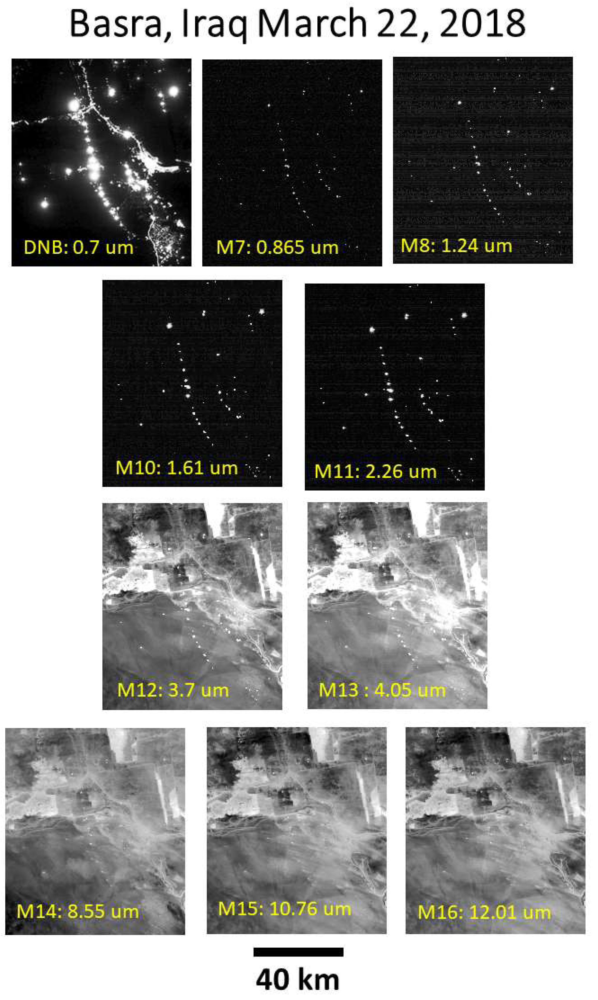
Figure 2.
Grayscale VNF 2012-2025 summary detections grid with the flare detection from the 2024 annual flare catalog of a large flare cluster with extensive glow in Venezuela. Locations of detected flares are marked with circles. Note the false flares identified in the glow.
Figure 2.
Grayscale VNF 2012-2025 summary detections grid with the flare detection from the 2024 annual flare catalog of a large flare cluster with extensive glow in Venezuela. Locations of detected flares are marked with circles. Note the false flares identified in the glow.
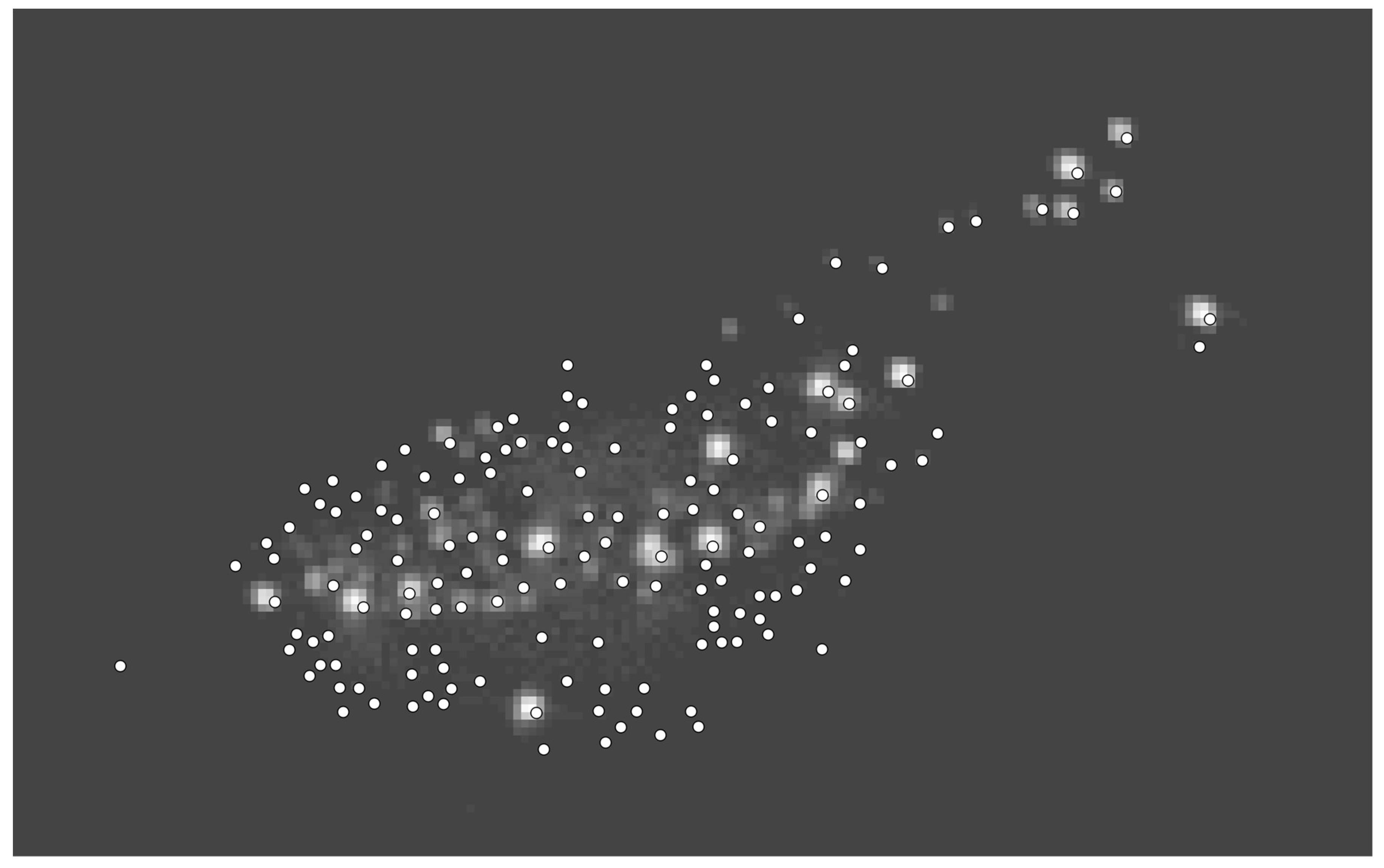
Figure 3.
Scattergram of grid cell average temperatures versus percent frequency of detection for the three noise floor sampling areas.
Figure 3.
Scattergram of grid cell average temperatures versus percent frequency of detection for the three noise floor sampling areas.
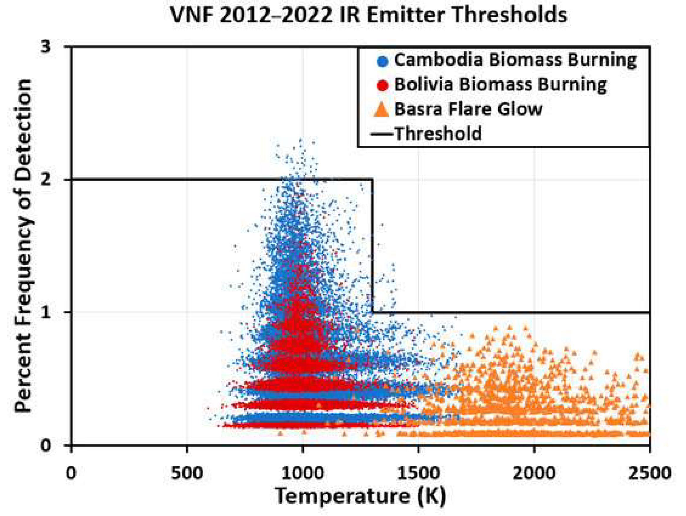
Figure 4.
Flowchart of the algorithm for building a high-resolution multiyear catalog of flares from VNF detections database.
Figure 4.
Flowchart of the algorithm for building a high-resolution multiyear catalog of flares from VNF detections database.
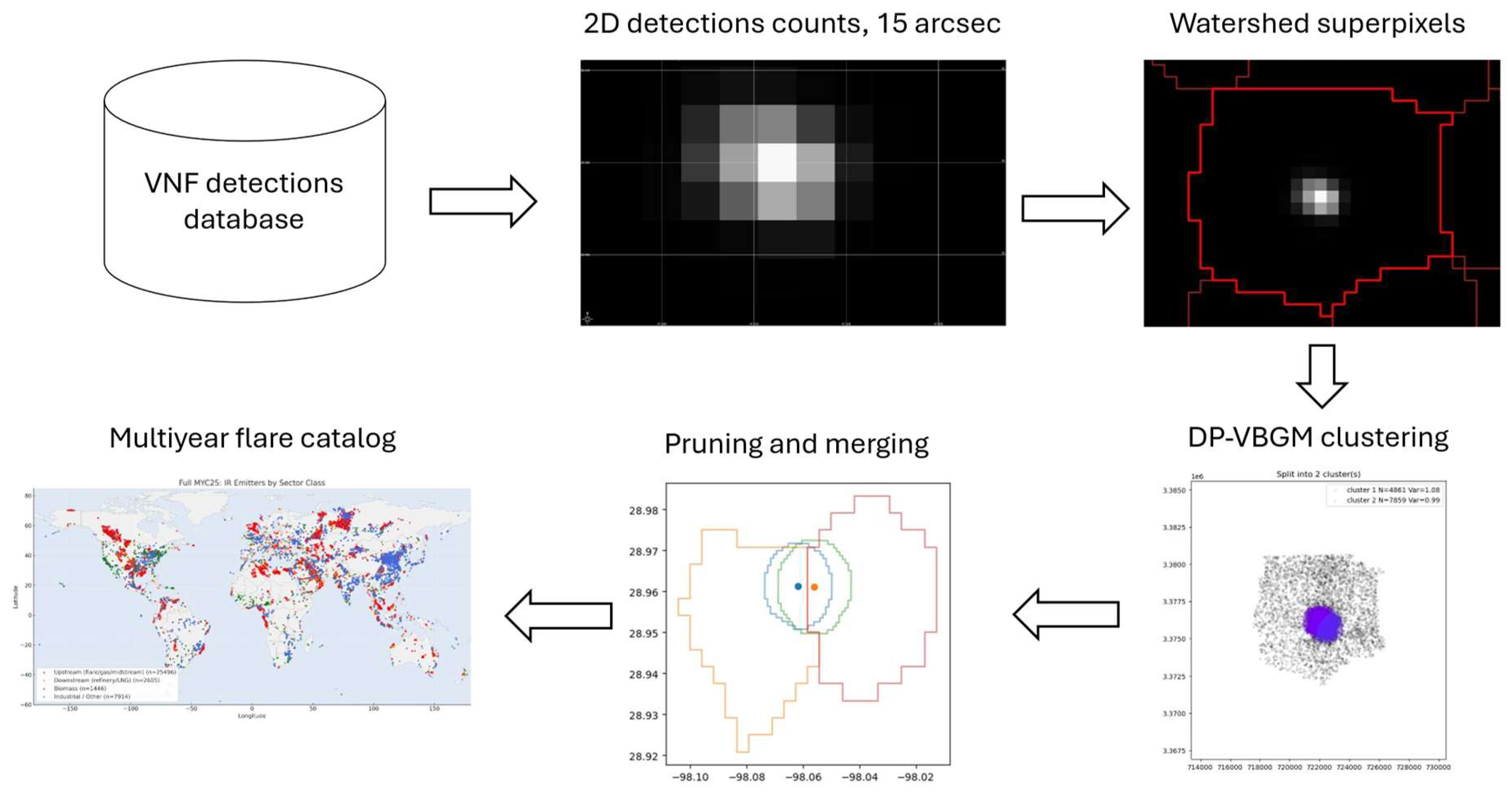
Figure 5.
High-resolution daytime satellite image (top) and the corresponding VNF-detections count grid (bottom) for a region with multiple flares in Basra, Iraq.
Figure 5.
High-resolution daytime satellite image (top) and the corresponding VNF-detections count grid (bottom) for a region with multiple flares in Basra, Iraq.
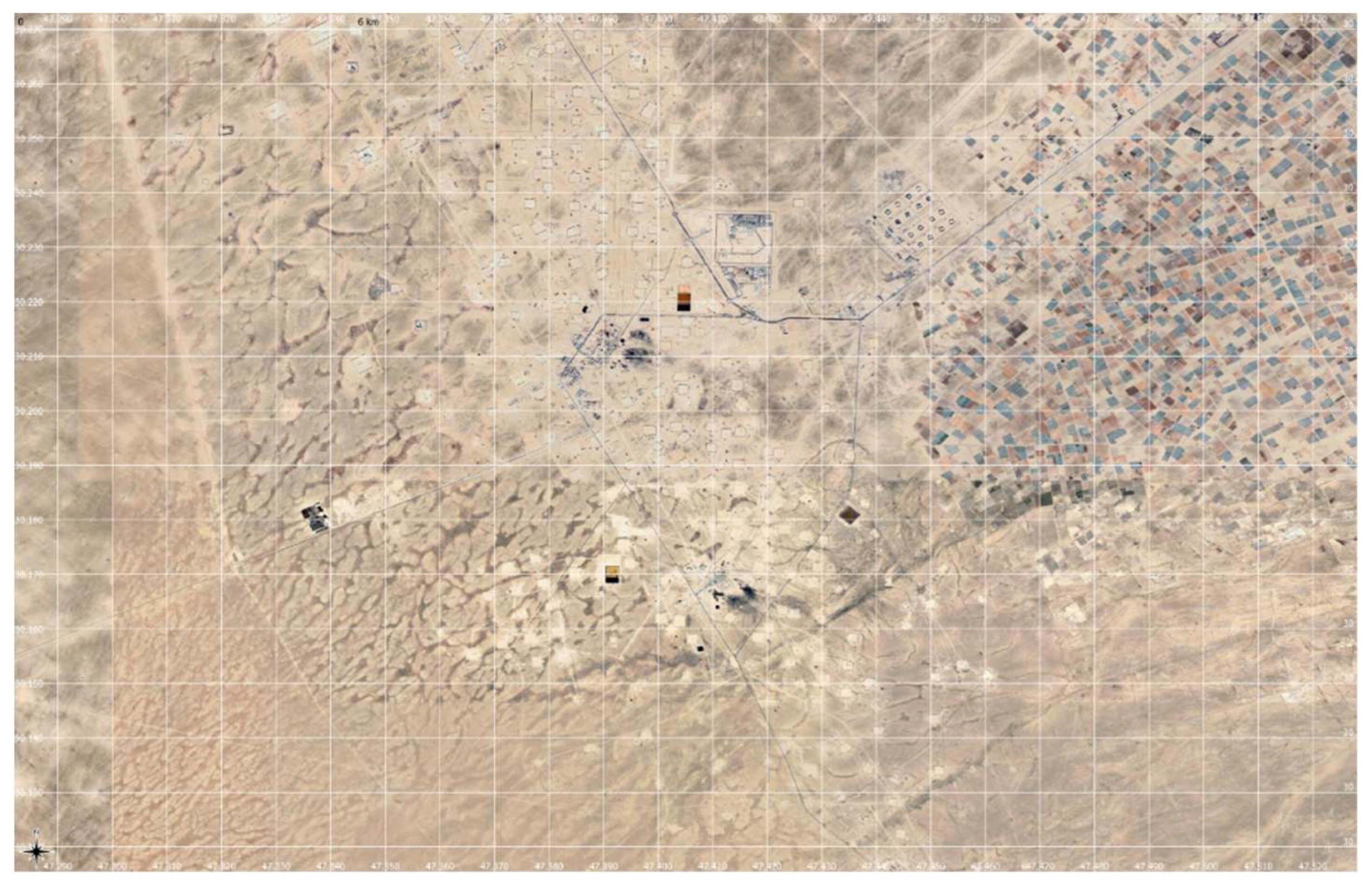
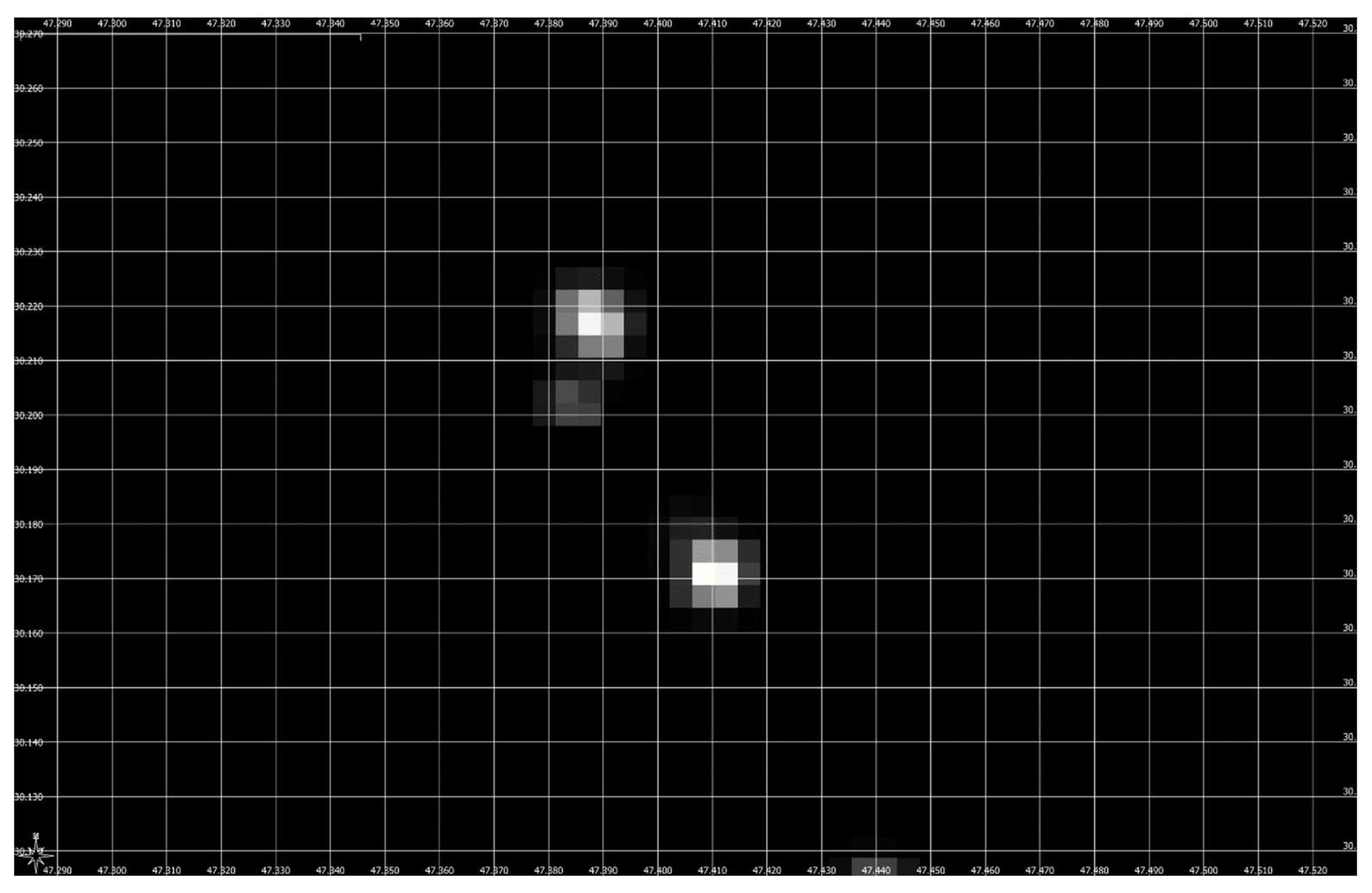
Figure 6.
Watershed segmentation result for the flaring region in Basra. Superpixel boundaries are shown in red. For comparison, flare boundaries from the annual 2024 catalog are shown in green.
Figure 6.
Watershed segmentation result for the flaring region in Basra. Superpixel boundaries are shown in red. For comparison, flare boundaries from the annual 2024 catalog are shown in green.
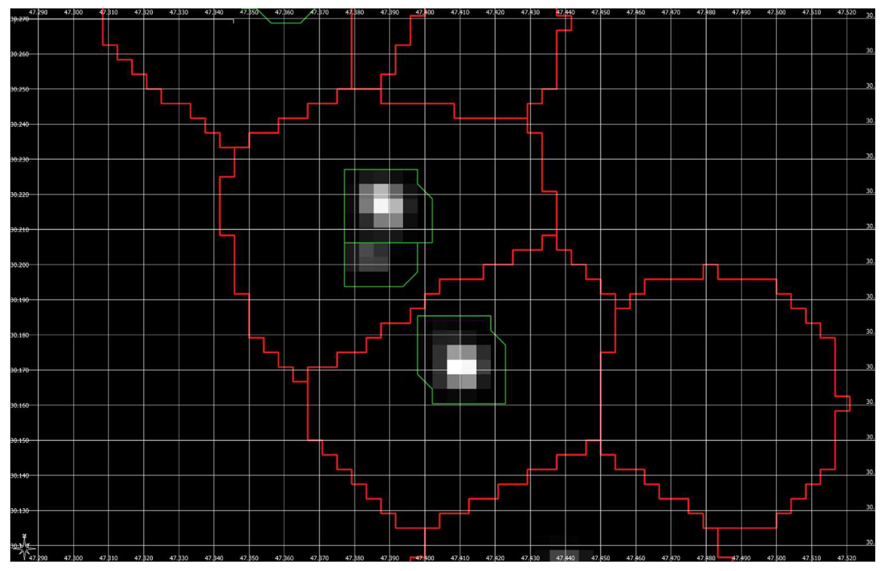
Figure 7.
Super-resolution clustering within a single waterpixel. Left: Detection probability density map built from a 2D histogram of VNF detections (100 m grid cells). Warmer colors mark higher densities, revealing a compact, rotated-square hotspot characteristic of point-source flares. Axes are local UTM easting/northing (m). Right: All VNF detection centers (gray points) within the waterpixel reprojected to the same UTM frame and partitioned by a DP-VBGM into four compact subclusters (colored fills).
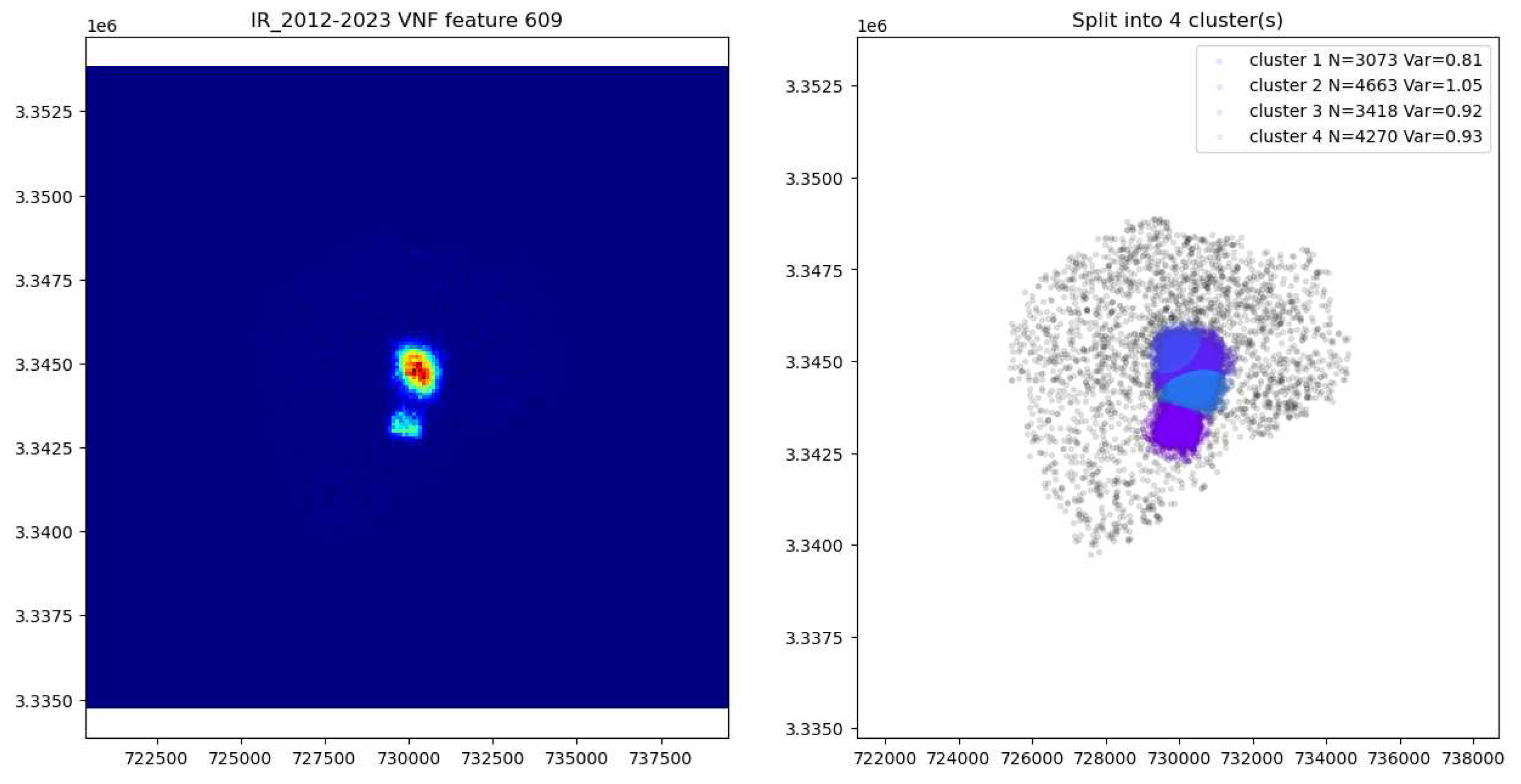
Figure 8.
The red polygons outline the “bubble vectors” of each flare stack after DP-VBGM unmixing. Partial overlaps indicate closely spaced emitters resolved within the waterpixel.
Figure 8.
The red polygons outline the “bubble vectors” of each flare stack after DP-VBGM unmixing. Partial overlaps indicate closely spaced emitters resolved within the waterpixel.
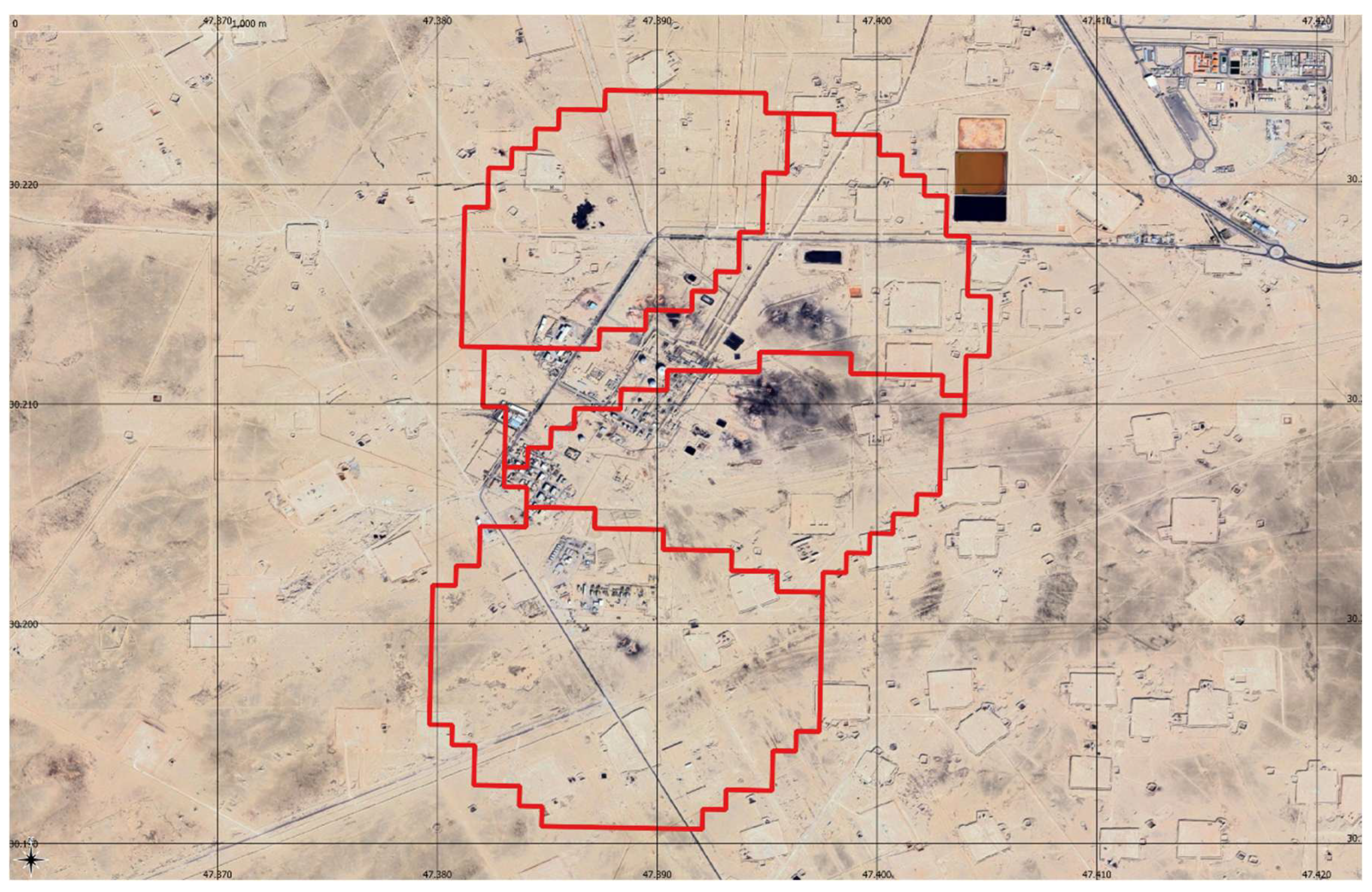
Figure 9.
Two types of super-resolution errors: colored outlines show “bubble vectors”; dots indicate centroids. Top: Clusters split at a superpixel boundary. Left: Pre-merge footprints from adjacent tiles. Right: Duplicate cluster boundaries on high-resolution daytime image. Bottom: Over-split flares found with DBSCAN. Left: Multiple polygons with centroids inside the merge radius 600 m. Right: Corresponding high-resolution image.
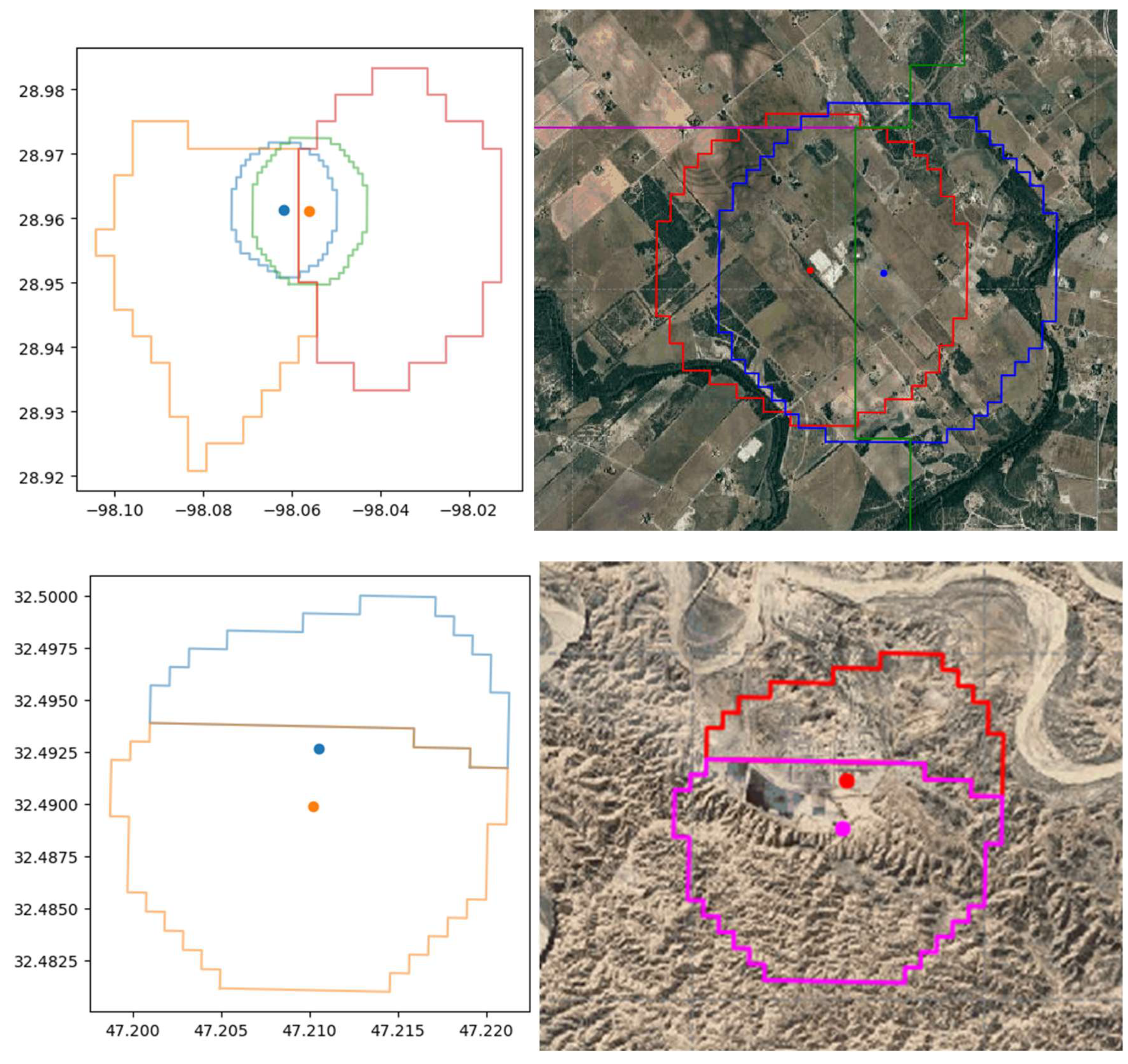
Figure 10.
Cleaned flare contours and centroids. Blue polygons show final footprints after duplicate merging and Voronoi re-contouring; red stars mark the centroids. One duplicate cluster was removed (compare with Figure 4), and the remaining flare-stack locations align with HRD ground truth within < 100 m (compare with 1,5 km VIIRS M-band pixel size).
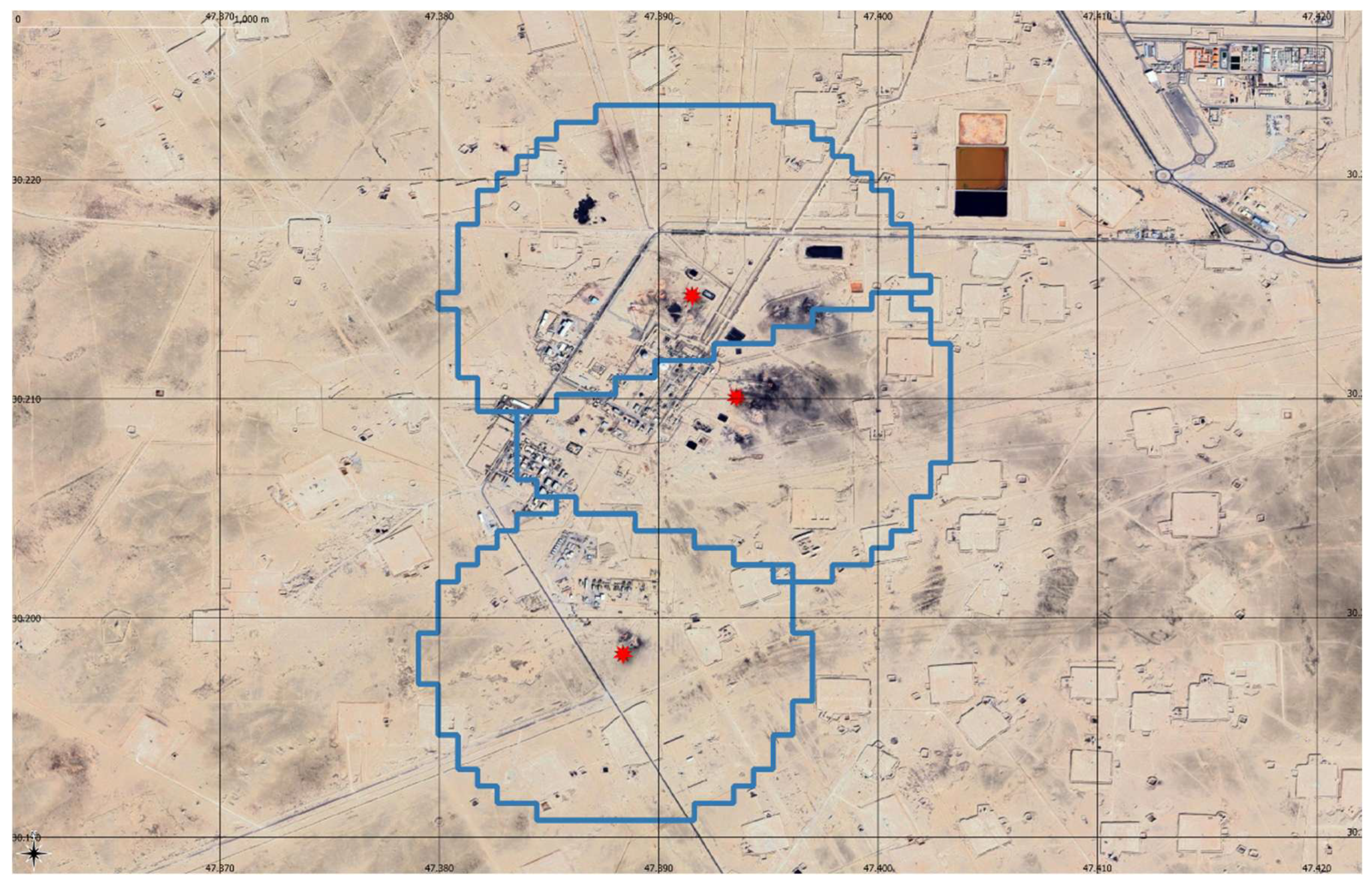
Figure 11.
Interactive map, where users can click on pushpins to view AI-suggested labels, provenance matches, and supporting evidence to classify the newly detected persistent heat sources in MYC25 and its updates.
Figure 11.
Interactive map, where users can click on pushpins to view AI-suggested labels, provenance matches, and supporting evidence to classify the newly detected persistent heat sources in MYC25 and its updates.
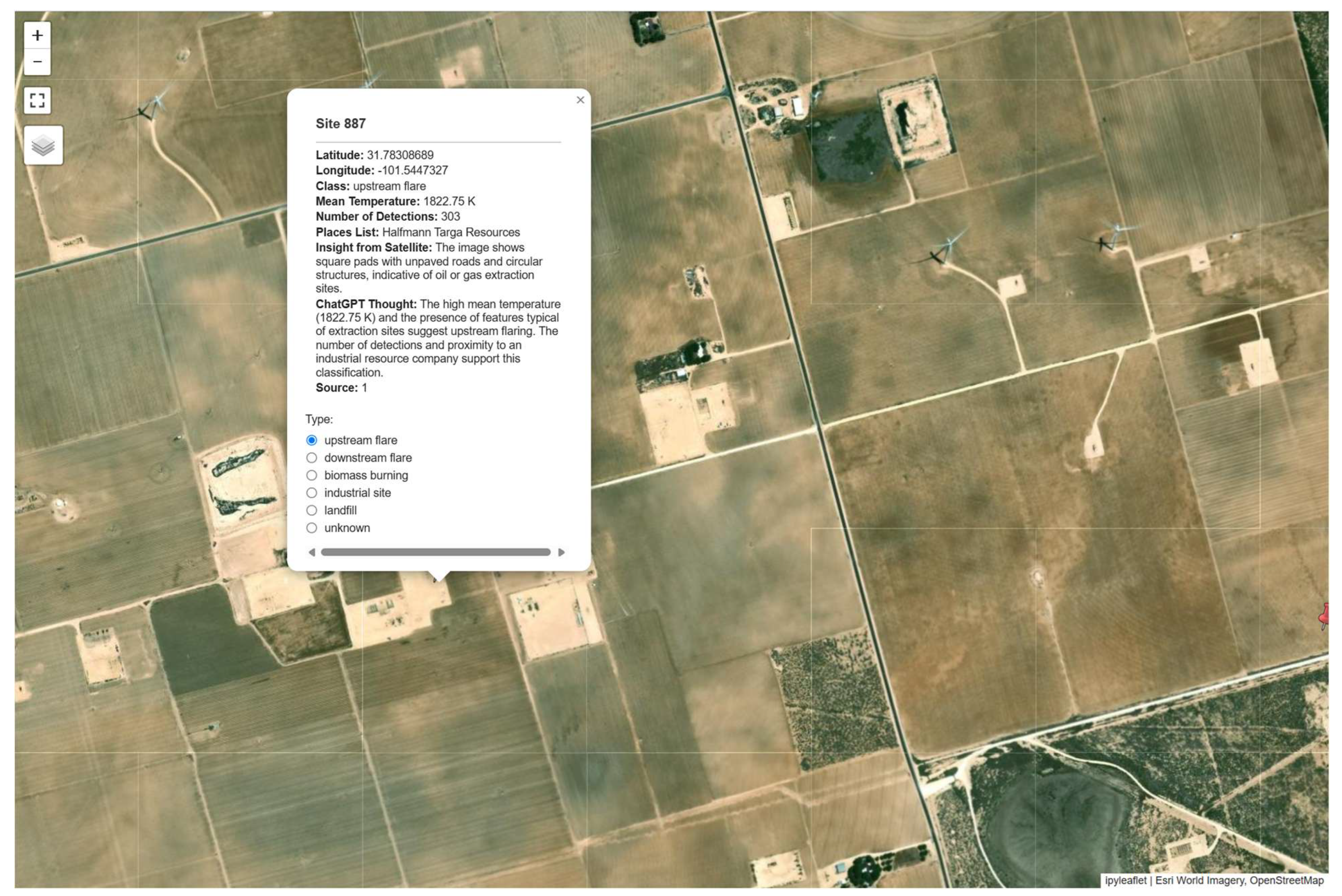
Figure 12.
Global inventory of MYC25 IR emitters shows characteristic regional patterns: upstream concentrations in major oil provinces, downstream clusters near refining and LNG hubs, and biomass burning in agricultural belts.
Figure 12.
Global inventory of MYC25 IR emitters shows characteristic regional patterns: upstream concentrations in major oil provinces, downstream clusters near refining and LNG hubs, and biomass burning in agricultural belts.
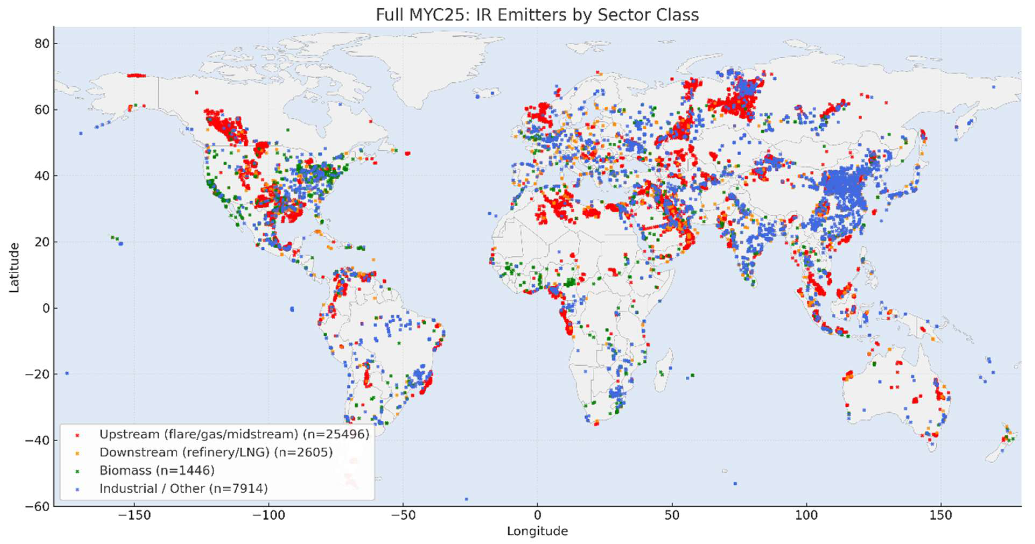
Figure 13.
Breakdown of the IR emitters in the multiyear catalog by type.
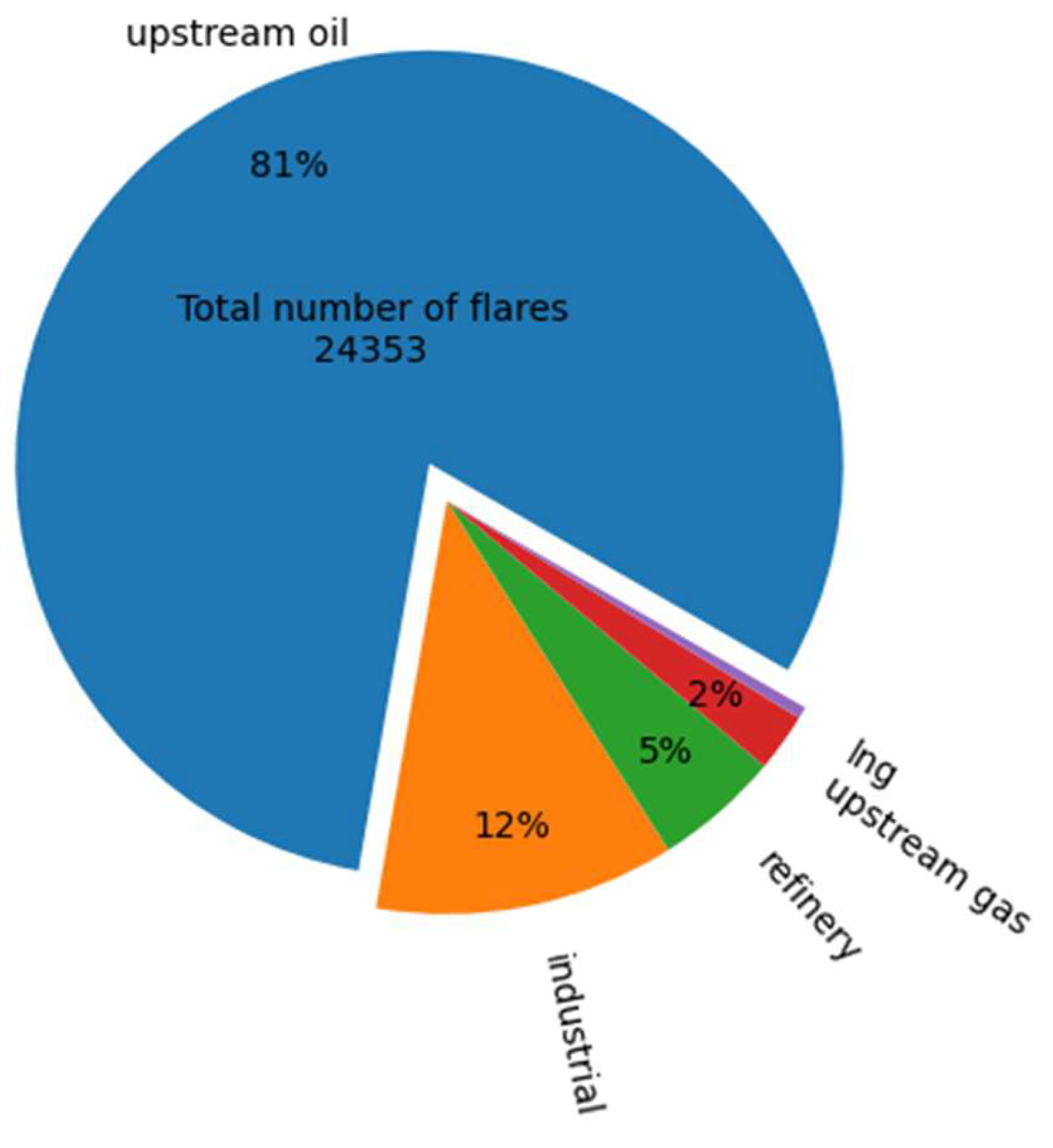
Figure 14.
Improved sensitivity for small flares in Colorado recovers numerous infrequent flares. Flares in the MYC25 are shown in green, flare contours (“bubble vectors”) for VNF detections are in blue, and flares from Annual 2024 catalog are shown in red.
Figure 14.
Improved sensitivity for small flares in Colorado recovers numerous infrequent flares. Flares in the MYC25 are shown in green, flare contours (“bubble vectors”) for VNF detections are in blue, and flares from Annual 2024 catalog are shown in red.
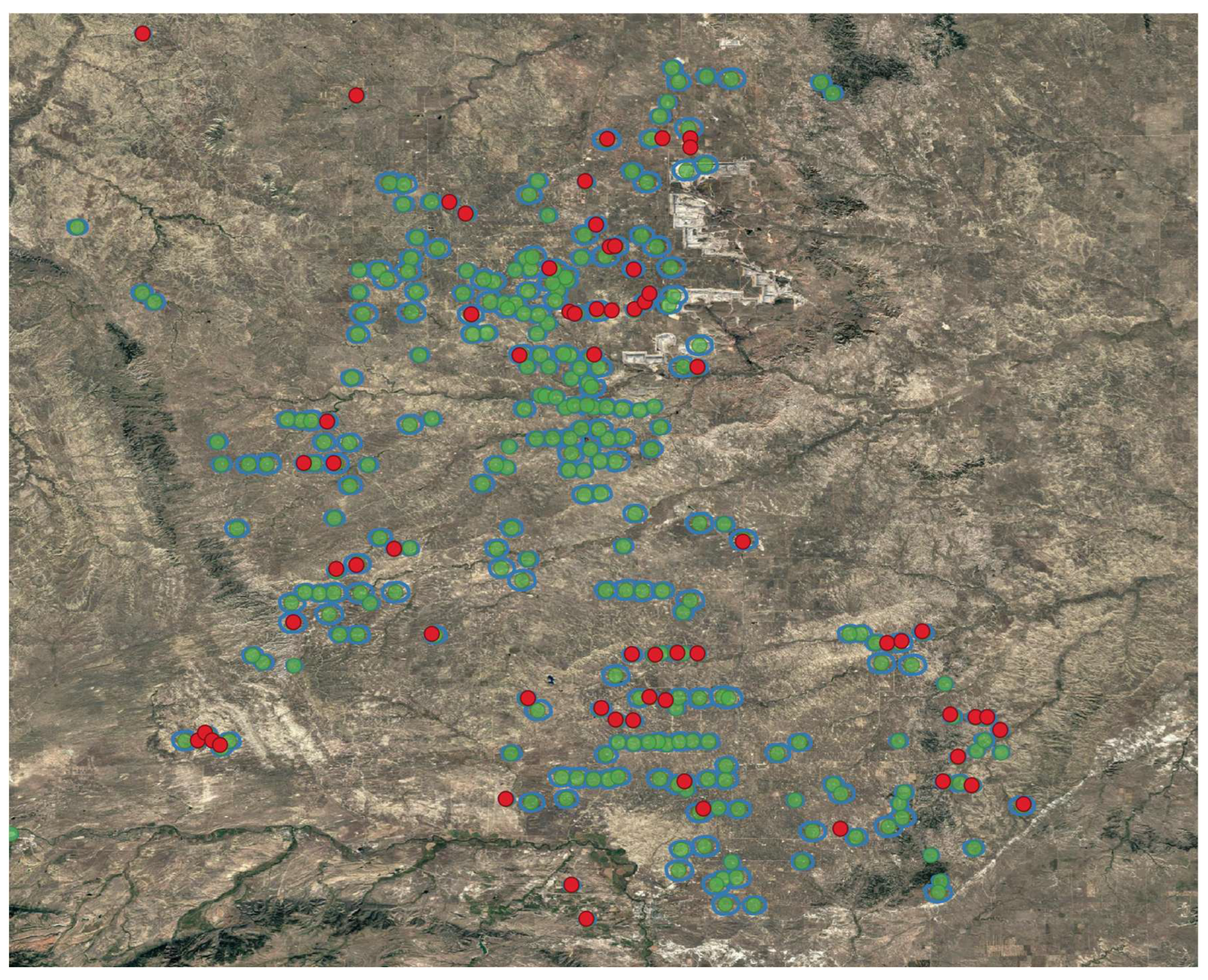
Figure 15.
Improved selectivity in region with very large flares in Venezuela removes false positives around large stacks. Flares in the new MYC25 are shown in green, flare contours (“bubble vectors”) for VNF detections are in blue, and flares from Annual 2024 catalog are shown in red. Many spurious VNF detections from atmospheric glow in the Annual 2024 catalog were identified as flares.
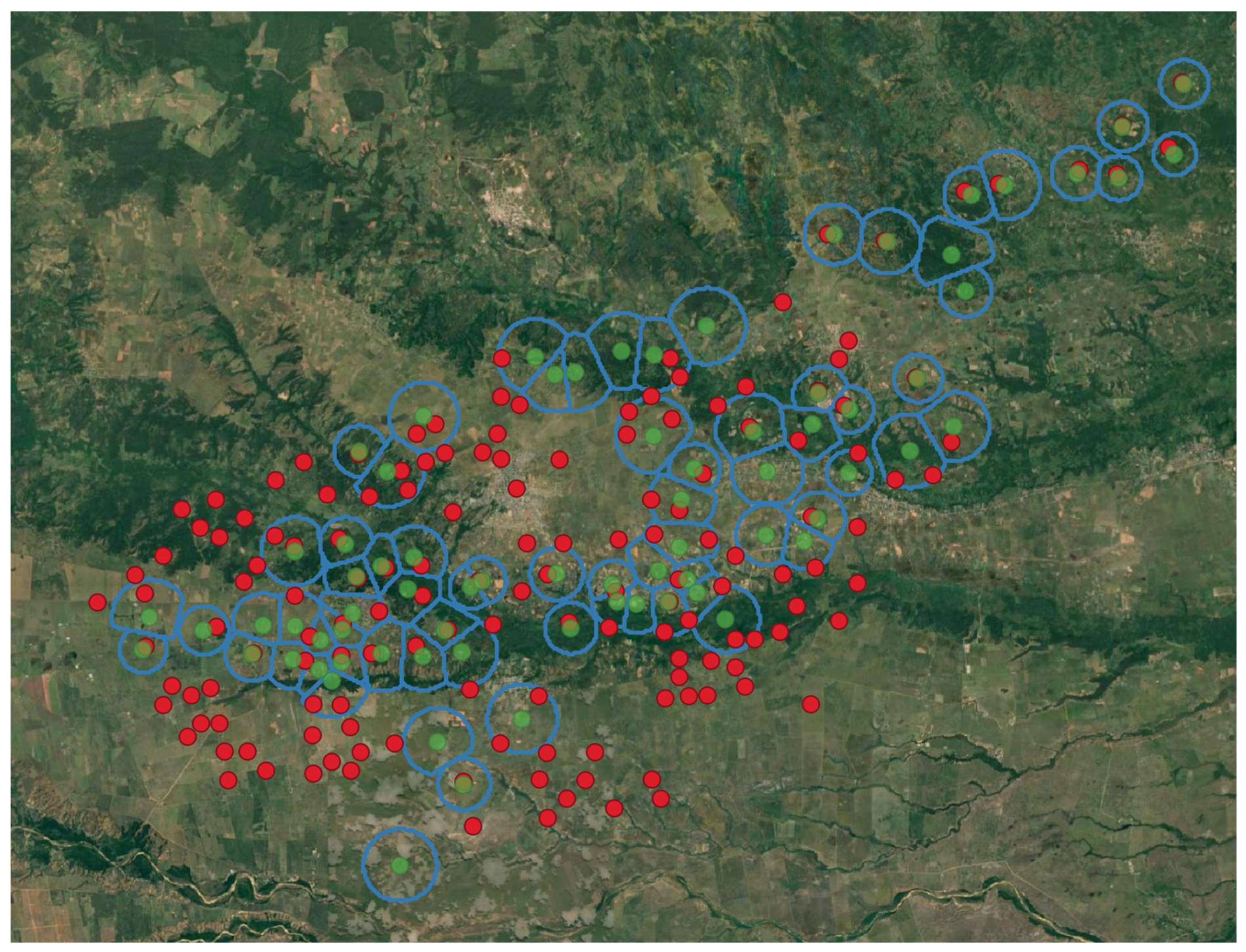
Figure 16.
Difference in number of upstream active (≥1 detection) flares in 2024 (single year) reported in MYC25 (blue bars) and Annual 2024 (orange bars).
Figure 16.
Difference in number of upstream active (≥1 detection) flares in 2024 (single year) reported in MYC25 (blue bars) and Annual 2024 (orange bars).
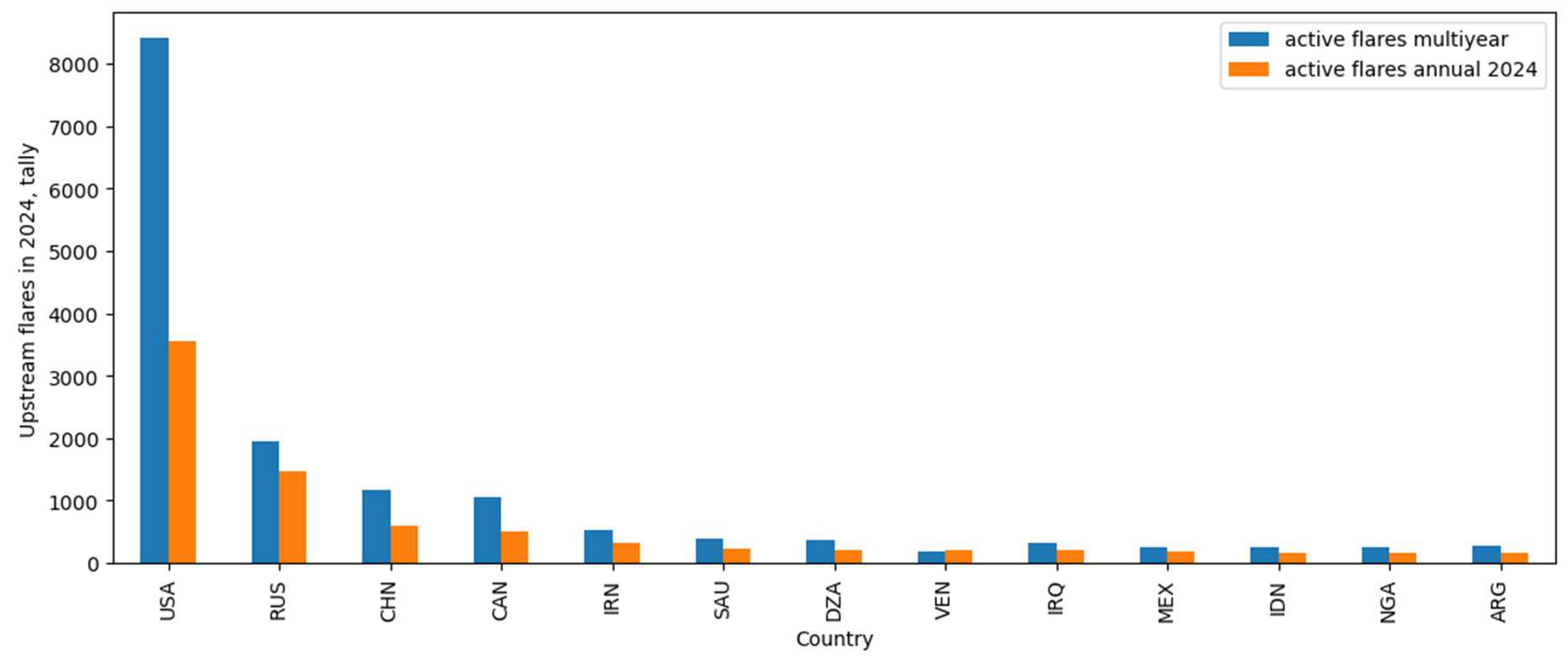
Figure 17.
Distribution of detection counts and duty cycle for upstream flares active in 2024 from the multiyear (MYC25; gold) and the Annual 2024 (blue) catalogs.
Figure 17.
Distribution of detection counts and duty cycle for upstream flares active in 2024 from the multiyear (MYC25; gold) and the Annual 2024 (blue) catalogs.
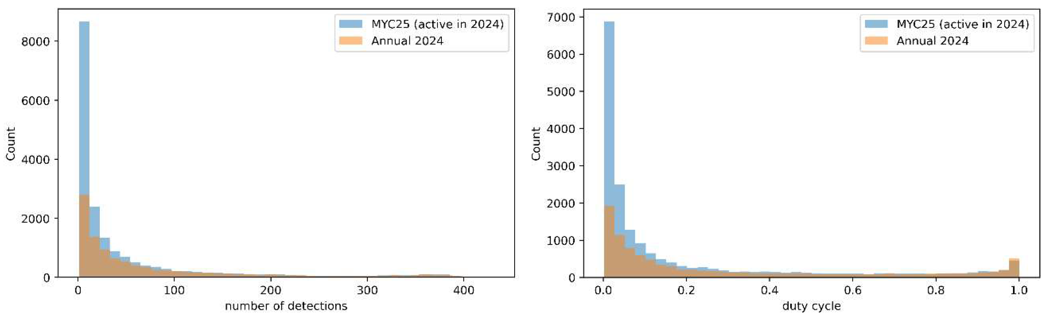
Figure 18.
Nearest neighbor association distance between the MYC25 and legacy MYC22, Annaul 2024 catalogs (distance threshold ≤300 m). The MYC25 to MYC22 curve is sharply concentrated at small offsets, indicating tight cross-catalog localization, whereas the broader MYC25 to Annual 2024 distribution reflects less precise watershed feature-based centroids in Annual 2024.
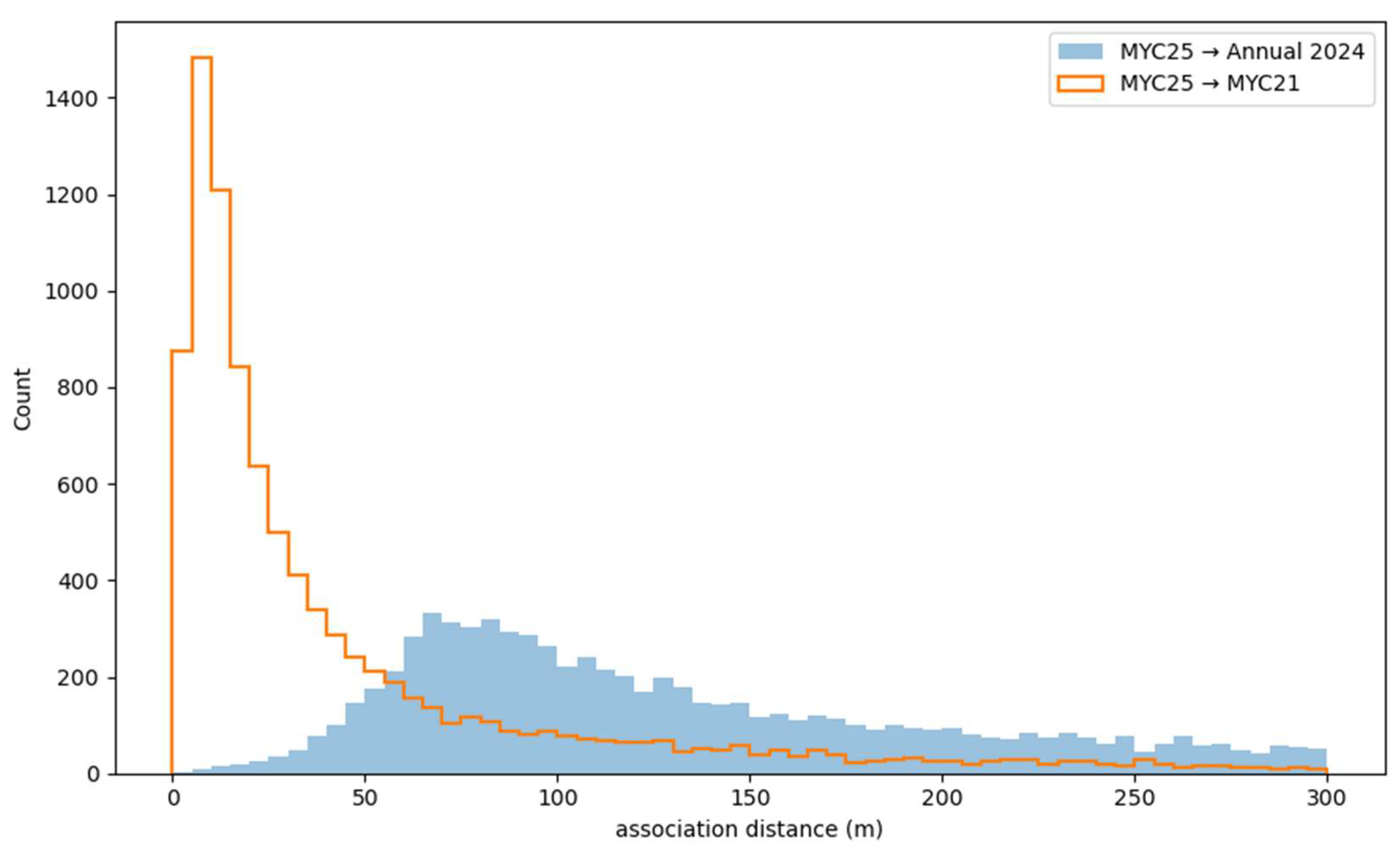
Figure 19.
Empirical spacing of stacks that MYC25 actually resolved inside sites that the Annual catalog considers as one feature.
Figure 19.
Empirical spacing of stacks that MYC25 actually resolved inside sites that the Annual catalog considers as one feature.
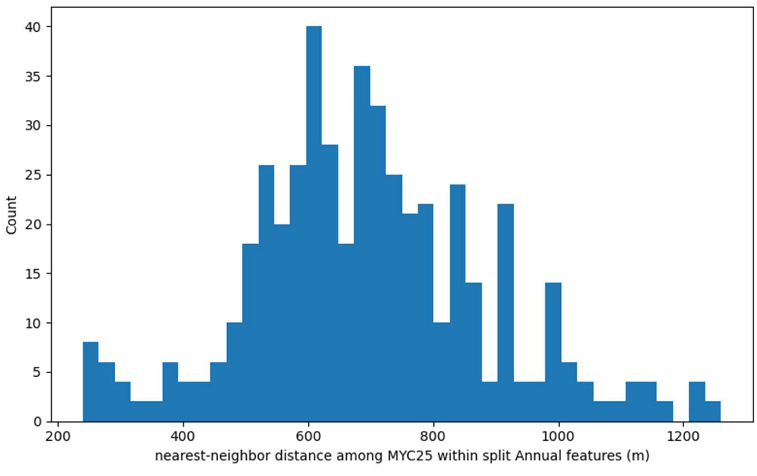
Figure 20.
Distribution of LNG liquefaction terminal to nearest MYC25 flare distance. Single outlier T0216 are excluded from the plot for clarity.
Figure 20.
Distribution of LNG liquefaction terminal to nearest MYC25 flare distance. Single outlier T0216 are excluded from the plot for clarity.
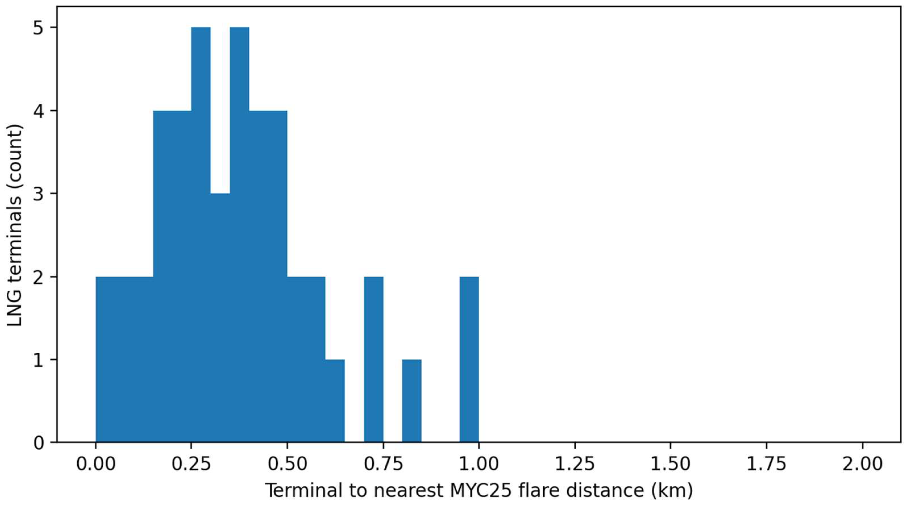
Figure 21.
Global distribution of IR emitters from the quarterly update, by mean temperature Tmean.
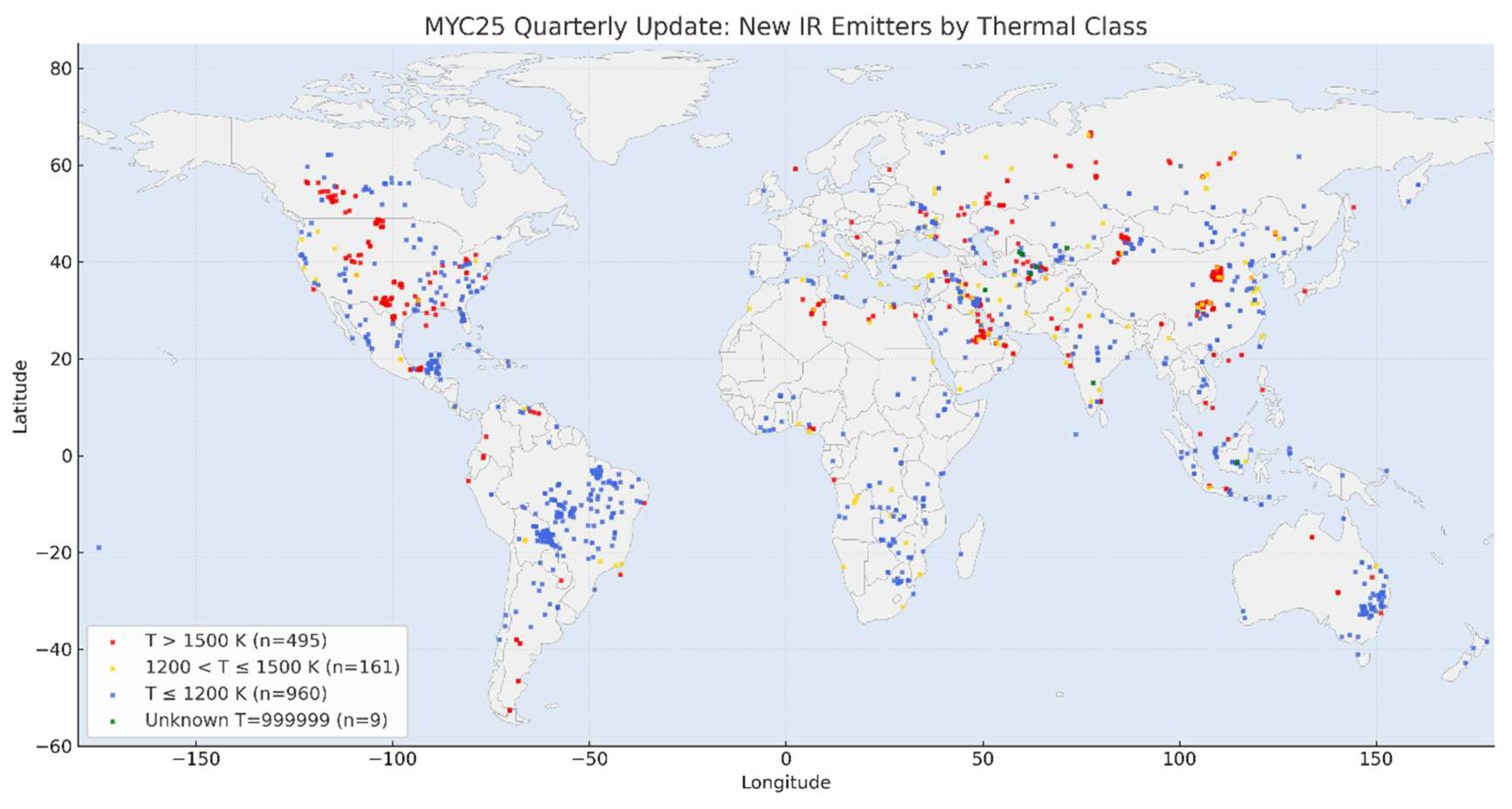
Figure 22.
Temperature distribution of newly detected IR emitters (April–July 2025).
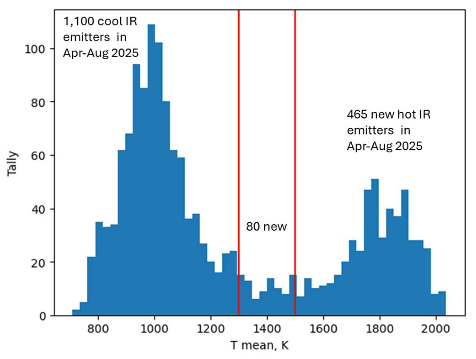
Figure 23.
Country-level impact of switching from Annual to MYC25 for BCM estimates in 2024. Six panels (2×3) show the combined change in flared gas (Δ BCM = MYC − Annual) and its decomposition for the largest-flaring countries in 2024 (ordered to Mexico, inclusive). Top-left: Combined absolute Δ; top-right: relative Δ (% of Annual). Bottom panels: component contributions—1:1, Split Δ (1:many plus folded merges/many-to-many), Missing Δ (Annual-only, typically glow/overspill removed by MYC), and New Δ (MYC-only detections). Positive bars indicate increases in MYC25; negative bars indicate reductions relative to Annual.
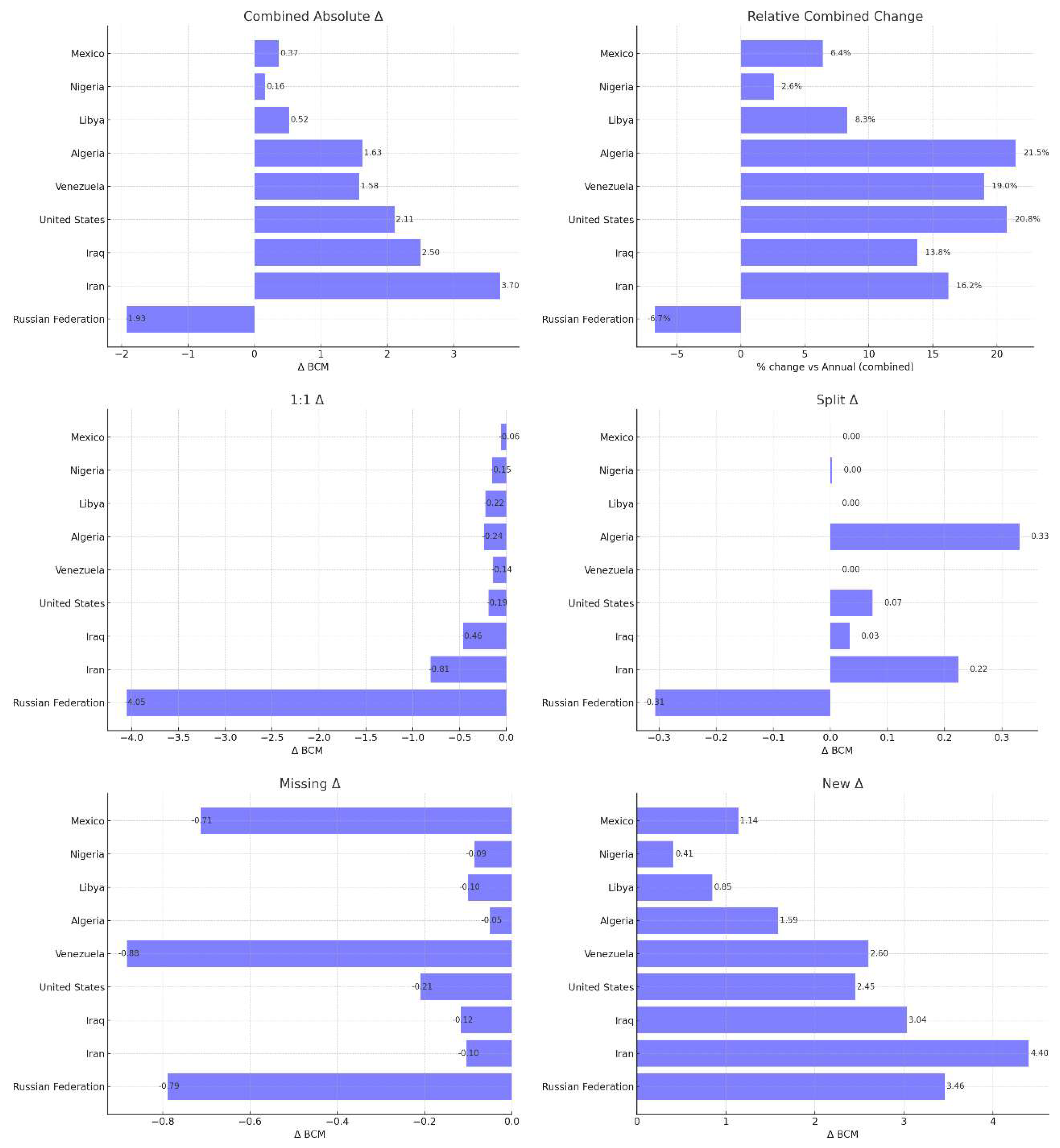
Figure 24.
Centroid association vs. boundary-aware matching for two adjacent flares (68.1707N, 55.3710E, northern Russia). High-resolution imagery with the Annual catalog’s watershed-style attraction contour (red) and the MYC25 catalog’s Gaussian “bubble” polygons (amber) overlaid. Same color stars mark Annual and MYC flare centroids.
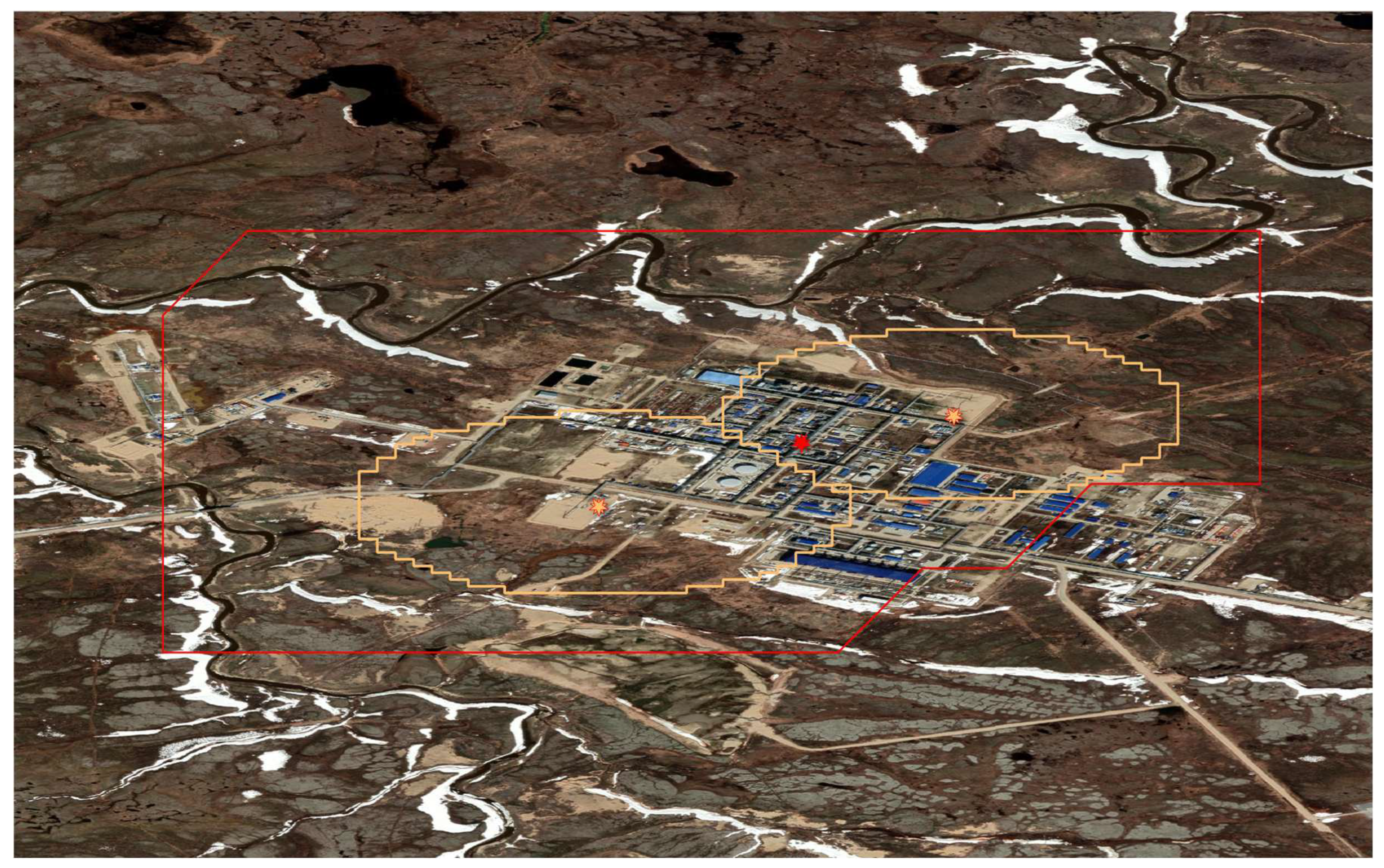

Table 1.
Known IR emitter tallies by type in MYC22.
| IR Emitter Type | Tally |
| Upstream gas flares | 13,449 |
| Downstream gas flares | 1535 |
| Metallurgy | 1732 |
| Industrial TBD | 1344 |
| Coal mines and power plants | 558 |
| Unknown | 528 |
| Wood processing | 297 |
| Landfills | 279 |
| Volcanoes | 92 |
| Cement factories | 83 |
| Unique | 4 |
| Greenhouses | 4 |
| TOTAL | 19,905 |
Table 2.
Detection and duty cycle metrics compared for MYC25 and Annual 2024 catalog.
| Metric | MYC25 (active in 2024) | Annual 2024 |
| N (active in 2024) | 18225 | 9881 |
| N detected median | 13 | 31 |
| N detected P25 | 4 | 10 |
| N detected P75 | 49 | 93 |
| N detected < 10 (%) | 45.61 | 26.22 |
| N detected > 50 (%) | 24.94 | 38.88 |
| Duty cycle median | 0.05 | 0.13 |
| Duty cycle P25 | 0.01 | 0.04 |
| Duty cycle P75 | 0.23 | 0.50 |
| Duty cycle < 0.2 (%) | 73.53 | 58.42 |
| Duty cycle < 0.5 (%) | 85.17 | 75.00 |
| Duty cycle > 0.8 (%) | 7.97 | 14.53 |
Disclaimer/Publisher’s Note: The statements, opinions and data contained in all publications are solely those of the individual author(s) and contributor(s) and not of MDPI and/or the editor(s). MDPI and/or the editor(s) disclaim responsibility for any injury to people or property resulting from any ideas, methods, instructions or products referred to in the content. |
© 2025 by the authors. Licensee MDPI, Basel, Switzerland. This article is an open access article distributed under the terms and conditions of the Creative Commons Attribution (CC BY) license (http://creativecommons.org/licenses/by/4.0/).
Copyright: This open access article is published under a Creative Commons CC BY 4.0 license, which permit the free download, distribution, and reuse, provided that the author and preprint are cited in any reuse.


