Submitted:
30 October 2025
Posted:
03 November 2025
You are already at the latest version
Abstract
This paper explores the application of mobile sensor networks in cow herds, focusing on the challenge of achieving local communication under minimal computational constraints such as restricted locality, limited memory, and implicit coordination. To address this, we propose a high connectivity based sensor network scheme that enables individual sensors to self-organize and dynamically adapt to topological variations caused by cow movements. In this scheme, each sensor acquires local distribution data from neighboring sensors, identifies those with high connectivity, and forms a local sub-network with a star topology. The overlap of these local sub-networks results in a globally interconnected mesh topology. Furthermore, information exchanged through broadcasting and overhearing allows each sensor to incrementally update and adapt to dynamic changes in its local network. To validate the proposed scheme, a custom wireless sensor tag was developed and mounted on the necks of individual cows for experimental testing. Furthermore, large-scale simulations were performed to evaluate performance in herd environments. Both experimental and simulation results confirmed that the scheme effectively maintains network coverage and connectivity under dynamic herd conditions.
Keywords:
mobile sensor network
; local communication
; high-degree connectivity
; custom wireless sensor tag device
; monitoring application
; herd of pastured cows
1. Introduction
Recently, the adoption of ICT and IoT technologies [1,2,3] in the livestock industry has been promoted to improve operational efficiency and reduce labor demands. Commercial devices, including estrus detectors [4,5], birth monitors [6], and feeding robots [7,8], are increasingly employed in beef cattle production, replacing traditional manual tasks. Early detection of illness or stress in cattle is considered feasible through behavioral analysis aimed at identifying abnormal patterns.
Various approaches have been explored to monitor and identify abnormal behaviors in cows [9,10]. Behavior analysis using a single sensor has been explored through several approaches such as attaching triaxial accelerometers and magnetometers to cows to monitor movements [11,12,13] or installing communication sensors in cowsheds to infer behavior from radio signal strength [14,15,16]. Other approaches include using depth cameras to monitor calving [17,18] and microcontrollers to track heart rate and body temperature [19,20]. Additionally, management systems have been proposed for large-scale environments, such as pastures, by implementing dedicated communication infrastructures. Examples include systems that detect estrus cycles using communication sensors to form behavior-monitoring networks [21,22], as well as methods for managing pasture areas by analyzing the movement patterns of GPS-equipped grazing cows [23,24]. Based on these studies, communication-enabled sensors can be deployed to implement management systems in large-scale environments such as pastures. Despite their innovative contributions, most existing monitoring approaches have primarily focused on individual cow behavior, with limited exploration of interactions and social relationships within the herd. Furthermore, the specific types of information necessary for mechanistic visualization of interactions among the cows remain poorly defined. Unfortunately, few studies have investigated stress assessment based on social interactions, such as mutual licking, or examined behavior at the group level.
To address these limitations, this study proposes a communicative interaction scheme for visualizing interactions among cows in a freely grazing herd as illustrated in Figure 1. Specifically, we devise a network using communication sensors mounted on cows, utilizing radio signal strength to facilitate both individual identification and group behavior analysis in a grazing environment. In this paper, we aim to visualize interactions among cows by constructing a network based on mutual communication between sensor devices attached to them. To achieve this, we address two main challenges: an engineering challenge, involving the configuration of a sensor-based communication network, and an agricultural challenge, involving the analysis of social relationships among cows. To tackle the engineering challenge, sensors are attached to each cow, and they are identified based on communication reliability with nearby cows, enabling the generation of local networks. To cope with the agricultural challenge, a friend network is established by limiting the communication range to emphasize relationships between cows that interact more frequently. The overall network is subsequently formed by overlaying the local and friend networks. To implement this concept in cows, we developed a neck-belt sensor tag and conducted evaluation experiments. Additionally, to assess the effectiveness of the proposed method in large-herd scenarios, we developed an in-house simulator and performed corresponding simulations.
This paper is structured as follows. Section 2 outlines our research problem and its definitions. Section 3 provides an explanation of the proposed solution. Section 4 details a custom neck-belt sensor tag. Section 5 shows the results from extensive experiments performed to evaluate the effectiveness and the performance of the proposed approach. Finally, Section 6 presents our conclusions.
2. Problem Statement
This paper considers a herd of n cows equipped with a wireless sensor-tag device as shown in Figure 2-(a). First, the communication range of each cow is defined as , and it is assumed that the range of is constant for . Moreover, the inter-communications within are used to exchange information and to obtain the radio wave strength between the sensor-tag devices. Specifically, sends a message to a neighboring cow in , and receives information including the radio wave strength (Figure 2-(b)). A specific range acquired is defined as . The range of is assumed to be constant for as in , namely is contained within . Although has its own initially, no specific roles such as leader, source, sink, and gateway are assigned. executes the same algorithm asynchronously but has no long-term state information.
We define as the state where can directly communicate with within . The set of cows within of is expressed as . refers to communication with cows outside via an intermediate cows. For example, in Figure 2-(a), if lies outside but is within of , then is a ’s cow of . The set of such cows is symbolized by . From , selects neighbors , forming the neighbor set (Figure 2-(c)). Furthermore, selects friends from based on , with the set defined as . The computation procedures for selecting and are described in the following section.
As shown in Figure 3, three message types are defined. (1) existence message , periodically broadcast by within and acknowledged by , (2) output message , sent to and acknowledged by , and (3) request message , sent to , which responds with . For simplicity, any message from is represented by . Next, a wait time is defined to evaluate connectivity. When broadcasts to , it measures the response interval . If receives a reply within , is considered within , forming part of . If no reply is received within , the connection is deemed broken, indicating that has moved outside .
The local network associated with is defined through its connections to . This yields a local graph , where is the set of vertices and is the set of undirected edges, excluding self-loops. The global herd network is then defined as . Next, based on , as illustrated in Figure 4, herd behavior is classified into four states: (mutual friends within ), (split into multiple local networks), (unified single network), and (isolated cow disconnected from the herd).
Based on the definitions and assumptions above, this paper addresses the monitoring of herd behavior through local communication interactions in a cow herd. To solve this problem, we propose a monitoring algorithm that visualizes herd behavior and inter-cow relationships using local network configurations and virtual distances. Specifically, selects and while forming through intercommunication within and . Herd behaviors and relationships are then inferred from , and by combining all , G is self-organized. Since G changes dynamically with herd movement, it requires partial modification, updating, and repair in response to behavioral changes. Details on the monitoring scheme are provided in the next section.
3. Monitoring Algorithm Based on Configuration
This section describes the monitoring algorithm for generating and maintaining based on herd behaviors. As shown in Figure 5, the algorithm consists of four functions: selection, selection, generation, and maintenance. Four of these functions are explained in this section. Based on this algorithm, the identification of herd behaviors is described in Section 4.2.
The algorithm takes , , and as inputs, and outputs , , , and . First, it checks whether is empty. If this is satisfied, and are selected, and is generated. If is not empty, the network maintenance is performed to accommodate changes in due to cow movements. After is generated or updated, a herd behavior is determined from its connection state. Finally, the outputs are broadcast to , and this process is repeated continuously.
Next, we define the terms used in the algorithm. The union of all transmitted by is . The correspondence between and via intercommunication is . denotes a candidate friend in computed from . Information from to through is expressed as , and represents the minimum received signal strength. Information held by at time t is , with the previous time step defined as ; for simplicity, the time indices are omitted in subsequent explanations.
3.1. Selection
The first computation function selects and consists of two steps: information gathering from and neighbor searching.
3.1.1. Acquisition of Information
In the first step, receives from . It first checks whether is sent by and whether the response from occurs within . If both conditions are satisfied, is retained in and sends an updated . Using and within , calculates the state of beyond . For example, in Figure 6, , , and are within , and , , and are beyond . When connects to , , and , and obtains , a correspondence table is organized as mapping elements of (right side of Figure 6). From and , is calculated:
By calculating , estimates information about cows beyond its . The intercommunication correspondence between and is defined as and , respectively. Here represents connections from elements of to elements of as shown on the left in Figure 7-(a).
, also represented by like , is shown on the right in Figure 7-(a). Conversely, represents connections from elements of to elements of as shown on the left in Figure 7-(b).
Similarly, is represented as as shown on the right in Figure 7-(b). The combination of and defines the connections from to via and is expressed:
By using the composition of and , can estimate the connection state of .
3.1.2. Calculation
The second step selects using and obtained from . First, identifies the element of with the highest number of to cows in , defined as , and selects it as the first neighbor . The corresponding elements in and are then removed. This process is repeated to select the second neighbor and subsequent neighbors, each time removing the corresponding elements, until is empty (the right side in Figure 8).
3.2. Selection
The second computation function, called friend sorting, selects and determines .
3.2.1. Calculation
The first step is to obtain from the information on as mentioned in Section 3.1.1. If both and are within the range (Section 2), the corresponding element of is selected as ; otherwise, is set to empty. Here, denotes of elements in . For example, if and are in ’s (see the left side of Figure 9), the step checks whether from to , and from both and to are mutually within . Elements satisfying this criterion (, ) are selected as (see the right of Figure 9).
3.2.2. Calculation
The second step is to extract from obtained in the previous step. To begin, the procedure checks whether is non-empty. If it is satisfied, is calculated under the condition .
Next, if the calculated is the minimum value, it is assigned to , and is computed accordingly.
Finally, the computed as shown in Figure 10, is designated as the primary member of .
If , it assigns the minimum to , and computes as the primary element of .
If multiple values are equal, the corresponding are all designated as main members of .
3.3. Generation
The third computation function generates . The input of is , and the output is . Vertices consist of and its selected , expressed as , forming the set . Each edge between and is defined as , and denotes the connection of . As shown in Figure 11, when is selected as , the corresponding local network of is generated. After constructing , broadcasts and and exchanges this information with .
3.4. Maintenance
The fourth computation function, network maintenance, addresses changes caused by cow movement. These changes occur in three states: (1) only changes (Figure 12-(a)), (2) only changes (Figure 12-(b)), or (3) only changes (Figure 12-(c)). This function consists of five steps: information acquisition, candidate calculation, calculation, calculation, and reconfiguration.
3.4.1. Information Acquisition
3.4.2. Calculation
In the second step, is obtained in Section 3.2.1. If both and the elements are within , the updated is selected as ; otherwise, remains unchanged.
3.4.3. Calculation
In the third step, using calculated in Section 3.2.2, if for the newly computed is non-empty, the elements of and are compared. Next, is calculated using Eq. (5) when . If the resulting is minimal, it is assigned to . The new is then compared with the previous value; if it remains minimal, a new is computed using Eq. (6) and becomes the member of . If is empty, the minimal is assigned to after compared with the previous value, and a new is used to update via Eq. (7).
3.4.4. Calculation
The fourth step investigates neighbors described in Section 3.1.2, using and computed from the first step. first selects the element of with the highest number of edges to cows in (Eq. (3)) as the first neighbor. The corresponding elements in and are then removed. This process is repeated to select subsequent neighbors until is empty.
3.4.5. Reconfiguration
In the fifth step, is partially reconstructed using updated information, following the same procedure as the generation function. First, the cow’s state is determined based on its movement. If changes, the vertices of and newly selected are updated in . If changes, the connections between the new and members are recalculated using Eq. (4). Similarly, variations in immediately trigger reconfiguration of its connections with . This partial reconfiguration maintains without requiring a full rebuild.
4. Development and Operational Experiments of Wireless Sensor Tag Device
This section describes a wireless sensor tag device (hereafter referred to as the “sensor tag”) that implements the above algorithm for identifying herd patterns in cows.
4.1. Design Concept of Wireless Sensor Tag Device
The development process of the tag is divided into three parts: the components, the frame of attaching the tag to each cow, and the monitoring system through a server receiver. These elements are required for the execution of the algorithm explained in Section 3. First, the tag should support mutual communication with acquisition. Second, the tag should execute computations using the algorithm. Third, the tag should temporally store data received from other tags.
Next, from an installation standpoint, two key requirements should be met: battery-powered operation and protective housing. Battery operation is essential since external power cannot be used when the tag is attached to cows. The tag-housing frame protects the tag, and allows for attachment to a wearable neck belt. In addition, monitoring requires a server connection to confirm tag status and collect data.
4.2. Development of Wireless Sensor Tag Device
To validate the algorithm, as illustrated in Figure 13, we developed a server tag and a sensor tag consisting of two parts: an electronic module and a frame. Details are presented in the following subsections.
4.2.1. Electronic Modules
The electronic module comprises a communication unit and an arithmetic unit. First, for the communication unit, we use the ESP32-WROOM-32 microcontrollers (Espressif Systems, China). This module combines Wi-Fi and Bluetooth in a single unit and is suitable for wireless communication. Furthermore, the module contains a 32 oscillator and a 2.4 band antenna. The wireless standard used is Wi-Fi: 802.11 b/g/n. Figure 14 shows the structure of the packets used for communication. As shown in Figure 3, for communication, two packet types are established: fixed-length and varying-length, depending on the type of messages. The packet format shown in Figure 14-(a) is used for , , and . On the other hand, Figure 14-(b) illustrates the packet format used for broadcasting . Specifically, in the packet, data length refers to the length of the data, the command defines the action for each message, source is the sender’s , target is the recipient, and data carries the information for the command.
Second, the arithmetic unit uses an ESP32 microcontroller, a low-cost, low-power SoC with an Xtensa dual-core 32-bit LX6 processor (240 MHz, <600 DMIPS) and 520 KB SRAM. A micro SD card slot and a Real-Time Clock (RTC) module (SparkFun Electronics, Colorado, USA) store the algorithm’s data along with transmission and reception timestamps.
Finally, is obtained via the tag’s Wi-Fi module. The module first scans the network to identify the number of tags within , after which an is assigned to each detected tag. The scanned values, including , are then logged to the micro-SD card.
4.2.2. Frame Unit
The frame unit, powered by three AA batteries (4.5 V), houses the electronic module in a PLA resin case with a waterproof lid and neck-belt buckle. The module and batteries are arranged in a two-layer structure (Figure 15). Module size: 55×45×20; frame size: 75×100×55 (including buckle). Figure 16 shows the assembled tag.
4.2.3. Monitoring Unit: Sever System
As shown on the left-hand side of Figure 13, the monitoring device consists of a computer and an electronic module. The LG gram computer is an Intel(R) Core Ultra 7 155H CPU with Microsoft Windows 11 Home. The Microsoft Visual Studio C++ 2022 environment of Visual Studio Code was used for the algorithm. A module is attached to the computer to receive the tag information.
4.2.4. Determination of Herd Behavior Pattern
For the monitoring of herd behaviors as explained in Section 2 (Figure 4), the determination function for five types of group patterns is described. We first check whether is an empty set. If , the cow is classified as , indicating it is isolated from the herd. If , the herd is evaluated as a single herd. If all cows belong to a single network, the herd is classified as . If the network is disconnected, with multiple sub-networks, the herd is classified as . Finally, if cows within the herd are mutually within each other’s and maintain a state of mutual friendship, the herd is classified as .
4.3. Preliminary Experiments of RSSI and Network Generation
The signal strength of the developed tag decreases with distance. To examine this attenuation, preliminary experiments were conducted using ten sensor tags and one server tag. The server tag was fixed in position, while the sensor tags were placed at 10 intervals up to 1 m and at 1 m intervals up to 50 m.
Figure 17 presents the measurement data where the left side depicts short-distance measurements (1 m range, 10 intervals), while the right side shows long-distance measurements (50 m range, 1 m intervals). At the short distance cases, signal strength decreased proportionally with distance from the server, whereas at the long-distance cases, it exhibited exponential attenuation. Based on these results, the range was set to 35 m and the range to 2 m.
Additional experiments employing the developed tags were performed to examine intercommunication among cows and assess the connectivity between the cow-mounted sensors and the server tag. As shown in Figure 18, the tags were attached to the necks of five cows housed in a free-barn with paddocks at the Miyazaki Prefectural Livestock Experiment Station. Individual left sides in Figure 19 indicate experimental scenes and the right sides are the states of the server’s local network configuration as time went on. The results confirmed that the proposed setup successfully generated a local network with the server and enabled communication among the tags attached to each cow.
5. Evaluation Results and Discussion
5.1. Experimental Results in Free-Barn with Paddocks
To begin, to examine whether the network configuration responds to cow movements, the experiments were performed with six cows with tags mounted on their neck. In Figure 20, the green-circled cow passes the yellow cow and moves toward the red cow. Figure 21 illustrates the corresponding network configuration and signal strength changes, using the green-circled cow as reference. The red rectangles (–30 to –60 ) indicate close proximity. The results confirmed that network configuration could be generated and adjusted dynamically to the movements of specific cows.
Next, one tag was installed as a server in the barn, and individual tags were attached to the necks of five cows for two type of verification experiments. First, the server tag was placed in the feeding area, with white lines drawn on the ground at 1, 2, 3, 5, and 7 m intervals in a fan shape. Figure 22 and Figure 23 show the cow behaviors around the feeder and the variations in depending on distances, respectively. The results indicated that the cow wearing the green tag closest to the feeder exhibited the strongest signal.
In the second experiments, the server tag was placed at a cowshed entrance to measure changes in when cows entered. Figure 24 shows the scenes when cows approached to the server, and Figure 25 illustrates signal-strength variations with distance from the entrance. These changes made it possible to determine the order of entry. From both experiments, we conclude that the algorithm using developed tag can be used to monitor the frequency of visits to feeding and drinking areas and to infer dominance relationships within the herd.
5.2. Experimental Results in Grazing Field
Field experiments were conducted in a grazing environment with tags attached to 10 cows in one pasture. Depending on hierarchy and signs of estrus, the cows sometimes clustered near specific individuals or split into subgroups. Figure 26 illustrates the network configuration during herd integration and division. In Figure 26-(a), when multiple herds merged, “friends” were selected from cows within the effective communication range defined in the basic experiments. In Figure 26-(b), when the herd split, the connection with was temporarily lost and then re-established, demonstrating that the network could dynamically generated and reconfigured connectivity.
Figure 27 shows received by a tag attached to one cow when two cows separated from the herd. The signals from the cow moving with the herd were highlighted in red, with strong signals observed in specific periods. The periods marked by the brown arrow correspond to intervals of a licking behavior, an affiliative interaction. These results indicate that the network accurately reflected inter-cow distances both during affinity behaviors and when cows temporarily split from the herd.
5.3. Simulation Results for Larger Number of Cow
In the pasture-field experiments, 10 cows were employed. To investigate the effectiveness of the proposed algorithm for the larger herds of cows, verification evaluations were conducted using our in-house network simulator. The simulator implemented in the Microsoft Visual C++ environment was used to model herd movements and depict neighbor–friend relationships graphically.
Simulation results for herds of 50 cows are shown in Figure 28. Light blue and yellow circles indicate the range of each cow, while black lines represent edges from to , namely . The thick red lines show neighbors selected as friends after network generation. , comprising many fixed cows and five moving cows, undergoes partial updates since the red cows move arbitrarily. The findings demonstrate that responds to local variations in relative positions through partial updates, rather than full reconfiguration. Consequently, we confirmed the self-organizing capability of the proposed algorithm in adapting to network dynamics.
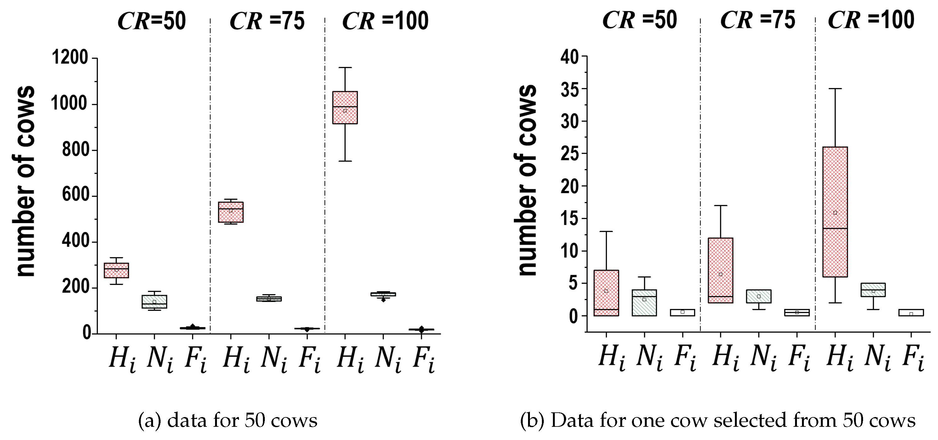
To evaluate the advantages of selection under the proposed algorithm, simulations of configuration were conducted while varying . The simulations employed 30 distinct initial distributions of 50 cows, with configured to 50, 75, and 100 units. After configuration in individual simulations, the numbers of cows in and for each cow were recorded and summed. Additionally, one cow was selected to compare its behavior with that of the entire 50-cow herd. The statistical results are shown in Figure 29, where error bars indicate 95% confidence intervals and boxes represent the 25–75% interquartile range. As expected from communication properties, the number of cows in increased with the expansion of . In contrast, the size of remained largely stable regardless of . Similarly, the selection exhibited a consistent trend regardless of . Consequently, these findings demonstrate that selection is robust to variations in , as each tag identifies neighbors with higher connectivity using local distribution information.
6. Conclusions
In this study, we focused on the monitoring of herd patterns and inter-cow relationships by using relative-communication distances and neighbor-centered networks. We proposed a local network generation algorithm using a two-layer communication range, and validated it through extensive experiments with cows equipped with wireless sensor tags. The proposed algorithm enabled the configuration of star networks among selected neighbors, and by combining local networks, a global partially connected mesh network self-organized. By incorporating signal strength relative to distances, the network adapted to changes caused by cow movements. Field experiments demonstrated that the friend selection function reflects both affiliative interactions and social isolation in cows, whereas simulations confirmed the feasibility of generating and reconfiguring networks within large herds. The proposed algorithm allows monitoring of an affinity behavior and isolation status in grazing environments, potentially reducing labor for livestock management and improving productivity.
Author Contributions
Conceptualization, G.Lee; methodology, G.Lee, K.Okabe, and F.Sugino; software, T.Yamane, K.Okabe, and Y.Kyung; validation, G.Lee, F.Sugino, and Y.Kyung; formal analysis, T.Yamane, K.Okabe, and F.Sugino; investigation, G.Lee and K.Okabe; resources, G.Lee and F.Sugino; data curation, G.Lee and Y.Kyung; writing—original draft preparation, G.Lee and K.Okabe; writing—review and editing, G.Lee, T.Yamane, and Y.Kyun; visualization, G.Lee and T.Yamane; supervision, G.Lee and F.Sugino; project administration, G.Lee; funding acquisition, G.Lee and F.Sugino. All authors have read and agreed to the published version of the manuscript.
Funding
This research received no external funding.
Institutional Review Board Statement
All experiments were conducted in compliance with the protocol which was reviewed by the Institutional Animal Care and Use Committee and approved by the President of the University of Miyazaki (Permission Number: 2021-026-2).
Informed Consent Statement
Not applicable.
Data Availability Statement
Data are contained within the article.
Acknowledgments
Special thanks to Seiya Sakaguchi and Ryoichi Aizawa for data analysis and technical assistance. Their extraordinary contributions have greatly improved the quality of this thesis paper.
Conflicts of Interest
The authors declare no conflicts of interest.
Abbreviations
The following abbreviations are used in this manuscript:
| communication range of each cow | |
| specific range determined by radio wave strength where | |
| mutual friends within | |
| split into multiple local networks | |
| unified single network | |
| isolated state |
References
- Dawkins, M.S. Smart farming and artificial intelligence (AI): How can we ensure that animal welfare is a priority? Applied Animal Behaviour Science 2025, 283, 106519. [Google Scholar] [CrossRef]
- Yin, M.; Ma, R.; Luo, H.; Li, J.; Zhao, Q.; Zhang, M. Non-contact sensing technology enables precision livestock farming in smart farms. Computers and Electronics in Agriculture 2023, 212, 108171. [Google Scholar] [CrossRef]
- Lee, G.; Ogata, K.; Kawasue, K.; Sakamoto, S.; Ieiri, S. Identifying-and-counting based monitoring scheme for pigs by integrating BLE tags and WBLCX antennas. Computers and Electronics in Agriculture 2022, 198, 107070. [Google Scholar] [CrossRef]
- Wang, R.; Li, Y.; Tian, F.; Liu, Y.; Wang, Z.; Yuan, C.; Lu, X. Estrus detection in dairy cows using advanced object tracking and behavioral analysis technologies. Computers and Electronics in Agriculture 2025, 235, 110331. [Google Scholar] [CrossRef]
- Merkelytė, I.; Siukscius, A.; Nainiene, R. The role of sensor technologies in estrus detection in beef cattle: A review of current applications. Animals 2025, 15, 2313. [Google Scholar] [CrossRef] [PubMed]
- Bretzinger, L.F.; Hölper, M.; Tippenhauer, C.M.; Plenio, J.-L.; Madureira, A.; Heuwieser, W.; Borchardt, S. Evaluation of four different automated activity monitoring systems to identify anovulatory cows in early lactation. Animals 2024, 14, 3145. [Google Scholar] [CrossRef] [PubMed]
- Johansen, F.P.; Buijs, S.; Arnott, G. Providing concentrate feed outside of the milking robot increases feed intake in dairy cows without reducing motivation to visit the robot. Animal 2025, 19, 101459. [Google Scholar] [CrossRef]
- Romano, E.; Brambilla, M.; Cutini, M.; Giovinazzo, S.; Lazzari, A.; Calcante, A.; Tangorra, F.M.; Rossi, P.; Motta, A.; Bisaglia, C.; et al. Increased cattle feeding precision from automatic feeding systems: Considerations on technology spread and farm level perceived advantages in Italy. Animals 2023, 13, 3382. [Google Scholar] [CrossRef]
- Han, Y.; Wu, J.; Zhang, H.; Cai, M.; Sun, Y.; Li, B.; Feng, X.; Hao, J.; Wang, H. Beef cattle abnormal behaviour recognition based on dual-branch frequency channel temporal excitation and aggregation. Biosystems Engineering 2024, 241, 28–42. [Google Scholar] [CrossRef]
- Jurkovich, V.; Hejel, P.; Kovács, L. A review of the effects of stress on dairy cattle behaviour. Animals 2024, 14, 2038. [Google Scholar] [CrossRef]
- Arablouei, R.; Bishop-Hurley, G.J.; Bagnall, N.; Ingham, A. Cattle behavior recognition from accelerometer data: Leveraging in-situ cross-device model learning. Computers and Electronics in Agriculture 2024, 227, 109546. [Google Scholar] [CrossRef]
- Ding, L.; Lv, Y.; Jiang, R.; Zhao, W.; Li, Q.; Yang, B.; Yu, L.; Ma, W.; Gao, R.; Yu, Q. Predicting the feed intake of cattle based on jaw movement using a triaxial zccelerometer. Agriculture 2022, 12, 899. [Google Scholar] [CrossRef]
- Nogoy, K.M.C.; Chon, S.-i.; Park, J.-h.; Sivamani, S.; Lee, D.-H.; Choi, S.H. High precision classification of resting and eating behaviors of cattle by using a collar-fitted triaxial accelerometer sensor. Sensors 2022, 22, 5961. [Google Scholar] [CrossRef]
- Benaissa, S.; Tuyttens, F.A.M.; Plets, D.; Martens, L.; Vandaele, L.; Joseph, W.; Sonck, B. Improved cattle behaviour monitoring by combining Ultra-Wideband location and accelerometer data. Animal 2023, 17, 100730. [Google Scholar] [CrossRef]
- Ojo, M.O.; Viola, I.; Baratta, M.; Giordano, S. Practical experiences of a smart livestock location monitoring system leveraging GNSS, LoRaWAN and cloud services. Sensors 2022, 22, 273. [Google Scholar] [CrossRef] [PubMed]
- Bloch, V.; Pastell, M. Monitoring of cow location in a barn by an open-source, low-cost, low-energy bluetooth tag system. Sensors 2020, 20, 3841. [Google Scholar] [CrossRef]
- Wang, Y.; Perea, A.; Cao, H.; Bakir, M.; Utsumi, S. A two-stage machine learning approach for calving detection in rangeland cattle. Agriculture 2025, 15, 1434. [Google Scholar] [CrossRef]
- Liao, M.; Morota, G.; Bi, Y.; Cockrum, R.R. Predicting dairy calf body weight from depth images using deep learning (YOLOv8) and threshold segmentation with cross-validation and longitudinal analysis. Animals 2025, 15, 868. [Google Scholar] [CrossRef] [PubMed]
- Ferreira, C.; Todorovic, M.; Sugrue, P.; Teixeira, S.; Galvin, P. Review: Emerging sensors and instrumentation systems for bovine health monitoring. Animal 2025, 19, 101527. [Google Scholar] [CrossRef]
- Galik, R.; Bod’o, Š.; Lüttmerding, A.; Knížková, I.; Kunc, P. Tracking differences in cow temperature related to environmental factors. Applied. Science 2024, 14, 7205. [Google Scholar] [CrossRef]
- Li, J.; Ling, M.; Fu, B.; et al. UAV based smart grazing: a prototype of space-air-ground integrated grazing IoT networks in Qinghai-Tibet plateau. Discover Internet of Things 2025, 5. [Google Scholar] [CrossRef]
- Casas, R.; Hermosa, A.; Marco, Á.; Blanco, T.; Zarazaga-Soria, F.J. Real-time extensive livestock monitoring using LPWAN smart wearable and infrastructure. Applied Science 2021, 11, 1240. [Google Scholar] [CrossRef]
- Cabezas, J.; Yubero, R.; Visitación, B.; Navarro-García, J.; Algar, M.J.; Cano, E.L.; Ortega, F. Analysis of accelerometer and GPS data for cattle behaviour identification and anomalous events detection. Entropy 2022, 24, 336. [Google Scholar] [CrossRef] [PubMed]
- Rivero, M.J.; Grau-Campanario, P.; Mullan, S.; Held, S.D.E.; Stokes, J.E.; Lee, M.R.F.; Cardenas, L.M. Factors affecting site use preference of grazing cattle studied from 2000 to 2020 through GPS tracking: A review. Sensors 2021, 21, 2696. [Google Scholar] [CrossRef]
Figure 1.
Concept of monitoring application to a herd of pastured cows.
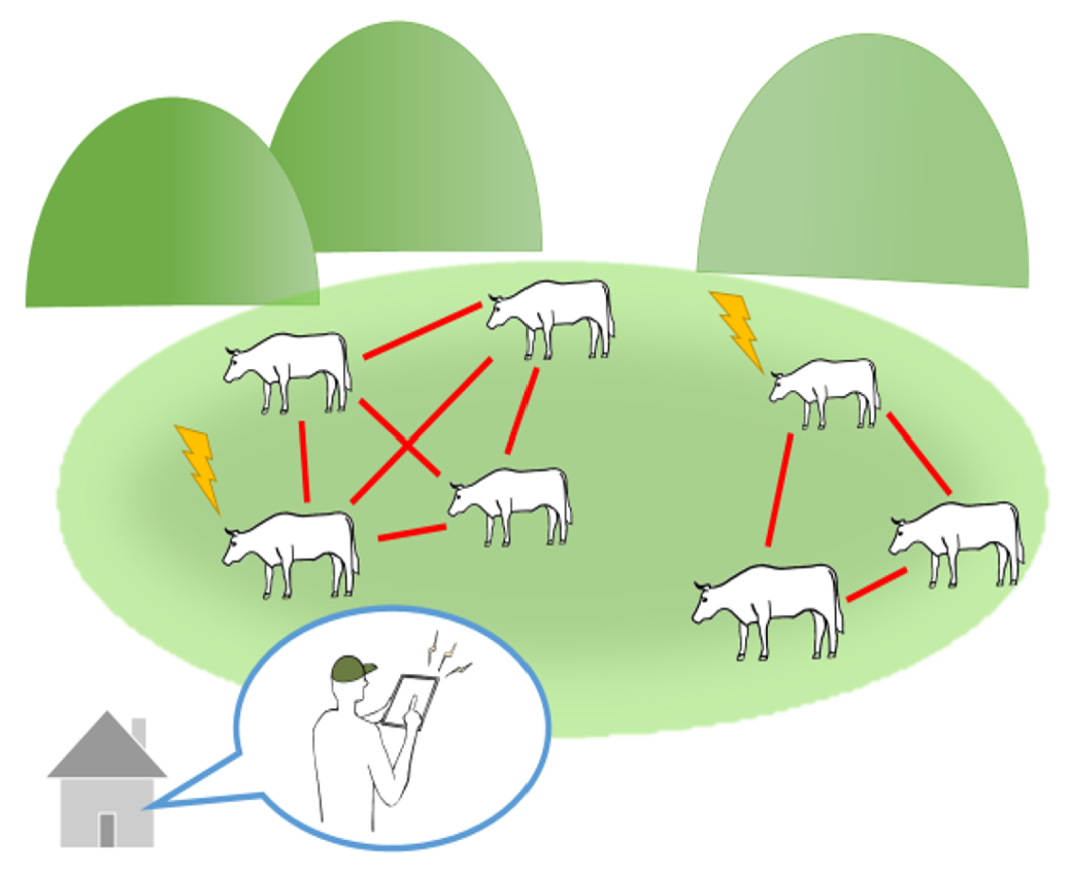
Figure 2.
Definitions and notations.
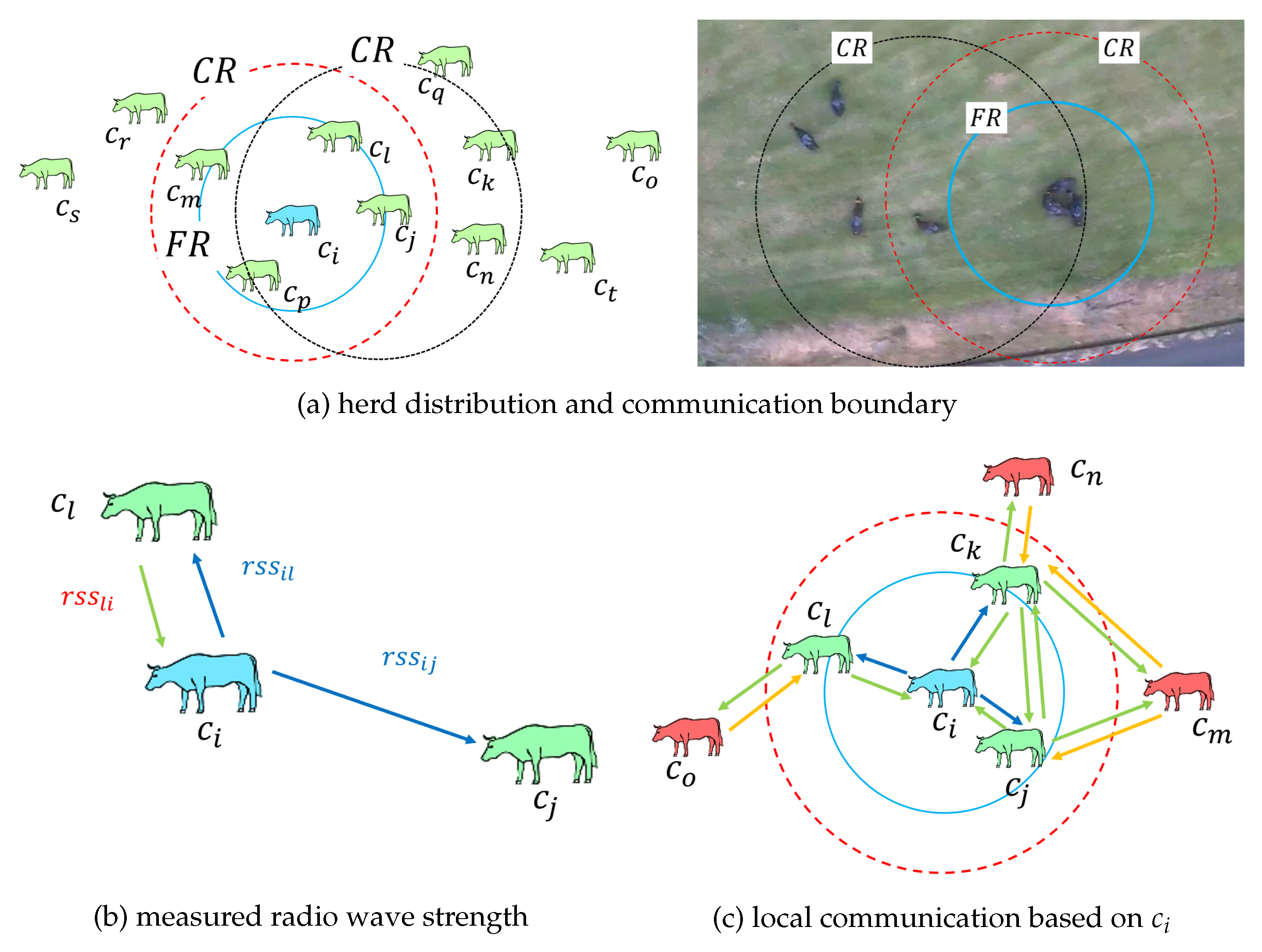
Figure 3.
Three message types used for communication.
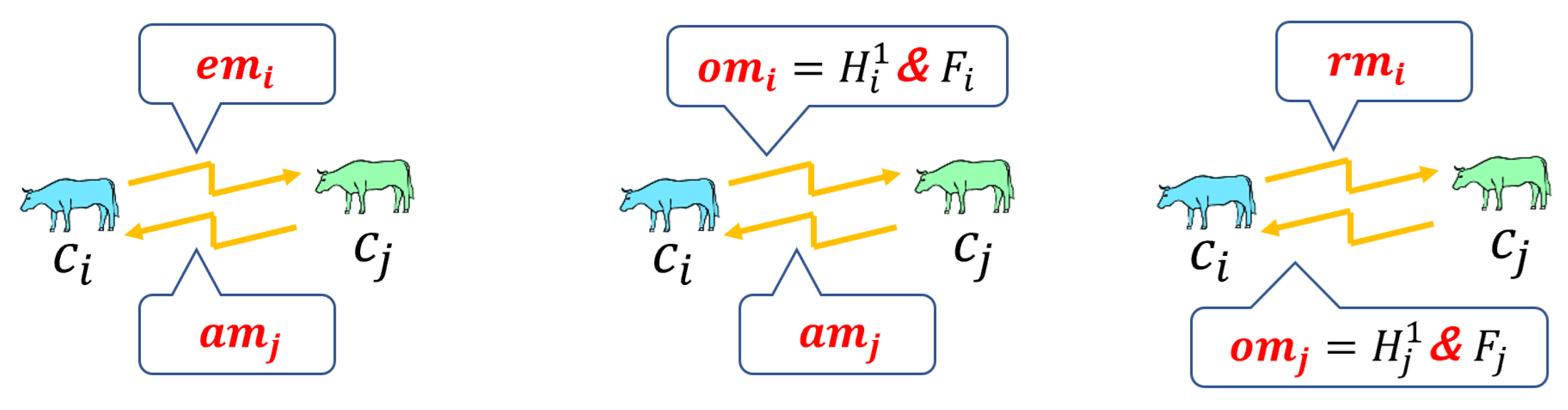
Figure 4.
Collective behaviors of cows.
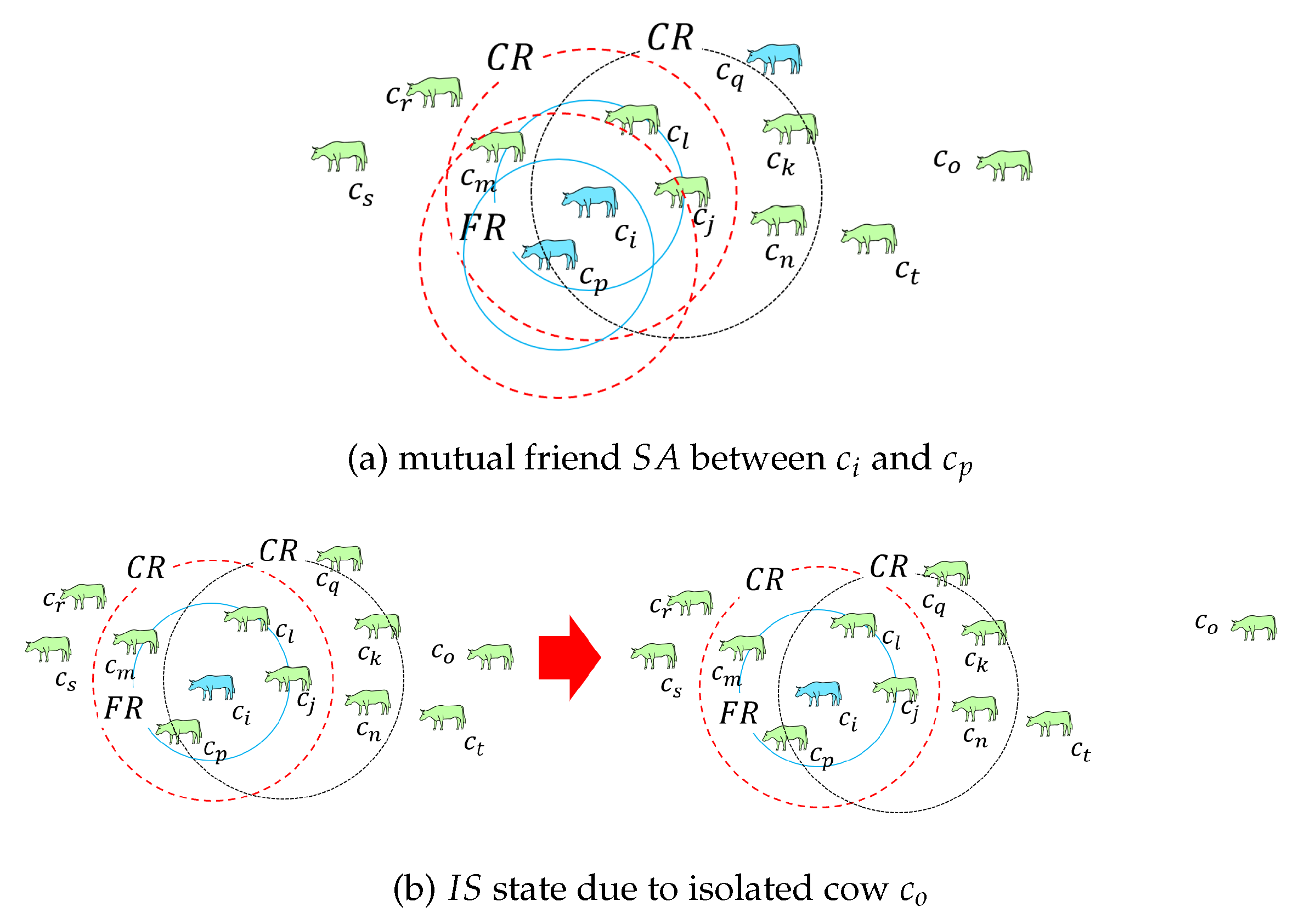
Figure 5.
Schematic flow of monitoring algorithm based on .
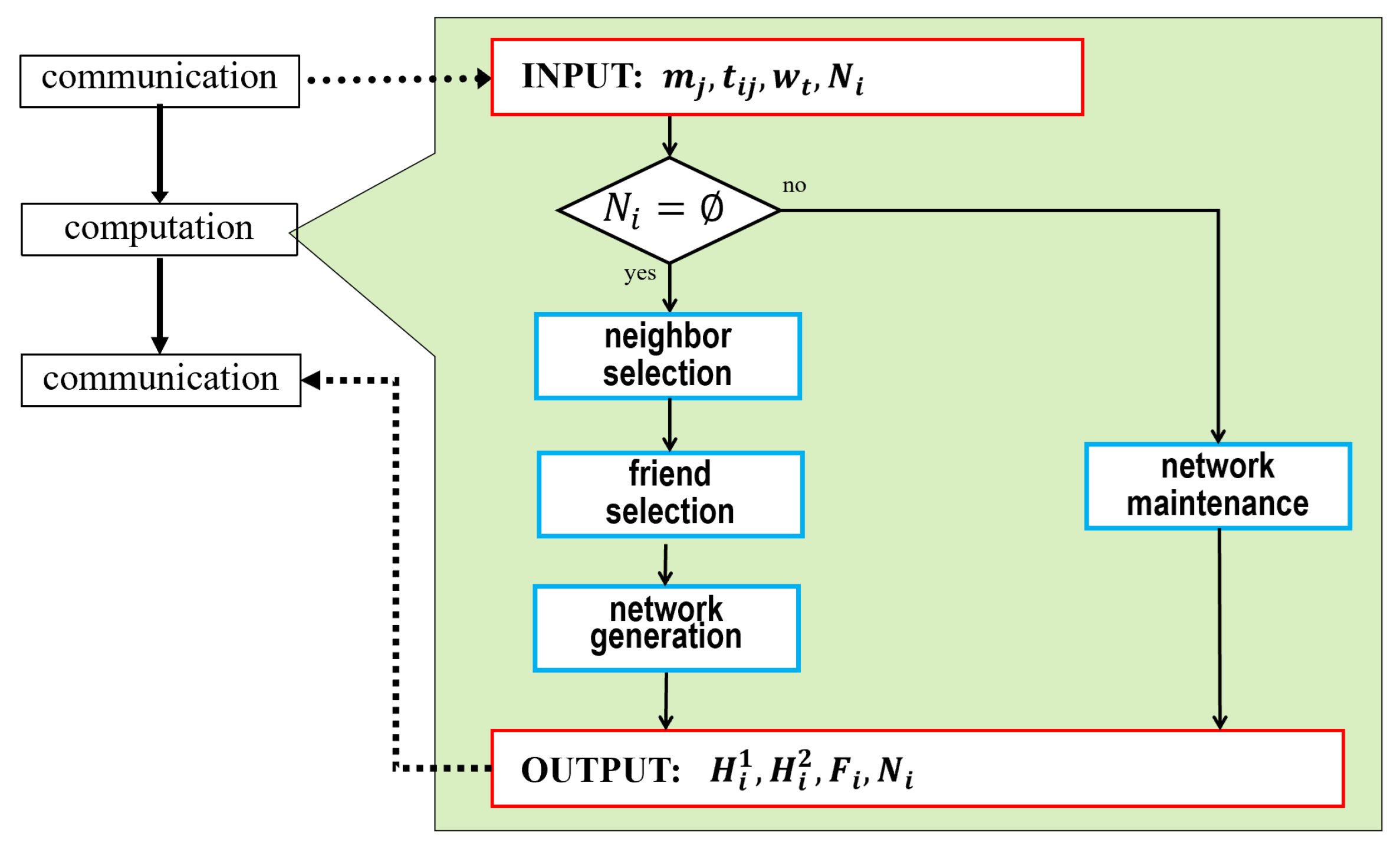
Figure 6.
Illustration of acquisition (left: cow distribution; right: corresponding table ).
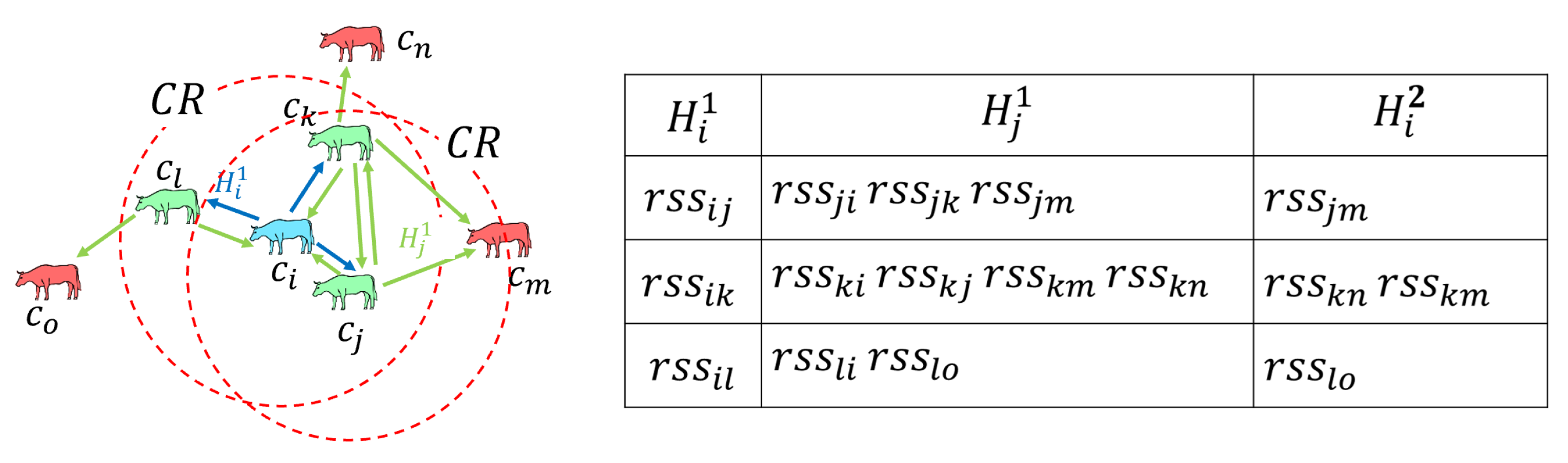
Figure 7.
and computation process.
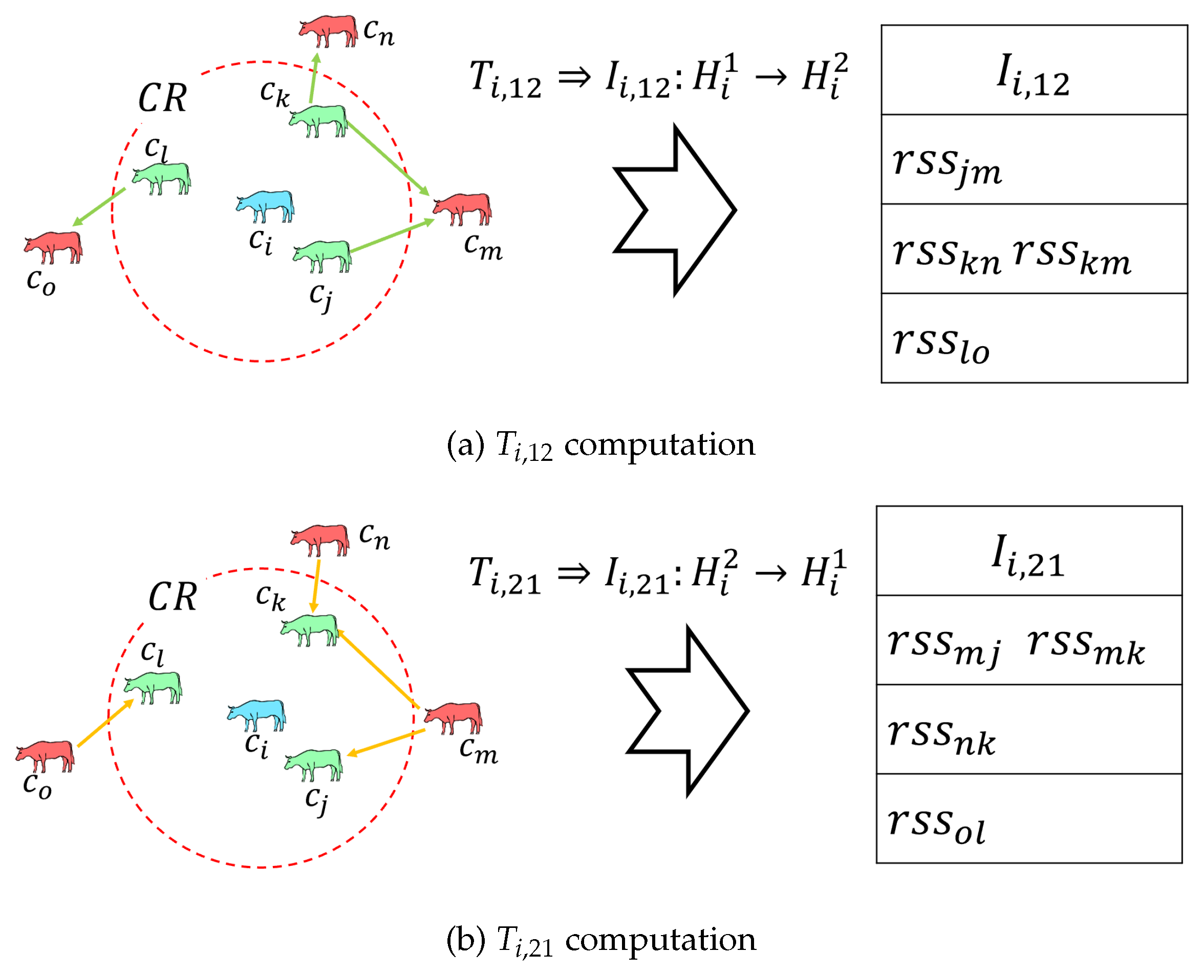
Figure 8.
Illustration of calculation (left: cow distribution; right: calculation table).
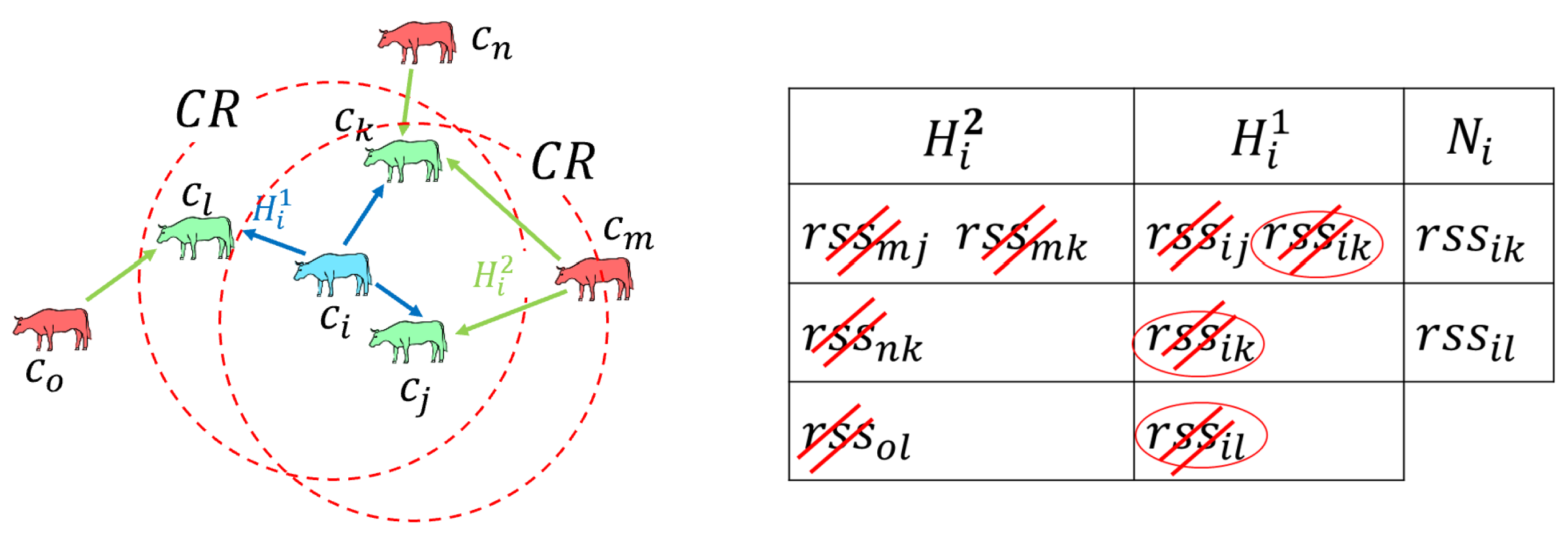
Figure 9.
Illustration of calculation (left: cow distribution; right: calculation table).
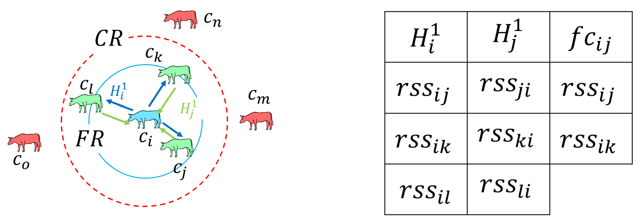
Figure 10.
Illustration of calculation (left: cow distribution; right: calculation table).
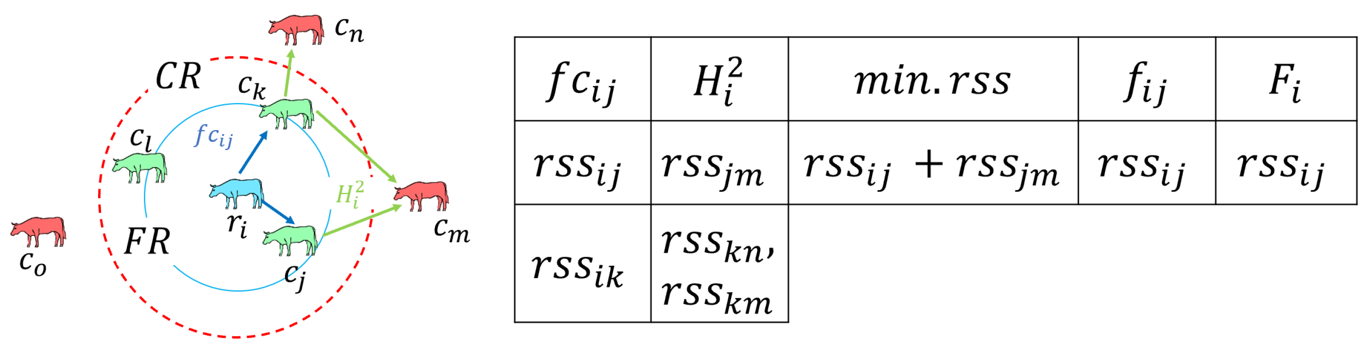
Figure 11.
Illustration of generation.
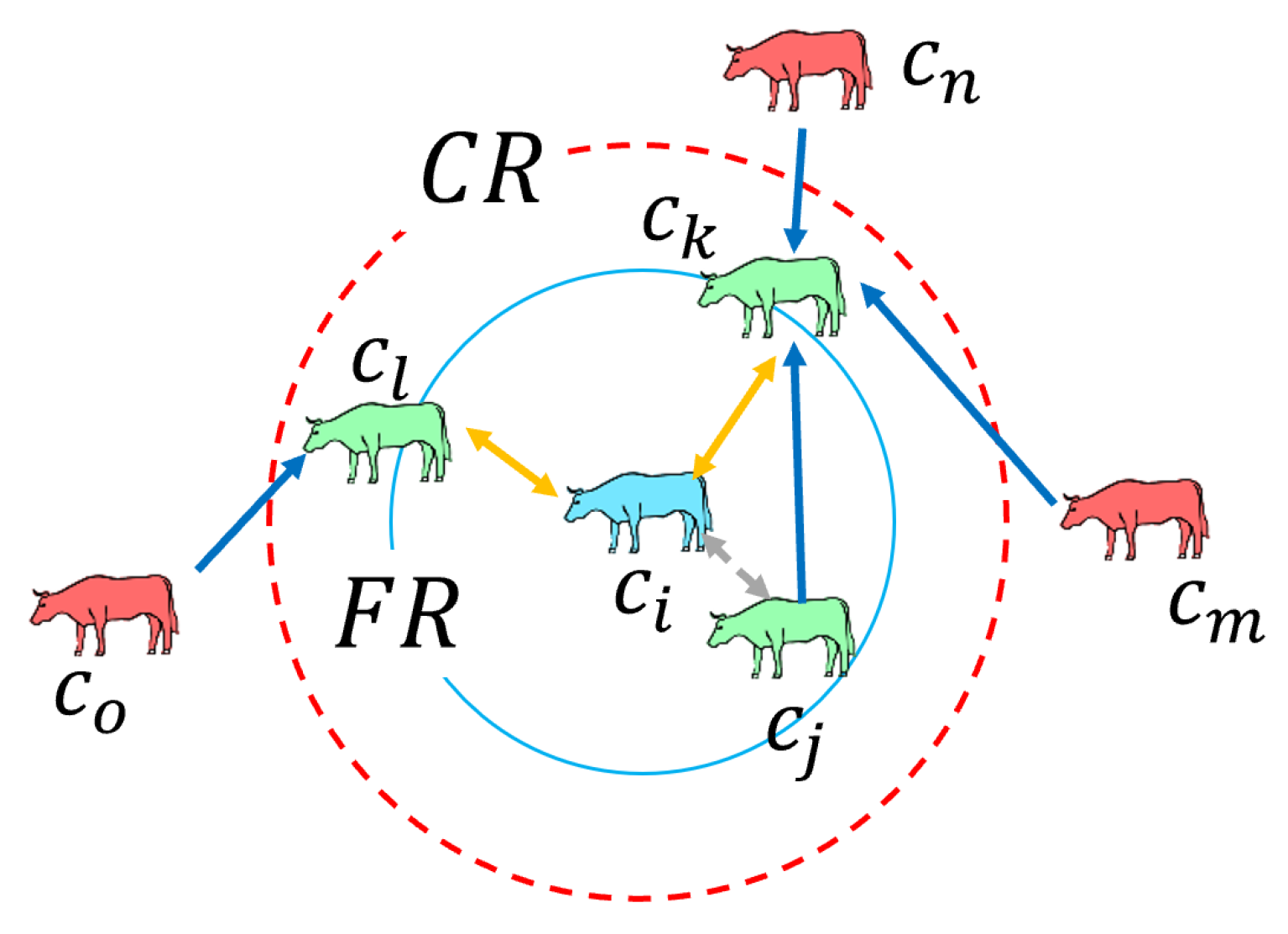
Figure 12.
Variations in communication conditions with cow movements.
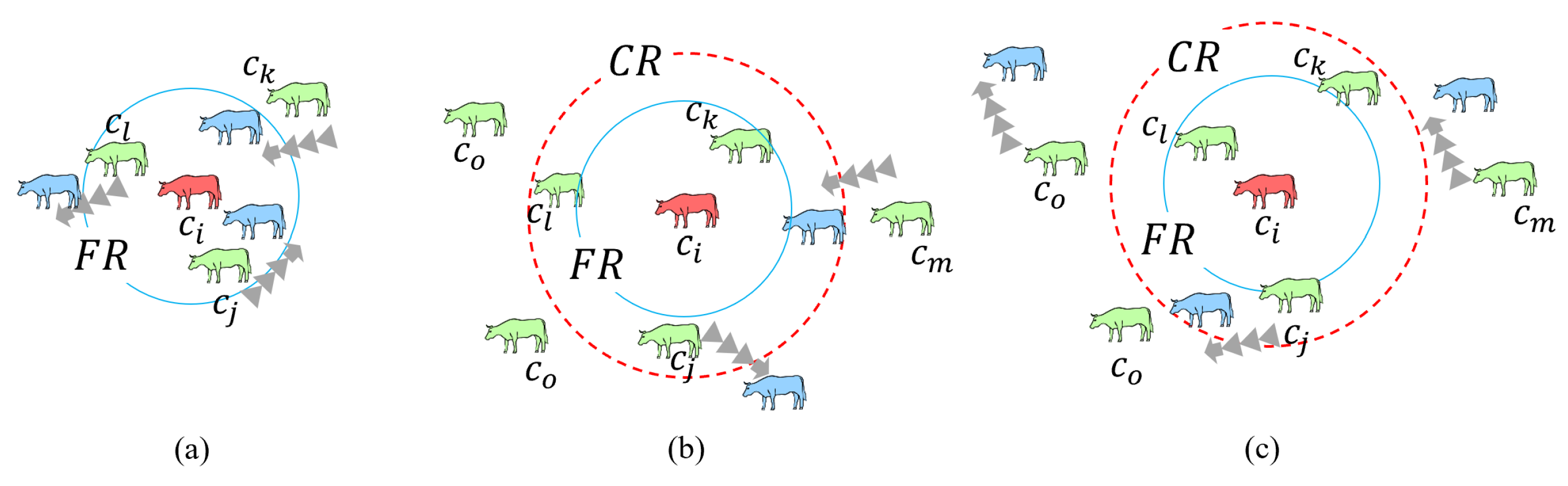
Figure 13.
Hardware configuration of a wireless sensor and a server tags.
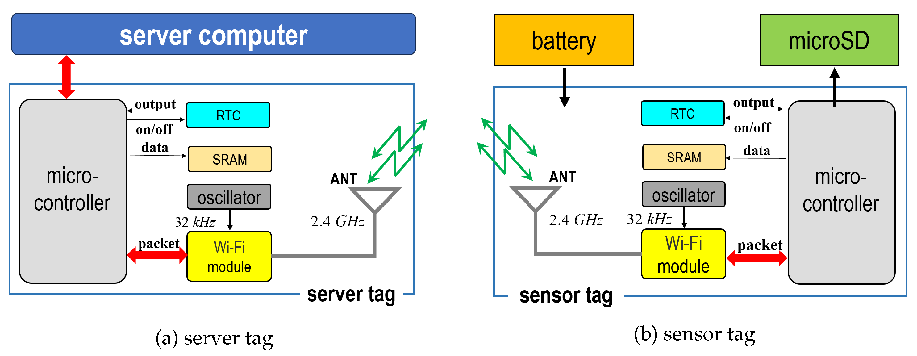
Figure 14.
Structure of packets used for communication.
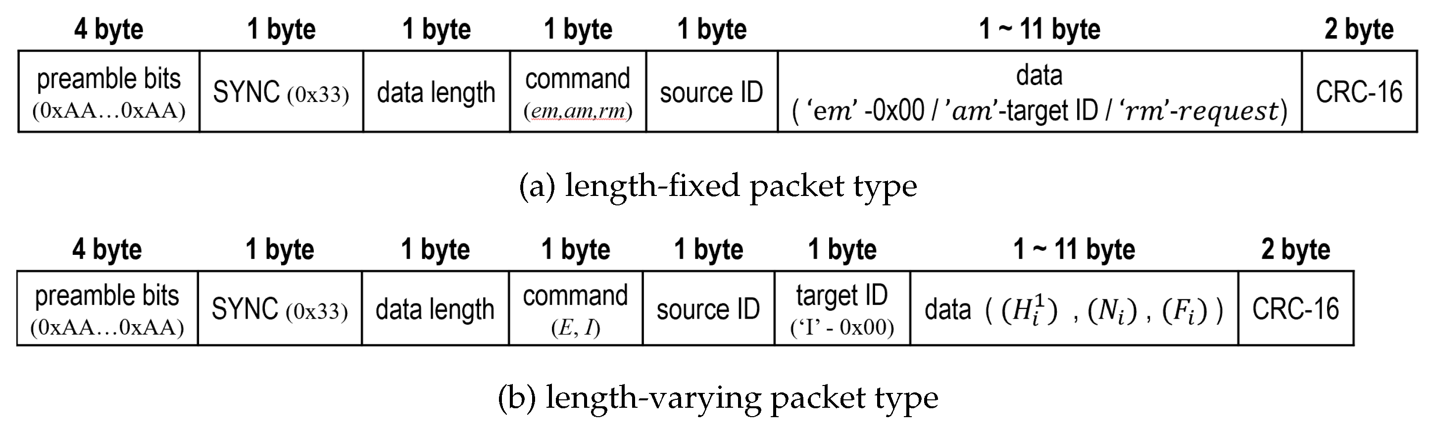
Figure 15.
Specification and layout of electronic module.
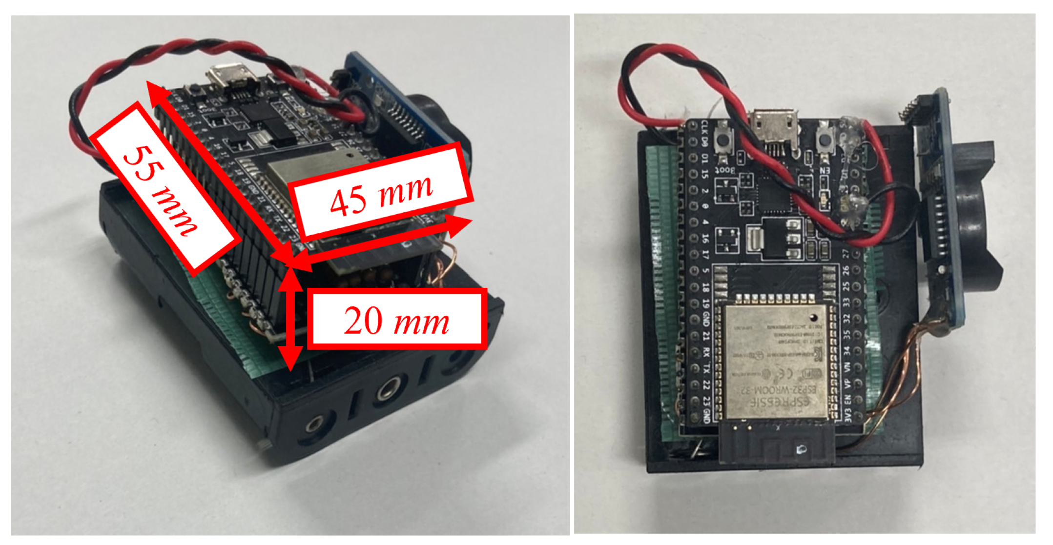
Figure 16.
Wireless sensor tag mounted on frame unit.
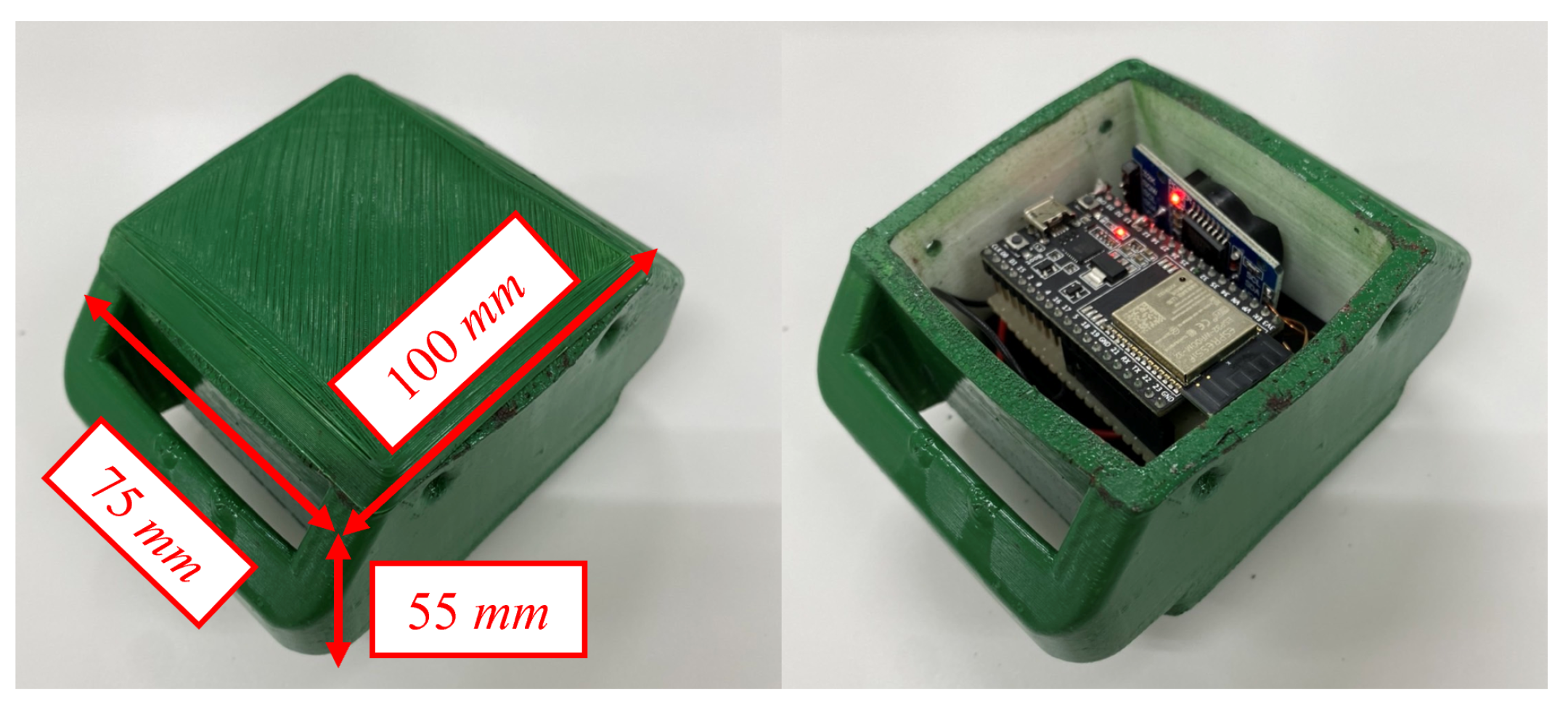
Figure 17.
Measurement results for variation in signal strength over distance.
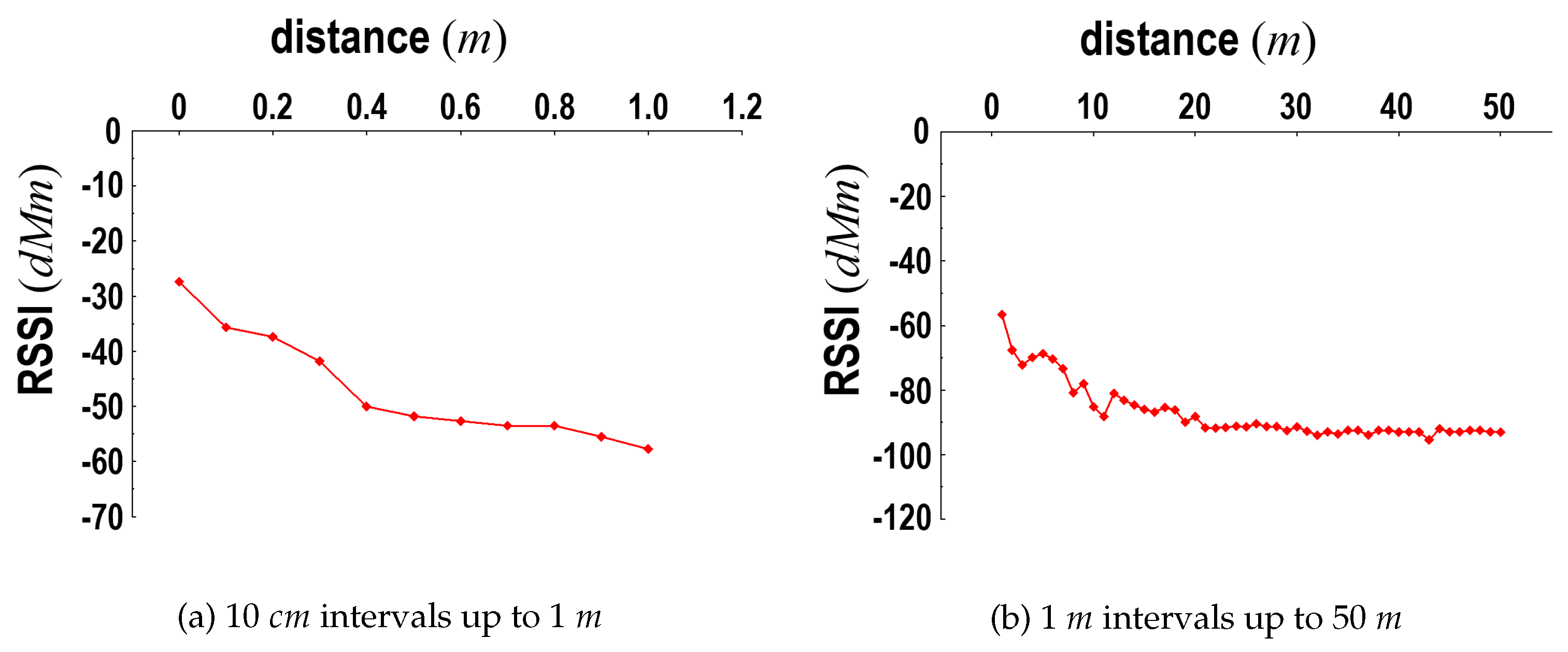
Figure 18.
Experimental environment and sensor tag mounted on cows.
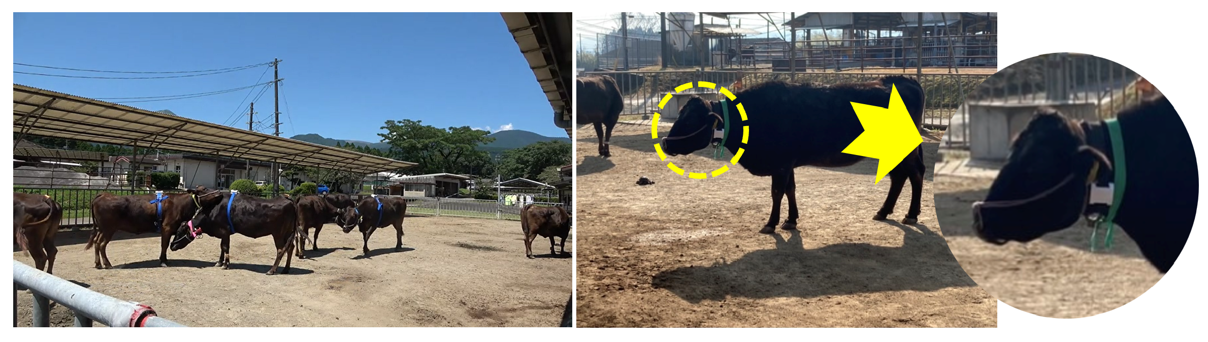
Figure 19.
Experimental results for network generation with respect to server tag according to movements of five sensor tags.
Figure 19.
Experimental results for network generation with respect to server tag according to movements of five sensor tags.
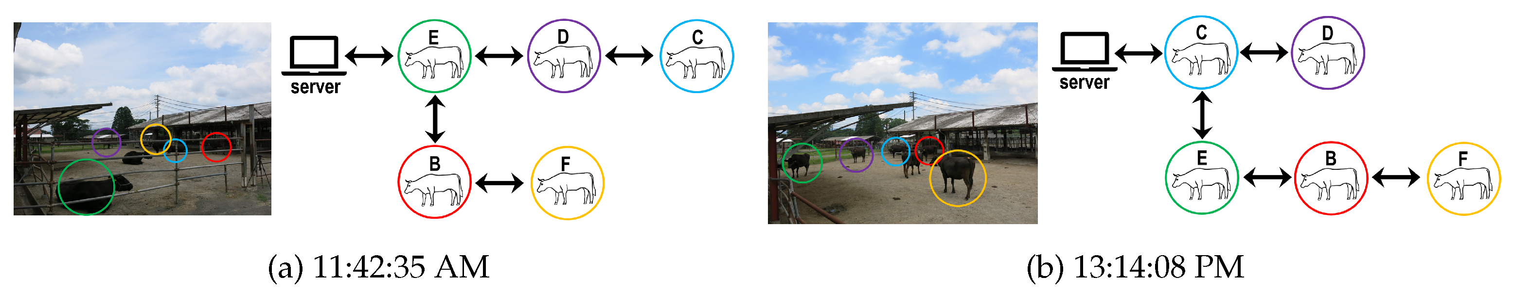
Figure 20.
Experimental scene for network configuration with respect to green circled cow.
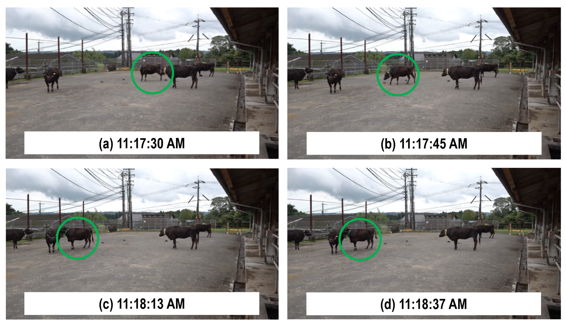
Figure 21.
Experimental results for changes in network configuration according to movements of green-circled cow.
Figure 21.
Experimental results for changes in network configuration according to movements of green-circled cow.
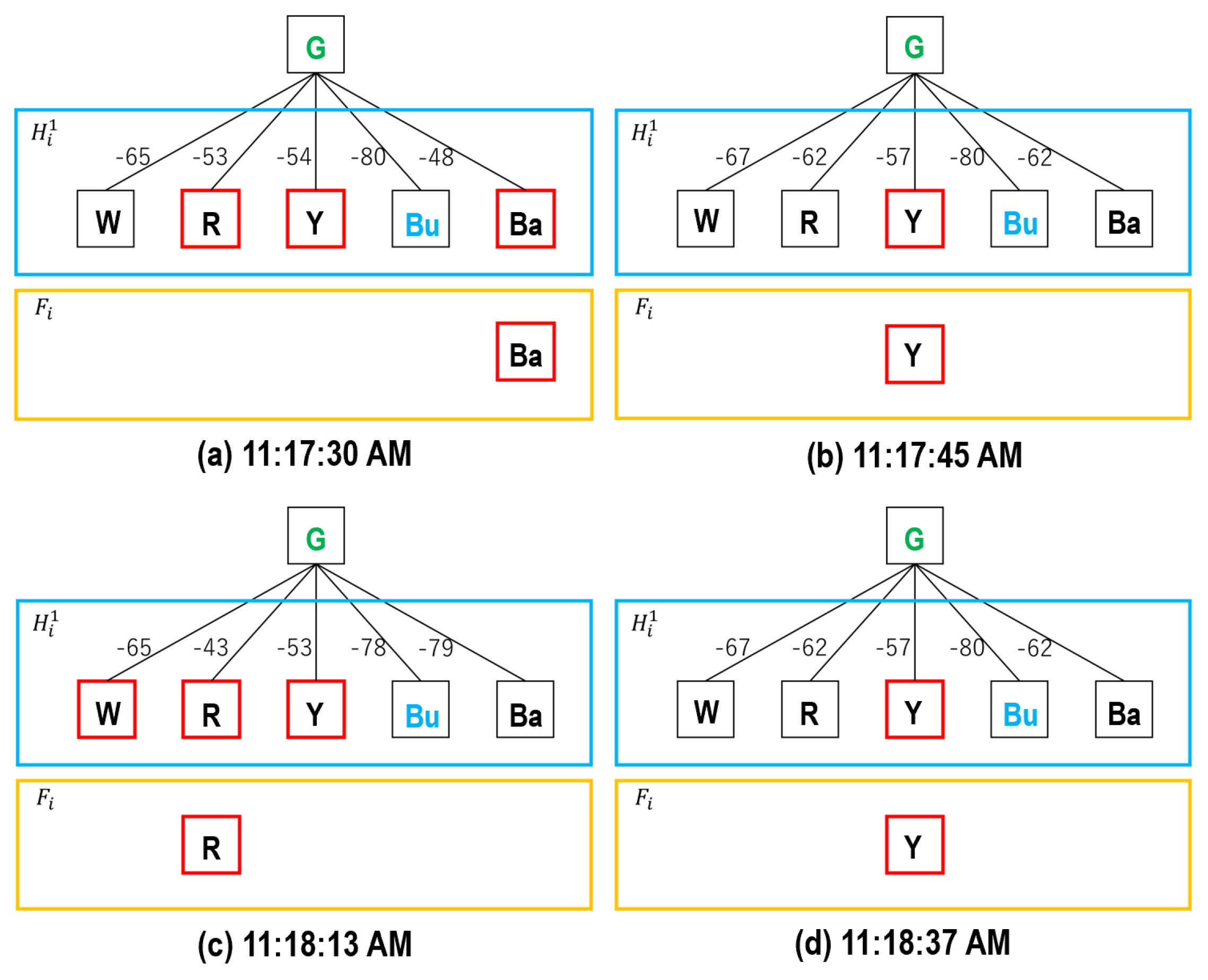
Figure 22.
Experimental scene for network configuration observed when cows gathered at feeder.
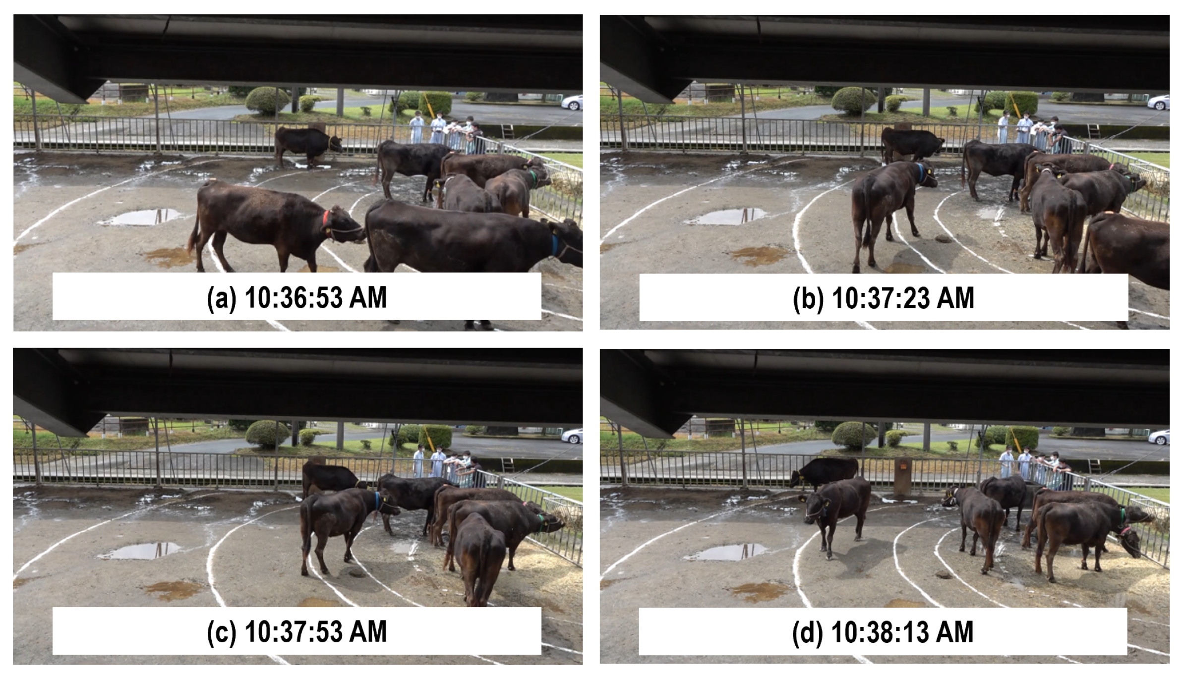
Figure 23.
Distance-dependent variation in signal strength from feeder.
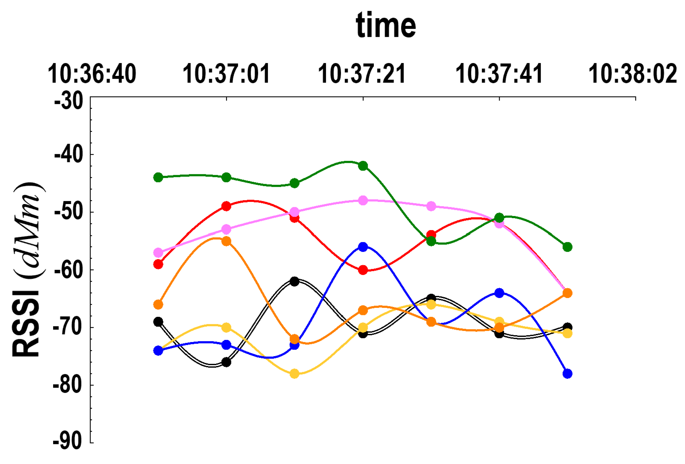
Figure 24.
Experimental scene for network configuration observed when cows entered cowshed.
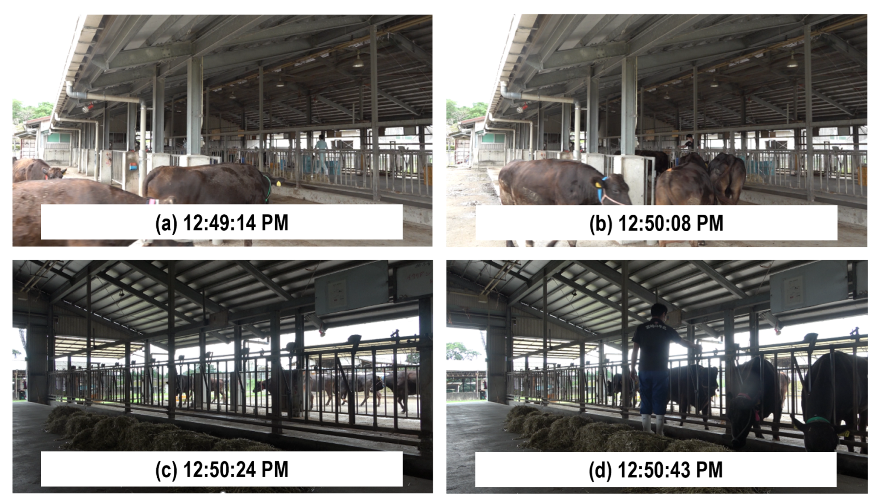
Figure 25.
Distance-dependent variation in signal strength from entrance.
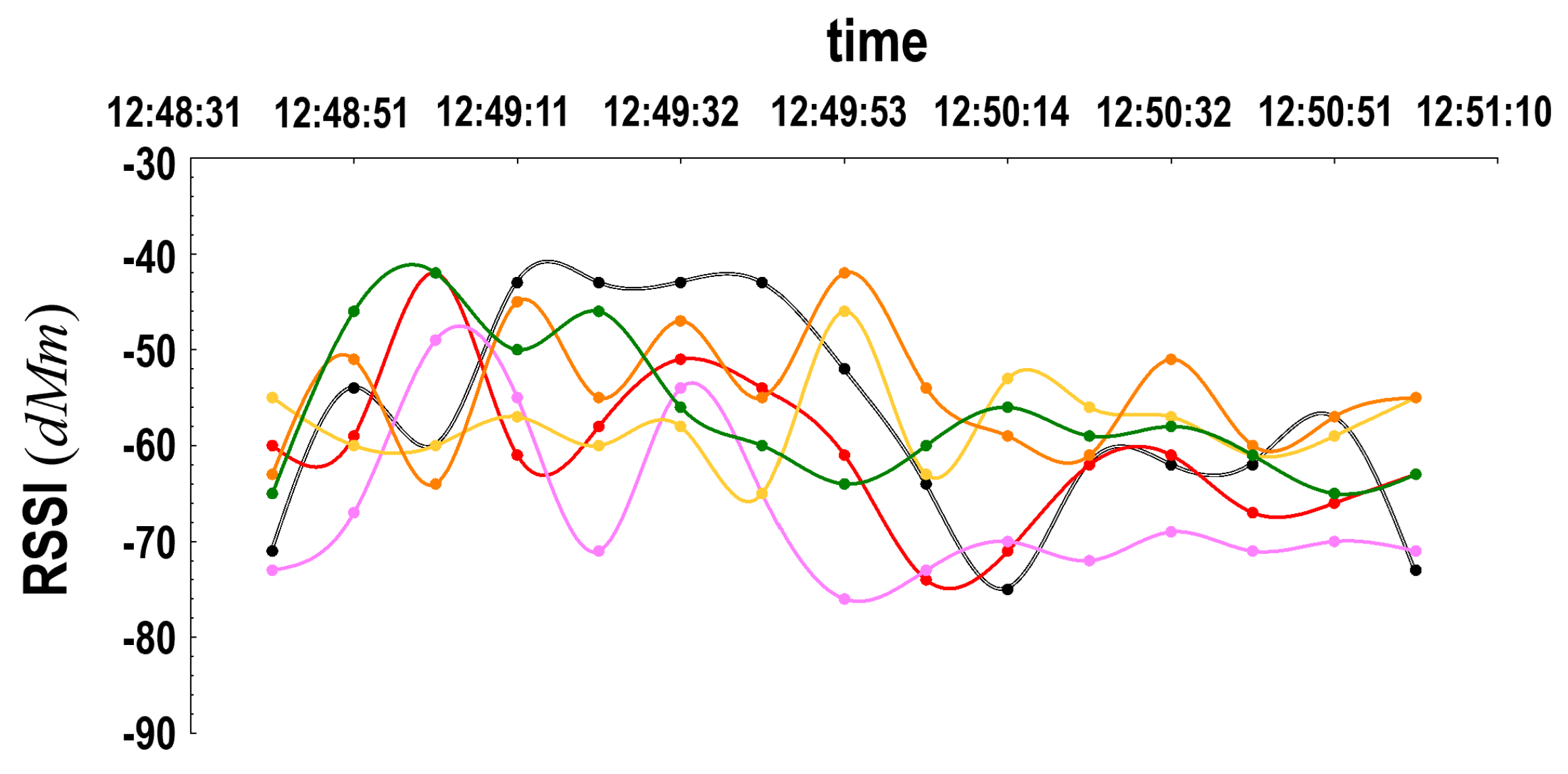
Figure 26.
Experimental result for group behaviors of grazing cows and corresponding network configuration.
Figure 26.
Experimental result for group behaviors of grazing cows and corresponding network configuration.
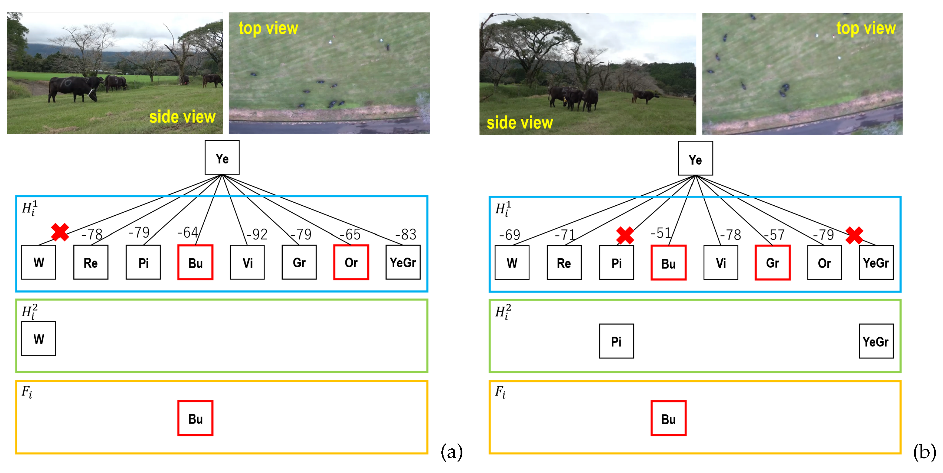
Figure 27.
Variations in signal strength when two cows leaving herd.
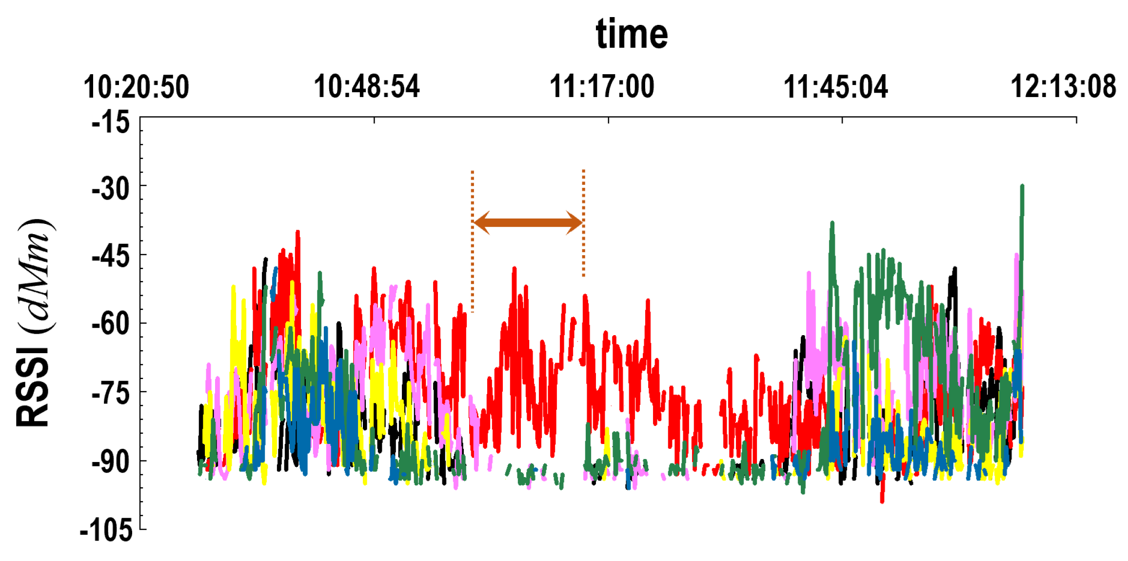
Figure 28.
Simulation results for network configuration based on movements of five cows.
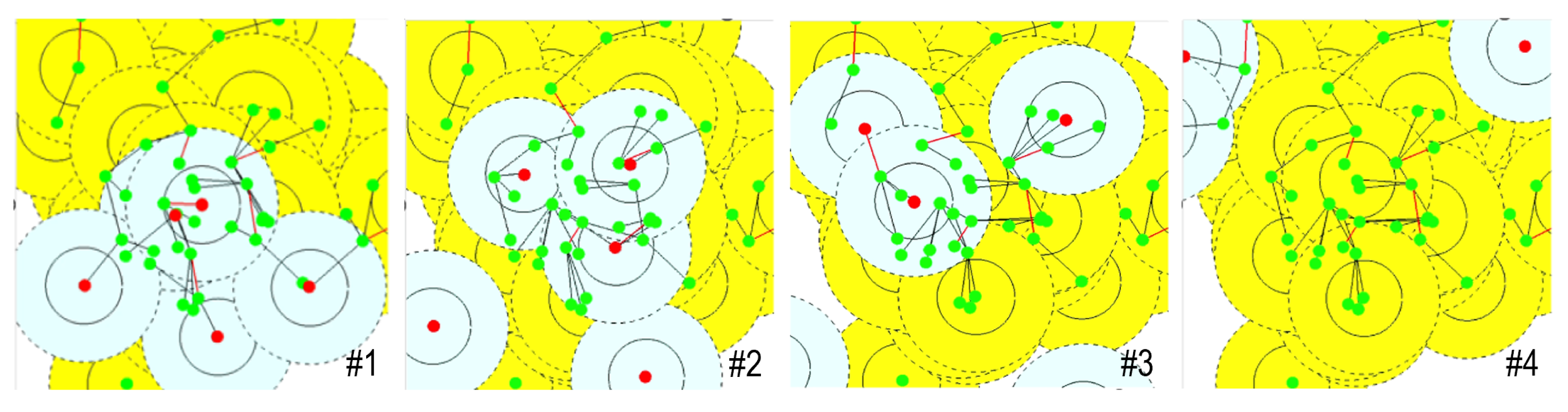
Figure 29.
Simulation results for the number of cows in , , and with varying .
Disclaimer/Publisher’s Note: The statements, opinions and data contained in all publications are solely those of the individual author(s) and contributor(s) and not of MDPI and/or the editor(s). MDPI and/or the editor(s) disclaim responsibility for any injury to people or property resulting from any ideas, methods, instructions or products referred to in the content. |
© 2025 by the authors. Licensee MDPI, Basel, Switzerland. This article is an open access article distributed under the terms and conditions of the Creative Commons Attribution (CC BY) license (http://creativecommons.org/licenses/by/4.0/).
Copyright: This open access article is published under a Creative Commons CC BY 4.0 license, which permit the free download, distribution, and reuse, provided that the author and preprint are cited in any reuse.


