
Submitted:
30 October 2025
Posted:
31 October 2025
You are already at the latest version
Abstract
Quantitative Polymerase Chain Reaction (qPCR) is a very sensitive method to determine small amounts of DNA or RNA in experimental, environmental, veterinary, forensic and clinical samples. Despite efforts from the qPCR community to address qPCR variability by recommending standardization of reporting of all steps of a qPCR experiment, most reported qPCR results are still grossly biased. The first part of this paper describes two decades of efforts to remedy this situation by promoting so-called efficiency-corrected qPCR data analysis. Although such analysis leads to less variable qPCR results, the outcome, fluorescence at cycle zero, is difficult to grasp. In the second part, we outline how qPCR analysis can result in Ncopy, the number of copies of the target at the start of the reaction. This newly developed theoretical approach determines Ncopy using the characteristics of the amplification curve and the known concentrations of all reaction components. By including these reaction-mix characteristics in the analysis, this Ncopy is assay, machine and laboratory independent and thus allows direct worldwide comparisons. Moreover, Ncopy provides a very intuitive and easy to interpret absolute quantitative result.
Keywords:
qPCR
; PCR efficiency
; amplification curves
; absolute quantification
; baseline correction
; quantification threshold
; reaction components
; limiting conditions
1. Introduction
Quantitative Polymerase Chain Reaction (qPCR) is worldwide the method of choice to determine the presence of small amounts of DNA or RNA reflecting the presence of pathogens or organisms in samples collected in clinical, environmental and forensic research or the expression level of genes in samples collected in basic and experimental research [1,2]. qPCR is considered to be a very sensitive and precise method to determine the number of copies of a target of interest in a given sample. However, reproducibility of qPCR results has been the subject of discussion for decades [3,4]. Despite the efforts to standardize the reporting of all steps of a qPCR experiment [2,5,6], crucial steps in the analysis of qPCR data are still widely ignored and therefore grossly biased qPCR results are accepted by reviewers and journals [7,8,9]. The first part of this paper describes our two decades of efforts to remedy part of this situation by promoting so-called efficiency-corrected qPCR data analysis [10,11,12]. In the second part, we will outline a newly developed approach using the characteristics of the amplification curve and the knowledge about the concentrations of reaction components to determine the actual number of target copies at the start of a reaction.
2. The qPCR Basics
2.1. PCR Kinetics
Each reaction in a PCR run comprises of the sample to be measured, a heat-stable DNA polymerase, a reaction buffer, nucleotides, primers and a fluorescent DNA binding dye or probe [13]. The pair of forward and reverse primer is designed such that it specifically flanks the so-called amplicon: the target of interest (toi) region in the DNA. During a qPCR run the reaction mixture is repeatedly heated and cooled in so-called amplification cycles. One amplification cycle comprises of heating the reaction to 95°C to denature the DNA into single strands, cooling to the annealing temperature, which is chosen such that the primers specifically and uniquely bind around the target sequences, followed by heating to 72°C at which the heat-stable DNA polymerase synthesizes the complementary DNA strands starting at the forward or reverse primer resulting in two double strand amplicons. In clinical studies, often a 2-step PCR reaction is done, in which both the annealing of the primers and subsequent DNA synthesis are executed at the same temperature [14]. In both setups, the exponential accumulation of the amplicon during the PCR run is described by the kinetic equation NC=N0EC [11]. In words, the number of amplicons after a given amplification cycle (NC) is equal to the number of copies of the target at the start of the PCR (N0) times the efficiency of the amplification reaction (E) to the power the given cycle (C). The amplification efficiency is thus defined as the fold-increase per cycle, and has a value between 1 and 2, where 2 is a 100% efficient reaction in which in each cycle the number of amplicons is doubled. In this paper the symbol N0 will also be referred to as the target quantity.
2.2. Fluorescence Monitoring During the PCR
Because it is impossible to directly measure the number of target molecules at the start of the PCR, the number of amplicons at every cycle of a reaction is monitored indirectly by measuring the fluorescence of a dye or probe [15,16]. As a consequence, a qPCR machine reports fluorescence values (F), that are corrected for system background fluorescence, which is the fluorescence that is independent of the monitoring chemistry and cycling [17]. The kinetic equation of PCR should actually be written as FC = F0EC. These fluorescence values can be used to plot the amplification curve. In every day practice, the exponential phase of a PCR is only a limited number of cycles in the amplification curve (Figure 1a,b). This exponential phase is preceded by a ground phase, in which the amplicon is exponentially amplified but the fluorescence resulting from monitoring these amplicons is insufficient to exceed the baseline fluorescence. This baseline fluorescence is defined as the fluorescence of the PCR monitoring dye or probe but is independent of the amplification. The exponential phase ends when one of the reaction components becomes limiting and consequently the observed PCR efficiency starts to decrease. This decrease in PCR efficiency is reflected in the amplification curve as the transition phase towards the plateau phase. In the latter phase the fluorescence remains constant.
2.3. Common Analysis of qPCR Data
Analysis of qPCR data commonly consists of the following basic steps: 1) subtraction of baseline fluorescence, 2) setting of the quantification threshold (referred to as Fq) and determining how many cycles were needed to reach that fluorescence threshold, a value referred to as the fractional quantification cycle (Cq)[16], and 3) determining the PCR efficiency (E)[18]. The inverse of the kinetic equation of PCR, F0 = Fq/ECq, can then be used to calculate F0, the fluorescence associated with the target quantity[10]. Already early in the qPCR era, researchers preferred to report the expression level of a gene of interest relative to a reference gene (often still erroneously referred to as housekeeping gene) or even as fold-difference of relative expression level between treated and control conditions. Simple mathematics with the assumption that the PCR efficiency is always 100% then showed that Fq and E cancelled out from the above calculation and qPCR results could be reported as Cq values or differences between Cq values [19]. The bias introduced by this practice has been the subject of our papers [8,12]. For now, it suffices to say that because of more than two decades of reporting these Cq-based results, the crucial role of the PCR efficiency in qPCR data analysis has been forgotten by the majority of researchers. To illustrate the importance of these basic steps in qPCR analysis we will discuss them separately below.
2.3.1. Removing Baseline Fluorescence
Although the software of the PCR machine removes the system’s background fluorescence, the measured fluorescence values still contain the monitoring chemistry dependent, but amplification independent, baseline fluorescence (Figure 2a). For correct analysis of the amplification curve, this baseline fluorescence also needs to be removed. Various methods to subtract this baseline fluorescence have been implemented in qPCR machine software. The original method was to calculate the mean fluorescence of a user-defined number of ground phase cycles. Subsequently, this mean value was subtracted as the baseline value from the measured fluorescence of each amplification cycle. However, early in this millennium all qPCR machines switched to fitting a straight trendline through the fluorescence values observed in a machine- or user-defined number of early cycles and to subtract the calculated values of this trendline from the fluorescence value observed in each of the amplification cycles [17] (Figure 2c). Although an influential paper in qPCR analysis mentioned the need to adjust the ground phase cycles when the amplification curves showed a deviating shape [20], not all qPCR users may have been aware of their responsibility to set the correct number of ground phase cycles when evaluating their qPCR data. Moreover, estimating a baseline value from the early PCR cycles suffers from some major issues. Firstly, the first cycles of a PCR have very low fluorescence values which show a lot of variation, if not the most variation of the entire run. The latter is especially true when the sensitivity of the photomultiplier is set to dynamic. It is advised to disable this setting and always measure fluorescence in a fixed time window, e.g. 0.25 seconds. However, even then the variation in ground phase fluorescence values still affects the baseline resulting in an increasing, or decreasing, trend which is propagated linearly into the fluorescence values of the baseline-corrected amplification curve (Figure 2c,d). Another issue of determining the baseline from the early cycles is that for reactions with a (very) high target input, the fluorescence values of the first cycles of the exponential phase may become included in some, if not all, cycles that are included in the ground phase. For such reactions, the baseline trend line may become (very) steep which will even lead to decreasing plateau values. In extreme cases, when the target quantity is less than two orders of magnitude below the number of primer molecules in the reaction, the fluorescence observed in the first cycles may already be close to the plateau level. In that case, subtracting the ground phase-based baseline will result in an amplification curve that does not reach the quantification threshold. As a consequence, this would lead to the wrong conclusion that in such a reaction, e.g. a clinical sample, the target is not present at all. Overall, our conclusion was and still is that the early cycles of a PCR should not be used to estimate the baseline fluorescence [11]. How to estimate the baseline fluorescence without using early cycles will be discussed below (Figure 2b).
2.3.2. Setting the Quantification Threshold
In the classic qPCR analysis, a quantification threshold (Fq) is set by the qPCR machine or the user. The intersection of the baseline-corrected amplification curve with this threshold is determined and used to calculate the quantification cycle, which is the fractional number of cycles that were needed to reach the threshold. This value is referred to as Cq and is generally considered to be a measure for the amount of the target of interest at the start of the reaction [5]. Recommendations for setting of this quantification threshold changed over time from low, to avoid differences in the start of the transition into the plateau phase, to high, to avoid noise in the ground phase cycles [16]. What these recommendations have in common is that they state that the threshold should be set in the exponential phase of the reaction. However, it should be noted that this exponential phase can only be identified unequivocally when the amplification curve is plotted with a logarithmic fluorescence axis, which is not the default setting in most qPCR machines (Figure 1a,b).
At this point is very important to realize that different threshold levels will give different Cq values (Figure 1c). Worryingly, many qPCR papers report Cq values, differences in Cq values (ΔCq) and differences of those differences (ΔΔCq) as the primary outcomes of a qPCR-based experiment [21]. Standardisation of threshold setting within and between experiments is crucial when these Cq values are compared or reported as the only outcome of an experiment. In that case, the quantification threshold should be set at the same level for all amplicons to allow these calculations, and valid comparison and interpretation of results [8]. Some qPCR machines automatically set a threshold per run based on the observed fluorescence values thus hampering any comparison of Cq values between runs and, therefore, experiments, papers and laboratories [9].
In conclusion, to avoid the biases introduced by the threshold setting when Cq values are reported, this threshold setting has to be standardised between targets, within laboratories and between laboratories (Figure 1c). However, in anticipation of our proposed solution, a far easier way to accomplish standardisation is to abandon the wrong practice of reporting qPCR results as Cq, ΔCq or ΔΔCq values completely and report qPCR results as F0, or preferably, N0 [12].
2.3.3. Determining the PCR Efficiency
Already in 2001, the bias introduced by reporting ΔCq values and thus assuming a PCR efficiency of 100% was considered wrong and should be avoided. Still adhering to the difference in Cq values approach, the efficiency-corrected relative quantification was introduced [22]. In this approach, differences in Cq values were combined with the PCR efficiency of the assay for each target. This efficiency is generally calculated from the slope of a standard curve generated with using a series of dilutions of a standard sample containing the target of interest [16,23,24]. When no such standard is available, one of the positive samples can be used because it is only the dilution that is used in the calculation of the PCR efficiency. Preferably, the matrix contents of the diluted standard should be similar to that of the unknown samples that are to be analysed. The Cq values of the standard curve sample (y-axis) are then plotted versus the logarithm of the dilution of the standards (x-axis). The slope of the linear regression line fitted to these data can be used to calculate the PCR efficiency. In this paper, this PCR efficiency is referred to as the standard curve (here abbreviated to stc) derived PCR efficiency and is calculated with Estc = 10(−1/slope) [17,25]. To obtain a reliable efficiency value, the standard curve’s concentration range should cover 4-5 orders of magnitude and include at least 3 technical replicates for each dilution [2]. A major issue with standard curves is that the x-axis represents the logarithm of the intended dilution. The actual dilution may be different because of a pipet calibration error, which will be propagated during the serial dilution preparing the standard curve. Such systematic errors in the serial dilution will go unnoticed but will have relatively large consequences for the standard curve slope and thus for the calculated PCR efficiency [10,11,12]. It is also important to note that the presence of a PCR inhibitor or stimulator in the stock solution used to prepare the standard curve will go unnoticed [10] but their dilution will affect the slope of the regression line and thus the derived PCR efficiency. A further caveat of this approach is that such a standard curve has to be prepared for each PCR run due to between-run differences.
Taken together determining the PCR efficiency from dilution series is very labour intensive and costly, and often does not provide the aimed-at accuracy. Therefore, we do not recommend using this approach. Nevertheless, the PCR efficiency has to be determined because the efficiency-corrected approach of qPCR data analysis is the current accepted way to go, as recommended in the MIQE 2.0 guidelines [2]. Fortunately, a correct PCR efficiency can be determined without dilution series as will be described below.
2.3.4. Comparison of qPCR Data Analysis Methods
The above three paragraphs illustrate that the commonly used way to perform the three basic steps in qPCR analysis each lead to errors and bias in the reported results. In the first decade of this millennium the growing awareness of these problems has led to the development, publication and implementation of a number of PCR data analysis methods [26] [27,28,29]. To help users choose between these methods, in 2013 their developers made the combined effort to compare the performance of these methods by analysing the same large set of qPCR data and compare their outcomes [18]. To our knowledge, no new amplification curve analysis approaches have been published since then. This comparison of amplification curve analysis methods showed that the best performance was reached when a PCR efficiency per assay was used. Methods that used a PCR efficiency per reaction all showed more variable and less reproducible results. Methods that derived the PCR efficiency from standard curves showed the least bias whereas determining the PCR efficiency per reaction and then using the mean efficiency per amplicon gave reproducible but seemingly biased results. However, because calculation of the PCR efficiency from a standard curve uses the intended rather than the actual dilution, the low bias of the standard curve approach is the result of a circular reasoning [12,18]. Excluding this performance indicator, the LinRegPCR program showed the best performance. Below we will describe how LinRegPCR handles the basic steps of qPCR data analysis to obtain this superior outcome.
2.4. LinRegPCR Approach to qPCR Data Analysis
2.4.1. Baseline Subtraction Revisited
Amplification curve analysis with LinRegPCR starts with importing raw, i.e. background but not baseline corrected, fluorescence data, from the qPCR machine [11,30]. When the fluorescence baseline is then subtracted correctly, the exponential phase of the amplification curve will reflect the kinetic equation of PCR. This means that plotted on a logarithmic fluorescence axis, this exponential phase is a straight line (Figure 1b, 2b). If the subtracted baseline values are too high the amplification curve will bend downward and early cycles will be lost. When the subtracted baseline values are too low, the amplification curve will bend upwards and may even show a flat early phase [17]. LinRegPCR utilizes this effect of baseline correction on the linearity of the exponential phase of the amplification curve. It uses an iterative approach to determine the baseline value that results in the longest straight line through the exponential phase [11]. This constant baseline value is then subtracted from all observed fluorescence values in that reaction. Note that this baseline estimation has to be performed for each individual amplification curve. The main advantage of this approach is that the ground phase values are not used which means that the large variation in the ground phase fluorescence values is not propagated in the further analysis of the qPCR data. Moreover, the other issues that were described to occur with high or extreme target quantities are also avoided (Figure 2b,c).
2.4.2. Quantification Threshold Setting
As discussed above, valid qPCR data analysis requires that the setting of the quantification threshold is standardized per run. To this end, the LinRegPCR program sets the quantification threshold at the end of the exponential phase. The latter is marked in each amplification curve as the cycle where the increase of the increase per cycle starts to decrease. This point is generally referred to as the second derivative maximum (SDM). Because this SDM can vary between targets and differs between reactions, LinRegPCR calculates the mean of the fluorescence values at SDM per run and sets the quantification threshold (Fq) one cycle below this mean fluorescence for the entire run. Note that because of our decision to calculate and publish F0 results per reaction, standardisation of the threshold per target should have been enough. The setting of the threshold per run was implemented only to accommodate users who used the LinRegPCR program to obtain the reported Cq values per reaction. It should, however, be noted that this common threshold per run does not allow for inter-run comparison of these Cq values.
2.4.3. PCR Efficiency Determined from Amplification Curves
The kinetic equation of PCR shows that the slope of the line through the data points in the exponential phase of the baseline-corrected amplification curve is determined by the PCR efficiency [10,11]. Using this property of the amplification curve (here abbreviated to amc), the program determines the PCR efficiency per reaction with Eamc = 10slope. It should be taken into account that in the baseline-corrected fluorescence values, the fluorescence values in early exponential phase cycles may still be affected by baseline noise whereas fluorescence values in late exponential phase cycles may be affected by variation is the start of the transition phase. To avoid both of these issues, LinRegPCR sets a so-called window-of-linearity. In an iterative algorithm, it searches for the fluorescence window containing 4 cycles for each reaction in which the coefficient of variation of the PCR efficiency values is lowest (Figure 1b). Because the PCR efficiency differs between assays, this window-of-linearity is set per target [11,30]. For each target within the run, the mean Eamc is then calculated and used to calculate the F0 per reaction (F0 = FC/EamcCq). In a clinical or veterinary setting and with point-of-care qPCR assays in which the specimen sample is directly added to the reaction mixture without purification, better results may be obtained when a specimen, rather than a target, specific Eamc is used. In this specific case, replicate reactions per specimen will improve the results because then a specimen specific mean Eamc can be used [12].
2.4.4. Reporting Results with F0 Values
As described above, the inverse of the kinetic equation of PCR shows that the fluorescence associated with the target quantity can be calculated from Fc, Eamc and Cq with the equation F0 = FC / EamcCq. These efficiency-corrected F0 values can subsequently be used to calculate the relative expression (RelExp) of the target of interest (F0,toi) with respect to a reference gene (F0,ref) with RelExp = F0,toi/F0,ref. Note that it is generally recommended to use more than one reference gene. In the previous line F0,ref should therefore be read as the geometric mean of the expression of the reference genes [31,32,33,34]. Subsequently, the fold difference (FoldDiff) in relative expression of the gene of interest as a consequence of a treatment, intervention or disease compared to a control or healthy condition or sample can be calculated as FoldDiff = RelExptreated / RelExpcontrol. Note that the results of these calculations are only valid when the general assumption holds that the observed fluorescence for each amplicon copy is the same for every target. For probe assays this assumption holds true because each amplicon anneals to only one probe molecule. Even the cumulative nature of the fluorescence generated using a hydrolysis probe assay does not hamper these calculations [15]. But for DNA binding dye assays, this assumption does not hold true because the fluorescence yield is different for amplicons of different length and, to a lesser degree, its sequence composition. To minimize such a length bias, it is recommended to stick to the same, or at least very similar, amplicon lengths for different targets. However, to eliminate this problem completely, F0 should be converted into N0, the number of copies of the target at the start of the PCR.
3. From F0 to Ncopy
As said above, the outcome of a qPCR reaction should not be reported as a Cq, a fluorescence value (F0) or dimensionless ratio value, but preferably as the number of target copies in each reaction at the start of the PCR. We will refer to this value as Ncopy. To achieve this holy grail of qPCR several methods have been proposed and used.
3.1. Ncopy Using a Calibration Curve
The most commonly used method for this so-called absolute quantification is preparing a dilution series, starting with a stock sample of known copy number, and use the observed Cq values to construct a calibration curve by plotting the Cq values of each reaction of the diluted calibration standards against the logarithm of the number of targets in the respective reaction. The data points of the calibration curve will be on a straight line and Cq values of unknown samples can then be converted into the number of targets (Ncopy) in a given reaction in the same run by interpolation via this line. However, this approach has several drawbacks. First of all, the exact number of targets in the stock sample used to prepare the calibration curve has to be known. This caveat can be avoided by assigning a control sample and expressing the copy number of the unknown samples as fraction of this control. Secondly, the actual dilution of the stock sample should be the same as the intended dilution that is used in plotting the values on the x-axis. As we have shown by reanalysing the large dataset that was used in the 2013 paper comparing the amplification curve analysis methods [18] this is not easy to accomplish. For each of the 69 genes in this large data set, a calibration curve, five dilution steps, three replicates per dilution, was prepared using an oligo for each intended target, an intended dilution of 10-fold per dilution step, and a robot to pipet the reactions [35]. However, the actual dilution steps for the different genes were found to range between 8 and 9.9-fold, with none of the calibration curves reaching the intended dilution of 10-fold per step [12]. Moreover, when all PCR efficiencies were determined from the amplification curves of calibration and unknown samples, the PCR efficiencies of the unknown samples differed from those of the calibration curve samples which were prepared with only oligos and thus lacked the matrix present in the patient samples [36]. Whereas a dilution error may already lead to wrong numbers on the concentration axis of the calibration curve [12], a difference in PCR efficiency between the calibration and unknown samples completely invalidates this absolute quantification approach. This is apart from the practical issues that calibration curves have to be included in each PCR run and that they have to cover the entire, by definition unknown, range of Ncopies possibly found in the unknown samples. Because Cq values outside the range of the calibration curve cannot be converted into Ncopy, and extrapolation is a no-no, this would require a costly repetition of the experiment with a wider range of dilutions of the samples used in the calibration curve.
3.2. Ncopy Using Single Standard Calibration
A recently proposed more precise and more economic approach is the single standard calibration method [12,37]. In this single standard method, replicate reactions of a standard sample with an exactly determined number of copies (preferably between 1000-5000 copies) are included in the PCR run without any further dilution. When the same quantification threshold is set for the single standard reactions and the unknown reactions within a run and when, per assay or per biological sample, the mean PCR efficiency is determined from the amplification curves, the F0 found for the single standard samples can be used to transform the F0 of the unknown samples into an efficiency-corrected absolute copy number of the target. This can even be done when the PCR efficiency of the target differs between reactions of standard and unknown samples. The underlying idea of this approach is that Fq, the quantification threshold used in all calculations of F0, directly reflects the number of standard target copies (Nq) that was reached at threshold by the PCR of the standard samples as well as the PCR of the unknown samples. Because Ncopy of the standard is known, this Nq can be calculated (Nq,std = Ncopy,std * Eamc,stdCq,std). With this Nq the Ncopy of each unknown sample can be calculated as Ncopy,unk = Nq,std / Eamc,unkCq,unk. Note that this approach even allows the target in the unknown samples to differ from the target measured in standard, thus obviating the need for a standard with an exactly determined Ncopy for every target. For probe assays, Fq, and thus Nq, is the same for all targets, whereas for DNA binding dye assays this will only be true when the amplicon lengths are the same. The precision of this single standard calibration approach depends on the number of replicate reactions of the standard sample included in the run. To reach 99% precision only 6 such replicates have to be included, being far more economical than the large number of reactions, at least 15, needed for a calibration curve [12].
3.3. Ncopy Using a Rule of Thumb
In an earlier attempt to estimate Ncopy, we published what we called a rule of thumb. This rule states that a reaction with an Ncopy of 10 would result in a Cq value of 35 [38]. This rule was based on the reasoning that with a commonly used primer amount of 2.5pmol in a 10µl reaction, and a PCR efficiency of 1.9, the number of amplicons would reach 1% of the remaining number of primer molecules after 35 cycles. At that point in the PCR amplicon-amplicon hybridisation would hamper primer annealing to the amplicon and the reaction would go into the transition phase [8,39]. With this reasoning the kinetic equation of PCR can be written as Nq = 10E35. For a sample with unknown Ncopy, which reaches the threshold at Cq, this kinetic equation reads Nq = NcopyECq. Provided the same quantification threshold is set and the same primer amount is used, Nq is the same in both equations. Combining both above given equations allows the calculation of Ncopy with Ncopy = 10E(35-Cq). Note that although there is a PCR efficiency (E) in this calculation, efficiency differences are ignored. Therefore, this rule of thumb is nothing more than a quick way to get an idea of Ncopy when only a Cq is given. For example, when a paper reports that Cq for a reaction is 32, then, assuming a 100% efficient PCR, Ncopy can be estimated to be Ncopy = 10*E(35-Cq) = 10*2(35-32) = 10*8 = 80.
3.4. Ncopy Using the Limiting Component Approach
Both of the above-described calibration approaches require a standard with known number of copies of the target and thus present the user with a kind of chicken-and-egg problem: how can I determine Ncopy in an unknown sample when I require the Ncopy of a standard? To escape from this circular reasoning we went back to the basics of qPCR and the characteristics of the amplification curve and extended the reasoning on which the above-described rule of thumb for estimating Ncopy is based. Although in each biochemical assay one aims to supply all reaction components in excess, this is often not possible due to issues with solubility and/or effects on reaction kinetics. Therefore, unavoidably the amount of one of the reaction components will become limiting and when that happens the exponential phase of a PCR ends. What does this really mean and does the occurrence of this unavoidable limitation hold the key to determine Ncopy in a reaction of a given sample? We think it does, as discussed below.
3.4.1. Principle of the Limiting Component Approach
The exponential phase of a PCR is defined as the phase that shows an exponential amplification with a constant PCR efficiency. When the PCR efficiency, defined as the fold-increase per cycle, starts to decrease the reaction enters the transition phase. Specifically, the end of the exponential phase is reached when the increase of the increase of fluorescence per cycle starts to decrease. This point in the run can mathematically be identified as the maximum in the second derivative, the so-called SDM, of the observed fluorescence data in the amplification curve [16,17,40].
In chemical terms, at the end of the exponential phase the PCR efficiency starts to decrease because one of the reaction components becomes limiting. This can be either the primers or dNTPs required for the synthesis of amplicons or the DNA binding dye or probes used to monitor the fluorescence associated with the number of generated amplicons. Below we will discuss how each of the different components plays a role in PCR and how their initially huge but eventually limited number of molecules affect the amplification and/or the observed fluorescence. To illustrate these effects, we prepared an Excel-file (Supplemental Excel file) in which we simulated a qPCR reaction with standard conditions [2] and allow the user to adapt the reaction conditions to study the effects of altering the amount of each of the reaction components. In this simulation, the end of the exponential phase is assumed to occur when the PCR efficiency decreases by 0.01 from its initial value. In these simulations, the number of amplicons that can be generated before one of the reaction components becomes limiting is dubbed Nampli. With the kinetic equation of PCR, it can be seen that Nampli = NcopyESDM. The inverse of this equation allows the calculation of the expected SDM for a given Ncopy: expected SDM = (log(Nampli)-log(Ncopy))/Log(E) with Nampli resulting from the concentration of the actual limiting reaction component. The simulation per component shows that this expected SDM is within the cycle in which the observed PCR efficiency has decreased by at least 0.01. In the text below the limiting effects of primers, dNTPs, and fluorescent dyes and probes are individually described and discussed. These findings are then taken together and combined into a protocol to determine the Ncopy in an individual reaction. The current authors, due to their retirement, lack the laboratory facilities to validate the proposed protocol and, therefore, happily leave this validation to others in the qPCR field.
3.4.2. Determining the SDM of an Amplification Curve
In order to use the outlined limiting component approach to determine the Ncopy of a given reaction, it is required that a valid SDM is determined from each amplification curve. Such an SDM is commonly calculated mathematically by fitting a parabolic [16], sigmoidal [40,41] or logistic [26] function to the (derivatives of the) observed fluorescence values of the amplification curve plotted on a linear scale. However, such a sigmoidal fit does not correctly describe the amplification curve. Specifically, the sigmoidal curve is strongly biased by the fit to the ground phase (all values close to 0) and the plateau phase (all values at Fmax), largely ignoring the limited number of cycles in the exponential phase where an accurate fit is required to obtain a valid SDM [42]. Alternatively, the SDM can be graphically defined as the fractional cycle at which the curve of the third derivative of the amplification curve crosses zero and thus SDM can be determined by an algorithm that searches for this zero crossing.
3.4.3. Components Limiting Amplicon Amplification
Besides the Taq-polymerase, the two other reaction components that are directly involved in the generation of new copies of the amplicon, are the primers and the nucleotide molecules (dNTPs). Their free concentrations decrease in every cycle but their effect on the observed amplification differs.
- Primers
The primer sequences, their composition, the local conformation at, and around, their binding site in the target DNA, the composition of the reaction buffer and the annealing temperature, determine the binding of the primers to the target sequence. Chemically, this annealing is a hybridization reaction that can be described with KH = [A]*[P] / [H], with KH being the hybridization constant, [A] the concentration of the amplicon, [P] of the primers, [H] of the hybrids [43]. The inverse of this equation allows the calculation of the hybrid concentration per cycle ([H] = [A]*[P] / KH). The observed in-cycle PCR efficiency (E) is calculated as the fold increase of [A] between consecutive cycles. Because of the enormous excess of primers in the reaction, KH is equal to the initial concentration of primers. Using these parameters to simulate the reaction shows that the PCR efficiency is decreased by 0.01 from its initial value and thus by definition the SDM is reached, when the [A]/[P] ratio reaches 0.01 (Figure 3a). Specifically, the number of amplicon molecules in the reaction, dubbed Nampli, has then reached 0.01 times the initial number of primer molecules, dubbed Nprimer, in the reaction. With the SDM and PCR efficiency determined from the amplification curve, Ncopy can thus be calculated as Ncopy = Nampli / ESDM with Nampli = 0.01*Nprimer.
- dNTPs
To evaluate whether there are conditions in which the dNTPs become limiting, a similar simulation was performed. In a standard PCR mix 0.2mM of each of the nucleotides are used. This number of dNTP molecules at the start of the PCR is dubbed NdNTP. If we assume for the simulation that all four nucleotides are equally present in the target sequence, the PCR uses two times the length of the amplicon minus the sum of the lengths of both primers in dNTP molecules per synthesized amplicon, here dubbed AdNTP. As long as there are sufficient dNTP molecules in the reaction mixture at the start of the elongation phase, complete amplicon molecules can be generated. However, when the number of available dNTP molecules is no longer sufficient to generate complete amplicon molecules, the exponential amplification will fail, because both the forward and reverse primer target sequences need to be completely present in the synthesized amplicon for the next round of amplification. Provided all other reaction components are present in excess, the dNTPs become limiting when the number of amplicons (Nampli) reaches NdNTP/AdNTP. In case of an amplicon of 200bp and primers of both 20bp, AdNTP is 360pb and SDM will occur when Nampli reaches (1/360 =) 0.00278 times the initial NdNTP in the reaction mixture. The length of the amplicon thus determines whether and when the dNTP concentration will become the limiting component of the PCR. With the standard primer concentration of 250 nM, the dNTPs will become limiting about 10 cycles after the SDM due to the primers. Only when a thousand-fold lower dNTP concentration is used, the SDM due to limiting dNTPs comes close to the SDM due to limiting primers. Note that the observed PCR efficiency abruptly decreases from its initial value down to 1 in only a few cycles when the dNTPs are the limiting component (Figure 3b).
3.4.4. Components Limiting Amplicon Detection
Because the presence of amplicons cannot be measured directly, indirect detection methods are used. These methods use DNA binding dyes which are, in general, not sequence specific and become fluorescent upon binding to double-stranded DNA. Alternatively, there are the sequence specific hybridisation and hydrolysis probes which bind to the single strand denatured amplicon and become fluorescent before, or during, the elongation phase of the reaction.
- DNA binding dyes
Many different DNA binding dyes were developed, which all have in common that they become fluorescent when bound to double-stranded DNA (dsDNA). We have simulated the limiting reaction conditions for a dye that binds to the minor groove of the DNA helix, which is found on average at every 10.4 bp in a dsDNA helix. For the sake of simplicity, we assume that amplicons adopt this ds DNA helix configuration and as a result short amplicons bind less dye than long amplicons. The number of dye molecules that can bind to an amplicon is dubbed Adye and can be calculated as the integer number of dye molecules that can bind to the amplicon: Adye = int(Amplicon Length/10.4). Due to the excess of the dye at the start of the PCR, all dsDNA is fully occupied by dye in the early cycles. The number of dye molecules at the start of the PCR is dubbed Ndye and remains constant during the PCR. In a certain cycle during the PCR the number of amplicons has increased to a level at which the number of available dye molecules will no longer be sufficient to completely stain all amplicons. As a consequence, the observed fluorescence in that cycle increases less than expected for the number of amplicons present in the reaction mixture. Thus, the observed in-cycle efficiency, calculated from the fluorescence between subsequent cycles, decreases and the reaction has reached its SDM. Thus, Nampli is equal to the initial number of dye molecules divided by the number of dye molecules needed to completely stain one amplicon: Nampli = Ndye/Adye. As observed in the simulations for the DNA binding dye monitored PCR, the observed efficiency decreases abruptly in a few cycles.
In many commercially available qPCR kits SybrGreen I (SGI) is used as the monitoring dye. In an initial paper describing the use of SGI in qPCR it was given that 98nM SGI is the optimal working concentration for qPCR reaction mixtures [44,45,46]. In our simulations we have used this value. However, it should be noted at this point that because of insufficient information provided by the supplier/manufacturer, we cannot assume this value to be valid for all qPCR mixes. To obtain a correct dye concentration value a pilot experiment can be performed in which samples are included with a known Ncopy. With reverse engineering of the equations, the actual dye concentration can then be determined. Within this limitation, our simulation shows that a DNA binding dye will only become limiting for very long amplicons or a much higher primer concentration. With a primer concentration of 2.5 pmol in a 10µl reaction, the DNA binding dye becomes limiting when amplicons are longer than 800bp. With short amplicons, less than 200bp, the dye concentration will not be the limiting factor (Figure 3c).
- Hybridisation probes
Many different types of hybridisation probes are used that all aim at an as low as possible fluorescence when being free in the reaction solution and a high-level fluorescence when hybridized to their target sequence. The fluorescence of the hybridisation probe has to be measured at the end of the annealing phase, when each amplicon is hybridized with a fluorescent probe. In the synthesis phase of the PCR the probe is displaced by the advancing polymerase, stays intact but loses its fluorescence. Consequently, the amount of probe added to the start of the reaction, dubbed Nprobe, remains constant throughout the entire PCR. When the number of amplicon molecules approaches the number of probe molecules, not all amplicons will hybridize with a probe and not all amplicons will become fluorescent; consequently, the observed efficiency is lower than expected from the number of amplicons in the reaction and thus the SDM has been reached. The hybridisation kinetics for probes are similar to those of the primers. The simulation of the probe hybridisation shows that the observed in-cycle PCR efficiency decreases with 0.01 when the amplicon number reaches 0.01 of the number of probe molecules. Therefore, at SDM Nampli due to the hybridisation probe concentration is equal to 0.01 times the initial number of probe molecules in the reaction: Nampli = 0.01*Nprobe, provided that all other components are present in excess.
- Hydrolysis probes
Another type of probes, frequently used to monitor the creation of amplicons during a PCR, are the so-called hydrolysis probes. Hydrolysis probes also hybridize to the amplicon during the annealing phase of the PCR. But rather than being displaced from the target like a hybridisation probe, these probes are hydrolysed by the advancing Taq polymerase. When the probe is hydrolysed the fluorescent dye is released, becomes fluorescent and its fluorescence accumulates during the PCR. Hydrolyis probe fluorescence should therefore be measured after the elongation phase. Note that once a probe is hydrolysed, it is not available anymore in the next cycle and, therefore, the number of probe molecules decreases during the PCR. Despite this difference with hybridisation probes, the simulation shows that the hybridisation kinetics of hydrolysis probes are similar to those of primers and hybridisation probes. A hydrolysis probe-based PCR also reaches its SDM when the number of amplicons, Nampli, reaches 0.01 times the number of initial probe molecules: Nampli = 0.01*Nprobe. Because of the accumulative nature of the hydrolysis probe fluorescence the exponential phase of the amplification curve of a hydrolysis probe assay is one cycle earlier than that of a hybridisation probe assay applied to the same sample. The quantification threshold approach would thus give a Cq value that is one cycle lower [15]. However, the SDM of both assays is the same when both probes are initially present at the same concentration (Figure 3d).
3.4.5. Calculating Ncopy Using the Limiting Components Approach
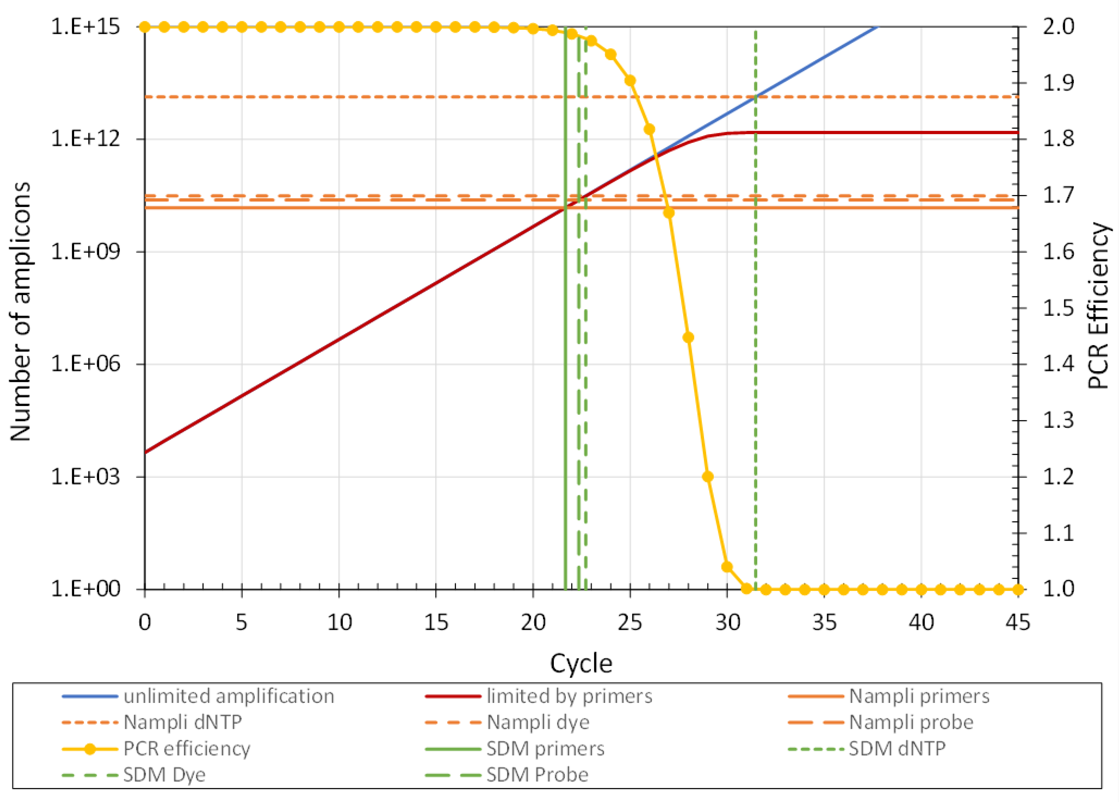
The above description of the different reaction components shows that for a specific standardized PCR design, the number of amplicons that can be generated (Nampli) in a reaction before the PCR efficiency drops 0.01 can be calculated from the chosen amplicon length, primer lengths and the concentrations of each of the three reaction components: the primers, the dNTP and either the dye or the probe concentration. These three calculations will result in three different Nampli values (Figure 4). The lowest of these Nampli values identifies the rate-limiting reaction component and its value determines the number of amplicons at which every reaction in the run will reach its SDM. Note that the actual SDM value depends on the unknown Ncopy in the reaction. With the observed SDM and the PCR efficiency (Eamc), off course both determined from the amplification curve of the respective reaction, the number of target molecules at the start of the PCR can now be calculated as Ncopy = Nampli / EamcSDM. As described above, the least variation in Ncopy will be reached when the Eamc in this equation is determined as the mean Eamc of all reactions with the same target [18].
3.4.6. Relative Expression and Normalisation Using Ncopy
As described above, in experimental research, the expression of a gene of interest is generally reported relative to the expression of a set of validated reference genes [2,32]. To this end the expression of the gene of interest is divided by the average expression of the reference genes, calculated as the geometric mean of the expression of the reference genes per sample. This procedure can also be applied to Ncopy values. However, this regretfully leads to loss of information about the absolute gene expression level because the result of this calculation is a fold difference compared to the reference genes. It is a pity that we thus loose the informative clarity of the absolute Ncopy values that we have just determined. However, with a simple extra step the absolute copy number can be retained. By definition, the average expression of the reference genes is the same for all samples in the experiment. Therefore, the above relative results will again reflect absolute copy number when they are multiplied by the geometric mean of the Ncopy values of all reference genes in all samples in the experiment.
4. Discussion and General Conclusions
Taken together, as discussed and illustrated above one can calculate the target quantity in the reaction at the start of the PCR (Ncopy) from the known amount of each of the reaction components in a given PCR, its PCR efficiency (Eamc) and SDM determined from the amplification curve. This Ncopy is assay, machine and laboratory independent and allows direct comparison of qPCR data between different laboratories and provides a very intuitive and easy to interpret absolute quantitative result. A goal that, despite the efforts to standardize the reporting of all steps of a qPCR experiment [2,5], was never reached. In our view, reporting Ncopy rather than Cq, solves most of the reproducibility issues of qPCR [8].
A few considerations have to be addressed before implementing the discussed limiting component approach to determine Ncopy. Firstly, one should take into account that SDM is defined as the fractional cycle at which the PCR efficiency has decreased with 0.01 from its initial value. However, in the calculation of Ncopy, the original efficiency value, which by now deviates 0.01 from the observed value, is used. The simulation of the role of primer concentrations shows that this discrepancy leads to a negative bias of 0.005 in Ncopy. Compared to other errors in qPCR, this bias can be considered to be negligible.
Secondly, the simulations of Dye and dNTP limits revealed that both components show an abrupt decrease of the observed PCR efficiency within one cycle. Because, contrary to the situation of the primer hybridisation, we are not aware of a model to describe the efficiency loss within this cycle, it was not possible to calculate an exact SDM from the simulated amplification curve. However, the fact that the expected SDM always falls within this cycle shows that the determined limits, and thus Nampli, for those reaction components are most probably correct.
Finally, we are aware that a wide implementation of this limiting component approach requires that the qPCR users know the exact composition of their reaction mixes. This requirement will increase the awareness of the need for standardisation of qPCR [2] and hopefully convinces manufactures of qPCR kits to disclose the compositions of the master mixes. On the other hand, the required calculation of Nampli per reaction component will give insight into the rate limiting factors in the PCR assay and may help with optimisation of the qPCR.
Supplementary Materials
Limiting_concentrations_in_qPCR.xlsx.
Author Contributions
Both authors designed and wrote this review.
Funding
This research received no external funding.
Institutional Review Board Statement
Not applicable.
Informed Consent Statement
Not applicable.
Conflicts of Interest
The authors declare no conflicts of interest.
References
- Derveaux, S.; Vandesompele, J.; Hellemans, J. How to do successful gene expression analysis using real-time PCR. Methods 2010, 50, 227–230. [Google Scholar] [CrossRef] [PubMed]
- Bustin, S. A.; Ruijter, J. M.; van den Hoff, M. J. B.; Kubista, M.; Pfaffl, M. W.; Shipley, G. L.; Tran, N.; Rodiger, S.; Untergasser, A.; Mueller, R.; Nolan, T.; Milavec, M.; Burns, M. J.; Huggett, J. F.; Vandesompele, J.; Wittwer, C. T., MIQE 2.0: Revision of the Minimum Information for Publication of Quantitative Real-Time PCR Experiments Guidelines. Clinical chemistry 2025.
- Larkin, S. E.; Holmes, S.; Cree, I. A.; Walker, T.; Basketter, V.; Bickers, B.; Harris, S.; Garbis, S. D.; Townsend, P. A.; Aukim-Hastie, C. , Identification of markers of prostate cancer progression using candidate gene expression. Br.J.Cancer 2012, 106, 157–165. [Google Scholar] [CrossRef] [PubMed]
- Bustin, S. A. , Why the need for qPCR publication guidelines?-The case for MIQE, Methods. Methods 2010. [Google Scholar] [CrossRef] [PubMed]
- Bustin, S. A.; Benes, V.; Garson, J. A.; Hellemans, J.; Huggett, J.; Kubista, M.; Mueller, R.; Nolan, T.; Pfaffl, M. W.; Shipley, G. L.; Vandesompele, J.; Wittwer, C. T. , The MIQE guidelines: minimum information for publication of quantitative real-time PCR experiments. Clin.Chem. 2009, 55, 611–622. [Google Scholar] [CrossRef]
- Tichopad, A.; Kitchen, R.; Riedmaier, I.; Becker, C.; Stahlberg, A.; Kubista, M. , Design and optimization of reverse-transcription quantitative PCR experiments. Clin.Chem. 2009, 55, 1816–1823. [Google Scholar] [CrossRef]
- Bivins, A.; Kaya, D.; Bibby, K.; Simpson, S. L.; Bustin, S. A.; Shanks, O. C.; Ahmed, W. , Variability in RT-qPCR assay parameters indicates unreliable SARS-CoV-2 RNA quantification for wastewater surveillance. Water Res 2021, 203, 117516. [Google Scholar] [CrossRef]
- Ruiz-Villalba, A.; Ruijter, J. M.; van den Hoff, M. J. B. , Use and Misuse of Cq in qPCR Data Analysis and Reporting. Life (Basel) 2021, 11, 496. [Google Scholar] [CrossRef]
- Bustin, S.; Nolan, T. , Talking the talk, but not walking the walk: RT-qPCR as a paradigm for the lack of reproducibility in molecular research. Eur J Clin Invest 2017, 47, 756–774. [Google Scholar] [CrossRef]
- Ramakers, C.; Ruijter, J. M.; Lekanne Deprez, R. H.; Moorman, A. F. M. , Assumption-free analysis of quantitative real-time polymerase chain reaction (PCR) data. Neurosci.Lett. 2003, 339, 62–66. [Google Scholar] [CrossRef]
- Ruijter, J. M.; Ramakers, C.; Hoogaars, W. M.; Karlen, Y.; Bakker, O.; van den Hoff, M. J.; Moorman, A. F. , Amplification efficiency: linking baseline and bias in the analysis of quantitative PCR data. Nucleic Acids Res. 2009, 37, e45. [Google Scholar] [CrossRef]
- Ruijter, J. M.; Barnewall, R. J.; Marsh, I. B.; Szentirmay, A. N.; Quinn, J. C.; van Houdt, R.; Gunst, Q. D.; van den Hoff, M. J. B. , Efficiency-correction is required for accurate qPCR analysis and reporting. Clinical chemistry 2021, 67, 829–842. [Google Scholar] [CrossRef] [PubMed]
- Karsai, A.; Muller, S.; Platz, S.; Hauser, M. T. , Evaluation of a homemade SYBR green I reaction mixture for real-time PCR quantification of gene expression. Biotechniques 2002, 32, 790–2, 794–6. [Google Scholar] [CrossRef] [PubMed]
- Vandesompele, J.; De Paepe, A.; Speleman, F. , Elimination of primer-dimer artifacts and genomic coamplification using a two-step SYBR green I real-time RT-PCR. Anal Biochem 2002, 303, 95–8. [Google Scholar] [CrossRef]
- Ruijter, J. M.; Lorenz, P.; Tuomi, J. M.; Hecker, M.; van den Hoff, M. J. , Fluorescent-increase kinetics of different fluorescent reporters used for qPCR depend on monitoring chemistry, targeted sequence, type of DNA input and PCR efficiency. Mikrochim.Acta 2014, 181, 1689–1696. [Google Scholar] [CrossRef]
- Rasmussen, R., Quantification on the LightCycler instrument. In Rapid Cycle Real-Time PCR: methods and applications, Meuer, S.; Wittwer, C.; Nakagawara, K., Eds. Springer: Heidelberg, 2001; pp 21-34.
- Rebrikov, D. V.; Trofimov, D. I. , Real-time PCR: a review of approaches to data analysis. Appl Biochem Microbiol 2006, 42, 455–463. [Google Scholar] [CrossRef]
- Ruijter, J. M.; Pfaffl, M. W.; Zhao, S.; Spiess, A. N.; Boggy, G.; Blom, J.; Rutledge, R. G.; Sisti, D.; Lievens, A.; De Preter, K.; Derveaux, S.; Hellemans, J.; Vandesompele, J. , Evaluation of qPCR curve analysis methods for reliable biomarker discovery: Bias, resolution, precision, and implications. Methods 2013, 59, 32–46. [Google Scholar] [CrossRef]
- Livak, K. J.; Schmittgen, T. D. , Analysis of relative gene expression data using real-time quantitative PCR and the 2(-Delta Delta C(T)) method. Methods 2001, 25, 402–408. [Google Scholar] [CrossRef]
- Nolan, T.; Hands, R. E.; Bustin, S. A. , Quantification of mRNA using real-time RT-PCR. Nat.Protoc. 2006, 1, 1559–1582. [Google Scholar] [CrossRef]
- Ruijter, J. M.; Ruiz-Villalba, A.; van den Hoff, M. J. B. , Cq Values Do Not Reflect Nucleic Acid Quantity in Biological Samples. Clinical chemistry 2021, 68, 7–9. [Google Scholar] [CrossRef]
- Pfaffl, M. W. , A new mathematical model for relative quantification in real-time RT-PCR. Nucleic Acids Res 2001, 29, e45. [Google Scholar] [CrossRef]
- Walker, N. J., Tech. Sight. A technique whose time has come. Science 2002, 296, 557–559. [Google Scholar] [CrossRef] [PubMed]
- Ginzinger, D. G. , Gene quantification using real-time quantitative PCR: an emerging technology hits the mainstream. Exp.Hematol. 2002, 30, 503–512. [Google Scholar] [CrossRef] [PubMed]
- Lekanne Deprez, R. H.; Fijnvandraat, A. C.; Ruijter, J. M.; Moorman, A. F. M. , Sensitivity and accuracy of quantitative real-time polymerase chain reaction using SYBR green I depends on cDNA synthesis conditions. Anal Biochem. 2002, 307, 63–69. [Google Scholar] [CrossRef] [PubMed]
- Zhao, S.; Fernald, R. D. , Comprehensive algorithm for quantitative real-time polymerase chain reaction. J.Comput.Biol. 2005, 12, 1047–1064. [Google Scholar] [CrossRef]
- Rutledge, R. G.; Stewart, D. , Assessing the performance capabilities of LRE-based assays for absolute quantitative real-time PCR. PLoS.ONE. 2010, 5, e9731. [Google Scholar] [CrossRef]
- Guescini, M.; Sisti, D.; Rocchi, M. B.; Stocchi, L.; Stocchi, V. , A new real-time PCR method to overcome significant quantitative inaccuracy due to slight amplification inhibition. BMC.Bioinformatics. 2008, 9, 326. [Google Scholar] [CrossRef]
- Spiess, A. N.; Deutschmann, C.; Burdukiewicz, M.; Himmelreich, R.; Klat, K.; Schierack, P.; Rodiger, S. , Impact of smoothing on parameter estimation in quantitative DNA amplification experiments. Clinical chemistry 2015, 61, 379–88. [Google Scholar] [CrossRef]
- Untergasser, A.; Ruijter, J. M.; Benes, V.; van den Hoff, M. J. B. , Web-based LinRegPCR: application for the visualization and analysis of (RT)-qPCR amplification and melting data. BMC bioinformatics 2021, 22, 398. [Google Scholar] [CrossRef]
- Ruiz-Villalba, A.; Ziogas, A.; Ehrbar, M.; Perez-Pomares, J. M. , Characterization of epicardial-derived cardiac interstitial cells: differentiation and mobilization of heart fibroblast progenitors. PLoS One 2013, 8, e53694. [Google Scholar] [CrossRef]
- Vandesompele, J.; De Preter, K.; Pattyn, F.; Poppe, B.; Van Roy, N.; De Paepe, A.; Speleman, F. , Accurate normalization of real-time quantitative RT-PCR data by geometric averaging of multiple internal control genes. Genome Biol. 2002, 3, RESEARCH0034. [Google Scholar] [CrossRef]
- Hellemans, J.; Mortier, G.; De, P. A.; Speleman, F.; Vandesompele, J. , qBase relative quantification framework and software for management and automated analysis of real-time quantitative PCR data. Genome Biol. 2007, 8, R19. [Google Scholar] [CrossRef] [PubMed]
- Bustin, S. A. , Quantification of mRNA using real-time reverse transcription PCR (RT-PCR): trends and problems. J.Mol.Endocrinol. 2002, 29, 23–39. [Google Scholar] [CrossRef] [PubMed]
- Vermeulen, J.; de Preter, K.; Naranjo, A.; Vercruysse, L.; Van Roy, N.; Hellemans, J.; Swerts, K.; Bravo, S.; Scaruffi, P.; Tonini, G. P.; De Bernardi, B.; Noguera, R.; Piqueras, M.; Canete, A.; Castel, V.; Janoueix-Lerosey, I.; Delattre, O.; Schleiermacher, G.; Michon, J.; Combaret, V.; Fischer, M.; Oberthuer, A.; Ambros, P. F.; Beiske, K.; Benard, J.; Marques, B.; Rubie, H.; Kohler, J.; Potschger, U.; Ladenstein, R.; Hogarty, M. D.; McGrady, P.; London, W. B.; Laureys, G.; Speleman, F.; Vandesompele, J. , Predicting outcomes for children with neuroblastoma using a multigene-expression signature: a retrospective SIOPEN/COG/GPOH study. Lancet Oncol. 2009, 10, 663–671. [Google Scholar] [CrossRef] [PubMed]
- Ruiz-Villalba, A.; van Pelt-Verkuil, E.; Gunst, Q. D.; Ruijter, J. M.; van den Hoff, M. J. , Amplification of nonspecific products in quantitative polymerase chain reactions (qPCR). Biomol Detect Quantif 2017, 14, 7–18. [Google Scholar] [CrossRef]
- Brankatschk, R.; Bodenhausen, N.; Zeyer, J.; Burgmann, H. , Simple absolute quantification method correcting for quantitative PCR efficiency variations for microbial community samples. Appl Environ Microbiol 2012, 78, 4481–9. [Google Scholar] [CrossRef]
- Shipley, G., Assay Design for Real-Time qPCR. In PCR Technology: Current Innovations, Third Edition, Nolan, T.; Bustin, S. A., Eds. CRC Press: London, New York, 2013; pp. 177–199.
- de Ronde, M. W.; Ruijter, J. M.; Lanfear, D.; Bayes-Genis, A.; Kok, M.; Creemers, E.; Pinto, Y. M.; Pinto-Sietsma, S. J., Practical data handling pipeline improves performance of qPCR-based circulating miRNA measurements. RNA 2017.
- Fang, Y.; Liao, P.; Chen, Z.; Chen, H.; Wu, Y.; Li, S.; Deng, Y.; He, N. , Improvement and Application of qPCR (Real-Time Quantitative Polymerase Chain Reaction) Data Processing Method for Home-Made Integrated Nucleic Acid Detection System. J Nanosci Nanotechnol 2020, 20, 7369–7375. [Google Scholar] [CrossRef]
- Tichopad, A.; Dilger, M.; Schwarz, G.; Pfaffl, M. W. , Standardized determination of real-time PCR efficiency from a single reaction set-up. Nucleic Acids Res 2003, 31, e122. [Google Scholar] [CrossRef]
- Spiess, A. N.; Feig, C.; Ritz, C. , Highly accurate sigmoidal fitting of real-time PCR data by introducing a parameter for asymmetry. BMC.Bioinformatics. 2008, 9, 221. [Google Scholar] [CrossRef]
- Gevertz, J. L.; Dunn, S. M.; Roth, C. M. , Mathematical model of real-time PCR kinetics. Biotechnol.Bioeng. 2005, 92, 346–355. [Google Scholar] [CrossRef]
- Zipper, H.; Brunner, H.; Bernhagen, J.; Vitzthum, F. , Investigations on DNA intercalation and surface binding by SYBR Green I, its structure determination and methodological implications. Nucleic Acids Res 2004, 32, e103. [Google Scholar] [CrossRef]
- Wittwer, C. T.; Herrmann, M. G.; Moss, A. A.; Rasmussen, R. P. , Continuous fluorescence monitoring of rapid cycle DNA amplification. BioTechniques 1997, 22, 130–138. [Google Scholar] [CrossRef]
- Mao, F.; Leung, W. Y.; Xin, X. , Characterization of EvaGreen and the implication of its physicochemical properties for qPCR applications. BMC Biotechnol 2007, 7, 76. [Google Scholar] [CrossRef]
Figure 1.
Amplification curves and quantification threshold setting. (a) Amplification curves of a set of positive control reactions [12] plotted on a linear fluorescence scale; (b) The same amplification curves plotted on a logarithmic scale. The straight exponential phase is found between the blue lines. The green line in panels a and b is an example of a set fluorescence threshold (Fq); (c) Range of Cq values (mean and standard deviation) obtained after setting the quantification threshold (Fq) from low to high.
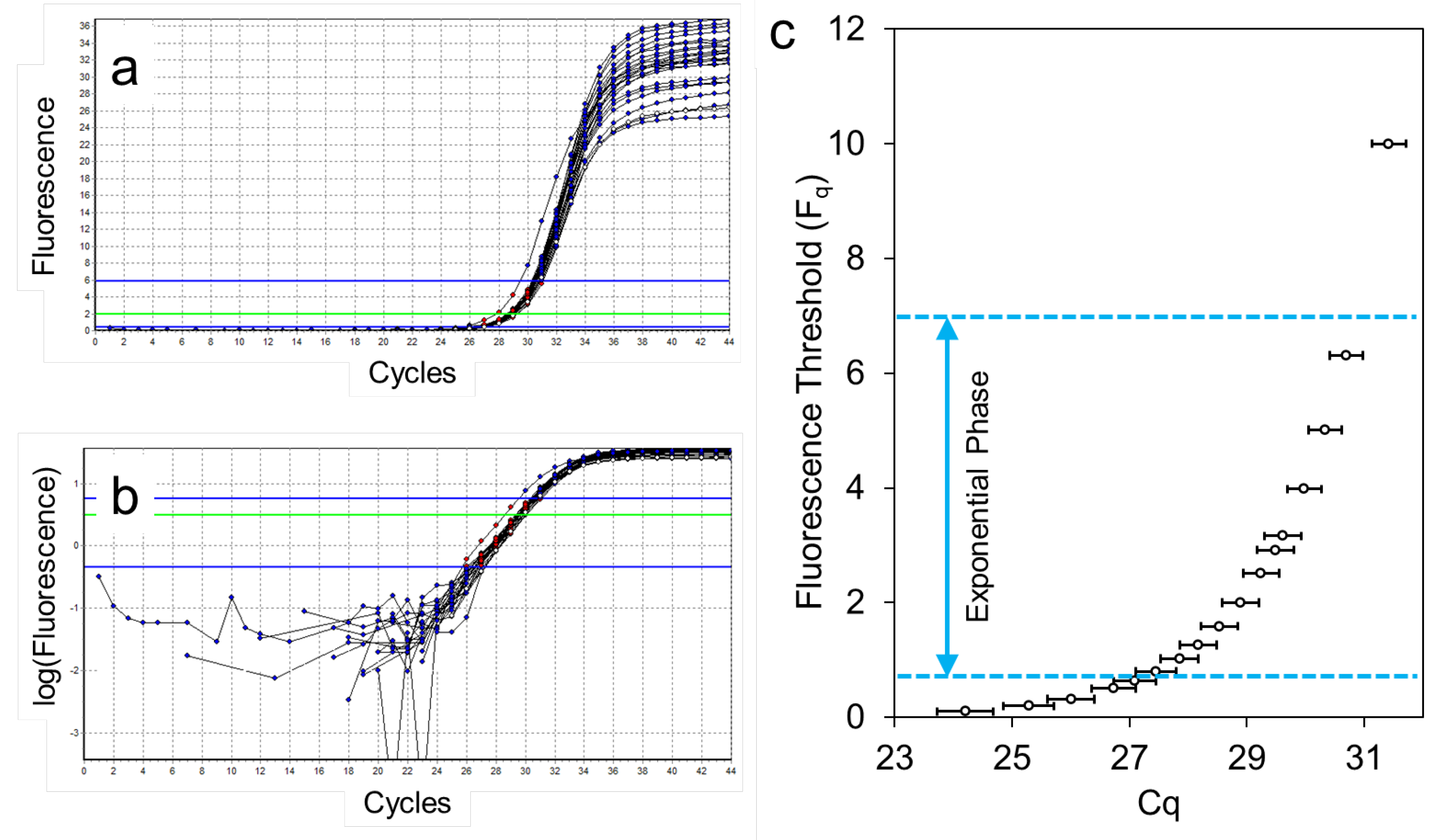
Figure 2.
Comparison of baseline correction by LinRegPCR [11] and the qPCR system. (a) Raw fluorescence data exported by the qPCR system. Colours indicate the number of target copies in the reaction; (b) Amplification curves after baseline correction with LinRegPCR; (c) Amplification curves after system baseline correction with a trendline fitted to the data points in cycle 2-5; (d) Relation between the fluorescence of the target quantity (F0) and the input copy number determined after baseline correction by LinRegPCR (blue) or the qPCR System (orange).
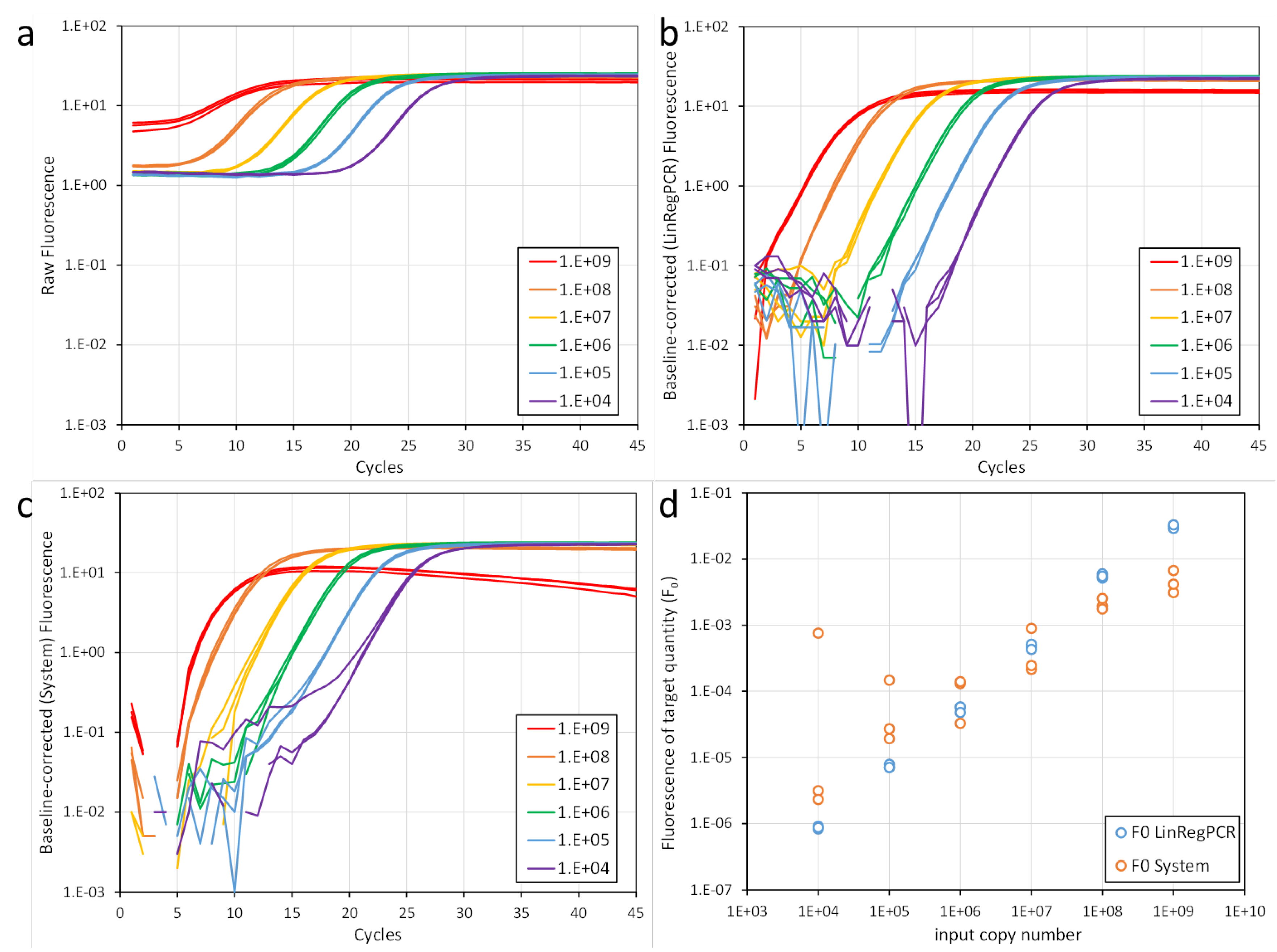
Figure 3.
Limiting reaction components in PCR. The panels show amplification curves, SDM and observed efficiency for different simulated scenarios. Except for the variations per panel the other reaction components are present in standard concentration of the reaction mix (Ncopy: 4500, reaction volume: 10 uL, Primers: 250 nM, Dye: 98 nM, dNTP: 0.2 mM, Probes: 400 nM, Amplicon length 200bp, Primer lengths 20bp.); (a) Amplification curves for different number of targets at the start of the reaction (Ncopy, 4500, 1000 and 200) in combination with different primer concentrations (50, 250 and 1000 nM); (b) and (c). Summary of the outcome of a PCR simulation when different amplicon length (200 and 800bp) in relation to the limit on PCR due to Dye (b) and to dNTP (c) are evaluated; (d) Summary of the outcome of a PCR simulation evaluating the same concentration of hydrolysis and hybridisation probes. Note that although the amplification curves for the hydrolysis and hybridisation probes differ but the other parameters behave the same.
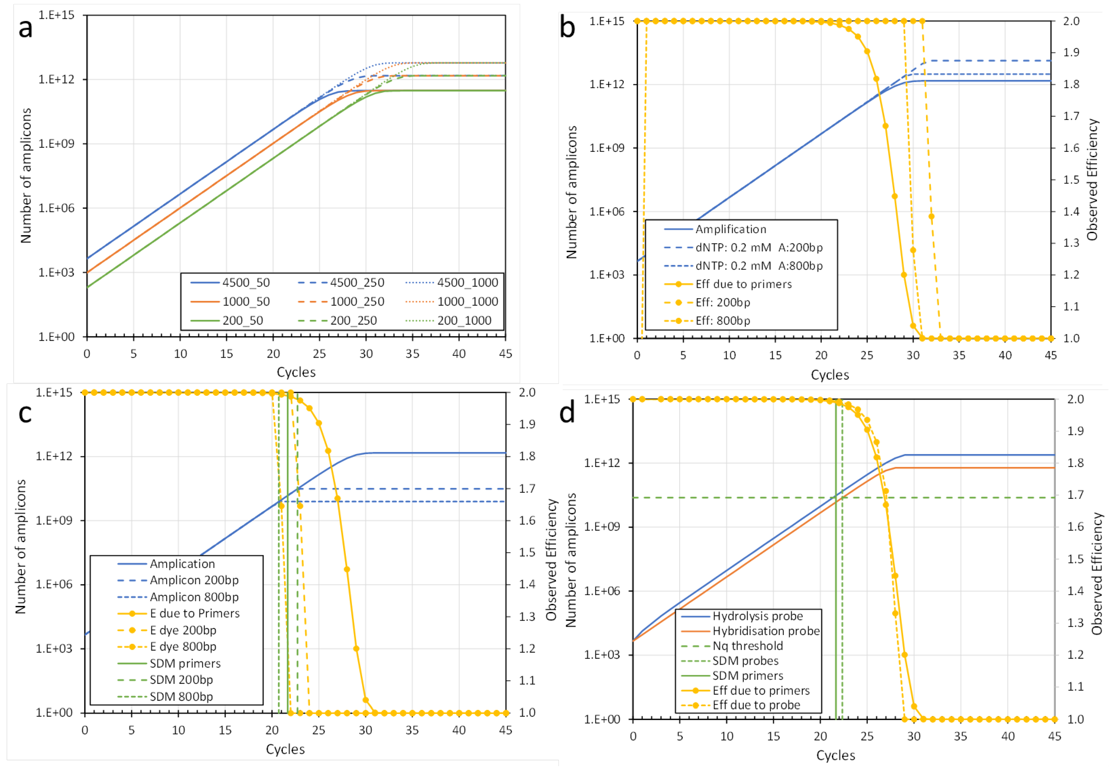
Figure 4.
Determining the limiting reaction component in PCR. The figure shows the amplification curve limited by the primer concentration and the SDM’s and Nampli values resulting from the other reaction components and variables for the standard reaction composition: Ncopy: 4500, reaction volume: 10 uL, Primers: 250 nM, Dye: 98 nM, dNTP: 0.2 mM, Probes: 400 nM, Amplicon length 200bp, Primer lengths 20bp.
Disclaimer/Publisher’s Note: The statements, opinions and data contained in all publications are solely those of the individual author(s) and contributor(s) and not of MDPI and/or the editor(s). MDPI and/or the editor(s) disclaim responsibility for any injury to people or property resulting from any ideas, methods, instructions or products referred to in the content. |
© 2025 by the authors. Licensee MDPI, Basel, Switzerland. This article is an open access article distributed under the terms and conditions of the Creative Commons Attribution (CC BY) license (http://creativecommons.org/licenses/by/4.0/).
Copyright: This open access article is published under a Creative Commons CC BY 4.0 license, which permit the free download, distribution, and reuse, provided that the author and preprint are cited in any reuse.


