
Submitted:
29 October 2025
Posted:
31 October 2025
You are already at the latest version
Abstract
The Newcomb-Benford Law (NBL) suggests that the smaller digits of significands represented in place-value notation are more likely to appear in real-life numerical datasets. We propose that similar laws exist regarding the prime factorization of these significands.
By the fundamental theorem of arithmetic, we can express a natural number as an ordinal-ascending sequence of ordinal-multiplicity pairs representing the prime factors by which N is divisible. We refer to this as the Standard Ordinal-Exponent representation (SOE). The costs of the positional and SOE representations interconnect through the double logarithmic scale; the size of a number written in positional notation has the same order of growth as the exponential of the SOE sequence length. Based on the SOE representation, we submit a battery of laws exhibiting the prevalence of the minor prime powers across the natural numbers, to wit, the probability of a prime relative to the factorization set, the probability and possibility of the smallest prime ordinal, the probability of the number of participants in an interaction (regarding and disregarding multiplicity), the probability and possibility of a prime divisor with multiplicity, the probability of a prime exponent, and the probability of the largest prime exponent.
Then, we factorize two NBL-compliant datasets to investigate key properties of primality: a 300-entry dataset comprising mathematical and physical constants (CT), and another containing 1,080 entries of world population data (WP). For both, we examine the energy function E(N)=p_N/N, the omega functions ω(N) (number of distinct prime factors) and Ω(N) (total number of prime factors), the divisor functions d(N) (number of divisors) and σ(N) (sum of divisors), as well as the share of rough-smooth numbers, the growth of highly composite numbers, and the prime-counting π(N) and totient φ(N) functions. Besides, we confirm compliance with the laws above and analyze the internal count of primes, the density of the largest prime ordinal, the internal growth of totatives and non-totatives, the density of k-almost primes, and the distribution of the pairwise greatest common divisor.
CT and WP are chunks of nature. Indeed, we can identify natural datasets by testing their conformance to NBL or to any of the criteria we postulate. We also emphasize that the artanh function prominently appears throughout our analysis, suggesting that the concept of conformality governs our perception of the external world, bridging information between the harmonic scale (global) and our logarithmic scale (local).
Keywords:
newcomb-benford law
; probability mass function
; prime factorization
; standard ordinal-exponent representation
; representational cost
; double harmonic scale
; primality scale
; double logarithmic scale
; divisibility
; k-almost prime
; relative prime
; natural dataset
; lognormal distribution
; artanh function
MSC: 11A25—Arithmetic functions; related numbers; 11A41—Primes; 11A51—Factorization; primality; 11K65—Arithmetic functions in probabilistic number theory; 11L20—Sums over primes; 11N05—Distribution of primes; 11N64—Other results on the distribution of values or the characterization of arithmetic functions; 60-08—Computational methods for problems pertaining to probability theory; 60-11—Research data for problems pertaining to probability theory
1. Introduction
How does the universe build large structures from small components? This article on elementary algebra examines the set of natural numbers greater than 2, , through their factorization into the set of prime numbers, namely the subset of that cannot be expressed as a product of two or more smaller numbers. In the analytic theory of prime arithmetic functions, we propose several probability mass and possibility distribution functions that are biased towards minor prime factors, alongside the well-known NBL (Newcomb-Benford Law). The NBL describes the frequency distribution of the leading digit in many naturally occurring numerical datasets written in standard positional notation [1]; approximately of these numbers start with the digit one, while below begin with the digit nine [2]. Do primes have similar laws?
It is pertinent to highlight how the theory connects prime numbers to NBL. In general, the sequence of prime numbers is not Benford [3]. Moreover, from the prime number theorem (see Section 3.3), we can infer that the distribution of the first digit of prime numbers approaches uniformity as the scale factor increases [4]. At this point, the research on the topic becomes twofold. On the one hand, although there is no uniform probability on any infinite countable set, i.e., there is no natural density, any well-defined density that satisfies certain intuitive conditions for prime numbers, e.g., lack of bias towards specific subsets of primes, will lead to NBL [5]. Especially, prime numbers comply with NBL in both logarithmic and zeta densities [6]; e.g., the set of primes with a leading digit of 1 has logarithmic density (see subsection of [7]). On the other hand, we can generalize the NBL to cope with the primes by constraining the intervals of primes under consideration. The leading digits in the sequence of prime numbers follow a generalized NBL that accounts for the varying density of primes found within intervals of the form [8]. This approach reveals a scale-dependent -power law that simplifies to a uniform distribution as the number of primes examined approaches infinity, i.e., as vanishes. By focusing the analysis on intervals between two adjacent integral powers of ten and applying the density , where denotes the set of primes in containing the subset with a leading digit d, we also arrive at NBL as s approaches infinity.
Notwithstanding, Kossovsky [9] cautions that ” prime numbers do not care much about integral-powers-of-ten intervals [...] Surely they also do not pay any attention whatsoever to the particular number systems invented by the various civilizations scattered about randomly across the universe, as they float eternally up there well above all such lowly and arbitrary local inventions. Conclusions about the primes in digital Benford’s Law [...] do not interest the primes much.” We agree. While digit pattern analysis can reveal valuable insights that may not be evident in analytical studies or visual inspections, from a physics perspective, it is more functional to uncover new rules by examining the prime factor ordinals and exponents of an organic dataset. Despite confining the information to a particular domain, the acquired knowledge is more fundamental because it is independent of the number system and represents nature’s realities.
Suppose NBL reflects the occurrence probability of the digits in a sample of data represented in place-value notation. In that case, it is logical to expect a monotonically decreasing distribution regulating their prime factorization. To analyze the number theory associated with a dataset, we have introduced the SOE (Standard Ordinal-Exponent) representation of a number , an ordinal-ascending sequence of the prime factors by which N is divisible, where a prime ordinal and exponent (or multiplicity) represent the factor . The nexus between positional notation and primality lies in the number of distinct prime factors rather than in the individual digits. When written in positional notation, N’s size grows exponentially with respect to the average growth of , namely , and N’s representational cost is about , an information-theoretic measure of N’s energy, defined as .
Taking the SOE representation as a basis, we examined two representative natural datasets. The first dataset includes 300 entries of mathematical and physical constants (CT), while the second dataset contains 1,080 entries of world population data (WP). Both CT and WP datasets conform to the NBL. Datasets that comply with the NBL provide valuable insights when analyzed in relation to the chief functions of number theory. These include the energy function , the omega functions (number of distinct prime factors) and (total number of prime factors), the divisor functions (number of divisors) and (sum of divisors), as well as the distribution of rough and smooth numbers, the growth of highly composite numbers, the prime-counting function, and the totient function. We also study the internal growth of and after sorting the dataset, i.e., or . The joint analysis of these number-theoretic functions across natural datasets is a novel area of scientific research.
We acknowledge the existence of numerous theoretical findings in this field. The fundamental Erdos-Kac theorem in probabilistic number theory [10] states that a standard normal distribution fits the probability distribution of . This theorem supports the aforesaid link between positional and SOE notations, and hence between NBL and primality. Significantly, many of the theoretical concepts discussed in this work can be traced back to the works [11,12]. Additionally, relevant material included by [13] in sections 2.6 and 2.7 also supports our discussion.
We have employed the Anderson-Darling, Kolmogorov-Smirnov, Kuiper, Pearson’s chi-squared, Watson U², and Cramér-von Mises goodness-of-fit tests for statistical analysis. However, these methods often reject the null hypothesis even when there is explicit visual agreement, due to the sample size. To mitigate excess power in samples with more than 100 elements, we use the Relative Root Mean Squared Error (RRMSE), which provides a normalized measure of the mean absolute deviation between the empirical and expected distributions, as described by [14]. We base the thresholds for interpreting the outcomes on the guidelines from [15].
The literature often suggests that physics emerges from mathematics, without proof. However, the set of laws governing ” the minor” we posit does sustain this hypothesis, which may reveal a fundamental aspect of the universe’s structure and dynamics. Much of the theory not addressed in this paper deserves similar attention. We do not cover areas such as the Möbius function, Liouville lambda, and radical functions intentionally to keep our study focused. Additionally, applying all current theories to a substantial collection of natural datasets would require many years. Other gaps identified by the reader are probably due to feasibility constraints rather than a lack of interest.
Specifically, our study presents a series of laws that confirm the significance of minor prime powers in subsets of , including the probability of a prime disregarding multiplicity within the factorization set, the probability and possibility of the SPO (Smallest Prime Ordinal), the probability of the number of participants in an interaction (in two versions), the distribution of a prime power divisor within the factorization set, the possibility of a prime power divisor relative to the dataset size, the general probability of a prime exponent, and the probability of the LPE (Largest Prime Exponent). We are not aware of any existing laws in the literature that encompass these findings. Additionally, we extend the applicability of our results and conclusions to real-life numerical datasets. In relation to ranges of naturals, CT, and WP, we also examine the informational energy of a prime, the growth of the number of primes, highly composite numbers, and totatives, as well as the density of the LPO (Largest Prime Ordinal), k-almost primes, and square-free k-almost primes, the growth of intratotatives and non-intratotatives, and the probability of the Greatest Common Divisor (GCD). From the information gathered, we derive a battery of rules to assess the naturalness of a dataset.
Another key result is that many distributions exhibit characteristics similar to those of a lognormal distribution. A random variable is lognormal if its logarithm follows a Gaussian distribution. Conversely, the exponential of a normal random variable results in a lognormal distribution. We often encounter the lognormal distribution when analyzing observational measurements in science and engineering. The usual distribution is, in fact, the lognormal distribution [16], which is the maximum entropy probability distribution for a random variable whose logarithm has fixed mean and variance [17]. Depending on these parameters, a lognormal variable’s distribution may either be monotonically decreasing or present a global peak (the mode). Moreover, we can adapt the lognormal model to fit the NBL distribution as the scale increases [18]. In essence, the lognormal distribution encompasses the NBL distribution to such an extent that we can use it to test for statistical compliance with the NBL [19].
Lognormal distributions are instances of ” artanh distributions.” A random variable follows an artanh distribution if its logarithm delivers an LFT (Linear Fractional Transformation) [20]. When we zoom in sufficiently on the curve’s symmetry center, the artanh outline appears as a straight line. Likewise, it resembles an exponential or logarithmic curve near the boundaries when rotated. For example, when appropriately centered, scaled, and bounded (as shown in Figure 10 in green), the outline of the WP energy aligns with the conformal 1-ball model (see section 4 of [21]); ” outside a coding source, the information resides on a harmonic scale, while inside, a logarithmic scale accommodates local Bayesian data.” Therefore, a plausible explanation for our observations is that the original data are generated globally from a harmonic scale. We then adapt the empirical data locally to our logarithmic scale through a conformal LFT transformation, allowing us to perceive a world of ” normality” in many instances.
This article has the following structure. We redefine the representational cost of a number and its informational energy, finding that a double logarithmic scale bridges the positional and SOE notations. We analyze the growth of divisibility and the distribution of prime numbers. Assuming the canonical PMF (Probability Mass Function), namely , we derive the law for the minor prime as well as the probabilistic and possibilistic laws for the SPO. Next, we review the density of almost-primes, the laws governing interactions, the growth of relative primes, and the law of the pairwise GCD. Further, we derive the laws governing the frequency of divisors (considering multiplicity), exponents, and the LPEs. Finally, we compare the theory embracing these topics with the prime factorizations of CT and WP, fragments of nature that generate number-theoretic patterns typical of . In particular, the relativistic conformal 1-ball model can explain the many observed artanh curve segments. The concluding remarks summarize the proposed laws and criteria we can use, in addition to NBL, to assess the naturalness of a dataset, and discuss the fundamental role they play as principles of a general theory of the minor prime factors.
2. Representational Cost, Information, and Energy
From an IT perspective, the cosmos must support a consistent numbering system while also being flexible and agile from an evolutionary standpoint. To achieve these goals, a crucial requirement is reasonable cost control.
We can define the cost C of representing a number in standard positional notation with radix () [22] as
The formula gauges how compacted a datum is.
We can approximately take the representational cost of as (twice) the Hartley information of sequences formed by n successive selections from a set of N elements. The elements or symbols of the set represent a fixed range of possible alternatives prior to each selection that cause ambiguity to the observer (receiver of the message, experimenter, or the like) [23]. The total number of possible sequences of selections from the set is [24]. The formula
gives the amount of information conveyed by one among all these sequences, which is the only function satisfying the axioms of monotonicity () and additivity () for any proportionality constant and radix r. Choosing , , and , we add the axiom of normalization , so that the cost (i.e., inherent information) of the r-ary () representation of is
Indeed, the Hartley information is a normalized cost measured in bits (), trits (), or dits (), depending on the coding radix. Note that this Hartley information interpretation of the cost is dual to the standard interpretation given to (1). The latter is spatial, while the former is temporal, because it is the duration of the process of choosing among N possibilities repeated at most r times. Ultimately, we must either minimize the space occupied or the time required to process the number, or both.
Nonetheless, the cost estimated by Equations (1) and (2) might be insufficient for calculation purposes. In arithmetic, the addition of a number to another that is several orders of magnitude smaller hardly alters the value of the former. What is the use of adding googol to 1, irrespective of the base? The biggest operands dominate the outcome of an unbalanced sum. In cosmology, for instance, distances and specific parameters require different techniques of approximate computation and estimation, allowing for adaptive precision [25].
More particularly, numerical computation by machines often leads to subtle rounding errors that can become gross errors in specific scenarios. In IEEE 754 standard notation, this problem arises when the CPU represents the two terms in a sum using the same power of two in order to apply the distributive property of multiplication. If , where p is the number of bits used for the mantissa, everything is all right [26]; otherwise, the consequences are unknown. Note that rounding errors are not specific to a system or notation; whenever we sum numbers that belong to too many different scales, or subtract one number from another that is very close, errors proliferate. To get around this situation, we should easily either access the order of magnitude of a number N (e.g., explicitly prepending to its representation) or calculate it as the exponential of its double logarithm, assuming that we can infer such data from its representation.
The point is that the double logarithmic and primality scales are linked. While the harmonic world connects with and logarithmic world through the asymptotic limit
where is the Nth harmonic number and the Euler-Mascheroni constant, the harmonic series of primes (i.e., the depleted harmonic series comprised by the reciprocals of all prime numbers) and the double logarithmic scale are interrelated by the asymptotic limit [12]
where
is the Nth element of the harmonic series of primes and is the Meissel-Mertens constant ([13], section ). In other words, expression (4) is the analog of (3) for primes, where and M play the role of and , respectively.
Interestingly, , so that . Thus, we position the primality scale between the double logarithmic and double harmonic scales; M represents the separation between the double logarithmic and primality scales, and represents the separation between the primality and double harmonic scales.
The curves of these three scales grow very slowly. If we want, say, to halve the area between e and , then x must ebb down to . In general, for a variable to scale by , the variable must transform in a double geometric manner, i.e., according to a tetration scheme . These ” second-order hyperbolic” scales enable efficient calculations and thrifty management of large numbers. What happens at the gigantic, coarse upper levels necessarily ignores the fine-grained detail of the lower levels. In particular, the double logarithm appears frequently in quite diverse disciplines of mathematics and physics (e.g., in studies of complexity concerning fundamental lattice problems [27]).
The double logarithmic, primality, and double harmonic scales are intricately associated with factorization and divisibility. By the Erdos-Kac theorem of probabilistic number theory, they have, except for the separation constant, the same asymptotic order of growth as the average number of distinct prime factors of N, i.e.,
For example, , , , and .
In practice, defines a coding scheme that uses the logarithm or harmonic number of the order of magnitude of N rather than N itself. Thus, if nature calculates the size of an operand N via , 1 should directly or indirectly involve . Using a result from [28], we can define this total cost, or ” energy” , in terms of a tight explicit pair of bounds.
Definition 1.
The law of the minor inherent information states that the energy
of is within the bracket
Mind that the relative weight of the double logarithm with respect to the energy fades away as N goes to infinity. That is, as N grows, its energy jumps less, and gaps tend to disappear. If we divide the bracket by , then
What is the probabilistic meaning of ? It is the expected maximum load of balls across a collection of bins after throwing N balls into them one by one at random, where the sequence of target bins of throws is independent and identically distributed [29]. For example, we expect a maximum of balls across a million bins after randomly throwing a million balls into them.
A radix with a low average cost is economic (e.g., binary, ternary, or quaternary). We comply with the minimum information principle [30] when the derivative of (6) with respect to r vanishes, obtaining Euler’s number e. This constant represents the optimal radix choice [22].
In Section 8, we analyze how the informational energy, and hence the representational cost, grows in real-world datasets.
3. Overview of primality
3.1. The Ordinal-Exponent Representation
The factorization of a number determines its count of distinct prime factors.
Based on the unique prime factorization theorem [31], we can think of the set of all prime numbers, , as the atoms of so that we can express every natural greater than one as a unique finite product of primes (e.g., ). The ” arithmetic” of this prime factorization consists of binary operations (principally product, GCD, and least common multiple) yielding an output represented in terms of the prime factors of the operands. Whereas the canonical prime factorization stresses the use of primes themselves, we propose a representation that makes the prime ordinal explicit.
Definition 2.
TheSOE representationof is an ordinal-ascending sequence of prime factors (prime with ordinal and exponent or multiplicity ) by which N is divisible, so that
For example, (), (), (), and ().
Extending this representation to is trivial by inclusion of negative multiplicities (e.g., , with ), where positive and negative exponents are associated with the numerator and the denominator, respectively.
The primary purpose of the SOE representation is to extract the properties of the natural numbers by studying their prime factor ordinals and exponents. For instance, the prime signature of a natural [32] straightforwardly follows from this representation (e.g., 5635 has signature ), which in turn enables the calculation of many other important functions in number theory. Likewise, the length of a natural number in SOE representation is precisely the number of distinct prime factors , and the total number of prime factors is
For example, . As N climbs to infinity, the distribution of tends to a Gaussian with mean (4) and variance , and the distribution of to a Gaussian with mean and the same variance [33].
We define the number of divisors as
For example, , to wit , with distinct prime factors, namely , and , to wit , with distinct prime factors, namely .
The sum of positive divisors function for is
For instance, , namely {1, 5, 7, 23, 35, 49, 115, 161, 245, 805, 1127, 5635}, so that .
Algebraically, the SOE representation is very effective. If , then N is even; otherwise, it is odd. If , then N is odd and divisible by 3. If , then N is a prime number; if , then N is a composite number; if , then N is a prime power; and if , then N is a k-almost prime number. We can spot a square as having even exponents for all i, a cube as a number whose exponents are all divisible by 3, an n-free integer has no exponents (e.g., a square-free natural has no exponent ), and a powerful (or squareful) number has for all i. A natural number divides (written as ) if and only if .
Suppose a sample of natural numbers complies with NBL. In that case, we can presume that (SPO), (SPE, the Smallest Prime Exponent), (LPO), and (LPE), as well as the omega and divisors functions, will tend to the lowest values to maximize operability. In contrast, high values can reveal unworkability or instability. Moreover, SPO, SPE, LPO, and LPE are leading indicators of proclivity to interaction (e.g., prime powers are increasingly less robust and more vulnerable). Nevertheless, these values are insufficient to characterize a natural number. For instance, and both have , , , , , and ; they even have the same signature, , and . The difference between them is that . Interestingly, for increasing ranges of natural numbers, the log-plot of the sums of ordinals always approximates a segment of an artanh curve (see Figure 1).
Specifically, the LPO gives place to the concept of ” roughness” . A natural number N such that is -rough. Primes are -rough numbers, as is the product of two primes. Despite the name, the -rough numbers (https://oeis.org/A064052) are stable enough because ; we can consider roughness as a soft version of primality [34]. Natural numbers that are not -rough are -smooth (, https://oeis.org/A048098), which possess high values of . In the infinite limit, the rate of -rough against -smooth numbers is allegedly a constant, to wit (Schroeppel in [35], and [36]). Note that it is about a split. The expected value for of -roughness versus -smoothness is . We will analyze in Section 8 the extent to which CT and WP achieve such a split and -equilibrium
Likewise, the notions of ” smoothness” and ” roundness” overlap. A round number is the product of a substantial number of relatively small factors as compared to its neighboring numbers. Typical examples are 24 and 48 in decimal. The probability of roundness grows with the nearly interrelated omega functions; always , ([11], section ), and both functions have the same asymptotic order of growth. generally sticks very well (” usually not much larger ... nor smaller” ) to , much better than . Because the double logarithm grows so slowly, round numbers are tremendously rare (see section of [11]). The central property of round numbers is volatility (e.g., as reflected in a high ). As Hardy admits, one would expect large numbers mainly to be achieved by renouncing stability (i.e., producing a high ). However, as we will see in Section 7.2, we observe a tendency to produce large numbers by employing significant prime factors rather than multiple copies of small ones.
3.2. Growth of Divisibility
The relatively simple concept of divisibility is likely ubiquitous in the cosmos, up to a limit [37]. This section anticipates the content of the laws we will define in the following sections concerning the number of divisors.
Considering that the average order of the divisor function satisfies (see [11], section )
we can describe the round numbers as having many more divisors than their local mean. Moreover, the sum of divisors of round numbers is much higher than their neighborhood mean.
The average sum of divisors function of all naturals to is connected through to the natural logarithm ([11] theorem 320) by
where the big-O argument represents a quantity bounded proportionally to , small compared to in this case.
Actually, ” almost all” numbers do not have about divisors, but approximately divisors (e.g., ); the average is achieved ” by the contributions of the small proportion of numbers with abnormally large ” [11], i.e., the highly composite numbers, such as ” superior highly composite” , ” largely composite” and various types of ” abundant numbers” [38].
The notion of abundant composition is opposite to primality. A highly composite number is a number with more divisors than any natural number smaller than N. The infinite sequence of highly composite numbers starts with 1, 2, 4, 6, 12, 24, 36, 48, 60, 120, 180, 240, 360, 720 (https://oeis.org/A002182), conveying an increasing number of divisors 1, 2, 3, 4, 6, 8, 9, 10, 12, 16, 18, 20, 24, 30. These are naturals with the smallest number of consecutive prime factors in a non-increasing sequence of small exponents. In the main, they are versatile, malleable, and unsteady, exhibiting increasingly pronounced maxima of compositeness as anchoring points that establish a sound basis for building crisp proportions. Physically, high composition constitutes a source of symmetry. The order of growth of the highly composite counting function of N, i.e., number of highly composite numbers , ranges from to [39], but slower than the prime counting function , meaning that highly composite numbers are much less frequent than prime numbers.
Finally, the average sum of the sum of positive divisors of all naturals to is
The plots of and especially are very variable compared with the evenness of their corresponding average summatory functions.
3.3. Growth of Primality
By all accounts, we can think of the primes as atoms of the natural numbers. The fundamental theorem of arithmetic [40], by which every N greater than 1 (and every rational other than 1) admits a representation consisting of a unique product of one or more primes, allows us to derive the Euler product, a formal expansion of the Dirichlet series into an infinite product indexed by prime numbers. The Euler product is a bridge between the additive realm and the multiplicative realm that informally declares that the sum of all the natural numbers is equal to the product of all the prime numbers. As a particular case, the infinite summation represented by the Riemann zeta function leads to the Riemann hypothesis and to the prime number theorem, stating that
counts the number of prime numbers less than or equal to N, so that .
Riemann’s explicit formula ([12], expression ) defines as a sum in which each term stems from one of the zeros of the Riemann zeta function and controls the spacing between primes. In this sum, the (offset) logarithmic integral ”” is the dominant term, so that
Moreover, considering the expression (6) and the prime number theorem (10), a good approximation to the representational cost of a number is the formula
where is given by definition 1. Note that the cost is a separable function, the product of the number’s energy and the accumulated primes up through the radix used for positional notation.
Prosaically, this means that, on average, the growth of over-composition parallels the primality scale.
Chebyshev gave a crucial step forward towards the proof of the prime number theorem by defining a pair of equivalent formulations of this theorem in terms of the logarithm of either the primorial # (i.e., factorial for prime numbers) till or the of the numbers from 1 to N [41], namely
For example:
- .
- .
The Chebyshev prime functions have the asymptotic limit . Both functions are multiplicative rather than additive, which aligns more naturally with the fundamental theorem of arithmetic and thus conveys a logarithmic flavor smoothly. Nevertheless, they become intractable quite soon as N goes to infinity. In Section 8, we will describe the interval as a marker of a dataset.
From the Chebyshev function and the Stirling’s asymptotic approximation formula , Ruiz [42] derived a geometric mean of the set of prime numbers in the limit, specifically
Likewise, from the Chebyshev function , we can deduce that [43]
Surprisingly, we have encountered another crucial role of the ” natural radix” often omitted from Euler’s tomes. We knew that Euler’s number is the constant for the normalized exponential growth and decay of thin-tailed distributions, such as the normal distribution. It is a new, valuable insight that Euler’s number is, tacitly, the natural log-average of , providing the primes with a reference. The lesson to take away is that e, the optimal radix choice in positional notation, is hidden in the primes, or that Euler’s number is the (limiting) primality constant, just as is a limiting natural constant via the canonical PMF, as we will see in the following section.
We must underline ” how intimately the primes are linked to logarithms and how very remarkable that fact is” (see [12], chapter 15). The prime number theorem is equivalent to the statement that
4. The Canonical PMF
The probabilistic interpretation of the cumulative count of primes 10 is that the probability of a randomly chosen number being prime as N increases to infinity is in the limit
i.e., proportional to the expected frequency of p as natural number and inversely proportional to its number of digits, thereby identifying the primes as outliers on a generic logarithmic scale that reifies the containment .
Nevertheless, what is the probability mass of a natural? Allegedly, it is unknown, i.e., an integer has no natural density. However, [21] (subsection 2.2 and section 5) postulates a probability inverse-square law, the canonical PMF for the nonzero integers, namely
which fulfills a bunch of fundamental properties, to wit, positive probabilities summing to one (if Z vanishes, the probability is ), central symmetry, no bias (i.e., fair, undefined mean and variance), and minimal information. Additionally, it features constructability by superposition and emergence, constructability of the probability distribution by induction, separability of the entire probability space, discreteness of probability masses, and maximum randomness.
The significance of lies in its ability to express probability as normalized likelihood and derive the (global, rational) harmonic NBL and the (local, real, standard) logarithmic NBL.
The canonical complementary cumulative distribution function is proportional to the trigamma function, namely
By focusing on the integral of this function, the harmonic likelihood of to fall into is the ratio
where the ” harmt” (” harmonic unit” ) represents the natural unit of likelihood as global information, i.e., .
Call the most significant prime number b the ” global base” . The harmonic scale becomes a concatenated list of ” quanta” , where a quantum is the most elemental entity computable globally. The probability mass of the range of quanta regarding b’s support is
where and . If and , we obtain quantum q’s probability mass in base b, i.e.,
Because , harmonic probabilities are fractions of a harmt.
When b goes to infinity, we can handle quanta like real values. Then, by focusing on the cumulative distribution function of this global PMF via integration, we turn to the local context represented by a coding source and define the logarithmic likelihood of q falling into as the ratio
Call digit to a locally computable elemental entity whose domain spans from the unit to , where is the coding space’s cardinality or ” radix” . The probability mass of the range of digits regarding r’s support is
where and . If and , we obtain the standard NBL, i.e.,
Again, probability is normalized information; since is the unit of likelihood as local information, logarithmic probabilities are fractions of a bit.
In summary, the canonical PMF enables us to derive both global and local versions of NBL and calculate natural densities that serve as a reference for estimating whether raw numerical sequences are natural. Besides, the canonical PMF tells us that the information we gain from an observation is proportional to its likelihood, represented on a harmonic or logarithmic scale.
At a high level of abstraction, the NBL is telling us that the minor numbers occupy more space in general, that is, their occurrence probability is higher than that of the large numbers. Do prime ordinals hold this rule? How does space share out among the elements of using the radixless SOE representation (see definition 2)? The first ordinal, , should be the most probable prime, i.e., that with more weight, space, worth, or mass. To what extent and how is the density of prime numbers unbalanced?
Now, we are seeking laws other than NBL characterizing subsets of the naturals.
5. The Minor Prime Ordinals
5.1. The Laws of the Minor Prime
Let us factorize a set of integers from to and calculate the distribution of prime factors (disregarding multiplicity, i.e., the exponent). We mean the prime factors themselves rather than the number of prime factors.
For example, given M=5, in the factorization of the integers between and the ordinal 1 appears 5 times (corresponding to the factorization of 2, 4, 6, 8, and 10, respectively) the ordinal 2 appears 3 times (corresponding to the factorization of 3, 6, and 9, respectively), the ordinal 3 appears 2 times (corresponding to the factorization of 5 and 10 respectively), and the ordinals 4 and 5 appear once; hence, the frequency of as factors is , respectively. We can generalize this observation to the following law.
Definition 3.
The first law of the minor prime states that resulting from the factorization of the naturals between and , disregarding multiplicity, occurs with asymptotic probability
where is given by 5.
This law is equivalent to (14). Further, because the likelihood defines a quantum and the probability defines a prime, quanta and primes supply from a harmonic scale the same information and constitute indiscernible entities from a computational point of view.
Now, set . The frequencies of the first five ordinals of all numbers from to are , i.e., of the cardinality of the set of factors (i.e., relative to and not in relation to ). In this case, the RRMSE between the theoretical model and the empirical data is . For different values of M, the distribution of prime factors approximates a hyperbola (see the top-left, top-right, and Bottom-left of the Figure 2). As M approaches infinity, the empirical PMF more closely approximates the law.
A different and known law presents the following scenario. With , for example, factor occurs times, factor occurs times, factor occurs times, etc. As M climbs to infinity, every pth integer is divisible precisely by p [45]. Therefore, we can assert that the set of integers whose factorization contains the prime p has natural density (see the bottom-right of Figure 2), which follows straightforwardly from (14) as well.
Definition 4.
The second law of the minor prime states that is a prime factor of , disregarding multiplicity, with possibility measure
This law constitutes a well-defined possibility distribution function [23].
Will we find the hyperbolic tendency pointed by these two laws also characteristic of an organic dataset?
5.2. The Law of the Smallest Prime Ordinal
Expression (12) gives us an interpretation of the fundamental theorem of arithmetic via the prime counting function that we can utilize to calculate the density of SPOs. The probability of a leading ordinal number is proportional to its canonical probability mass (13) divided by its logarithm, or equivalently, using (11), as inversely proportional to the product of the ordinal and the corresponding prime.
Definition 5.
The law of the smallest prime ordinal states that the SPO resulting from the factorization of a statistically long enough sequence of integers occurs with probability
For instance, take the naturals ranging from 2 to 500000, factorize, and calculate the distribution of the SPOs. The maximum SPO of the sample is 41538. A RRMSE value of gives a measure of the consonance between the empirical data and the theoretical model. Moreover, the predicted and observed data strictly comply with Pareto’s principle, revealing an imbalance where the lowest six primes stack about of the SPO probabilistic mass. We can generalize that primes in the universe are far from evenly distributed, with the sextet serving as ” the vital few” responsible for ” factor sparsity” [46].
Because , the canonical PMF of a natural random variable that takes SPO values is precisely
Now, calculate the distribution of the first seven ordinals and normalize. The distribution we obtain is , corresponding to the PMF . The law 5 produces the PMF , meaning that the empirical and theoretical results practically superpose each other. In this exercise, 7+1=8 plays the role of the base regarding NBL 14 to normalize a distribution of quanta or digits. Then, we have repeated the exercise and normalized for different values of ” the base” ; the frequencies follow the distribution of this law with negligible error (see Figure 3). Note that the smaller the normalization base, the better the conformance with the law.
5.3. Density of the Largest Prime Ordinal
In principle, the LPO provides us with less information than the SPO. However, the LPO profile also has a characteristic property that we can recognize as a sign of naturalness.
For instance, take the naturals ranging from 2 to 500000, factorize, and calculate the distribution of ordinals appearing at the last place from the minimum LPO, namely 1, up to the maximum LPO of the sample, namely 41538. Then take a subset of the distribution of the 41538 elements, say the first 400 elements, and normalize the distribution. The plot of this PMF (Figure 4 in blue), with a maximum at the 15th ordinal, obeys a lognormal distribution (Figure 4 in black); a RRMSE value of gives a measure of the mutual conformance between the empirical data and the theoretical model.
6. The Minor Almost and Relative Primes
6.1. Density of Almost Primes
Let us generalize the notion of primality.
The set of k-almost primes is the subset of naturals that are a product of k primes. For instance, if . Since , these naturals are all 2-almost primes. Since , these naturals are all 3-almost primes, etc.
The k-almost prime zeta function is the sum of reciprocal powers of naturals N such that , i.e.,
The sum of the k-almost prime zeta functions at is , broke-down as the sum of (the prime zeta function , https://oeis.org/A085548), (https://oeis.org/A117543), (https://oeis.org/A131653), , , , etc.
This sequence decays very quickly, and its decay becomes even steeper as s increases. Because the canonical PMF (s=2) defines the probability of a natural, we can take the sequence values, appropriately normalized, as the first six masses corresponding to the event ” picking a k-almost prime” (see Figure 5, top-left in blue). Note that occurs with a frequency below 0.1 percent; the total number of factors of a natural number is usually small regardless of its magnitude. Interestingly, the lognormal model can quite precisely approach this PMF (see Figure 5, top-left in purple).
The set of square-free k-almost primes (k-almost primes with k distinct factors) is the subset of k-almost primes whose LPE is one. Let the square-free k-omega zeta function be a sum of reciprocal powers of the prime numbers defined as
Assuming the canonical PMF (s=2), we can take to be the sequence of probability masses for the event ” picking a square-free k-almost prime” (see Figure 5, top-left in red); from k=4 the probability vanishes. Note that a lognormal model can quite precisely approach this PMF (see Figure 5, top-left in orange). Since both omega functions have an order of growth and the sequence decays even more quickly than , the probability of ” picking a square-free” conditioned on the probability of the event ” picking a k-almost prime” quickly tends to be negligible as k grows. In other words, square-freedom is highly infrequent at significant scales. The following section explores the extent to which nature turns to repetition and how it does so.
6.2. The Laws of Interaction
The omega functions give rise, via Euler’s product, to a pair of expressions involving the prime zeta function and corresponding to two fundamental distributions that we have called the laws of interaction. Both confirm that the minor numbers are prevalent; we can use them as a basis to explain why some quantum-mechanical processes, such as particle interactions or decays, are more likely than others, and to quantify their probabilities.
The sums of the k-almost prime zeta functions over k, considering or not multiplicity, are connected with the probability of interaction between operands via coprimality (see the following subsection). Let us assume that the most fundamental operation is division. Because the probability of N randomly chosen integers being setwise coprime is , the probability of reducibility between them is proportional to , hence to . Then, the probability of a random operation taking place between quanta among an infinite set determines a pair of well-defined PMFs.
The Euler product formula links the scales of the natural and prime numbers, the additive with the multiplicative. The Euler product associated with the Riemann zeta function is the Dirichlet series for the unit function and yields the expression [47].
Definition 6.
The first law of the least number of interactors states that the number of participants in a reduction operation of a statistically long enough sequence of integers of length equal to or greater than occurs with probability
Because fraction reductions are necessarily N-ary operations with N>1, the probability mass of the number of participating entities tends to the PMF given by the k-almost prime zeta function at natural values greater than 1, namely (Figure 5, top-right in blue), where . The first three elements of this sequence account for of the probability mass, while ten or more elements simultaneously reduced have a probability below 0.1 percent.
Suppose that the result of such an operation is either inaction (no transformation) or the reduction of the inputs to the simplest form (or lowest terms). In this case, the operation event partitions the 2, 3, 4, or n participants according to their GCD. For example, we can simplify the set to (times 2), (times 2), (times 2), (times 3), (times 3), (times 3), or (times 12). Five of these simplifications require two participants, and two involve three. This example supports the empirical observation that interactions between two entities are more frequent than those between three.
The Euler product attached to the Riemann zeta function’s reciprocal is the Dirichlet series for the Möbius function and gives rise to the expression [48]. In this case, the link between the omega and zeta functions produces a slightly different PMF.
Definition 7.
The second law of the least number of interactors states that the number of square-free arguments involved in a reduction operation of a statistically long enough sequence of integers of length equal to or greater than is
where means increment between consecutive values and .
So, we have to take gaps from the cumulative distribution function . Because , the resulting PMF is well-defined and has frequencies similar to the first law (Figure 5, top-right in red). The first three elements of this sequence account for about of the probability mass, while observing 11 or more square-free numbers simultaneously has a probability below .
This second law considers simplifying the inputs, but not necessarily to the lowest terms. If we do not consider multiplicities, the operation divides the numerals of the set by a common prime divisor. For example, For example, we can simplify the set to (times 2), (times 2), (times 2), or (times 3). Three of these simplifications require two participants, and one involves three. Again, this example supports the observation that interactions between two entities are more frequent than those between three entities.
The plot of the interactor’s masses on a logarithmic scale is at first sight a straight line (Figure 5, bottom-left), suggesting that both laws produce a sheer lognormal distribution. Indeed, a lognormal model can approximate the PMF of both laws quite closely (see Figure 5, bottom-right in orange). However, these plots slightly warp to the point indicated by Figure 5 (bottom-right).
In Section 8, we calculate the partial sums of the interaction laws for CT and WP to check whether they reproduce these figures.
6.3. Growth of Totatives and the Law of the Minor GCD
Another generalization of primality is the concept of a relative prime, or coprimality. To discuss this topic, we must introduce Euler’s totient function, which counts the positive integers less than or equal to a given nonzero natural number n that are relatively prime to n. That is, Euler’s phi (or totient) function is the number of integers k, where 1 ≤ k ≤ n, for which [49]. We say that returns the totatives to n, i.e., the coprimes to and less than , so that
How does Euler’s phi function grow as increases? The upper bound, attained if and only if n is a prime number, is the line y = n — 1 (n>1), while the lower limit is proportional to [11]. The average growth of the totative counting function as is [50,51]
where the ” Big O” represents a quantity bounded proportionally to the function of n inside the parentheses, small compared to n in this case.
Our next step has been to analyze the totatives within the datasets CT and WP. What is an intratotative? Sort the entries of the dataset DS as the sequence . An intratotative to the entry is an integer such that and k is coprime to n. Although we are not aware of a theory of non-coprimality that counts the pairwise GCDs greater than one (the Euler’s anti-totient function ), we have also analyzed the non-totatives within our working datasets.
The results concerning the growth of totatives and average of totatives, as well as ” intratotatives” and ” non-intratotatives” appear in the ” totative” subsections of Section 8.
We have completed a final exercise. Given that the totatives share a GCD of 1, we can examine the distribution of the GCD among pairs of random numbers. We know that the probability that n random integers have GCD d is [52]. Hence, the pairwise (n=2) probability mass function of the divisor d follows an inverse-square law that resembles 13.
Definition 8.
The law of the minor greatest common divisor states that a natural number is the pairwise GCD resulting from the factorization of a statistically long enough sequence of integers with probability
However, does this law model the frequency distribution of the GCDs between pairs of elements in an NBL-compliant dataset?
7. The Minor Prime Exponents
7.1. The Laws of the Minor Prime Power Divisor
We have explained at the end of Section 5.1 that, if we disregard multiplicities, the set of integers whose factorization contains the prime p has natural density . Now we want to derive the distribution of a prime with multiplicity, i.e., the prime power divisors of a range of natural numbers.
The prime powers appear everywhere in mathematics and physics. For instance, a finite algebraic field of order pn has characteristic p [53]. Conversely, there is an explicit construction for a field with pn elements. So, there are fields with 2, 3, 4, 5, 7, 8, 9, 11, etc. elements, but no fields with six or 10 elements. These fields are fundamental in areas such as cryptography and quantum information theory.
Let us focus on the integers between and the Mth prime. For example, given M=5, as a divisor occurs times (corresponding to the factorization of 2, 4, 6, 8, and 10 respectively), i.e., the first prime ordinal comes up 8 times. Likewise, the second prime ordinal occurs times (corresponding to the factorization of 3, 6, and 9 respectively), the third prime ordinal occurs times (corresponding to the factorization of 5 and 10 respectively), and the fourth and fifth prime ordinals arise once. Hence, the frequency of 2, 3, 5, 7, and 11 as divisors are , respectively.
The distribution plot resembles a hyperbola for different values of M (see Figure 6). For example, the first five ordinals of all numbers up to occur with frequency
i.e., of the cardinality of the factorization set (not in relation to ). Specifically, the sequence follows a law that considers the probability of (the quantum) p (see equation 14 and law 3) weighted by a function approximating (the reciprocal of the double harmonic number).
Definition 9.
The law of the minor prime divisor states that a prime resulting from the factorization of a statistically long enough sequence of integers, considering multiplicity, occurs with probability
Note also that, due to the factor multiplicity, the divisor with M=96 occurs 495, almost times, and not times. As M increases, the occurrence frequency of relative to , where , as a divisor of the natural numbers between and , jumps near and near the straight line .
Definition 10.
The second law of the minor prime divisor states that a prime , considering multiplicity, is a divisor of with possibility measure
For instance, the factorization of the first 250,000 natural numbers yields the membership degrees
which tend to .
We will check in Section 8 the degree to which CT and WP satisfy this pair of divisor laws.
7.2. The General Law of the Minor Prime Exponent
One might assume that the occurrences of ordinals and exponents are unrelated. To induce larger and larger natural numbers, we can increase the ordinal or the exponent of visited prime factors, or a combination of both alternatives. Because there is a tendency to use large primes to the detriment of large exponents, irrespective of the scale, we wonder if prime ordinals and exponents are communicating vessels following some fundamental principle.
Considering the expression (12) (average gap between two consecutive primes growing as the natural logarithm of these) and the probability of a natural (13), we have derived the law 5. That is, the PMF for a nonzero random natural variable X being the SPO is
In a rational context, such as that resulting from the factorization of natural numbers, a harmonic number factually plays the role of the logarithm. If the parameter of proportionality is one, then this expression establishes a well-defined possibility measure [23].
Definition 11.
The second law of the smallest prime ordinal states that the SPO resulting from the factorization of a statistically long enough sequence of integers occurs with possibility measure
We must understand this law as a rule for estimating nature’s propensity to produce an SPO as an upper bound on its probability.
Now, suppose that, in the process of building bigger and bigger numbers, the tendency to increase the multiplicity of a prime is complementary to the proclivity to increase a prime. Taking the differences between consecutive possibility measures (technically, focal elements) yields the probability mass of exponents.
Definition 12.
The general law of the minor prime exponent states that the exponent resulting from the factorization of a statistically long enough sequence of integers occur with probability
where law 3 specifies .
This law stipulates a well-defined PMF; the probability mass of the first ten exponents is
After factorizing the first th naturals, we obtain a distribution of integers practically indistinguishable from the theoretical one given by the law (see Figure 7). Do the pair of datasets we scrutinize in Section 8 comply with law 12?
Note that from multiplicity 5, the probability mass is below , and from multiplicity 9, the probability mass is below . Thus, the generalized tendency towards small numbers strengthens with respect to the power of prime factors.
If the multiplicity of a prime power factor (i.e., the exponent) is synonymous with iteration, we can affirm that multiplicative repetition (exponentiation) is always moderate. This fact balances the tendency to additive repetition, mainly via induction, that we find in mathematics and physics.
7.3. The Law of the Largest Prime Exponent
Remember that a number N is n-free if holds, where represents the LPE. For instance, is square-free if , it is cube-free if , and it is generally -free if . In general, the LPE of a pool of numbers defines its density of n-free integers. Just as denotes the number of primes until x, if denotes the number of n-free naturals from 1 to x, both inclusive, then the average order of this function for large values of x tends to the Riemann zeta’s reciprocal at n [54], i.e.,
This limit is precisely the Dirichlet series for the Möbius function. It means that the asymptotic density of square-free naturals is , and hence, hardly of the naturals are non-square-free. The density of cube-free numbers is about , of 4-free numbers is about , of 5-free numbers is , and over of the integers are 10-free numbers. These figures confirm that nature declines to use high exponents to form numbers of any size. Moreover, nature prefers larger prime ordinals over larger multiplicity powers to generate more significant numbers. Physics can interpret this precept as a fundamental bet for stability.
The reader can wonder why the densities of n-ary coprimality and n-free numbers are so closely related. Informally, when we need to grow a given number, we can opt for either increasing the LPE of the current prime factors or multiplying by a new prime. Suppose that we have a target pool of n random numbers and one of them is square-free. We can augment this number by squaring one of the prime divisors instead of multiplying by a new prime, thereby increasing the probability of coprimality with another number in the pool proportionally to . Instead, if we cube the prime factor, the probability of threesome coprimality with another pair of elements of the pool would increase proportionally to . Generally, by powering the number’s prime factor to n, the probability of setwise coprimality with the remaining set of n-1 elements of the pool increases proportionally to .
The figures given by (18) point to a cumulative distribution function of , from which we can infer a PMF for the LPE proportional to the derivative of .
Definition 13.
The law of the minor largest prime exponent states that the LPE resulting from the factorization of a statistically long enough sequence of integers occurs with probability
where is the Riemann zeta’s derivative at s.
To fulfill countable additivity, we must ensure that the masses sum to one. Since , also , and then the probability constant must be notably less than the unit. Considering that
we can establish that the PMF of the LPE of the natural line is
The first eight frequencies of this PMF are
The curve’s decay is quite steep, leading to a strong inclination to favor expansion via over via .
The frequencies of the law 13 and those obtained from the factorization of the integers from 1 to 500000 are practically indiscernible (see Figure 8, top-right). The latter distribution reaches the 18th power (see Figure 8, top-left). Then, we performed a goodness-of-fit hypothesis test; the p-values, very close to 1 (see Figure 8, bottom-left), suggest that we cannot reject the null hypothesis that the datasets have the same distribution, against the alternative that they do not fit. Likewise, the probability-probability plot of the two cumulative distribution functions (see Figure 8, bottom-right) indicates concurrence.
Moreover, the medians of the empirical LPE and the law are 0.00649 and 0.00743, respectively. The skewness of the empirical LPE and the law are 2.4251 and 2.3481, respectively. The kurtosis of the empirical LPE and the law are 7.6201 and 7.2923, respectively. The RRMSE statistical test of the empirical dataset with respect to the law is about , indicating excellent agreement.
Section 8 describes the extent to which our pair of working datasets adheres to the law.
Note that we do not postulate a law for the SPE, which typically provides little information, with the notable exception of a few cases.
8. A Pair of Datasets
8.1. Mathematical and Physical Constants
Without aiming to be exhaustive, we can examine the degree to which the chief mathematical and physical constants align with the physical laws of prime numbers that we have described. This inquiry seeks to formalize and extend the study by [55], exploring the constants listed on the inside cover of [56].
We have selected 11 of the most representative mathematical constants [57], to wit, ” Pythagoras” , ” Meissel-Mertens” , ” Euler-Mascheroni” , ” Dimension of the Cantor set” , ” Polygon inscribing” , ” Apery” , ” Golden ratio” , ” Universal Parabolic” , ” Khinchin” , ” Euler’s number e” , and ” Pi” , plus the ” Gravitational constant” [58], plus 38 accurate enough physical constants as provided by WolframAlpha®, to wit, ” AtomicMassUnit” , ” AvogadroConstant” , ” BohrMagneton” , ” BohrRadius” , ” BoltzmannConstant” , ” ClassicalElectronRadius” , ” CoulombConstant” , ” DeuteronMagneticMoment” , ” DeuteronMass” , ” EarthEquatorialRadius” , ” ElectricConstant” , ” ElectronComptonWavelength” , ” ElectronGFactor” , ” ElectronMagneticMoment” , ” ElectronMass” , ” ElementaryCharge” , ” FaradayConstant” , ” FineStructureConstant” , ” MagneticConstant” , ” MagneticFluxQuantum” , ” MolarGasConstant” , ” MuonGFactor” , ” MuonMass” , ” NeutronComptonWavelength” , ” NeutronMass” , ” NuclearMagneton” , ” OneMoleIdealGasVolumes” , ” PlanckConstant” , ” ProtonComptonWavelength” , ” ProtonMagneticMoment” , ” ProtonMass” , ” QuantizedHallConductance” , ” ReducedPlanckConstant” , ” RydbergConstant” , ” SackurTetrodeConstant” , ” SolarSchwarzschildRadius” , ” SpeedOfLight” , and ” StefanBoltzmannConstant” .
In total, we are examining 50 constants.
8.1.1. NBL Conformance
First, we checked whether these constants align with Benford’s Law (NBL). The medians of the empirical and theoretical mass distributions are close, at 0.08 and 0.0792, respectively. The top-left panel of Figure 9 shows the distribution of the digits 1-9. The empirical and theoretical probability mass functions (PMFs) visually match to some degree (see Figure 9, top-right).
Next, we conducted a goodness-of-fit hypothesis test. The null hypothesis stated that the sample of constants adheres to NBL, while the alternative hypothesis posited that they do not match. A small p-value would indicate that it is unlikely that the empirical sample follows NBL. All the test methods we utilized confirmed the goodness-of-fit (see Figure 9, bottom-left), including the Anderson-Darling, Kolmogorov-Smirnov, Kuiper, Pearson-, Watson U2, and Cramér-von Mises tests. According to Wolfram, the Cramér-von Mises test is the most suitable for our situation. We conclude that we cannot reject the null hypothesis that the datasets have the same distribution at the significance level based on the Cramér-von Mises test. This result challenges the theory that ” Benford’s Law applies to data that are not dimensionless” [59].
We have also examined the probability-probability plot [60] comparing the two cumulative distribution functions (see Figure 9, bottom-right) to verify that the two datasets align closely. The RRMSE of the empirical dataset in relation to the NBL is approximately , indicating good accuracy, though it is not exceptional. Therefore, the CT sample is nearly representative of the NBL, despite its relatively small size.
To enhance our analysis and delve deeper into the factorization of the constants, we artificially increased the sample size by extracting the first 3, 4, 5, 6, 7, and 8 digits of the constants as our entries. This results in a CT dataset comprising 300 natural numbers, specifically 50 sets of 6 numbers, including
{105 109 114 116 120 125 131 132 138 141 141 160 161 166 167 167 188 200 200 206 224 229 242 261 268 271 281 295 299 314 334 387 433 505 529 567 577 602 630 637 662 667 729 831 885 898 910 927 928 964 1054 1097 1149 1164 1202 1256 1319 1321 1380 1410 1414 1602 1618 1660 1672 1674 1883 2002 2002 2067 2241 2295 2426 2614 2685 2718 2817 2953 2997 3141 3343 3874 4330 5050 5291 5670 5772 6022 6309 6378 6626 6674 7297 8314 8854 8987 9109 9274 9284 9648 10545 10973 11494 11648 12020 12566 13195 13214 13806 14106 14142 16021 16180 16605 16726 16749 18835 20023 20023 20678 22413 22955 24263 26149 26854 27182 28179 29532 29979 31415 33435 38740 43307 50507 52917 56703 57721 60221 63092 63781 66260 66743 72973 83144 88541 89875 91093 92740 92847 96485 105457 109737 114942 116487 120205 125663 131959 132140 138064 141060 141421 160217 161803 166053 167262 167492 188353 200231 200233 206783 224139 229558 242631 261497 268545 271828 281794 295325 299792 314159 334358 387404 433073 505078 529177 567037 577215 602214 630929 637813 662607 667430 729735 831446 885418 898755 910938 927401 928476 964853 1054571 1097373 1149420 1164870 1202056 1256637 1319590 1321409 1380649 1410606 1414213 1602176 1618033 1660539 1672621 1674927 1883531 2002319 2002331 2067833 2241396 2295587 2426310 2614972 2685452 2718281 2817940 2953250 2997924 3141592 3343583 3874045 4330735 5050783 5291772 5670374 5772156 6022140 6309297 6378137 6626070 6674301 7297352 8314462 8854187 8987551 9109383 9274010 9284764 9648533 10545718 10973731 11494204 11648705 12020569 12566370 13195909 13214098 13806490 14106067 14142135 16021766 16180339 16605390 16726219 16749274 18835316 20023193 20023318 20678338 22413969 22955871 24263102 26149721 26854520 27182818 28179403 29532500 29979245 31415926 33435837 38740458 43307351 50507837 52917721 56703744 57721566 60221407 63092975 63781370 66260701 66743015 72973525 83144626 88541878 89875517 91093837 92740100 92847647 96485332}
All the numbers are raw, though they are not entirely random. Overall, the CT dataset serves as a valuable repository of quasi-random data for number analysis.
8.1.2. Informational Energy
Observe the Figure 10. The energy (1) of CT, in red, and the points of its upper limit, in blue, bounce around a straight line; i.e., we receive this information in a linear format. This growth does not align with the theoretical asymptotic growth of a logarithmic nature (11). Then, how is this dataset produced? What PMF rules the generation of data?
Remember that ” if the random variable X is log-normally distributed, then Y=lnX has a normal distribution” [61]. Because theoretically tends to , and the energy distribution of CT is approximately Gaussian, the entries themselves must have a lognormal distribution. In other words, while the information of CT might reside on (and be generated from) a harmonic scale, the information would grow linearly from our local logarithmic scale. This explanation agrees with the conformal 1-ball model posited by [21] (section 4, Conformality).
8.1.3. First Characteristic Values of CT
The rate of CT elements with unique prime factors is , which is approximately the same as the rate for the first 11000 natural numbers. This data is not especially relevant.
CT produces a split of and an equilibrium of 0.638 regarding the rough/smooth balance, close to and 0.62433 for the naturals (see Section 3.1).
Take, say, the element . The SPO is 7, the LPO is 308, and the ordinal of the prime factors’ geometric mean (GMO) is . Figure 11 in the top-left corner shows the log-plot of the sorted SPOs, GMOs, and LPOs. We must understand the meaning of these curves separately, because the values plotted at a given x-position generally correspond to different entries of CT. Because the three log-plots might be segments of an artanh curve, the growth of the sorted SPOs, GMOs, and LPOs is a candidate to identify naturalness in a dataset.
The 16-bin log-histograms of SPO, GMO, and LPO at the bottom-left, top-right, and bottom-right of the Figure 11 fit a lognormal distribution. In other words, the double-logarithmic distribution of these variables is Gaussian, a property that might also be typical of an organic dataset.
8.1.4. Growth of Divisibility
Figure 13 shows the PMF of (top-left) and (bottom-left) for the CT elements, along with the corresponding log2-plots of the sorted values of the omega functions (at the right). The histograms depict a lognormal distribution, as do the natural numbers (see Section 3.1), which underscores the naturalness of the CT dataset. The growth of the omega values depicts an artanh curve to a degree.
Expression 7 is obviously true for the elements of CT, i.e., for all , . is far from the natural asymptotic limit, in this case.
Figure 14 shows the distribution of (top-left) and (bottom-left) for the CT elements, along with the corresponding log2-plots of the sorted values of the divisor functions (at the right). The histograms depict a hyperbola, just as the natural numbers do, which reveals the naturalness of the CT dataset. However, we cannot deduce any helpful information from the growth profile of the divisor values.
Figure 15 at the top shows the growth of the average sum of the number of divisors rendered by the CT entries. We observe no clear pattern as we vary the radius of the smoothing normal kernel.
Figure 16 shows the distribution of the highly composite numerals (top-left) and the plot of the logarithm of the highly composite counting function of CT (top-right). The histogram approximately resembles a lognormal distribution, and the log-plot shows irregular growth above the straight line joining the minimum and maximum values, whose meaning is unclear. We can hardly discern an incipient segment of artanh, probably due to the small size of the CT dataset, in contrast to the complete artanh segment outlined by the corresponding processing of the WP dataset.
8.1.5. Growth of Primality
Figure 16 displays the distribution of the prime counting function values of the CT numerals (bottom-left) and the plot of the logarithm of the prime counting function values of the sorted CT numerals (bottom-right). The histogram depicts a hyperbola, and the log10-plot bounces about a nearly straight line connecting the minimum and maximum values, indicating that the prime counting function is exponential instead of growing as (10). Note that the growth of energy (see Figure 10) is even with the growth of the log-plot of the prime counting function.
The Chebyshev functions for the CT dataset define the interval
which condenses a significant portion of the dataset’s information. The Chebyshev function is the logarithm of the product of all the primes in CT. The Chebyshev function is the logarithm of the least common multiple of the CT numerals. The quotient between them, namely 0.181, approaches the value obtained for the CT size, namely . Therefore, this ratio can be a candidate for estimating naturalness.
Now, let us calculate the prime counting function within the CT dataset. Sort the elements as the sequence and count the number of primes in the sequence less than or equal to every . Since the last element of is 96485332, then is the number of primes in CT. For example, because the first 15 elements of the sequence are
and 109, 131, and 167 are primes, the first 15 elements of the prime counting function within CT are
Note that .
The plot of appears in Figure 17 (in red) and grows proportionally to (in black), meaning that the CT-prime counting function behaves like for natural numbers. This profile is a strong indicator of a dataset’s naturalness.
8.1.6. Density of Primes
We show (see Figure 18) the density of prime ordinals generated by the factorization of CT normalized to the 10th (top-left), 96th (top-right), 1000th (bottom-left), and 10000th (bottom-right) prime ordinal, respectively. The obtained PMFs exhibit a decreasing RRMSE, complying with the law 3 notably well, and are arranged like the quanta on a harmonic scale (14). In particular, the density of primes normalized to the 96th ordinal passes the goodness-of-fit hypothesis test with the null hypothesis that the CT sticks to the law (at the level of significance based on the Cramér-von Mises test) against the alternative hypothesis that they do not fit into each other.
As for the compliance with the possibilistic law of the minor prime 4, the RRMSE between the empirical and expected distributions normalized to the 20th ordinal is .
Consequently, CT is natural in terms of the density of primes. This measure can be a strong indicator of the extent to which a dataset is natural.
8.1.7. Density of the SPO
We display in (see Figure 19) the density of prime ordinals at the first position of the SOE representation, i.e., the distribution of SPOs resulting from the factorization of CT, normalized to the 3rd (top-left), 10th (top-right), 24th (bottom-left), and 96th (bottom-right) prime ordinal, respectively. The obtained PMFs adhere to the law 5 with excellent RRMSE. In particular, the SPO density normalized to the 96th ordinal passes the goodness-of-fit test, with the null hypothesis that the WP sticks to the law and the alternative hypothesis that they do not fit together.
Consequently, CT is natural in terms of the SPO density. This measure is another strong indicator of a dataset’s naturalness.
8.1.8. Density of the LPO
Factorize WP and calculate the distribution of ordinals appearing at the last place of the SOE representation. The plot of the LPO distribution is vast (ranging from the 2nd to the 5210186th ordinal) and irregular. The supreme of the LPO distribution is five and appears six times at ordinals 3, 4, 6, 9, 10, and 14. To smooth the first 400 elements and obtain an approximating function that captures the pattern generated by CT, we convolved the truncated LPO distribution with a Gaussian filter of radius 45 before normalizing to achieve countable additivity (i.e., probability masses summing to 1). We show the plot of the resulting PMF in Figure 4, in red; conformance with the natural distribution and the lognormal model is notable, except for ripples in the tail.
Consequently, CT is natural in terms of the LPO density. This profile can be another strong indicator of naturalness.
8.1.9. k-Almost Primes and Interaction
We calculate
before normalizing to one to fulfill countable additivity. We cannot compare the resulting PMF with that obtained from the law 6 in absolute terms, but its logarithm shows a nearly straight line, as shown in Figure 20 (in green). This fact means that the logarithmic profiles corresponding to the first law of the least interactors generated by (see Figure 20, in blue, behind the red plot) and CT are similar if we disregard the scale factor.
We also calculate
and normalize it to one. We cannot compare the resulting PMF with that obtained from the law 7 in absolute terms, but its logarithm shows a nearly straight line, as shown in Figure 20 (in purple). The logarithmic profiles corresponding to the second law of the least interactors generated by (see Figure 20, in red) and CT are similar if we disregard the scale factor.
Although the naturals render a monotonically decreasing curve for all the sums of the k-almost primes irrespective of the number of interactors (i.e., ), CT displaces the peak of interaction to the 2-almost primes (those natural numbers that are the product of exactly three, not necessarily distinct, prime numbers) irrespective of s. In other words, if we apply a normal smoothing filter of radius 3 to the almost-prime zeta PMFs, the semiprimes [62] become the center of gravity as the primary source of interaction (see Figure 21, top-left). We can approach the PMF of the k-almost primes only by means of a generalized gamma distribution using shape parameters [63] 0.44 and 2.42, a scale parameter of 4.55, and a location parameter of 0.5 (top-left in gray).
Like in the case of the naturals, the tails of with for all s are not fat, but decay exponentially (see Figure 21, top-left). Approximately of the CT interactions involve prime numbers, semiprimes, or 3-almost primes.
We illustrate the three-dimensional log-plot of the sums in the bottom-right corner of the Figure 21. The z-axis represents the sum’s logarithm as a function of the s-axis and the k-axis. For example, the point
indicates that the logarithmic weight of the 5-almost primes is in CT interactions with 3 participant entries. The reason why the log-maximum of these partial sums, , does not coincide with the maximum of this three-dimensional plot is that the latter has interpolation order 3.
Likewise, although the naturals also depict a monotonically decreasing function for all the sums of the square-free k-almost primes irrespective of the number of interactors (i.e., ), CT provides us with such a profile only for s=2; the PMF of the pairwise interactions is . However, we locate the center of gravity at the square-free 3-almost primes for interactions involving three or more participants; for example, with four participants, the PMF is .
In general, the tails of decay exponentially, even more dramatically than those of . More than of the square-free interactions between 2, 3, and 4 elements of CT are due to numbers with 1, 2, or 3 distinct prime factors, and the weight of the square-free 5- and 6-almost primes is negligible for all the interactions. If we apply a normal smoothing filter of radius 3 to the square-free almost-prime zeta PMFs, these become monotonically decreasing functions (see Figure 22, top-left), like those of the natural numbers. We can approach the PMF of the square-free k-almost primes only by means of a generalized gamma distribution using shape parameters 0.35 and 2.7, scale parameter 3.71, and location parameter 0.5 (see Figure 22, top-left in gray).
We illustrate the three-dimensional log-plot of the sums in the bottom-right corner of the Figure 22. For example, the point
indicates that the logarithmic weight of the 5-almost primes is in CT square-free interactions with 3 participant entries. The reason why the log-maximum of these partial sums, , does not coincide with the maximum of this three-dimensional plot (labeled) is that the latter has interpolation order 3.
Another characteristic of CT that shares with is that the logarithmic plot of the k-almost prime zeta functions, square-free or not, slightly warps regarding the straight line that joins the first and last points of every PMF the least interaction laws produce (see Figure 21 and Figure 22, top-right). We find that the flex points are at s=5 for the general and square-free k-almost-prime zeta-function PMFs when we discard 11 or more interactors. The warp along the k-axis is more irregular (see Figure 21 and Figure 22, bottom-left).
8.1.10. Totatives
The logarithm of totatives to the sorted CT numerals bounces about a straight line, like the growth of the prime counting function (see Figure 16). This fact means that an exponential function defines the totatives themselves (see Figure 23). This profile might also be characteristic of the natural datasets, much as the NBL.
Sort the entries of the CT dataset and calculate its intratotatives. The rate intratotatives/non-intratotatives for CT is ; we calculate the numerator as the amount of intratotatives (29575) divided by , where 100 is the cardinality of the dataset in hand, and we calculate the denominator as the total of non-intratotatives (15575) minus the size of CT (to exclude the cases where any number is divisible by itself). Note that 0.6594 is the empirical probability of the CT pairwise irreducibility, a figure that is not far from that of the naturals, namely (a gap of about ). Therefore, we also consider this outline of internal totatives applicable for characterizing an organic dataset.
The plot of these intratotatives (see Figure 41, top-right) and non-intratotatives (see Figure 41, bottom-left) replicates the lower and upper limits of growth of the natural line. The intratotative proportionality constant of CT is , i.e., a lower bound that guarantees that the intratotative values fulfill for those and . The non-intratotative proportionality constant of CT is , i.e., an upper bound that guarantees that intratotative values fulfill for those . To satisfy this pair of constraints, we exclude the first few elements, say 5, where the totient function behaves erratically.
As for the average growth of CT intratotatives, we have obtained a straight line, as the theory of natural numbers predicts (17). The rate of growth with respect to that of (see Figure 41, bottom-right) is
A gap value below is plausibly enough to avoid rejecting CT as natural.
The density of GCDs between pairs of random natural numbers follows a Zipf distribution [52]. We show the distribution of pairwise GCDs 1-15 for CT in Figure 24, top-left. The frequencies of the law of the minor GCD () and the empirical GCD masses of CT are notably close (see Figure 24, top-right). Then, we performed a goodness-of-fit hypothesis test, obtaining p-values close to 1 (see Figure 24, bottom-left), suggesting that we cannot reject the null hypothesis that the PMFs have the same distribution, against the alternative that they do not fit. Likewise, we have produced a probability-probability plot of the two cumulative distribution functions (see Figure 24, bottom-right) to double-check that the theoretical and empirical PMFs closely agree.
Moreover, the medians of the CT-empirical and -theoretical plots are 0.00856 and 0.00989, respectively. The respective skewnesses are 3.21653 and 3.13963. The kurtosis of the CT PMF is 11.8451 and the kurtosis of the law’s PMF is 11.4818. Finally, the RRMSE of the empirical dataset relative to the law is , indicating excellent agreement.
The key takeaway is that CT is a ” natural” dataset for GCD frequencies.
8.1.11. Density of Divisors
We factorize CT, group by prime factors with multiplicity, and calculate the PMF for the first 12, 120, 1200, and 12000 ordinals. Then, we calculate the PMF of the law 9 for the first 12, 120, 1200, and 12000 ordinals. Both PMFs approach each other with RRMSE values of , , , and , respectively. The gap between the empirical and theoretical first masses is 0.0035, , 0.012, and , respectively. In Figure 25, we show the first 12 frequencies comparing the empirical (red) and theoretical (blue) densities. Accordingly, CT obeys the law 9, which we must take as a central criterion of naturalness.
Likewise, we calculate the corresponding possibility distribution function (maximum membership degree one) by dividing the distribution of occurrences by the maximum value, which corresponds to . In Figure 26, we show the density of divisors with multiplicity yielded by the factorization of CT (red plot) in comparison with the theoretical frequency relative to . The similarity between the two plots is excellent, as confirmed by the RRMSE. Hence, CT obeys the law 10, which we must take as a central criterion of naturalness.
8.1.12. Density of Exponents
The frequencies of the general law of the minor exponent and the exponents obtained from the CT factorization, which reach the eighth power, are practically indiscernible (see Figure 27, top-right). The distribution of the eight exponents is (see Figure 27, top-left). The goodness-of-fit hypothesis test yields p-values close to 1 (see Figure 27, bottom-left), suggesting that we cannot reject the null hypothesis that the datasets have the same distribution, against the alternative that they do not fit. Likewise, the probability-probability plot of the two cumulative distribution functions (see Figure 27, bottom-right) confirms that the two datasets agree closely.
Moreover, the skewness of the CT exponents and the law exponents are 2.195 and 2.204, respectively. The kurtosis of the CT exponents and the law exponents are 5.945 and 5.971, respectively. Finally, the RRMSE statistical test, which computes a normalized measure of the average absolute difference between the empirical and expected masses, yields a value of , indicating almost exact conformity.
The key takeaway is that CT is a ” natural” dataset in terms of multiplicities.
8.1.13. Density of the LPE
The frequencies of the law 13 and the LPEs obtained from the CT factorization are very close (see Figure 28, top-right). The distribution reaches the eighth power (see Figure 28, top-left). The goodness-of-fit hypothesis test yields p-values close to 1 (see Figure 28, bottom-left), suggesting that we cannot reject the null hypothesis that the datasets have the same distribution, against the alternative that they do not fit. Likewise, the probability-probability plot of the two cumulative distribution functions (see Figure 28, bottom-right) indicates close agreement.
Moreover, the skewness of the CT LPEs and the law of LPEs are 1.71 and 1.72, respectively. The kurtosis of the CT LPEs and the law of LPEs are 4.4334 and 4.5498, respectively. Finally, the RRMSE of the empirical LPEs of CT with respect to the law is , implying excellent conformance. Thus, the CT is a ” natural” dataset from the perspective of LPEs.
8.2. World Population
The world population dataset consists of the entries
{9844 9860 9876 9893 9916 10043 10079 10125 10176 10222 20606 20756 20919 21097 21291 27906 28511 29058 29585 30117 30615 30938 30959 31067 31172 31264 31391 31402 31530 31595 31720 31727 31754 31781 31997 32217 32430 33103 33435 33740 34339 34640 36537 36607 36791 37040 37189 37286 37404 37528 37531 37623 37685 37731 38817 48199 48221 48292 48393 48492 52541 52663 52786 52898 52993 52998 53234 53314 53650 53869 54301 54541 54944 55070 55572 56114 56295 56483 56580 56810 56890 57522 58369 59172 59967 64564 64798 65001 65139 65235 70473 71402 71685 72005 72341 72680 72786 75902 79316 82326 85069 85779 86462 87127 87441 87780 88152 88303 89069 89900 89985 90900 91400 91818 92900 101936 102393 102921 103441 103476 103516 103574 103718 103889 104044 104170 104392 104460 104662 104737 104769 105070 105139 105275 105476 105586 105784 105902 106170 106349 106620 106825 108544 109327 109334 109341 109360 109462 110470 112423 150831 152088 153822 155909 158040 160489 160858 161336 162138 162807 162917 163692 165121 167543 169885 174646 178484 179278 180890 182305 182386 183645 184999 186342 187434 188901 190344 190390 191845 193228 241876 247498 253165 254000 258883 259000 263000 264652 268000 270862 273000 273775 276766 279781 280602 281580 282503 282764 283380 284215 319014 320716 323764 327386 329193 330823 336707 344193 351706 359287 366711 372388 377000 377841 383054 385000 388019 393000 399443 401000 405512 409163 411499 416268 417394 419455 423188 423374 427364 431333 495159 500870 507258 513906 518347 520502 523439 528535 530946 533450 537648 538248 542975 543360 546682 549162 556319 557763 560685 568056 569676 572171 577914 583591 587606 620079 620601 621207 621810 622388 715972 732246 733661 743711 750918 751697 754637 755883 758410 761033 763893 765008 767085 769991 773729 774830 788474 797082 820885 841802 845060 853069 864554 867327 874158 876174 880487 886450 887861 892145 1116644 1120392 1129303 1141652 1148958 1153658 1165300 1180069 1212107 1212458 1231694 1245015 1250641 1252404 1255882 1258653 1260934 1262605 1269112 1286970 1306014 1311998 1314545 1317997 1322696 1327439 1333577 1334790 1341579 1348240 1349427 1354483 1360088 1361930 1377237 1577298 1613489 1650351 1673509 1687673 1714620 1725292 1749099 1757138 1790957 1797151 1800513 1805200 1807108 1812771 1818117 1844325 1866878 1905437 1928201 1978440 1990924 1993782 2012647 2015624 2032950 2034319 2052843 2057159 2057331 2059709 2059953 2061980 2063768 2065888 2069270 2072543 2075625 2078453 2083061 2089706 2101288 2109197 2132822 2135022 2172065 2176510 2219937 2235355 2239849 2240161 2262485 2267982 2291645 2295834 2323513 2346592 2351091 2402858 2458830 2699838 2707805 2714669 2720554 2725941 2759074 2808339 2859174 2889167 2893654 2896652 2900247 2904780 2909871 2910199 2932367 2957689 2959134 2967984 2978339 2987773 2992192 3006154 3017712 3028115 3210003 3239181 3385610 3396753 3407969 3419516 3419581 3431555 3474182 3534888 3545192 3554150 3556397 3558566 3559519 3559986 3593079 3593689 3634487 3678736 3679000 3681979 3683221 3727000 3743761 3753121 3776000 3777067 3805683 3810416 3817554 3823533 3825000 3828419 3832310 3867535 3872684 3875000 3892115 3906912 3927051 3929141 3969625 4046901 4067564 4079574 4169506 4177435 4190155 4224404 4236057 4238389 4255689 4267558 4280622 4286188 4293692 4294682 4384000 4394334 4396554 4408100 4422143 4442100 4490541 4503438 4504962 4509700 4576794 4586897 4591698 4595700 4598294 4600487 4617225 4620330 4640703 4654148 4706433 4757606 4807850 4924257 4953088 5018573 5079623 5106672 5137232 5172941 5183688 5195921 5240088 5286990 5307188 5312437 5373502 5388272 5398384 5399162 5407579 5413393 5413971 5418649 5424050 5438972 5461512 5469724 5482013 5514600 5535002 5570572 5591572 5607200 5612096 5614932 5643475 5676002 5719600 5807787 5835500 5850743 5877034 5908908 5945646 5957000 6013913 6043157 6055208 6072233 6082032 6089644 6107706 6126583 6178859 6258984 6265987 6278438 6283403 6288652 6293763 6315627 6366909 6379162 6453184 6465669 6473050 6552518 6566179 6579985 6639123 6689300 6745581 6760371 6802023 6928719 6994451 7001172 7071600 7098247 7115163 7130576 7154600 7154870 7164132 7177991 7187500 7199077 7214832 7223938 7234099 7241700 7265115 7304578 7305700 7305888 7308864 7348328 7416083 7463577 7594547 7619321 7621414 7736131 7753925 7765800 7849059 7910500 7912398 7930929 7961680 7996861 8059500 8075060 8089346 8111894 8188649 8215700 8286976 8295840 8380400 8391643 8429991 8479375 8481855 8541575 8611088 8734722 8952542 9039978 9086139 9156963 9173082 9295784 9416801 9449213 9464000 9466000 9473000 9483000 9513000 9519374 9535079 9600379 9651349 9696110 9779391 9790151 9798871 9806670 9844686 9866468 9893082 9920362 9971727 10027140 10033630 10049792 10078238 10124572 10144890 10155036 10238762 10268157 10281408 10288828 10322232 10348648 10399931 10401062 10405943 10431249 10457295 10465959 10496088 10510122 10510785 10514272 10514844 10517569 10525347 10528391 10551219 10556429 10557560 10561887 10572029 10598482 10673800 10711067 10724705 10777500 10787104 10816860 10817350 10823732 10879829 10886500 10892413 10965211 10980623 10996600 11045011 11047744 11078095 11104899 11107800 11128246 11178921 11182817 11231213 11285721 11316351 11323570 11341544 11342631 11362505 11379111 11389562 11453810 11609666 11628767 11911184 11948726 12275527 12298512 12339812 12608590 12715465 13145788 13357003 13587053 13780108 14037472 14221041 14255592 14343526 14565482 14593099 14672557 14786581 14832255 14898092 15049280 15078564 15129273 15177280 15226813 15245855 15246086 15328136 15368759 15419493 15577899 15602751 15639115 15661312 15690793 15700436 15721343 15902916 16015494 16106851 16112333 16144363 16190126 16211767 16342897 16556600 16590813 16592097 16693074 16695253 16754962 16791425 16804432 16865008 16936520 16946485 17035275 17084554 17086022 17201305 17215232 17289224 17388437 17544126 17575833 17589198 17599694 17635782 17762647 17948141 18105570 18358863 18502413 18772481 19113728 19322593 19832389 19899120 19908979 19978756 19983693 20058035 20147528 20270000 20424000 20501167 20579000 20604172 20771000 20966000 21102641 21119065 21622490 21659488 21678867 21942296 22157107 22211166 22293720 22340024 22685632 22701556 22728254 22773014 22924557 23117353 23344179 23448202 23464086 23571713 23781169 24227524 24234940 24235390 24631359 24763353 24882792 24895705 24928503 25016921 25021974 25026772 25155317 25533217 25544565 25732928 26164432 26183676 26467180 26564437 26786598 26832215 27109032 27179237 27216276 27409893 27500515 27632006 27834981 27977863 28142985 28174724 28513700 28572970 28650005 28788438 28809167 29021940 29339400 29427631 29465372 29496047 29726803 29759891 29774500 29854238 29901997 30158768 30201051 30243200 30276045 30331007 30565461 30682500 30693827 30757700 30886545 30973148 31108083 31299500 31376670 31540372 31627506 31867758 32526562 32531964 32957622 32984190 33452686 33921203 34107366 34260342 34342780 34377511 34751476 35155499 35273293 35400620 35543658 35700983 35851774 36314122 36423395 36573387 36717132 36903594 36918193 37439427 37479355 37712420 37782971 37999494 38011735 38040196 38050062 38063164 38063255 38186135 38515095 38934334 39032383 39350274 39666519 40234882 41419954 41655616 42095224 42538304 42542978 42980026 43416755 43692881 44863583 45198200 45362900 45489600 45593300 45706100 46050302 46406446 46418269 46480882 46620045 46742697 46773055 46881018 47122998 47342363 47791393 48228704 48645709 49779440 50004441 50213457 50219669 50423955 50617045 51549958 51822621 52125411 52356381 52543841 52983829 53192216 53437159 53470420 53897154 54058647 54956920 59379449 59539717 60233948 60789140 60802085 63258918 63700300 64128226 64613160 65138232 65342776 65659790 65972097 66495940 66808385 66902958 67164130 67451422 67725979 67959359 68087376 70291160 72552861 73517002 74849187 74877030 75184322 76156975 76223639 77152445 77266814 77523788 78143644 78665830 79109272 80425823 80982500 81413145 81797673 82132753 83787634 85660902 87613909 87860300 88809200 89579670 89759500 89858696 90728900 91508084 91703800 92191211 94501233 94558374 96017322 96958732 97571676 99138690 99390750 100699395 120365271 122070963 123740109 125385833 126958472 127017224 127131800 127338621 127561489 127817277 142960868 143201676 143506911 143819569 144096812 153405612 155257387 157157394 159077513 160995642 163770669 168240403 172816517 173669648 177392252 177475986 181192646 182201962 185044286 188924874 200517584 202401584 204259377 206077898 207847528 244808254 248037853 251268276 254454778 257563815 311718857 314102623 316427395 318907401 321418820 1247446011 1263589639 1279498874 1295291543 1311050527}
8.2.1. NBL Conformance
First, we checked whether WP aligns with Benford’s Law (NBL). The medians of the empirical and theoretical mass distributions are close, at 0.0796 and 0.0792, respectively. The top-left panel of Figure 29 shows the distribution of the digits 1-9. The empirical and theoretical probability mass functions (PMFs) visually appear to match (see Figure 29, top-right).
Then, we performed a goodness-of-fit hypothesis test and concluded that we could not reject the null hypothesis that the datasets have the same distribution across all applicable tests. Next, we have also reviewed the probability-probability plot of the empirical and NBL cumulative distribution functions (see Figure 29, bottom-right) to double-check that both distributions agree closely [60]. Moreover, the RRMSE of the empirical dataset relative to the NBL is about , indicating excellent accuracy [15].
8.2.2. Informational Energy
Observe the Figure 10. The energy of WP in red and the points of its upper limit in blue seem to depict an inverted and -rotated S. Because the information about the energy of a positive integer is, in principle, of a logarithmic nature (11), the growth of the WP energy does not align with the theoretical asymptotic growth. What distribution rules the generation of data?
The WP energy does not outline a Gaussian distribution, unlike CT. Therefore, the WP’s entries do not follow a lognormal distribution exactly. However, it does not mean that the information of the WP does not reside on a harmonic scale.
Suppose that the pattern rules the generation of a numeral . Then, after neat conformal inversion, we obtain , preserving the cross-ratio locally, within a radius of size one. The logarithm of this expression is a local Bayes factor that measures information as representational length, which, according to NBL (15), corresponds to the natural width of the interval on a logarithmic scale. Well, this information provides us with the profile of . Consequently, appropriately centered, scaled, and bounded (see Figure 10 in green), the outline of the WP energy agrees with the conformal 1-ball model posited by [21] (section 4, Conformality); ” Outside a coding source, the information resides on a harmonic scale, whereas inside, a logarithmic scale lodges local Bayesian data.”
Does a lognormal distribution disobey the conformal 1-ball model? Not at all. An artanh segment might appear straight if we zoom in far enough on the symmetry center of the artanh curve. Hence, the conformal 1-ball model subsumes a lognormal distribution, as in the CT energy.
Figure 30.
Energy of the WP numerals.
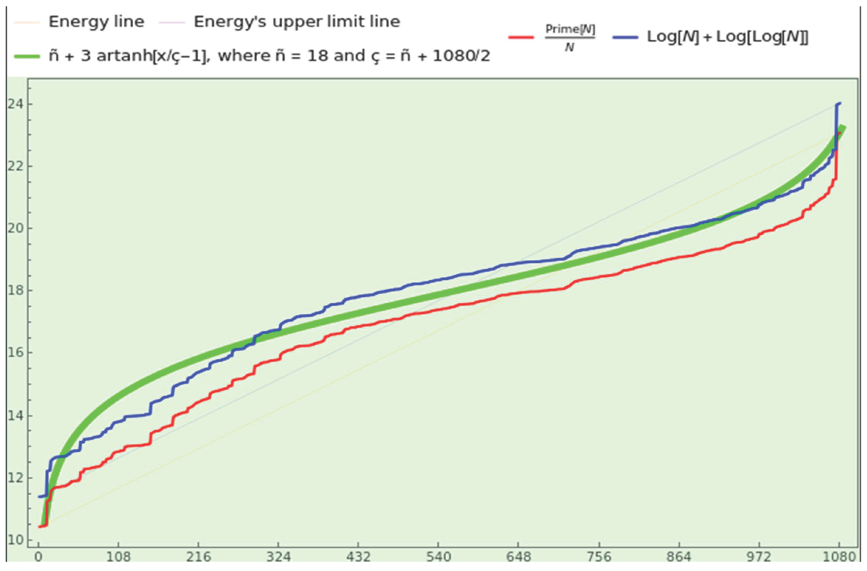
8.2.3. First Characteristic Values of WP
WP contains 57 primes, of the entries. This data is not relevant.
WP produces a split and -equilibrium regarding the rough/smooth balance, very close to the theoretical and values for the naturals. In this regard, WP offers sheer naturalness.
Take, say, the element . Then the SPO is 15, the LPO is 985, and the geometric mean ordinal is . Figure 31 in the top-left corner shows the log-plot of the sorted SPOs, GMOs, and LPOs. We must understand the meaning of these curves separately, because the SPO, GMO, and LPO values at a given position generally correspond to different entries in the WP dataset.
The three log-plots might be segments of an artanh curve, like those produced by the factorization of CT. Accordingly, these profiles allow us to identify natural datasets.
The 19-bin log-histograms of SPO, GMO, and LPO at the bottom-left, top-right, and bottom-right of the Figure 11 apparently fit a lognormal distribution, although this circumstance is difficult to determine with accuracy.
8.2.4. Growth of Divisibility
Figure 33 shows the PMF of (top-left) and the distribution of (bottom-left) for the WP elements, along with the corresponding log2-plots of the sorted omega values (at the right). The histograms depict a lognormal distribution, as do the natural numbers, which reveals the naturalness of the WP dataset. We cannot recognize an artanh curve based on the logarithm of the values of WP, while the growth profile of as an artanh curve segment is definitely an indicator of naturalness.
Expression (7) is obviously true for the elements of WP, i.e., for all , . Interestingly, is very close to the natural asymptotic limit . In this sense, because of its larger size, WP is more organic than CT.
Figure 34 shows the distribution of (top-left) and (bottom-left) for the entries of WP, along with the corresponding logarithmic plots. The histograms depict a hyperbola, just as the natural numbers do, which reveals the naturalness of the WP dataset. We cannot infer information from the logarithm of the values of WP, while the artanh growth profile of is definitely an indicator of naturalness.
Figure 15 at the bottom shows the growth of the average sum of the number of divisors rendered by the WP entries. Although an incipient segment of artanh appears when we use the appropriate radius for the smoothing normal kernel, we cannot take these plots as a reference for naturalness.
Figure 35 shows the distribution of the highly composite numerals (top-left) and the log10-plot (top-right) of the highly composite counting function of WP (top-right). The histogram depicts a Gaussian distribution, and the plot shows a segment of the artanh function around the straight line joining the minimum and maximum values. The artanh growth profile of the logarithm of the highly composite counting function indicates that we can use this criterion to assess whether a dataset is organic, provided it has more than 1000 entries.
8.2.5. Growth of Primality
Figure 35 shows the distribution of the primes (bottom-left) and the log10-plot (bottom-right) of the prime counting function of WP elements. The histogram depicts a hyperbola, and the log-plot a segment of artanh around the straight line joining the minimum and maximum values. Note that the growth of energy (see Figure 30) is even with the logarithmic growth of the primes. However, the artanh growth profile of is an indicator that a dataset is organic only if it has more than 1000 entries.
The Chebyshev functions yield the interval
inherently associated with the WP’s information. The quotient between them, namely , does not approach that obtained for the WP size (), and therefore, indeed, we cannot take it as a measure of naturalness.
Now, let us calculate the WP-prime counting function. Sort the elements as the sequence and count the number of primes in the sequence less than or equal to every . Since the last element of is 1311050527, then is the number of primes in WP. For example, the first 27 elements of the prime counting function within WP are
because the numerals 10079 at the 7th position and 31319 at the 27th position are the first two primes within WP. Note that .
The plot of appears in Figure 36 (in red) and grows proportionally to (in black), meaning that the WP-prime counting function behaves like for natural numbers. This profile is another indicator of naturalness for a dataset.
8.2.6. Density of Primes
We calculate (see Figure 37) the density of prime ordinals generated by the factorization of WP normalized to the 10th (top-left), 96th (top-right), 1000th (bottom-left), and 10000th (bottom-right) ordinal, respectively. The obtained PMFs comply with the law 3, hence (14), with notable compliance and decreasing RRMSE. In particular, the density of ordinals normalized to the 96th ordinal passes the goodness-of-fit test, with the null hypothesis that the WP follows the law and the alternative hypothesis that they do not fit together.
As for the compliance with the possibilistic law of the minor prime 4, the RRMSEs between the empirical and theoretical distributions normalized to the 20th, 200th, and 2000th ordinals are , , and , respectively.
Consequently, WP is natural with respect to the density of primes. This measure is undoubtedly a strong indicator of a dataset’s naturalness.
8.2.7. SPO Density
We calculate (see Figure 38) the density of prime ordinals at the first position of the SOE representation, i.e., the distribution of SPOs resulting from the factorization of WP normalized to the 3rd (top-left), 10th (top-right), 24th (bottom-left), and 96th (bottom-right) ordinal, respectively. The obtained PMFs adhere to the law 5 with excellent RRMSE. In particular, the SPO density normalized to the 96th prime ordinal passes the goodness-of-fit test, with the null hypothesis that the WP sticks to the law and the alternative hypothesis that they do not fit together.
Hence, WP is natural concerning the density of the SPOs, another strong indicator of the extent to which a dataset is natural.
8.2.8. LPO Density
Factorize WP and calculate the distribution of ordinals appearing at the last place of the SOE representation. The plot of the LPO distribution is as irregular as that of CT and broader, spanning a wide range from 3 (the 2nd prime) to 65755428 (the 5210186th prime). For the first 12 ordinals the sequence of occurrences is , meaning that we have no entry with LPO 1, 2, or 4, one occurrence of 3 and 5, two occurrences of 7, 8, and 11, three occurrences of 6, 8, and 10, and five occurrences of 12. The peak of the LPO distribution is at ordinal 26 (7 occurrences). To smooth the first 400 elements and obtain an approximating function that captures the the WP pattern, we convolved the truncated LPO distribution with a Gaussian filter of radius 25 and then normalize to achieve countable additivity (i.e., unitarity). We show the plot of the resulting PMF in Figure 4, in green; conformance with the natural distribution and the lognormal distribution is again notable, except for ripples in the tail.
Consequently, WP is natural in terms of the LPO density, and this profile is another strong indicator of naturalness.
8.2.9. k-Almost Primes and Interaction
We calculate
and normalize it to 1 to satisfy countable additivity. We cannot compare the resulting PMF with that obtained from the law 6 in absolute terms, but its logarithm shows a nearly straight line, as shown in Figure 20 (in gray). This fact means that the logarithmic profiles corresponding to the first law of the least interactors generated by (see Figure 20, in blue) and WP are similar if we disregard the scale factor.
We also calculate
and normalize to one. We cannot compare the resulting PMF with that obtained from the law 7 in absolute terms, but its logarithm shows a nearly straight line, as shown in Figure 20 (in orange). The logarithmic plots corresponding to the second law of the least interactors generated by (see Figure 20, in red) and WP are similar if we disregard the scale factor. Moreover, the WP logarithmic profiles of the first and second laws are nearly superimposed and are definitely typical of natural datasets, much as the NBL.
WP displaces the peak of pairwise interactions to the 3-almost primes (those natural numbers that are the product of exactly three, not necessarily distinct, prime numbers). However, for the rest of the interactions (), the 4-almost primes are protagonists, even after applying a normal smoothing filter of radius 3 to the almost-prime zeta PMFs (see Figure 39, top-left). We can approach the PMF for the range of k-almost primes only by means of a generalized gamma distribution [63] using shape parameters 0.46 and 2.75, scale parameter 6, and location parameter 0.5 (top-left in gray). Since this profile differs from that of CT, it can serve as an indicator of naturalness only if the dataset contains more than 1000 entries.
Like in the case of the naturals, the tails with for all s are not fat, but decay exponentially (see Figure 39, top-left). Between (s=10) and (s=2) of the WP interactions involve k-almost primes with .
We illustrate the three-dimensional log-plot of the sums in the bottom-right corner of the Figure 39. The z-axis represents the sum’s logarithm as a function of the s-axis and the k-axis. For example, the point
indicates that the logarithmic weight of the 5-almost primes is in WP interactions with 3 participant entries. The reason why the log-maximum of these partial sums, namely , does not coincide with the maximum of this three-dimensional plot is that the latter has interpolation order 3.
The 2-almost primes are the primary interactors among the square-free entries of WP; for example, the PMF for s=4 is . In general, the tails of decay exponentially. For example, the weight of the square-free interactions between 2, 3, and 4 elements of WP due to numbers with 1, 2, or 3 distinct prime factors is 0.92366, 0.96339, and 0.98589, respectively, while the weight of the square-free 6-almost primes is negligible for all the interactions. However, if we apply a normal smoothing filter of radius 3 to the square-free almost-prime zeta PMFs, these become monotonically decreasing functions except for for pairwise interactions (see Figure 40, top-left), like those of . We can model the PMF for the range of k-almost primes only via a generalized gamma distribution with shape parameters 0.38 and 2.8, a scale parameter of 3.7, and a location parameter of 0.5 (top-left in gray). Since this profile differs from that of CT, it can serve as an indicator of naturalness only if the dataset contains more than 1000 entries.
We illustrate the three-dimensional log-plot of the sums in the bottom-right corner of the Figure 40. For example, the point
indicates that the logarithmic weight of the 5-almost primes is with respect to WP square-free interactions with 3 participant entries. The reason why the log-maximum of these partial sums, namely , does not coincide with the maximum of this three-dimensional plot (labeled) is that the latter has interpolation order 3. Note that the surface depicted by WP is similar to that of CT, with the key difference being that the CT surface is positioned lower than the WP one. Therefore, we can take this 3D profile of the log-plot of the square-free almost primes as another sign of naturalness.
Another characteristic of WP that shares with is that the logarithmic plot of the k-almost prime zeta functions, square-free or not, slightly warps regarding the straight line that joins the first and last points of every PMF the interaction laws produce (see Figure 39 and Figure 40, top-right). We find the bulk of flex points at s=4 for the general and square-free k-almost prime zeta function PMFs when we discard eleven or more interactors. The warp along the k-axis is more irregular (see Figure 39 and Figure 40, bottom-left). Because the logarithmic profiles of the k-cuts rendered by CT and WP are similar, we can use them as indicators of naturalness, expecting the flex point to be closer to s=2 as the dataset size increases.
8.2.10. Totatives
The logarithm of the WP totatives spans an artanh segment between the first and last elements (see Figure 41, top-left). This profile characterizes the natural datasets with more than 1000 numerals.
Sort the entries of the WP dataset and calculate its intratotatives. The rate intratotatives/non-intratotatives for the WP dataset is ; we calculate the numerator as the amount of intratotatives (323484) divided by , where 1080 is the cardinality of the dataset in hand, and we calculate the denominator as the total of non-intratotatives (260256) minus the size of WP (to exclude the cases where any number is divisible by itself). Note that 0.5552 is the empirical probability of the WP pairwise irreducibility, a figure that is not far from that of the naturals, namely (a gap of about ), and can also be helpful to characterize an organic dataset.
The plot of these intratotatives (see Figure 41, top-right) and non-intratotatives (see Figure 41, bottom-left) replicates the lower and upper limits of growth of the natural line. The intratotative proportionality constant of WP is , i.e., a lower bound that guarantees that the nonzero intratotative values fulfill for those . The non-intratotative proportionality constant of WP is , i.e., an upper bound that guarantees that intratotative values fulfill for those . To satisfy this pair of constraints, we exclude the first few elements, say 5, where the totient function behaves erratically.
As for the average growth of WP intratotatives, we have obtained a straight line, as the theory of natural numbers predicts. The rate of growth with respect to that of (see Figure 41, bottom-right) is
A gap value below is plausibly enough to avoid rejecting WP as natural.
Because the totatives focus on pairs with GCD=1, we have extended the study also to handle pairs with any GCD. We show the distribution from GCD 1 to 15 obtained from the pairwise processing of WP in Figure 42, top-left. The masses of the law of the minor GCD (proportional to ) and the empirical GCD masses resulting from the processing of WP are notably close (see Figure 42, top-right). Then, we performed a goodness-of-fit hypothesis test, obtaining p-values close to 1 (see Figure 42, bottom-left), suggesting that we cannot reject the null hypothesis that the PMFs have the same distribution. Likewise, we have produced a probability-probability plot of the two cumulative distribution functions (see Figure 42, bottom-right) to confirm that the theoretical and empirical PMFs are nearly identical
Moreover, the skewnesses of the WP-empirical and -theoretical GCD plots are 3.045 and 3.13, respectively. The kurtosis of the WP PMF is 11.018 and the kurtosis of the law’s PMF is 11.482. The RRMSE of the empirical dataset relative to the law is about 1.9, indicating excellent agreement.
The key takeaway is that WP is a ” natural” dataset for GCD frequencies.
8.2.11. Density of Divisors
We factorize WP, group by prime factors with multiplicity, and calculate the PMF for the first 12, 120, 1200, and 12000 ordinals. Then, we calculate the PMF of the corresponding law, namely 9, for the first 12, 120, 1200, and 12000 ordinals. Both PMFs approach each other with RRMSE values of , , , and , respectively. The gap between the empirical and theoretical first masses is , , , and , respectively. In Figure 43, we show the first 12 frequencies for both PMFs to compare the empirical (red) and theoretical (blue) densities.
Likewise, we have calculated the corresponding possibility distribution function (maximum membership degree one) by dividing the distribution of occurrences by the maximum value, which corresponds to . In Figure 44, we show the density of divisors with multiplicity yielded by the factorization of WP (red plot) in comparison with the theoretical frequency relative to . The similarity between the two plots is excellent, as confirmed by the RRMSE. Hence, WP, like CT, obeys the law 10, which indeed characterizes the natural datasets.
8.2.12. Density of Exponents
We display the distribution of exponents in the top-left corner of Figure 45. The frequencies of the general law of the minor exponent and the exponents obtained from the WP factorization, which reach the eleventh power, are practically indiscernible (see Figure 45, top-right). The goodness-of-fit hypothesis test (see Figure 45, bottom-left) suggests that we cannot reject the null hypothesis that the datasets have the same distribution, against the alternative that they do not fit. Likewise, the probability-probability plot of the two cumulative distribution functions (see Figure 45, bottom-right) indicates that the two datasets closely agree.
Moreover, the skewness of the WP exponents and the law exponents are 2.766 and 2.769, respectively. The kurtosis of the WP exponents and that of the law are 8.814 and 8.821, respectively. The RRMSE statistical test, which computes a normalized measure of the average absolute difference between the empirical and expected masses, yields a value of , indicating almost exact conformity.
8.2.13. Density of the LPE
The LPE distribution reaches the eleventh power (see Figure 46, top-left). The frequencies of the law of the LPE and the LPEs obtained from the WP factorization are very close (see Figure 46, top-right). The goodness-of-fit hypothesis test (see Figure 46, bottom-left) suggests that we cannot reject the null hypothesis that the datasets have the same distribution, against the alternative that they do not fit. Likewise, the probability-probability plot of the two cumulative distribution functions (see Figure 46, bottom-right) indicates close agreement.
Moreover, the skewness of the WP LPEs and the law of LPEs are 1.66 and 1.72, respectively. The kurtosis of the WP LPEs and the law of LPEs are 4.37 and 4.55, respectively. The RRMSE of the empirical LPE of WP with respect to the law is about , implying excellent conformance.
Consequently, WP is a ” natural” dataset from the LPE perspective.
9. Concluding Remarks
Let us take stock of this document, which aims to analyze the number-theoretic underpinnings of the prime factorization of unprocessed numerical data samples, including subsets of the natural numbers.
” For reasons that nobody understands, the universe is deeply mathematical,” says Steven Strogatz. He adds, ” There seems to be something like a code of the universe, an operating system that animates everything from moment to moment and place to place.” According to Wheeler, we should ” regard the physical world as made of information” because ” all things physical are information-theoretic in origin, and this is a participatory universe.” The information managed by such a universal code would be numeric, suggesting that numbers are not merely lifeless symbols but rather integral to living things, as Benford remarked in the closing sentences of his article.
A critical observation is that the physical information we receive is seldom linear. NBL indicates that the minor digits occur more frequently than the significant digits. Since digits represent numbers and numbers convey information, we can infer that the cosmos maintains an entropic balance by presenting numerous elements of low informational value alongside a few of high informational value. Then, how is information organized? Furthermore, should we not recognize this pragmatic preference for frugality in the canonical factorization of a raw numerical dataset as a bias towards minor prime power factors?
The informational representational cost of a natural N is proportional to its energy , which grows as . Based on the idea of resource economy, nature likely first considers the ” price” of the operands before proceeding with the subsequent calculations. For example, accurately adding numbers that differ by no more than two orders of magnitude makes sense. However, the efficiency of accurately summing 2 to () is questionable. Consequently, the logarithm of a numeral (or its harmonic number) is either explicitly incorporated in its representation or implicitly expressed by the number of prime factors. In this case, some form of the canonical factorization of the naturals might be ” real” .
The SOE representation introduces a subtle difference from the canonical factorization representation. Both share many advantageous properties, including compactness and scale invariance, due to the explicit form of the exponents. Functions like omega ( and ) and sigma divisors ( and ) are easily computable, and the prime and totative counting functions are tractable. However, the SOE representation emphasizes ordinals rather than the primes themselves. Many of our proposed rules pertain to prime ordinals; by making their accessibility straightforward, we can handle elemental information of practical character.
We have also reviewed the growth of divisibility through the average sum of divisors and the average sum of the sum of positive divisors functions. In this context, the concept of a highly composite number is noteworthy. The abundant composition scale progresses less steeply than the primality scale. The primes, governed by the prime number theorem, share a growth order with the logarithmic integral function, the quotient of sums of divisors, and the Chebyshev functions, allowing us to regard the prime counting function as a quantum energy level on average.
We describe the meaning of a quantum in Section 4. The PMF that states the probability of a nonzero integer Z as allows us to explain that probability is normalized representational information and to derive the harmonic NBL and the standard NBL. The logarithmic scale is local, relating more to our perception than to the actual production of information generated from the global harmonic scale. Moreover, the canonical PMF links directly or indirectly to all the factorization laws we have addressed. For instance, the law of the minor prime (3) is equivalent to the probability of a quantum with a specific base (14); a quantum and a prime constitute the same computational entity. Likewise, the law of the minor GCD (8) and the canonical PMF are essentially the same declaration.
The table below presents a comprehensive set of laws concerning the prime factorization of natural numbers. The law of the minor energy (first row) highlights the connection to the notion of likelihood and the prominence of the lowest informational entities. The law of the minor pairwise GCD (second row) and the possibility law of the minor prime disregarding multiplicity (third row) are well-known. The last nine rows of the table address the probability of a prime disregarding multiplicity within the factorization set, the probability and possibility of the SPO, the number of participants in an interaction (considering or not multiplicity), the probability and possibility of a prime power divisor, the probability of an exponent, and the probability of the LPE. Laws 3, 5, 11, and 7 disregard multiplicity, whereas 6, 9, 10, 12, and 13 consider multiplicity. These nine PMFs, unpublished to our knowledge, serve to illuminate the central idea that the natural preference for the small intensifies in the primality frequency; the smallest primes cover more ground in relative terms than that assigned by NBL to the smallest digits.
| Law of the minor ... | Description | Limiting value |
| Energy of a quantum (law 1) | ||
| Pairwise GCD (law 8) | ||
| Prime relative to the factorized numbers (law 4) | (possibility) | (possibility) |
| Prime relative to the factorization set (law 3) | ||
| SPO (probabilistic law 5) | ||
| SPO (possibilistic law 11) | (possibility) | (possibility) |
| Number of interactors considering multiplicity (law 6) | ||
| Number of interactors disregarding multiplicity (law 7) | ||
| Prime divisor relative to the factorization set (law 9) | ||
| Prime divisor relative to the factorized numbers (law 10) | (possibility) | (possibility) |
| Exponent (law 12) | ||
| LPE (law 13) |
We have conducted an in-depth analysis of a pair of datasets that we see as archetypal examples of non-manipulated data, expecting the lessons learned to be generalizable to any natural dataset. We have reassured ourselves that NBL and CT, as well as NBL and WP, are aligned. The fact that we cannot reject NBL-conformance is good news, given the size of these samples, which contain 300 and 1080 numerals, respectively. However, CT is not only thinner but also more fabricated than WP. The fact that the CT dataset has 8 SPEs greater than 1 () indicates that it has been manipulated to some degree, as natural datasets typically have a much lower percentage, according to our experience. Let us say that CT is a repository of quasi-random numerals. In contrast, WP is a repository of mere raw numerical data.
The information gathered from our observations suggests several conditions for assessing the naturalness of a dataset. Among these requirements, several refer to a generic dataset DS. The requirements marked with an asterisk apply only to datasets of considerable size, specifically those with more than 1000 entries. Criteria involving the symbol of approximation ”≈” lead to avoiding rejection if the error is below .
| Criterion | Description |
| NBL conformance | The PMF of the first digits obeys (16) |
| Informational energy | Growth profile of is an artanh curve segment |
| Growth of the summatory of the prime factors ordinals | Growth profile of is an artanh curve segment |
| Odds of the rough against smooth numbers in DS | |
| Rough/smooth equilibrium in DS | to hold = |
| Growth of SPOs, GMOs, and LPOs | Log-growth profile of these curves is an artanh curve segment |
| Distribution of the omega functions * | The PMFs of and obey a lognormal distribution |
| Growth of the number of prime factors with multiplicity | Growth profile of is an artanh curve segment |
| Difference between the omega functions of DS | , where is the size of DS |
| Histograms of the divisor functions | The histograms of and outline an hyperbola |
| Growth of the sum of divisors function * | Growth profile of is an artanh curve segment |
| Growth of the highly composite counting function * | Log-growth profile of highly composition is an artanh segment |
| Comparison between the growths of energy and primes | Growths of of and are even |
| Growth of the prime counting function * | Growth profile of is an artanh curve segment |
| Growth of the DS-prime counting function | Growth profile of proportional to |
| Criterion | Description |
| Distribution of primes | The PMF of the primes obeys law 3 |
| Distribution of the SPOs | The PMF of the SPOs obeys law 5 |
| Distribution of the LPOs | The PMF of the LPOs obeys a lognormal distribution |
| k-almost DS-prime zeta functions * | profile is like that of Figure 39, top-left in gray |
| Square-free k-almost DS-prime zeta functions * | profile is like that of Figure 40, top-left in gray |
| k-warps of the 3D DS-prime zeta function values | The plot of form an arch when k is fixed |
| Growth of the Euler’s phi (or totient) function * | Growth profile of is an artanh curve segment |
| Rate of DS intratotatives | |
| Growth constant of DS intratotatives | |
| Growth constant of DS non-intratotatives | |
| Average growth of DS intratotatives | grows as the straight line , where |
| Distribution of the pairwise GCD | The pairwise GCD PMF obeys law 8 |
| Distribution of divisors with multiplicity | The PMF of the prime divisors weighted by the exponent obeys law 9 |
| Relative frequency of divisors with multiplicity | The possibility of the prime divisors weighted by the exponent obeys law 10 |
| Distribution of the prime exponent | The PMF of the prime exponents obeys law 12 |
| Distribution of the LPE | The PMF of the LPE obeys law 13 |
All these guiding principles converge on betting for the minor numbers. In general, an ordered set situates the most probable elements close to the origin, while the rare elements are far from the origin. The element of surprise of these hefty numbers counters the fact that, on average, they are level, anodyne, and predictable. The natural (unstable and perturbable) equilibrium is feasible by balancing many small likely elements with a few large unlikely ones.
In light of our findings, the lognormal distribution is a widespread phenomenon. For instance, does there exist a general distribution of a discrete random variable associated with the number of distinct prime factors? Yes, the lognormal distribution. Does there exist a general distribution of a discrete random variable associated with the k-almost primes, square-free or not, for a given number of participants in an interaction? Yes, the lognormal distribution. However, the lognormal distribution is not a panacea. We cannot fit the PMF of the k-almost prime zeta functions to the lognormal distribution for specific natural samples (see Figure 21, Figure 39, Figure 22, and Figure 40 at the top-left). The most we can do to approach such profiles is to utilize the so-called generalized gamma distribution, with four parameters.
An LFT requires precisely four parameters. Since we can express the logarithm of an LFT in terms of the artanh function, an artanh distribution fits all the plots we display in this article. Because an LFT becomes a linear map when its denominator is one, the artanh distribution contains the lognormal one. Curve segments of artanh approach linearity, exponential or logarithmic growth, and exponential or logarithmic (decelerating) decay with the appropriate displacement, rotation, inversion, and scale. Further, the importance of artanh lies in its role as the protagonist function of the conformal 1-ball model, which explains the information-preserving mapping between the external harmonic world and our internal logarithmic world.
The laws we have reviewed or disclosed, as well as the analysis of the empirical results, point to a latent endurance strategy. Concerning the outcomes of natural selection, John David Barrow in ” Pi in the Sky” claims that ” Their primary characteristic is persistence, or stability, rather than simplicity.” By weighing many lighter (or shorter) things against a few heavier (or longer) ones, the universe rejects uniformity in favor of dynamism, not only for rising stability but also for operability as a form of survival. Permanence, regularity, calculability, and balance between homogeneity and heterogeneity are inherent, ubiquitous values that nature fosters to guarantee evolution.
Assuming that nature is prone to managing small significands, one can infer an endemic preference for the minor primes, too. However, this affirmation needed supporting evidence. The primality setting we have focused on demonstrates that, for instance, number one appears most frequently as the leading prime ordinal and exponent, and the probability mass for two, three, etc., as ordinal and exponent, decreases significantly. Large ordinals are not common. High exponents are extremely occasional. We conclude that SOE is plausibly a fundamental representation, that the laws of the minor primes rule the natural datasets, and that the prevalence of the small over the large, at proper proportions, constitutes a tenet of the cosmos’ behavior.
10. Postscript
This apopemptic chapter includes additional information about the context of our activity during the article’s development.
Data Availability Statement
This article includes original contributions. Readers can contact the author for further inquiries. The programming code used to generate the data presented in this study is available upon request.
Acknowledgments
We hereby express our tribute to the personalities and entities that have influenced this work. The UNED instilled a scientific instinct and a generalistic approach to problem-solving. Working for Indra enabled a pragmatic approach to addressing crises and an awareness of the productive character of our universe. We greatly thank José Mira for his motivational capacity. We apologize in advance for omitting laudable references. We sincerely appreciate those who offer comments and critical insights on this version.
Conflicts of Interest
This research received no external funding. Therefore, the author (ORCID 0000-0003-3980-5829) declares no conflicts of interest. The author asserts that only scientific rigor, significance, and clarity drive the work’s high-level goals. It contains no known minor or significant incongruities, errors, or inaccuracies. The author did not receive support from any organization for the submitted work and declares that he has no competing financial or nonfinancial interests directly or indirectly related to the work submitted for publication. No personal relationships have influenced the content of this work. It has not been published elsewhere in any form or language, in whole or in part. The author claims to have committed no intentional ethical wrongdoing related to this paper, including self-plagiarism, plagiarism, far-fetched self-citations, conflict of interest, inaccurate authorship declarations, and unacceptable biases concerning the references. This work respects the rights of third parties, including copyright and moral rights.
Abbreviations
| (in alphabetical order) | |
| GCD | Greatest Common Divisor |
| LFT | Linear Fractional Transformation |
| LPE | Largest Prime Exponent |
| LPO | Largest Prime Ordinal |
| NBL | Newcomb-Benford Law |
| PMF | Probability Mass Function |
| RRMSE | (Relative Root Mean Squared Error) |
| SOE | Standard Ordinal-Exponent representation |
| SPE | Smallest Prime Exponent |
| SPO | Smallest Prime Ordinal |
References
- Wikipedia contributors, the Free Encyclopedia. Positional Notation, 2022. [Online; accessed 11-November-2022].
- Arno Berger and Theodore P. Hill. What is Benford’s Law? Notices of the AMS, 64(2):132–134, 2017.
- Arno Berger and Theodore P. Hill. An Introduction to Benford’s Law. Princeton University Press, 2015.
- Eric (https://math.stackexchange.com/users/259049/eric). The prime numbers do not satisfies Benford’s law. Mathematics Stack Exchange, 2015. URL:https://math.stackexchange.com/q/1385292 (version: 2015-08-05).
- Cohen, D.I.; Katz, T.M. Prime numbers and the first digit phenomenon. J. Number Theory 1984, 18, 261–268. [CrossRef]
- Chris Caldwell. Does Benford’s Law Apply to Primes? PrimePages, 2021.
- J. P. Serre. A Course in Arithmetic. Graduate Texts in Mathematics. Springer New York, 2012.
- Luque, B.; Lacasa, L. The first-digit frequencies of prime numbers and Riemann zeta zeros. Proc. R. Soc. A: Math. Phys. Eng. Sci. 2009, 465, 2197–2216. [CrossRef]
- Alex Ely Kossovsky. Prime Numbers, Dirichlet Density, and Benford’s Law, 2016.
- Wikipedia contributors, the Free Encyclopedia. Erdos-Kac Theorem, 2024. [Online; accessed 23-August-2025].
- G. H. Hardy, E. M. Wright, R. Heath-Brown, J. Silverman, and A. Wiles. An Introduction to the Theory of Numbers. Oxford mathematics. Oxford University Press, 2008 (1938).
- Julian Havil. Gamma - Exploring Euler’s Constant. Princeton University Press, 2003.
- Steven R. Finch. Mathematical Constants. Encyclopedia of Mathematics and its Applications. Cambridge University Press, 2003.
- Mark J. Nigrini. Digital analysis using Benford’s Law. 2000.
- Despotovic, M.; Nedic, V.; Despotovic, D.; Cvetanovic, S. Evaluation of empirical models for predicting monthly mean horizontal diffuse solar radiation. Renew. Sustain. Energy Rev. 2016, 56, 246–260. [CrossRef]
- Werner Stahel and Eckhard Limpert. The Normal Distribution is the Log-normal Distribution. ETH Zürich, December 2014.
- Sen, P.K.; Kagan, A.M.; Linnik, Y.V.; Rao, C.R.; Ramachandran, B. Characterization Problems in Mathematical Statistics. Technometrics 1975, 17, 385. [CrossRef]
- Fang, G.; Chen, Q. Several common probability distributions obey Benford’s law. Phys. A: Stat. Mech. its Appl. 2020, 540. [CrossRef]
- Cerqueti, R.; Maggi, M. Data validity and statistical conformity with Benford’s Law. Chaos, Solitons Fractals 2021, 144. [CrossRef]
- Paul R. McCreary, Teri Jo Murphy, and Christian Carter. The Modular Group. The Mathematica Journal, 20, 2018.
- Rives, J. The Code Underneath. Axioms 2025, 14, 106. [CrossRef]
- Wikipedia contributors, the Free Encyclopedia. Optimal radix choice, 2025. [Online; accessed 25-February-2025].
- Mayne, A.J.; Klir, G.J.; Folger, T.A. Fuzzy Sets, Uncertainty, and Information. J. Oper. Res. Soc. 1990, 41, 884. [CrossRef]
- R. V. L. Hartley. Transmission of Information. The Bell System Technical Journal, 7(3):535–563, 1928.
- Davis, P.J. The Lore of Large Numbers; American Mathematical Society (AMS): Providence, RI, United States, 1961; ISBN: .
- Giovanni Organtini. Is 10 million times 7 equal to 70 million? Level Up Conding by Gitconnected, (2), November 2020.
- Dinur, I.; Kindler, G.; Raz, R.; Safra, S. Approximating CVP to Within Almost-Polynomial Factors is NP-Hard. Combinatorica 2003, 23, 205–243. [CrossRef]
- Pierre Dusart. The Kth Prime Is Greater Than k(ln(k)+ln(ln(k-1))) For k>1. Mathematics of Computation, (68):411–415, 1999.
- Martin Raab and Angelika Steger. "Balls into Bins" - A Simple and Tight Analysis. In Michael Luby, J. D. P. Rolim, and Maria Serna, editors, Randomization and Approximation Techniques in Computer Science, pages 159–170, Berlin, Heidelberg, 1998. Springer Berlin Heidelberg.
- Williams, P.M. Bayesian Conditionalisation and the Principle of Minimum Information. Br. J. Philos. Sci. 1980, 31, 131–144. [CrossRef]
- Eric W. Weisstein. Prime Factorization. MathWorld — A Wolfram Web Resource, 2025.
- Wikipedia contributors, the Free Encyclopedia. Prime signature, 2024. [Online; accessed 1-November-2024].
- Wagstaff, S.S.; Riesel, H. Prime Numbers and Computer Methods for Factorization.. Math. Comput. 1987, 48, 439. [CrossRef]
- David Naccache and Igor E. Shparlinski. Divisibility, Smoothness and Cryptographic Applications, 2009.
- M. Beeler, R. W. Gosper, and R. Schroeppel. HAKMEM. Report 239, Artificial Intelligence Lab of MIT, February 1972.
- Daniel H. Greene and Donald E. Knuth. Mathematics for the Analysis of Algorithms, 3rd edition. Birkhauser, Boston, reprint of the 1990 edition edition, 2008.
- Matt O’Dowd. Can Space Be Infinitely Divided? PBSSpaceTime (Patreon), June 2021. Video.
- L. Alaoglu and P. Erdos. On Highly Composite and Similar Numbers. Transactions of the American Mathematical Society, 56(3):448–469, 1944.
- József Sándor, Dragoslav S. Mitrinovic, and Borislav Crstici. The Arithmetical Function d(N), Its Generalizations and Its Analogues, pages 39–75. Springer Netherlands, Dordrecht, 2006.
- Paulo Ribenboim. The Little Book of Bigger Primes. Springer Nature Book Archives Millennium. Springer Science and Business Media, 2004.
- Albert Edward Ingham. The Distribution of Prime Numbers. Cambridge Mathematical Library. Cambridge University Press, 1990.
- Ruiz, S.M. 81.27 A result on prime numbers. Math. Gaz. 1997, 81, 269–270. [CrossRef]
- Daniel Fischer. Least Common Multiple lim[1,2,…,n]n=e. Mathematics Stack Exchange, June 2014. (version: 2014-06-15).
- Schechter, B.; Hoffman, P.; Lax, P.D. My Brain is Open: The Mathematical Journeys of Paul Erdös and the Man Who Loved Only Numbers: The Story of Paul Erdös and the Search for Mathematical Truth. Phys. Today 1999, 52, 69–70. [CrossRef]
- Wikipedia contributors, the Free Encyclopedia. Coprime integers, 2025. [Online; accessed 2-September-2025].
- George E. P. Box and R. Daniel Meyer. An Analysis for Unreplicated Fractional Factorials. Technometrics, 28(1):11–18, 1986.
- Richard J. Mathar. Series of Reciprocal Powers of k-almost Primes, 2009.
- Mason https://math.stackexchange.com/users/552184/mason. The alternating series of square-free k-almost prime zeta functions converges to the reciprocal zeta? Mathematics Stack Exchange, March 2019. URL:https://math.stackexchange.com/q/2853354 (version: 2019-09-02).
- J. Pettofrezzo and D. R. Byrkit. Elements of Number Theory. Prentice-Hall, 1970.
- Arnold Walfisz. Weylsche Exponentialsummen in der neueren Zahlentheorie. Mathematische Forschungsberichte. VEB Deutscher Verlag der Wissenschaften, 1963.
- H. Q. Liu. On Euler’s function. Proc. R. Soc. Edinburgh: Sect. A Math., 146(4):769–775, 2016.
- Chidambaraswamy, J.; Sitaramachandrarao, R. On the probability that the values of m polynomials have a given g.c.d.. J. Number Theory 1987, 26, 237–245. [CrossRef]
- Roger Tynes. If D is an Integral Domain and has finite characteristic p, prove p is prime. Mathematics Stack Exchange, 2014. URL:https://math.stackexchange.com/q/609982 (version: 2015-11-09).
- Francesco Pappalardi. A survey on k-freeness. In Proceeding of the Conference in Analytic Number Theory in Honor of Prof. Subbarao at IM Sc. Chennai. UniRoma, 2003.
- Burke, J.; Kincanon, E. Benford’s law and physical constants: The distribution of initial digits. Am. J. Phys. 1991, 59, 952–952. [CrossRef]
- R. A. Serway and J. W. Jewett. Physics for Scientists and Engineers with Modern Physics. Number v. 1 in Physics for Scientists and Engineers. Thomson-Brooks/Cole, 2008.
- Wikipedia contributors, the Free Encyclopedia. List of mathematical constants, 2025. [Online; accessed 26-June-2025].
- Wikipedia contributors, the Free Encyclopedia. Gravitational constant, 2025. [Online; accessed 26-June-2025].
- Eric W. Weisstein. Benford’s Law. MathWorld — A Wolfram Web Resource, 2020. [Online; accessed 1-June-2022].
- Wikipedia contributors, the Free Encyclopedia. P-P plot, 2025. [Online; accessed 5-September-2025].
- Wikipedia contributors, the Free Encyclopedia. Log-normal distribution, 2025. [Online; accessed 12-October-2025].
- Sh. T. Ishmukhametov and F. F. Sharifullina. On Distribution of Semiprime Numbers. Russian Mathematics, 58(8):43–48, 2014.
- Wolfram Research. GammaDistribution Function. Wolfram Language and System Documentation Center, page Backgrounf and Context, 2007.
Figure 1.
Log-plot of the sums of the prime factor ordinals for every natural number in the range , where M=2 (top-left), M=3 (top-right), M=4 (bottom-left), and M=5 (bottom-right).
Figure 1.
Log-plot of the sums of the prime factor ordinals for every natural number in the range , where M=2 (top-left), M=3 (top-right), M=4 (bottom-left), and M=5 (bottom-right).
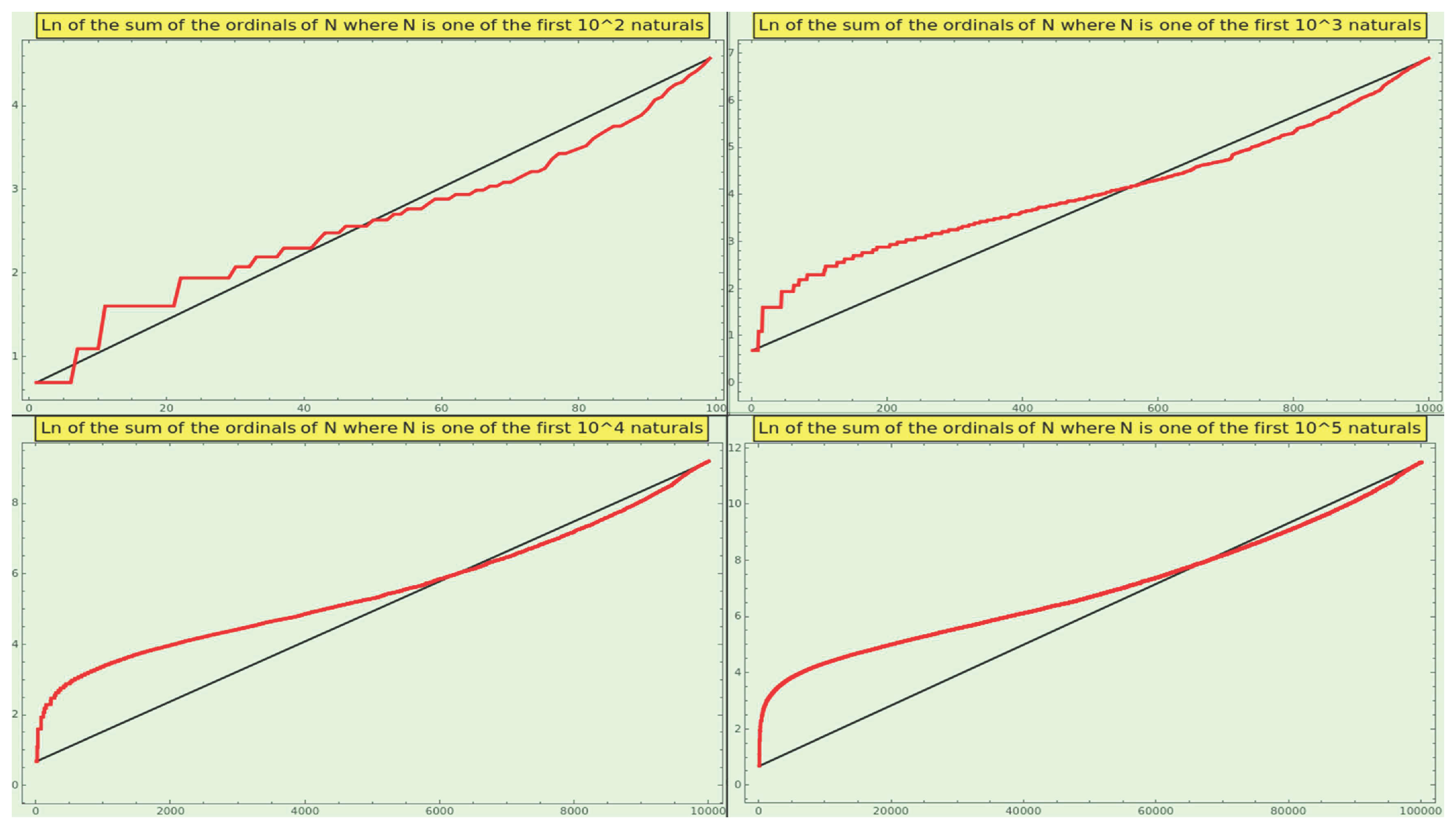
Figure 2.
Plot of the probability masses of the prime factors (disregarding the exponents) resulting from the factorization of the natural numbers between and the Mth prime, where M=10 (top-left), M=100 (top-right), and M=100 (bottom-left). The RRMSE between the empirical data and the data obtained from the definition 3’s formula decreases as M goes to infinity. The x-axis indicates the prime ordinal, o, and the y-axis indicates the occurrence frequency. The plot in the bottom-right corner shows the empirical and expected probability measures for the prime ordinals resulting from the factorization of the natural numbers between and .
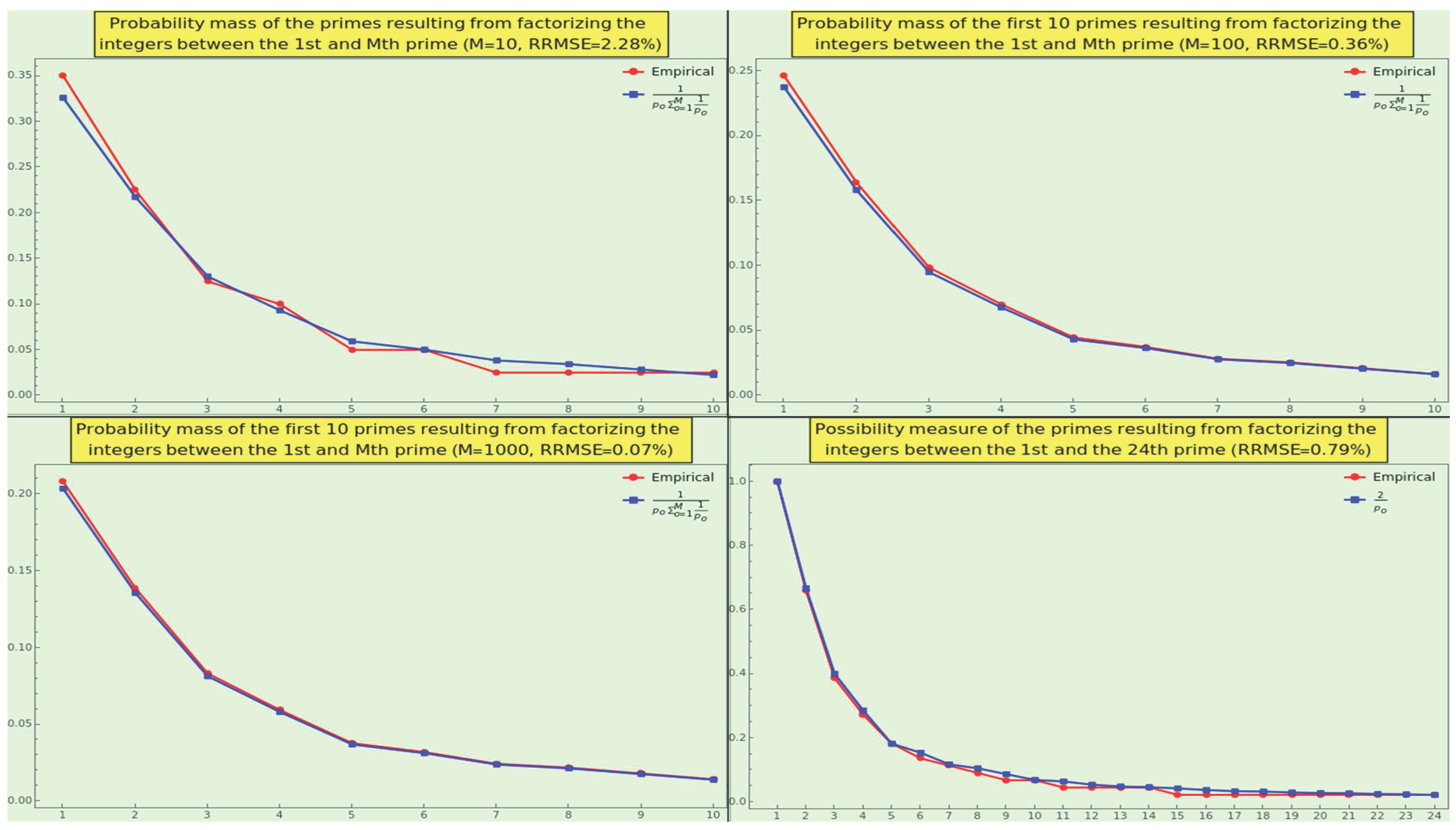
Figure 3.
Take the naturals ranging from 2 to 500000, factorize, and calculate the distribution of the SPOs. Then, normalized for different values of ” the base” , namely 3 (top-left), 10 (top-right), 24 (bottom-left), and 96 (bottom-right). These PMFs adhere to the law 5; in particular, for 3 elements the empirical and theoretical distributions coincide (RRMSE). The x-axis indicates the SPO, and the y-axis indicates the occurrence frequency.
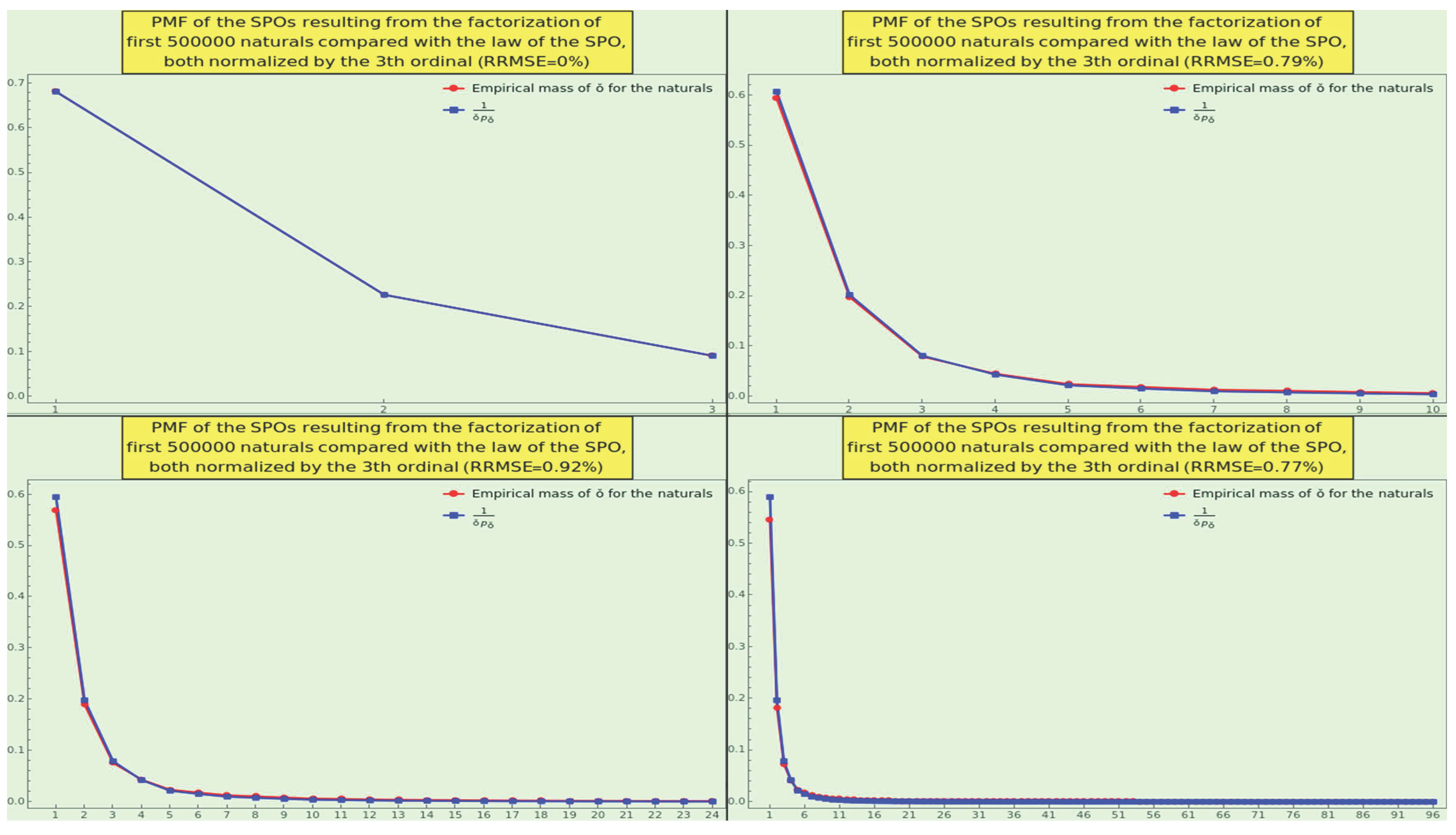
Figure 4.
Take the naturals ranging from 2 to 500000, factorize, and calculate the distribution of the LPOs. Restrict the resulting distribution to a ” base” of 400 ordinals. Repeat the process with the CT dataset, and additionally calculate the convolution with a normal filter of radius 45 elements. Repeat the process with the WP dataset, and additionally calculate the convolution with a normal filter of radius 25 elements. Normalize the distributions of the three datasets (the naturals, CT, and WP) to obtain the corresponding PMFs of LPO. Then, fit the natural PMF to a lognormal model; a mean of 4.32 and a standard deviation of 1.28 yield excellent accuracy with an RRMSE of . Note that the natural PMF and the lognormal model have fat tails, meaning that the PMF decreases algebraically rather than exponentially as we get close to 400. Between the empirical plots of the naturals and CT, the RRMSE is . Between the lognormal model and the empirical CT plot, the RRMSE is . Between the empirical plots of the naturals and WP, the RRMSE is . Between the lognormal model and the empirical plot of WP, the RRMSE is .
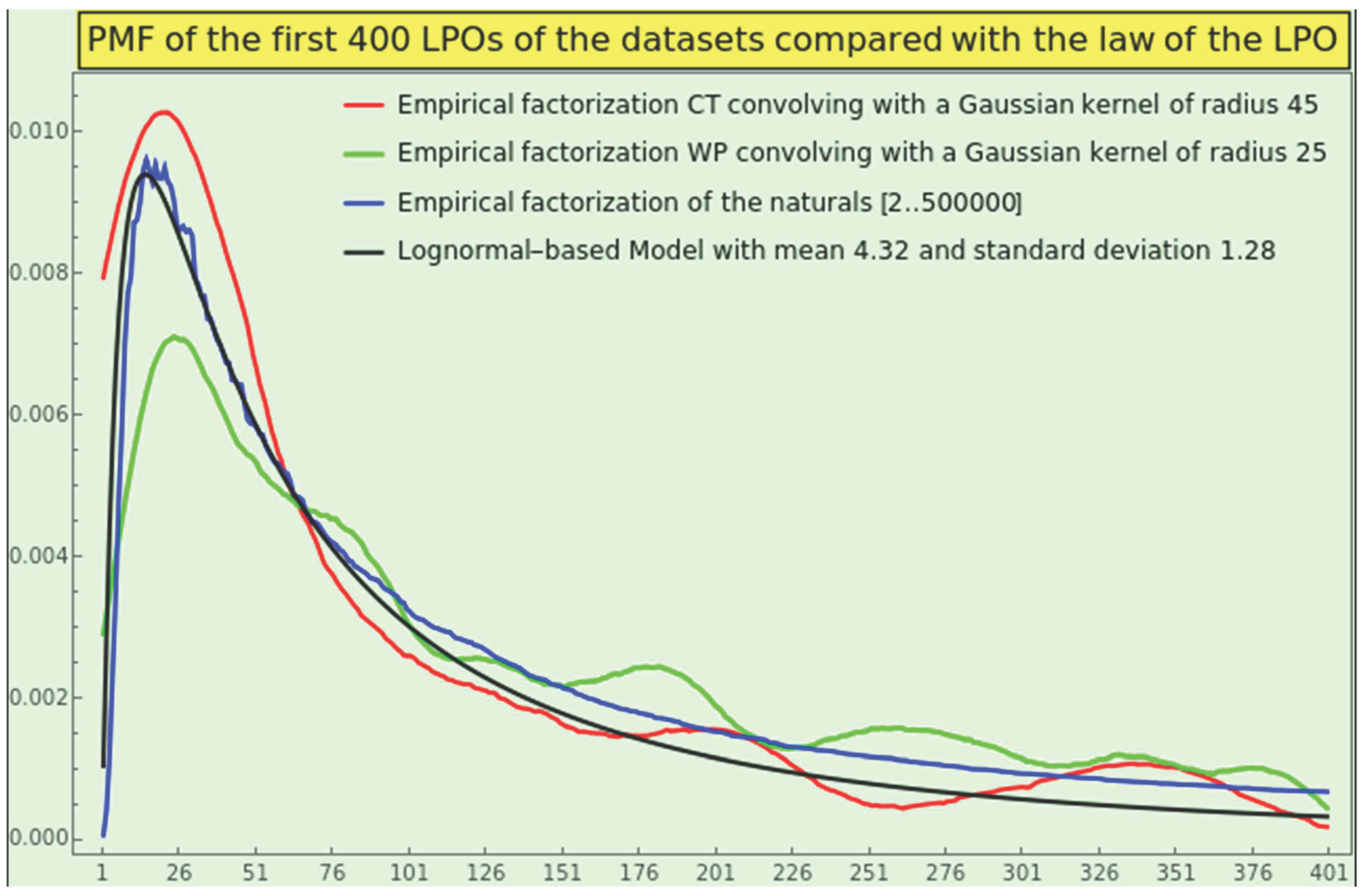
Figure 5.
We illustrate the bias of the natural numbers towards the minor numbers. At the top-left, we show the PMFs of the empirical (in blue), the estimated (in purple) using a lognormal model with log-location 0.1 and log-scale 0.57, the empirical (in red), and the estimated (in orange) using a lognormal model centered at the origin and log-scale 0.45; the probability mass of the square-free almost-primes is negligible if . We show in the top-right corner the PMFs of the first (in blue) and second (in red) laws of interaction from s=2 (pairwise interaction) to s=10 (denary interaction). We also outline in orange (no labels) a lognormal model (log-location 0.135 and log-scale 0.635) that fits both empirical PMFs. We show in the bottom-left corner the log10-plots of the first (in blue) and second (in red) laws of interaction from s=2 to s=26, which practically coincide and exhibit a slight warping. In the bottom-right corner, we show the distance from the log10-plots to the straight line joining the log10-plot at s=2 and the log10-plot at s=10.
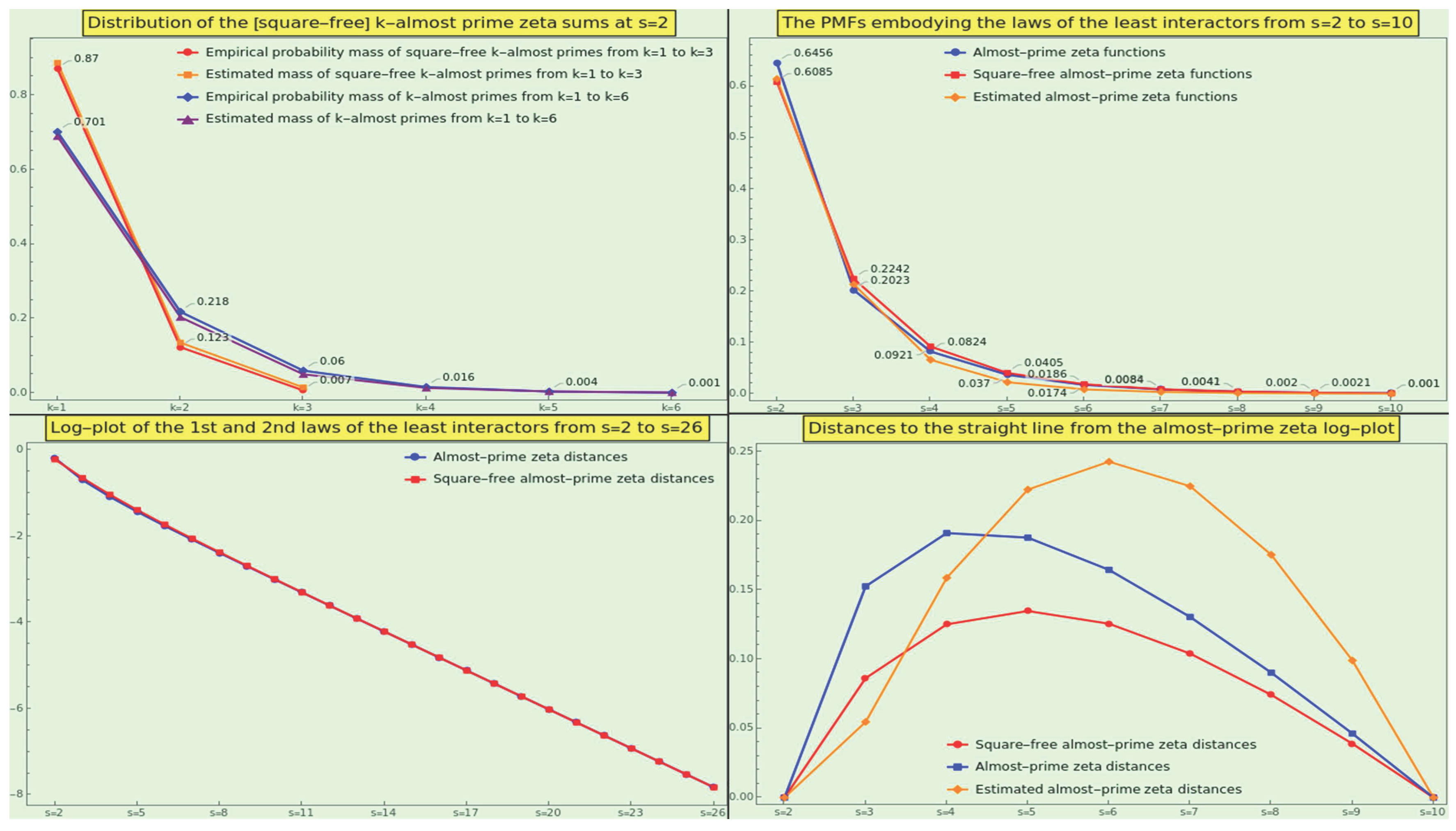
Figure 6.
Plot of the probability mass of the prime divisors (with multiplicity) resulting from the factorization of the natural numbers from up through the Mth prime, where M=10 (top-left), M=100 (top-right), M=1000 (bottom-left), M=10000 (bottom-right). The x-axis indicates the prime ordinal k, and the y-axis indicates the occurrence frequency. The RRMSE between the empirical data and the data obtained from law 9 decreases as M goes to infinity, as does the gap between the first two probability masses 0.06225, 0.04878, 0.0346, and 0.02616, respectively.
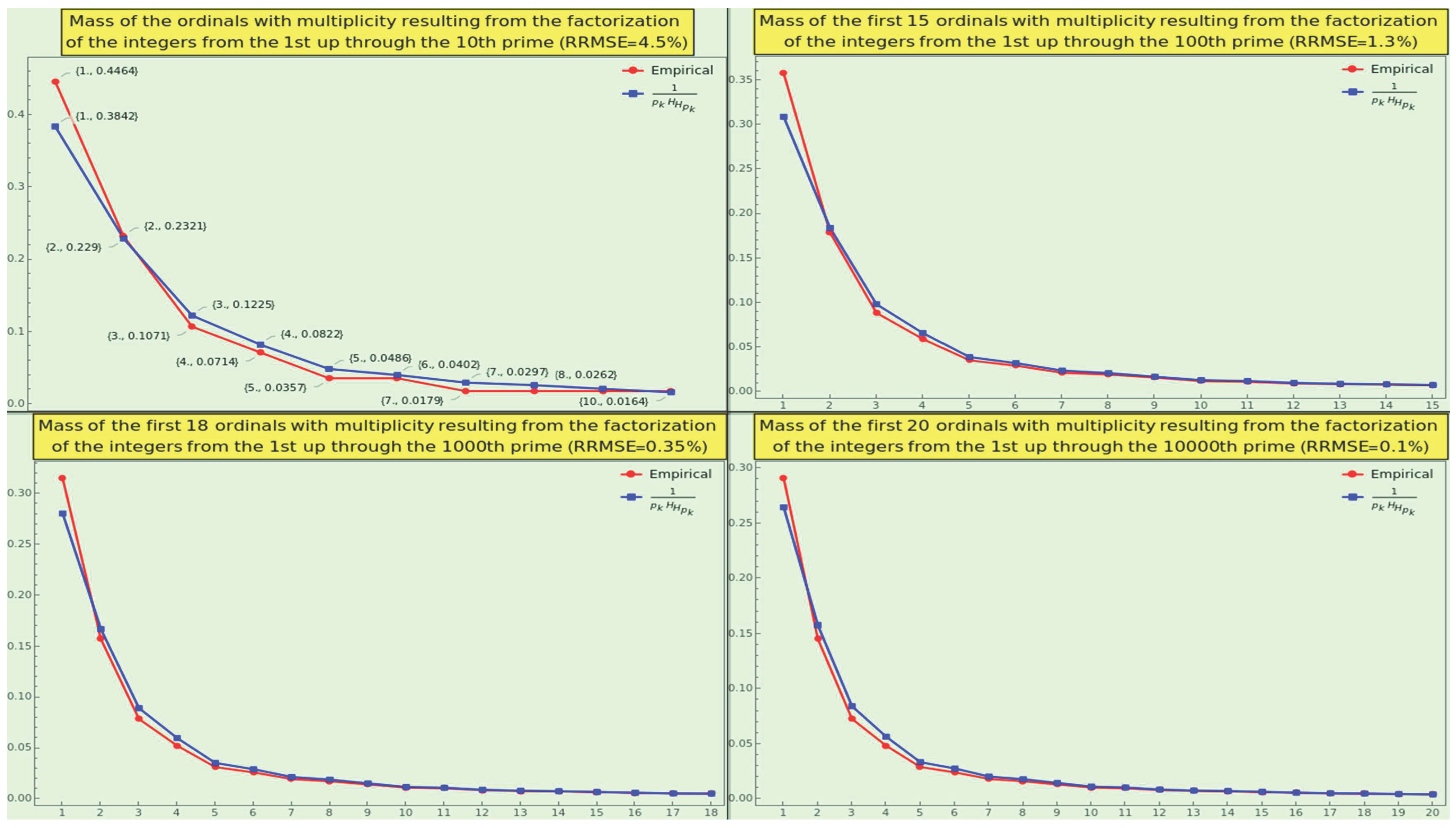
Figure 7.
The factorization of the first th naturals reaches the multiplicity 16. The empirical (in red) and theoretical (law 12, in blue) distributions of multiplicities coincide; the RRMSE is 0.23%.
Figure 7.
The factorization of the first th naturals reaches the multiplicity 16. The empirical (in red) and theoretical (law 12, in blue) distributions of multiplicities coincide; the RRMSE is 0.23%.
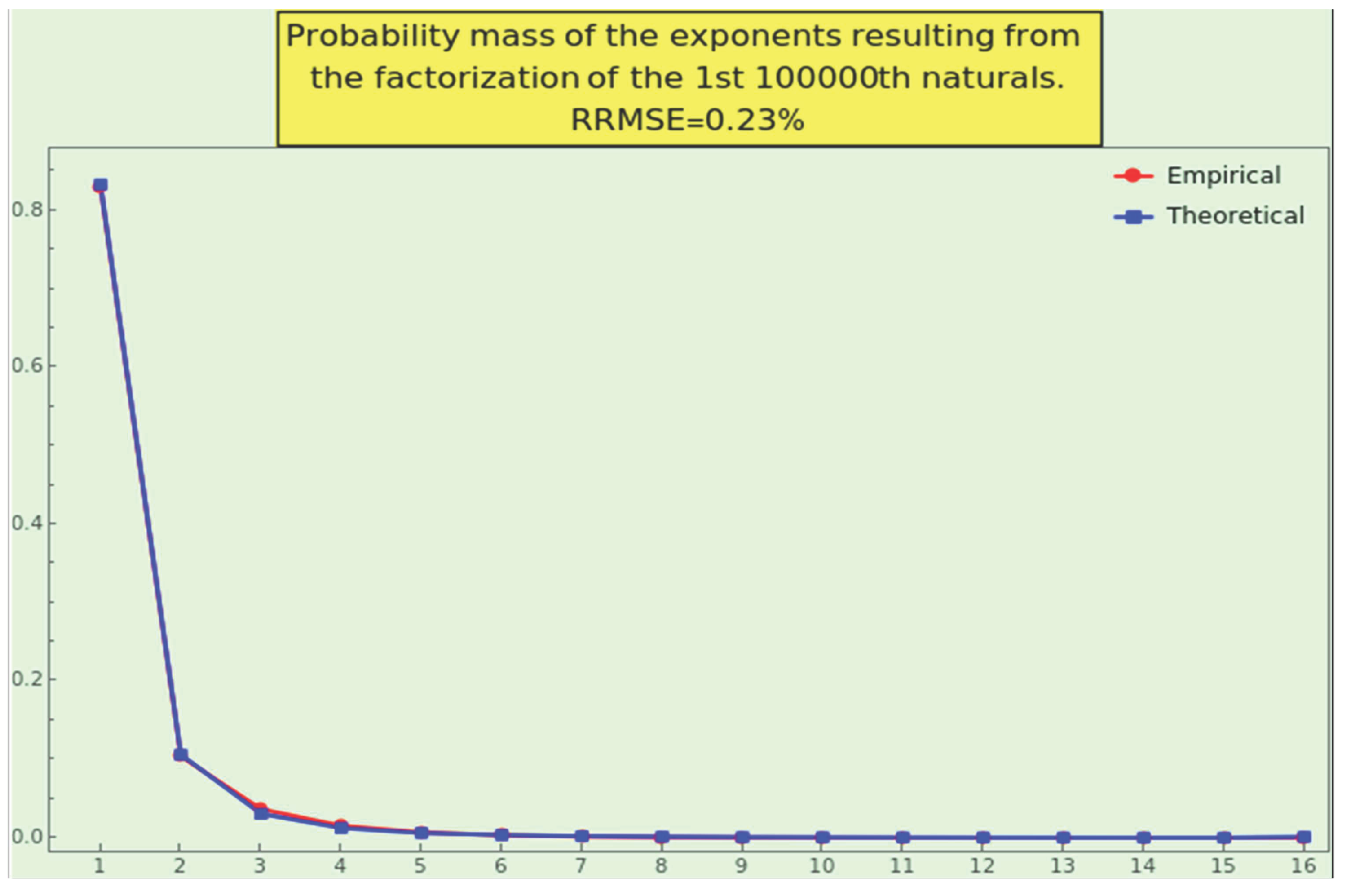
Figure 8.
The prime factorization of the first 500000 natural numbers reaches the multiplicity 18, as indicated by the histogram. The plot of the frequencies (empirical in red and theoretical in blue), the p-values of the statistical tests applied to this factorization, and the P-P plot indicate that the empirical and theoretical PMFs of the LPE are hardly distinguishable.
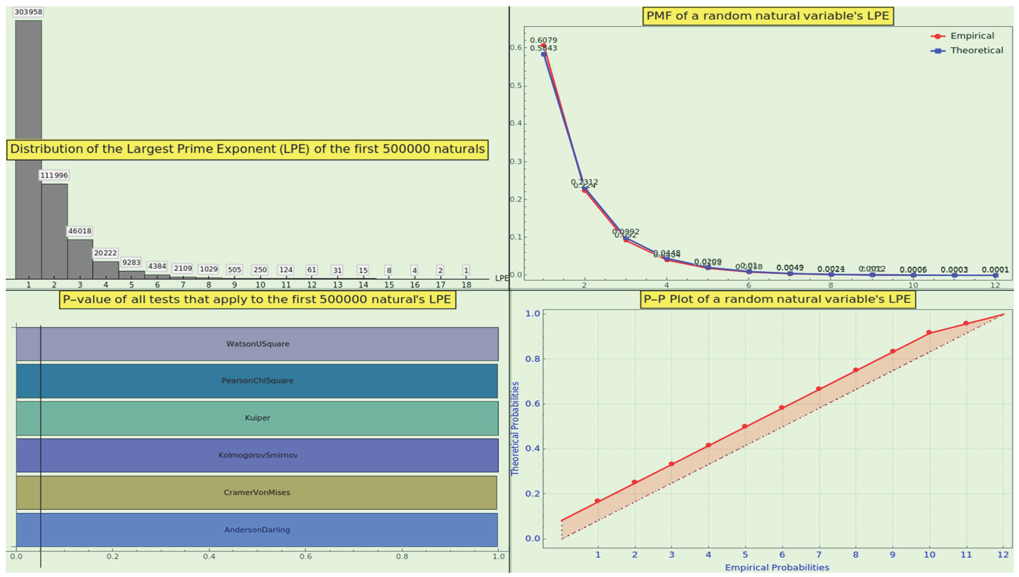
Figure 9.
CT plausibly complies with NBL.
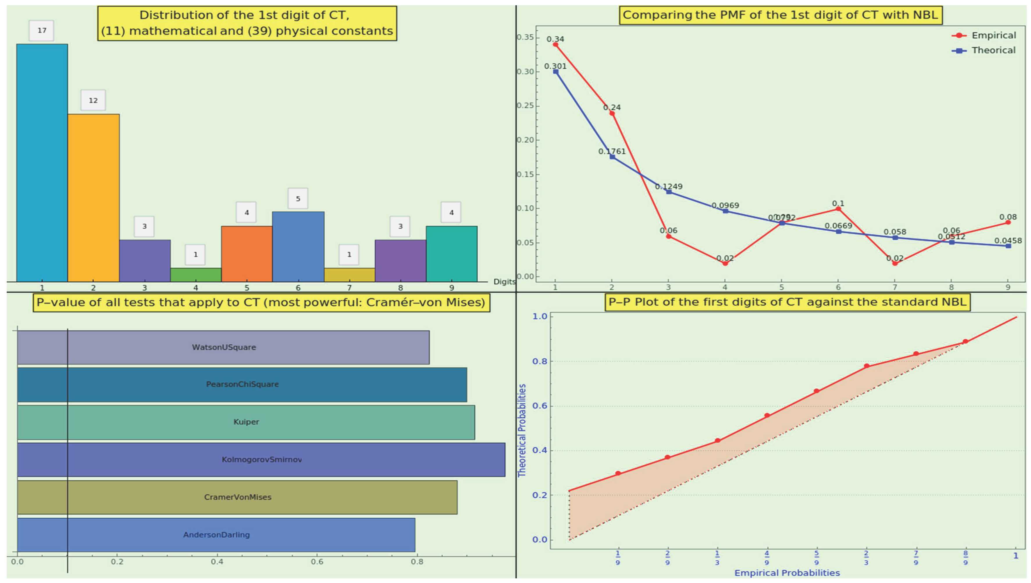
Figure 10.
We show the energy of the CT numerals and their upper limit.
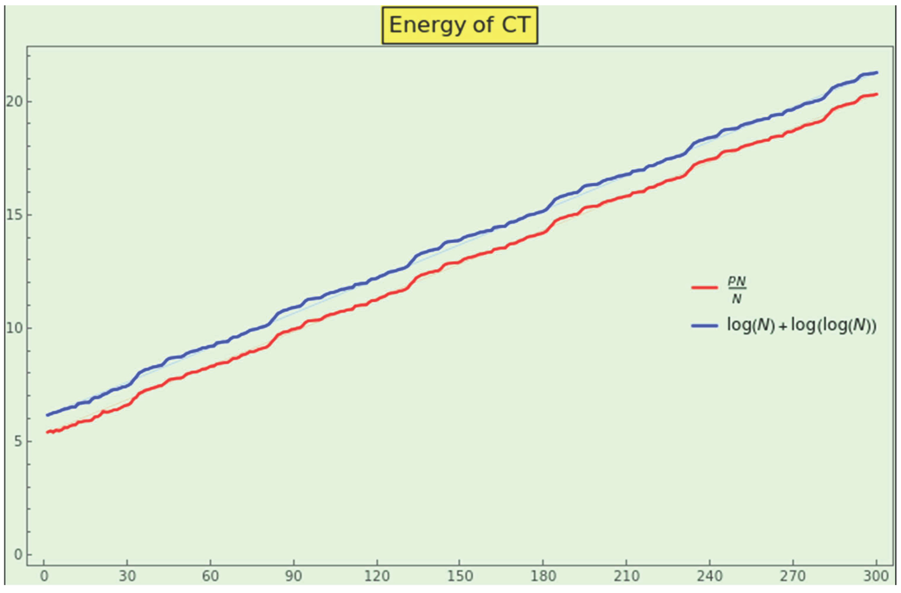
Figure 11.
Logarithmic plot of the CT ordinals (top-left) and histograms of the distribution of the SPO’s logarithm (bottom-left), prime geometric mean ordinal’s logarithm (top-right), and LPO’s logarithm (bottom-right).
Figure 11.
Logarithmic plot of the CT ordinals (top-left) and histograms of the distribution of the SPO’s logarithm (bottom-left), prime geometric mean ordinal’s logarithm (top-right), and LPO’s logarithm (bottom-right).
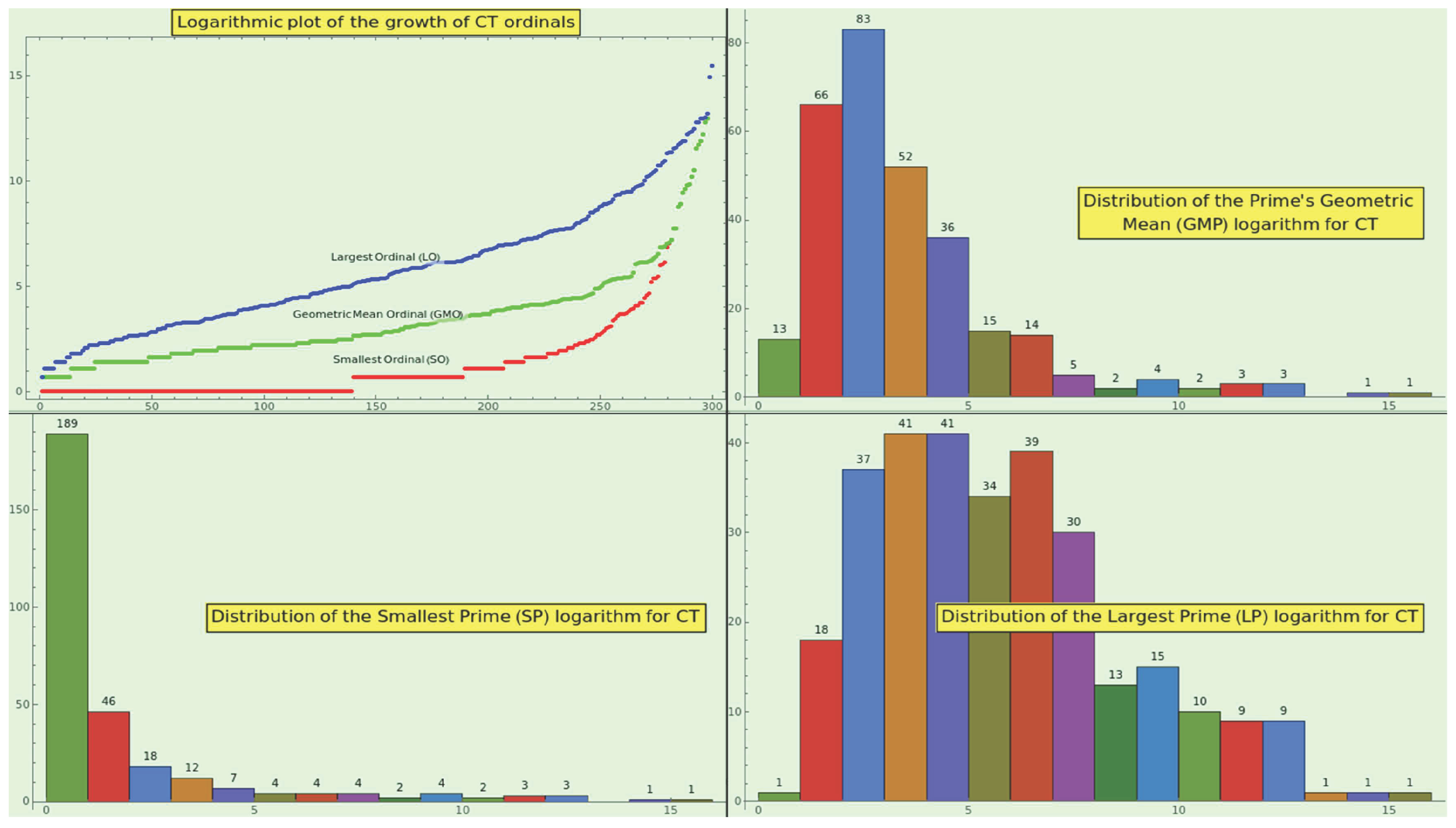
Figure 12.
Log-plot of the sums of the prime factor ordinals for every numeral in CT.
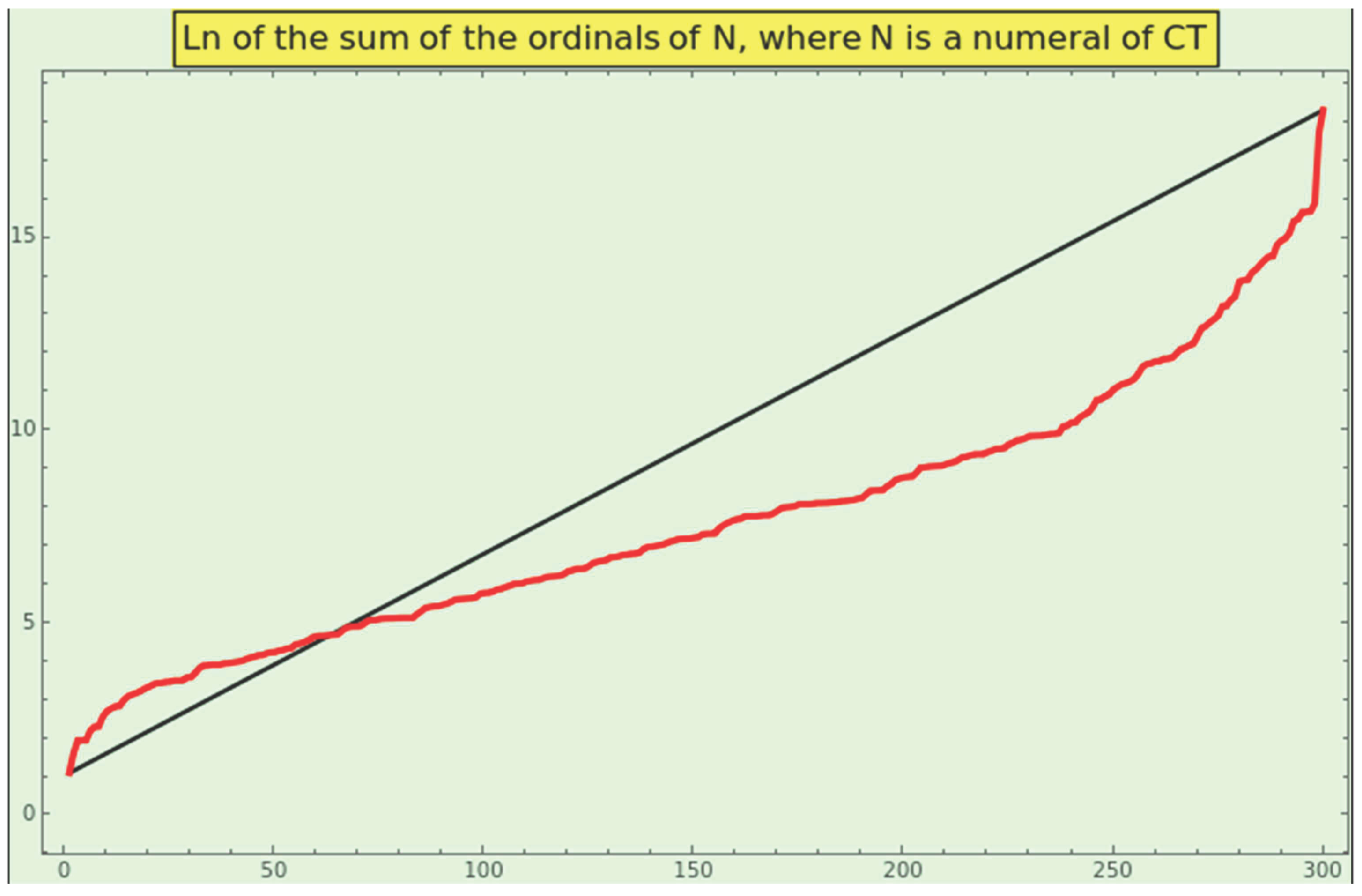
Figure 13.
Omega functions of CT.
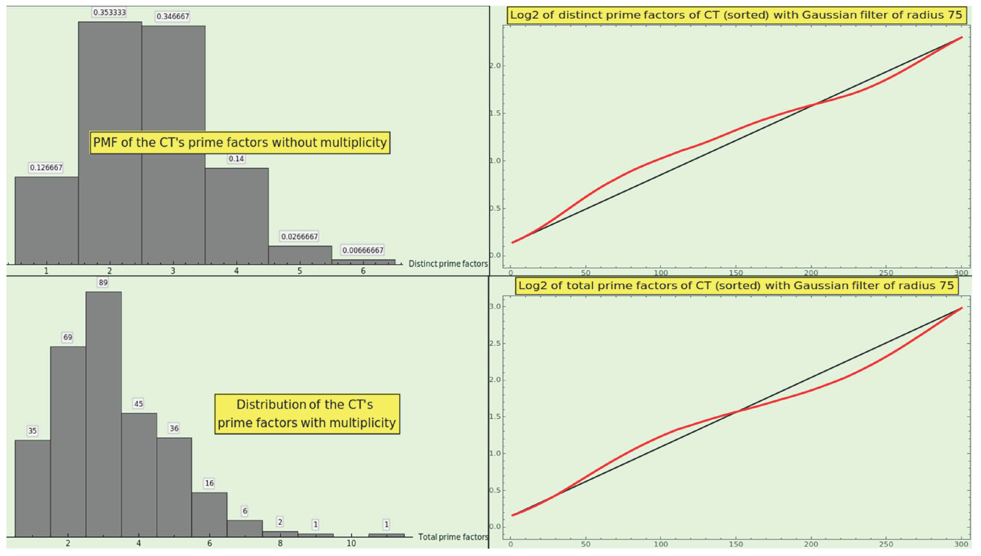
Figure 14.
Sigma functions of CT.
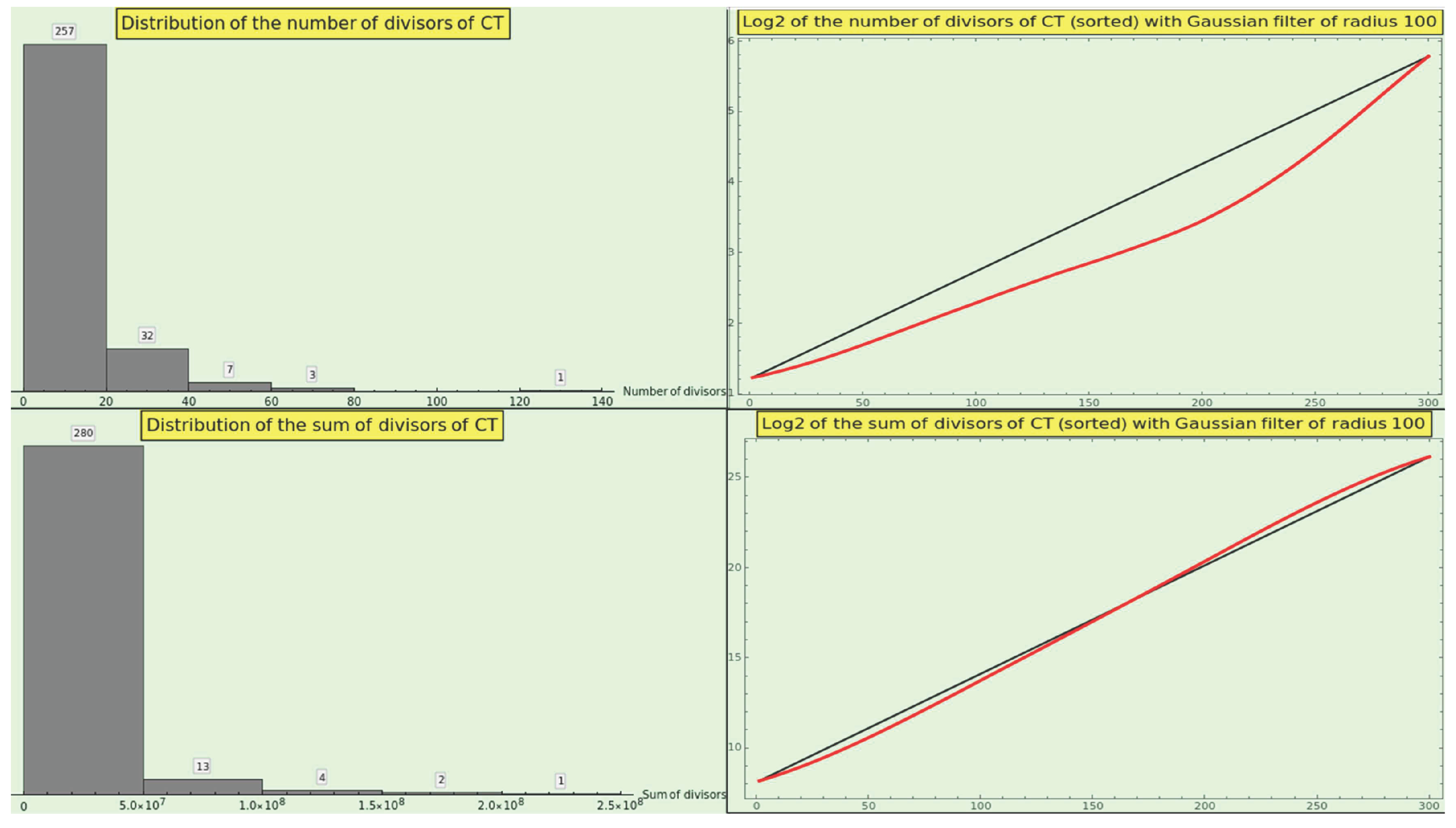
Figure 15.
Growth of the average sum of the number of divisors rendered by the CT and WP entries.
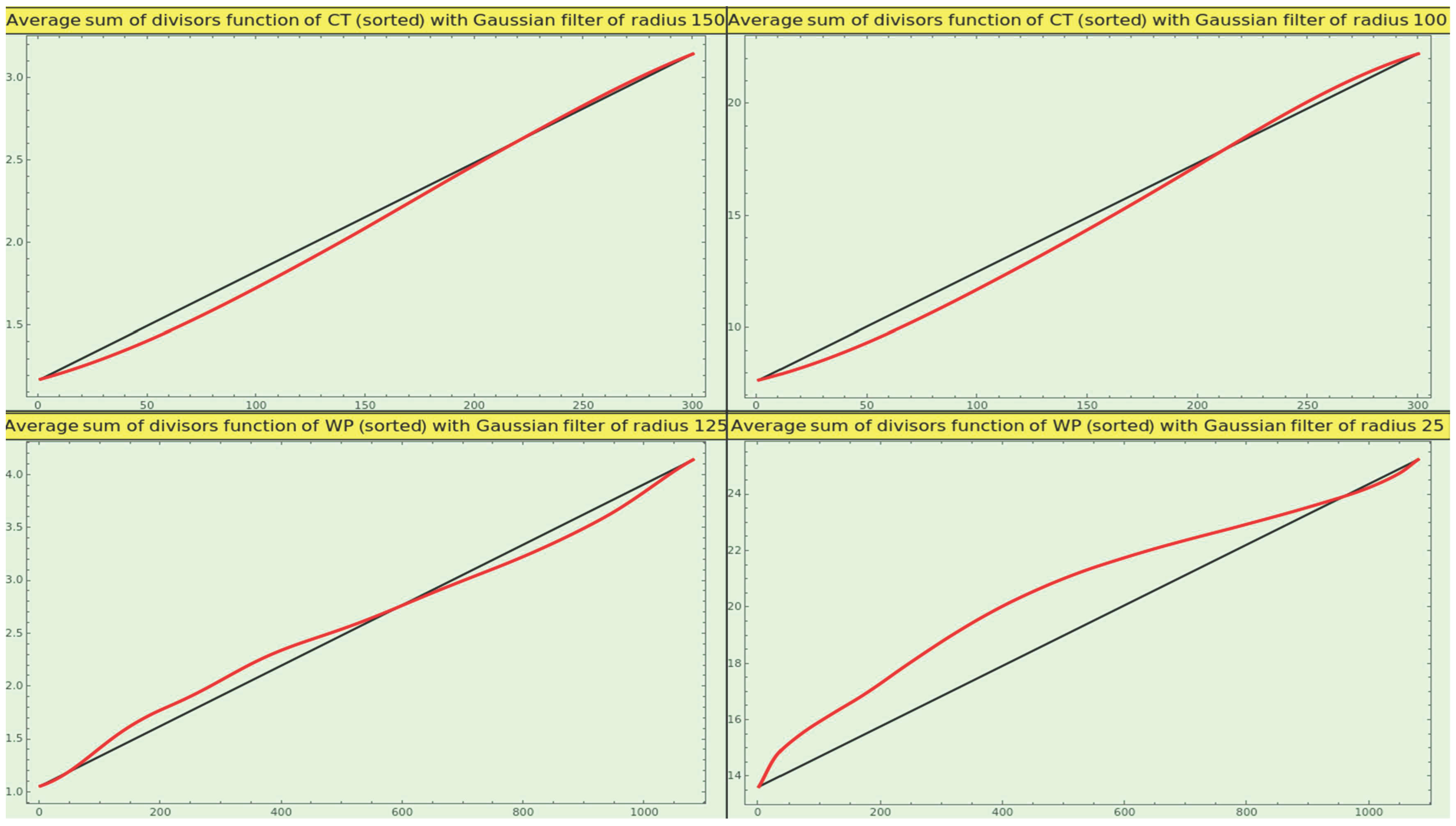
Figure 16.
Sort the numerals and calculate the natural logarithm of the highly composite counting function values to obtain the growth plot shown in the top-right corner. Now, calculate to obtain the growth plot shown in the bottom-right corner. We display the corresponding distributions on the left.
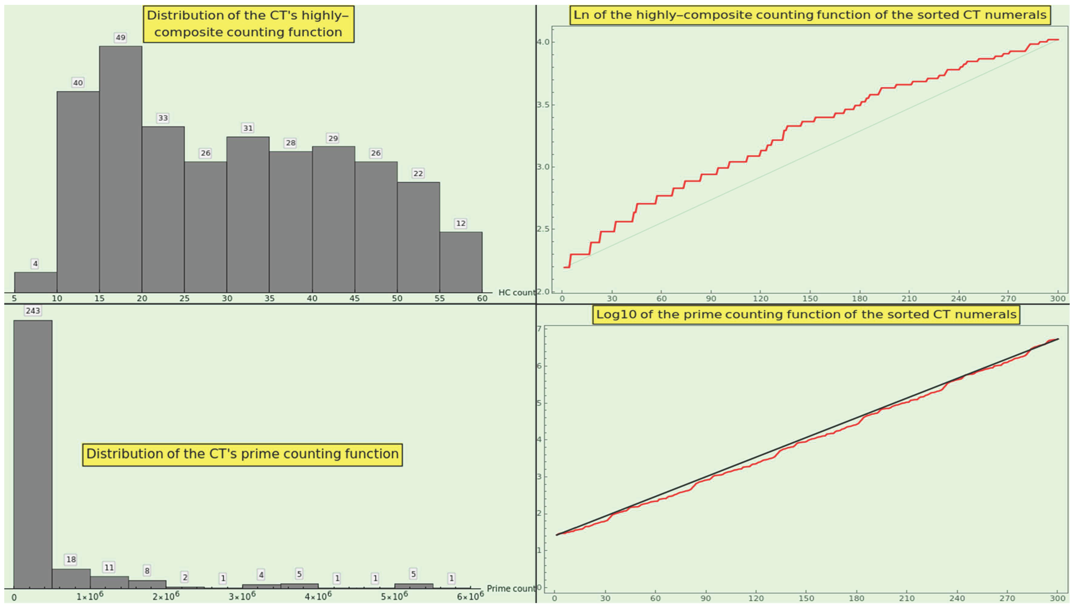
Figure 17.
Internal growth of the prime counting function of the numerals contained in CT, in red. We show the plot of the curve in black.
Figure 17.
Internal growth of the prime counting function of the numerals contained in CT, in red. We show the plot of the curve in black.
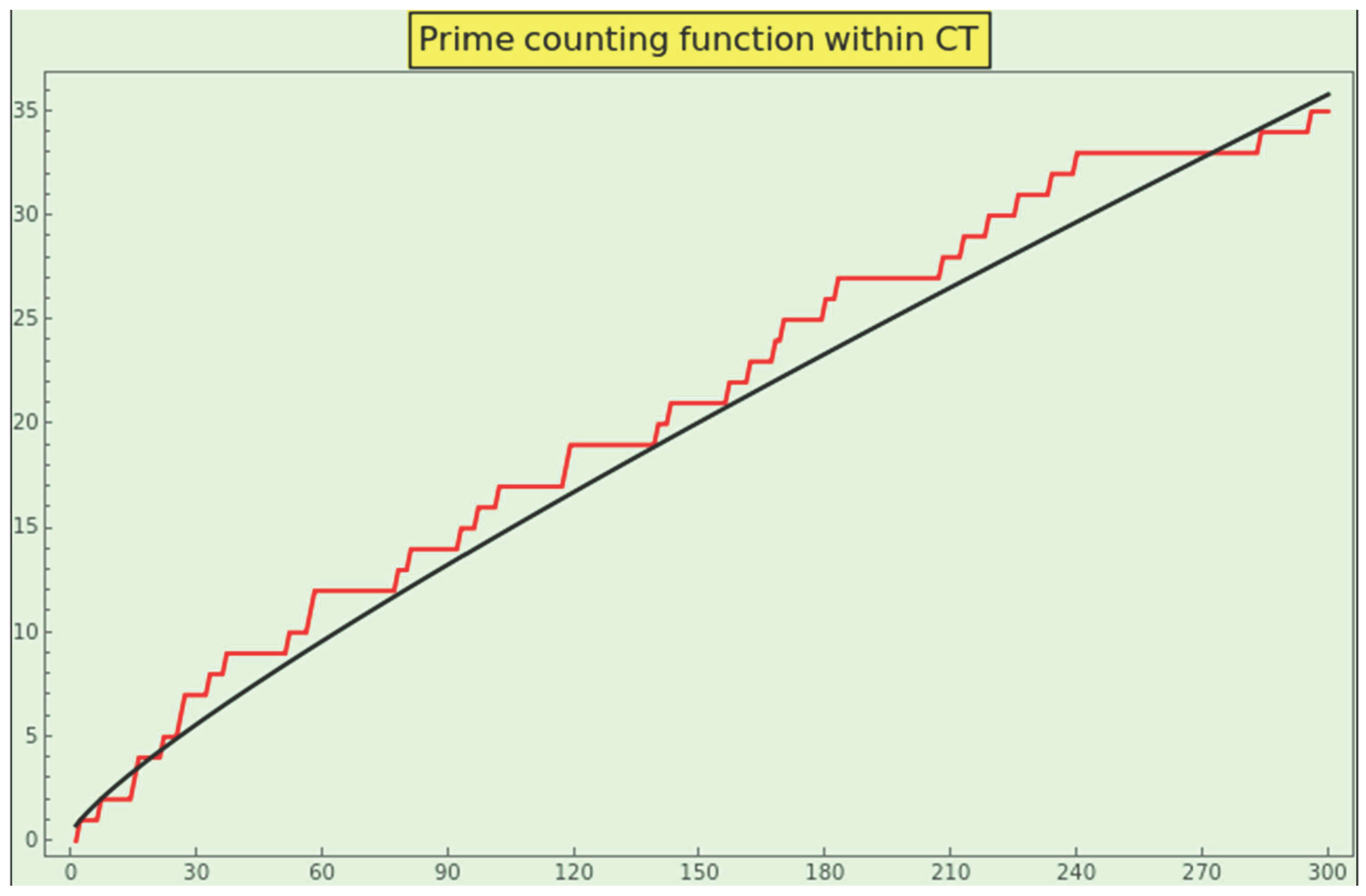
Figure 18.
Plot of all of the probability mass of the first ordinals of the factorization of CT normalized to an increasing maximal ordinal compared with the probabilistic law of the minor prime 3. We display the factorization normalized to the 96th ordinal; we cannot reject the null hypothesis that the datasets have the same distribution at the level of significance based on the Cramér-von Mises test, and even less considering that the RRMSE is below . The x-axis indicates the prime ordinal, and the y-axis indicates the occurrence frequency..
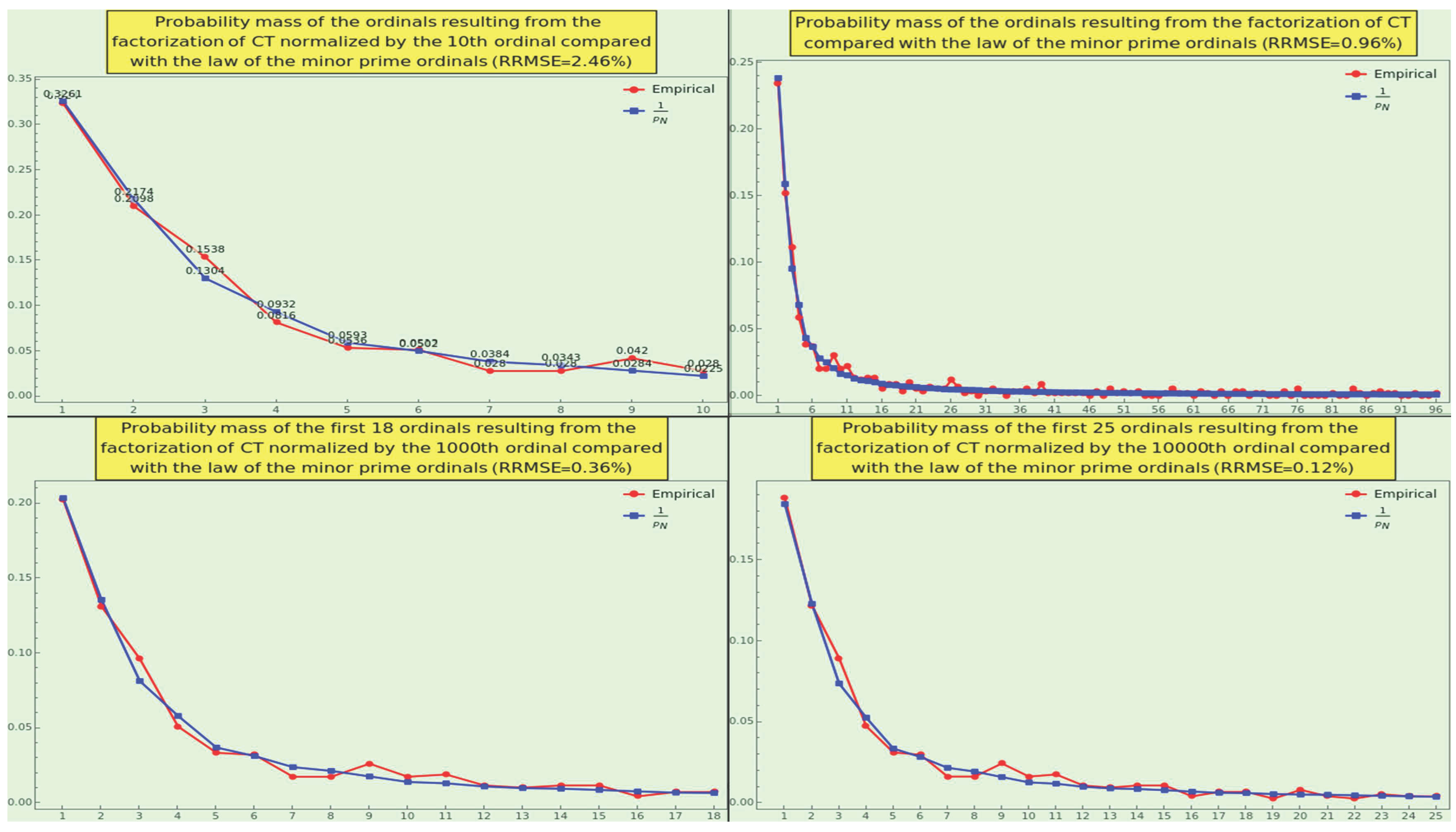
Figure 19.
Plot of the probability masses of the first SPOs of CT, normalized to an increasing maximal ordinal, compared with the probabilistic law 5. We display in full the factorization normalized to the 96th ordinal; we cannot reject the null hypothesis that the datasets have the same distribution at the level of significance based on the Cramér-von Mises test, and even less considering that the RRMSE is below . The x-axis indicates the prime ordinal N, and the y-axis indicates the occurrence frequency.
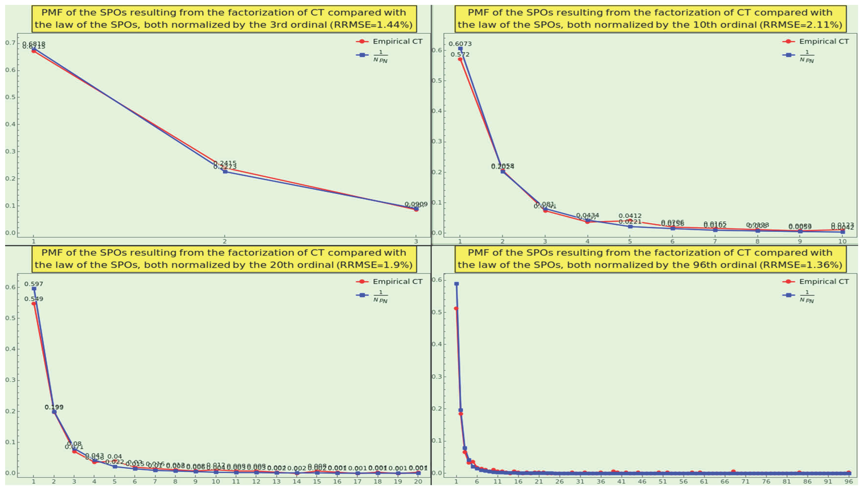
Figure 20.
The log-plot of the PMF sequences of , , , , , and are (-0.19,-0.694,-1.084,-1.432,-1.76,-2.078,-2.389,-2.697,-3.002), (-0.216,-0.649,-1.036,-1.393,-1.731,-2.057,-2.374,-2.686,-2.995), (-0.003,-2.171,-4.299,-6.405,-8.496,-10.576,-12.648,-14.714,-16.775), (-0.004,-2.017,-4.045,-6.078,-8.112,-10.148,-12.184,-14.219,-16.255), (0,-4.148,-8.198,-12.215,-16.221,-20.223,-24.224,-28.224,-32.223), and (0.,-3.959,-7.969,-11.99,-16.014,-20.037,-24.061,-28.086,-32.112), respectively. These are essentially the same curve (not a straight line), and hence constitute another sign of naturalness.
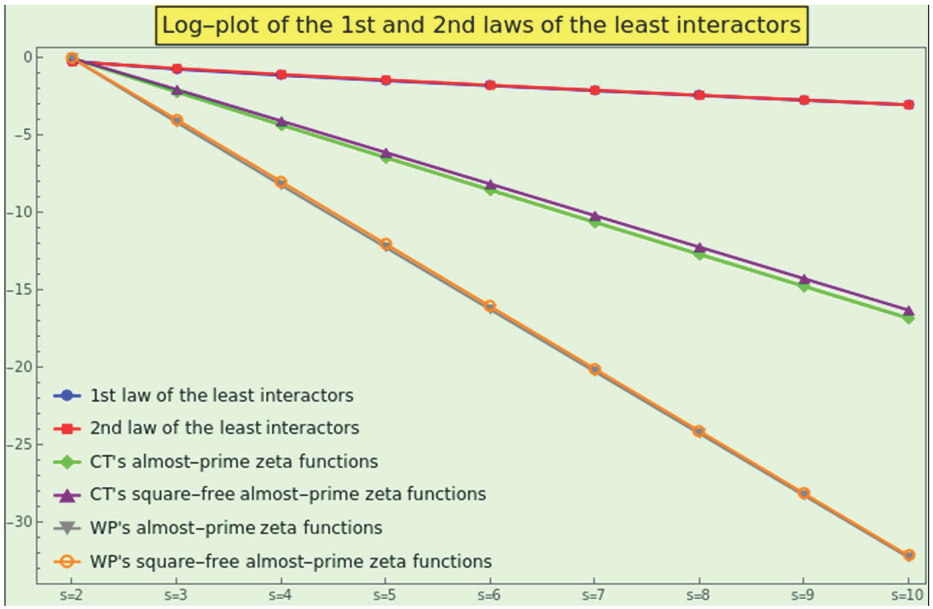
Figure 21.
At the top-left, we display the PMFs of CT, depending on k, for various values of s, after convolving the frequencies with a normal filter of radius 3. We cannot model these almost-prime profiles using a lognormal distribution; instead, we use a generalized gamma distribution. This fact explains why the log-plots for all k’s along the s-axis show a slight deviation from the straight line connecting the start (s=2) and end (s=10) points (top-right). The log-plots for all values of s along the k-axis change direction several times relative to the straight line joining the start (k=1) and end (k=9) points (bottom-left). The outline of these s-cuts is specific to CT and cannot be considered characteristic of a natural dataset. The three-dimensional log-plot in the bottom-right corner displays the complete surface of the partial sums.
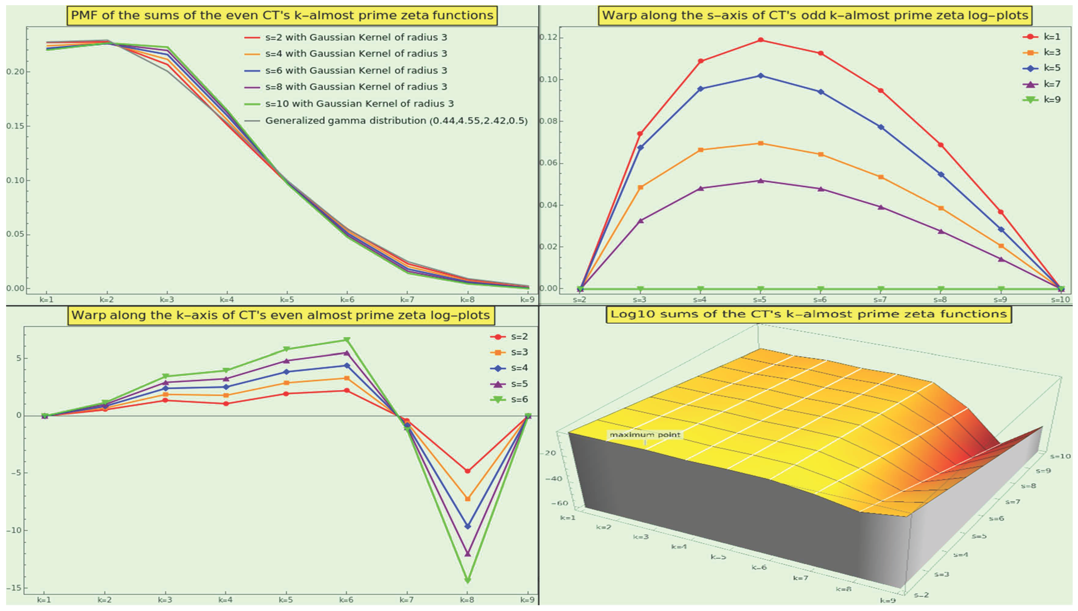
Figure 22.
At the top-left, we display the PMFs of CT, depending on k, for various values of s, after convolving the frequencies with a normal filter of radius 3. We cannot model these square-free almost-prime profiles using a lognormal distribution; instead, we use a generalized gamma distribution. This fact explains why the log-plots for all k’s along the s-axis show a slight deviation from the straight line connecting the start (s=2) and end (s=10) points (top-right). The log-plots for all values of s along the k-axis change direction several times relative to the straight line joining the start (k=1) and end (k=6) points (bottom-left). The outline of these s-cuts is specific to CT and cannot be considered characteristic of a natural dataset. The three-dimensional log-plot in the bottom-right corner displays the complete surface of the partial sums.
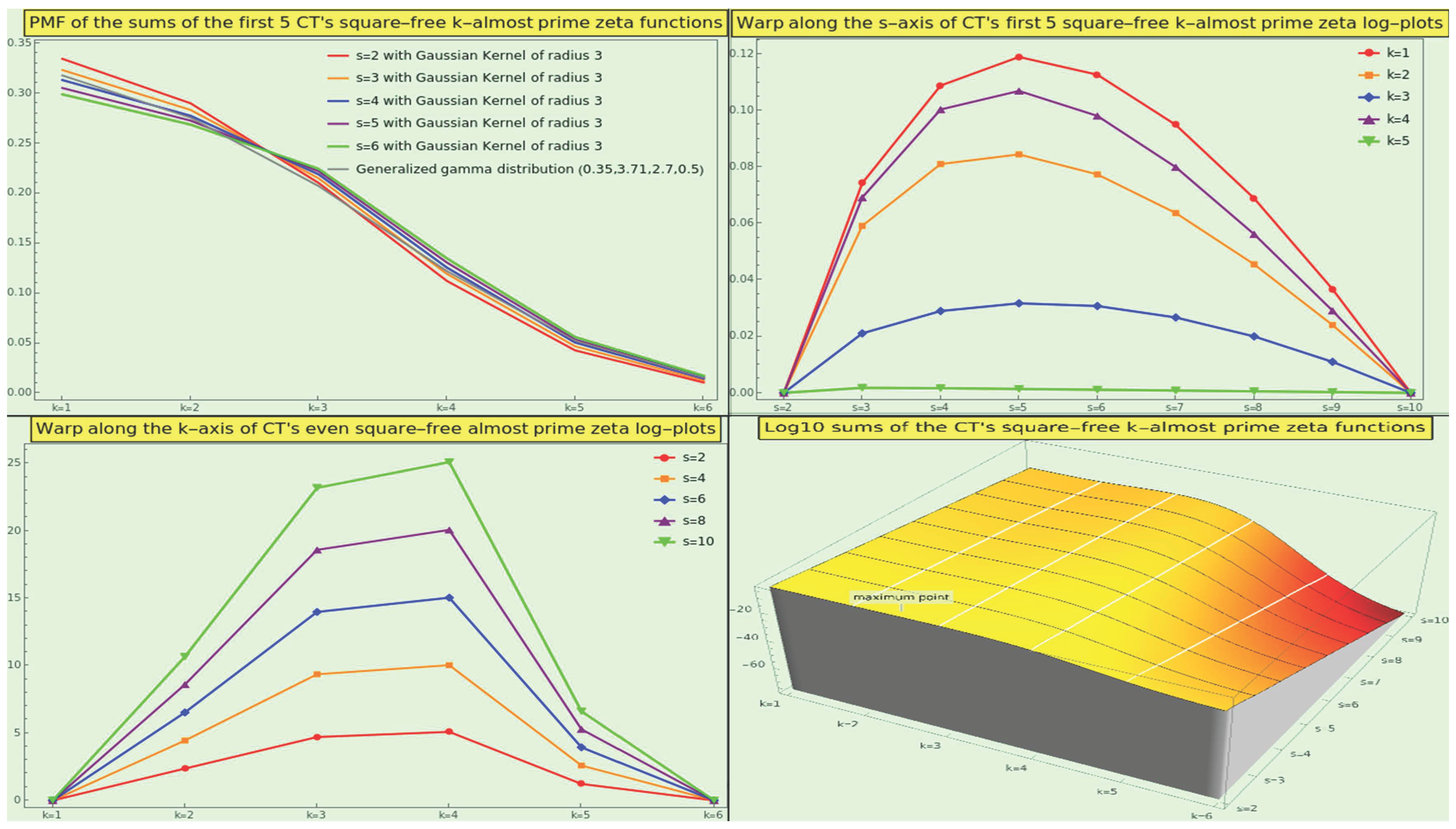
Figure 23.
Calculate for every and sort the resulting values; their plot shows linear growth of the CT totatives (top-left). Besides, we show the region of growth and plot of the intratotatives (top-right) and non-intratotatives (bottom-left), as well as the average growth of the intratotatives (bottom-right).
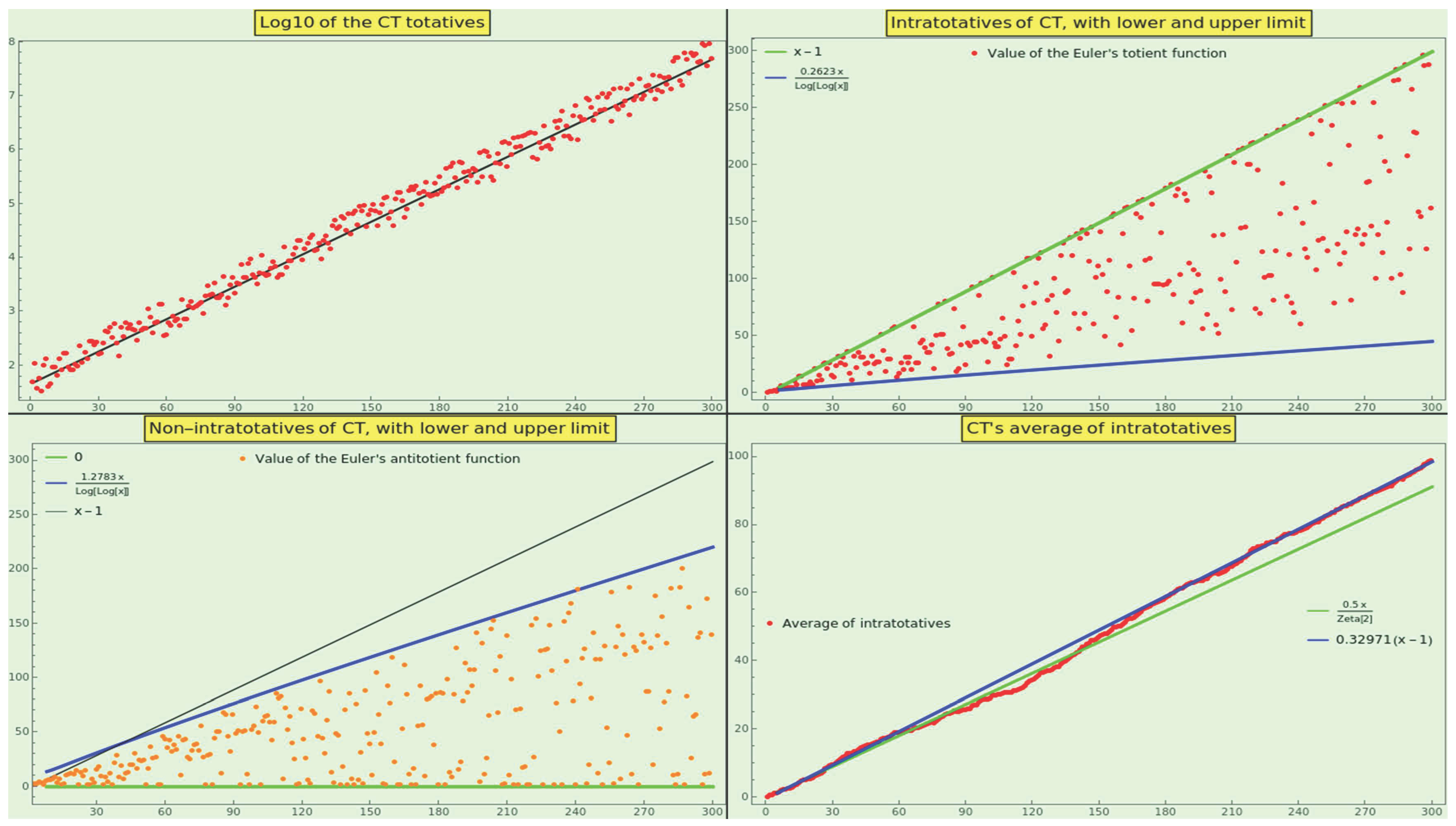
Figure 24.
The CT entries yield the histogram in the top-left corner of the figure regarding the pairwise GCD. The plot of the frequencies (empirical in red and law in blue), the p-values of the statistical test methods applied, and the P-P plot indicate that the GCD PMF of CT and the theoretical GCD PMF are hardly distinguishable.
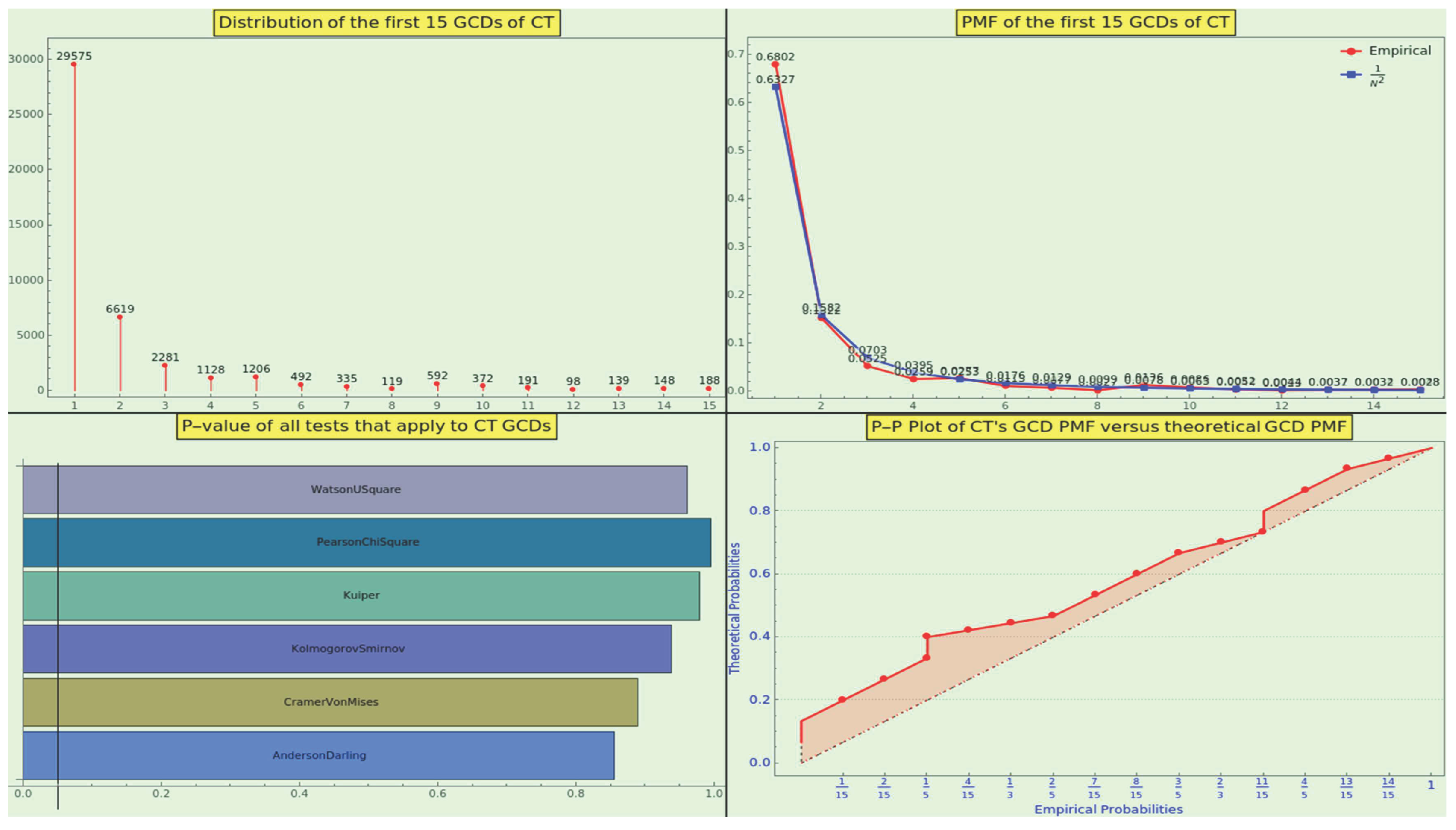
Figure 25.
Plot in red of the probability mass of the first 12 ordinals as divisors with multiplicity resulting from the factorization of CT, compared with the plot in blue of the masses resulting from the law 9. The x-axis indicates the prime ordinal o, and the y-axis indicates the occurrence frequency.
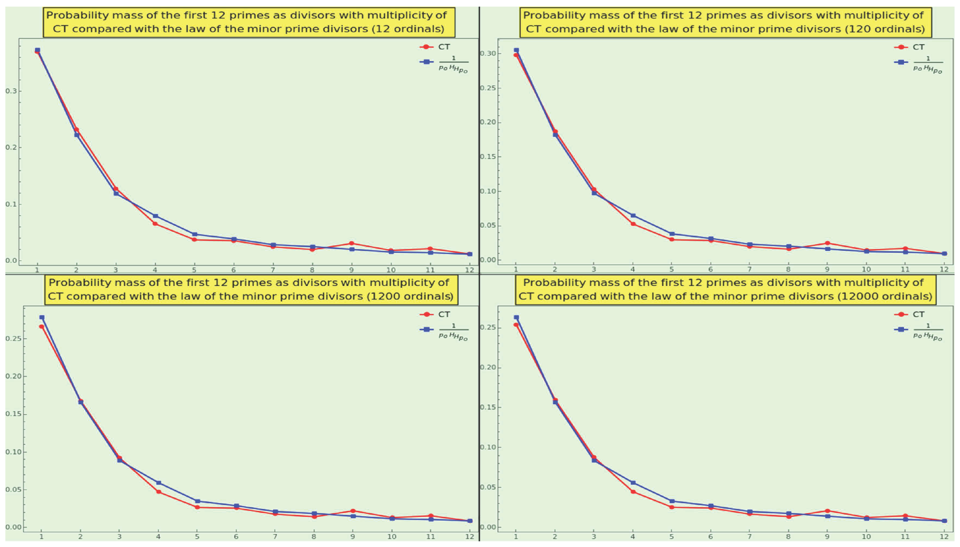
Figure 26.
Plot in red of the first 20 ordinal’s possibility masses of the prime divisors with multiplicity resulting from the factorization of CT in comparison with the theoretical frequency relative to . The x-axis indicates the prime ordinal o, and the y-axis indicates the occurrence frequency. The RRMSE between the empirical data and the data obtained from the law 10 (in blue) is excellent.
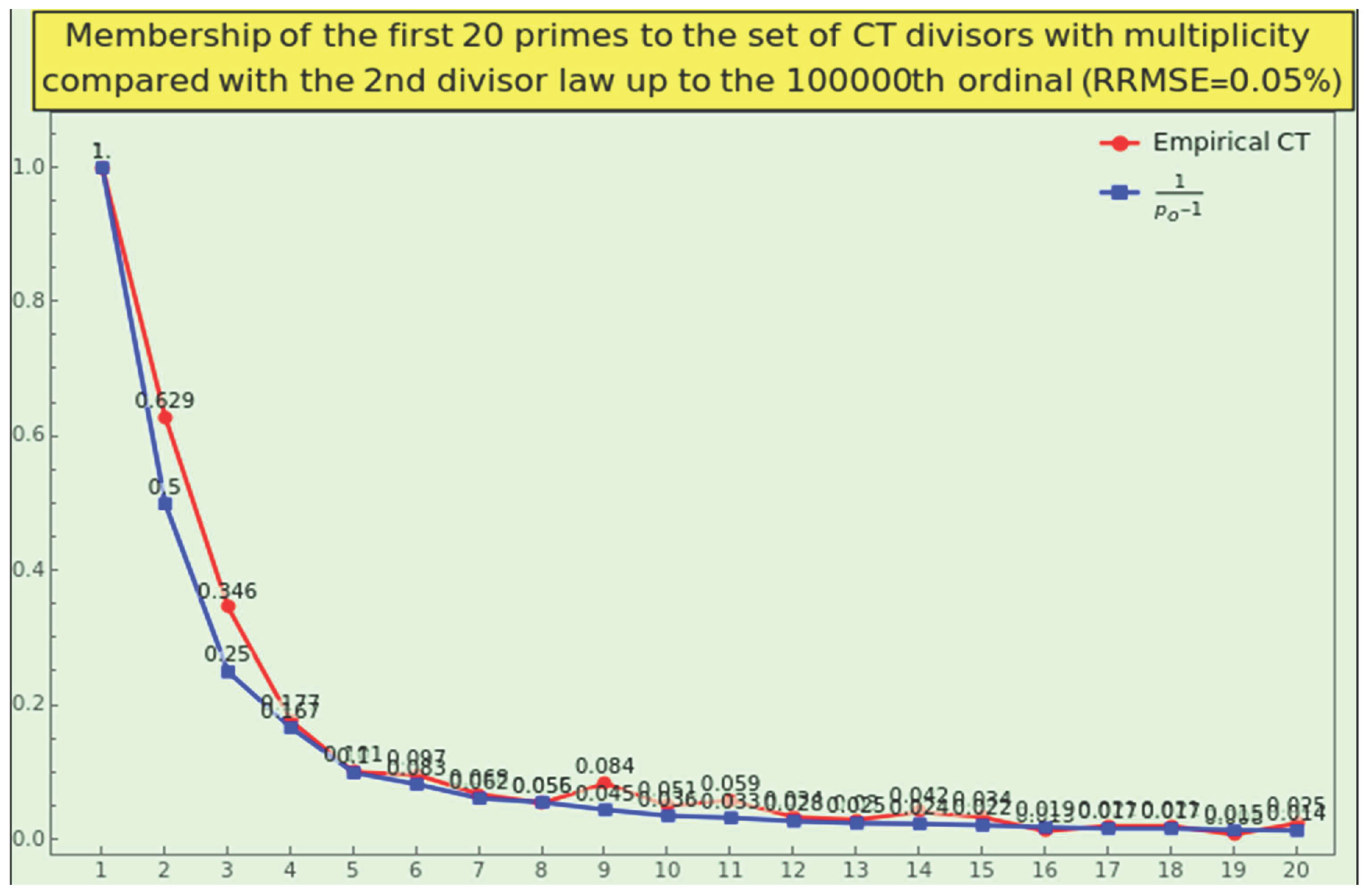
Figure 27.
The prime factorization of CT reaches the multiplicity 8, as indicated by the histogram in the top-left corner. The plot of the frequencies (empirical in red and law in blue), the p-values of the statistical test methods applied to this factorization, and the P-P plot indicate that the distributions of multiplicities are hardly distinguishable.
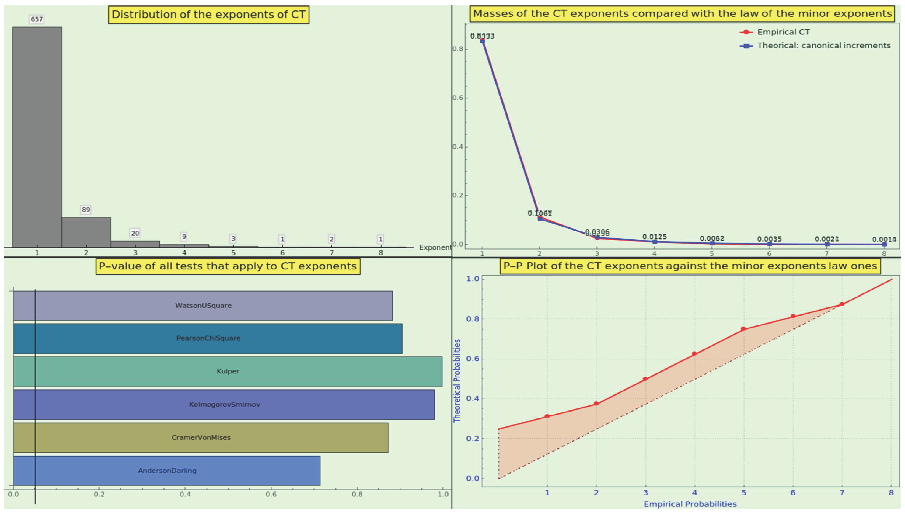
Figure 28.
The LPEs of CT reach the multiplicity 8, as indicated by the histogram in the top-left corner. The plot of the frequencies (empirical in red and law in blue), the p-values of the statistical test methods applied, and the P-P plot point to conformity.
Figure 28.
The LPEs of CT reach the multiplicity 8, as indicated by the histogram in the top-left corner. The plot of the frequencies (empirical in red and law in blue), the p-values of the statistical test methods applied, and the P-P plot point to conformity.
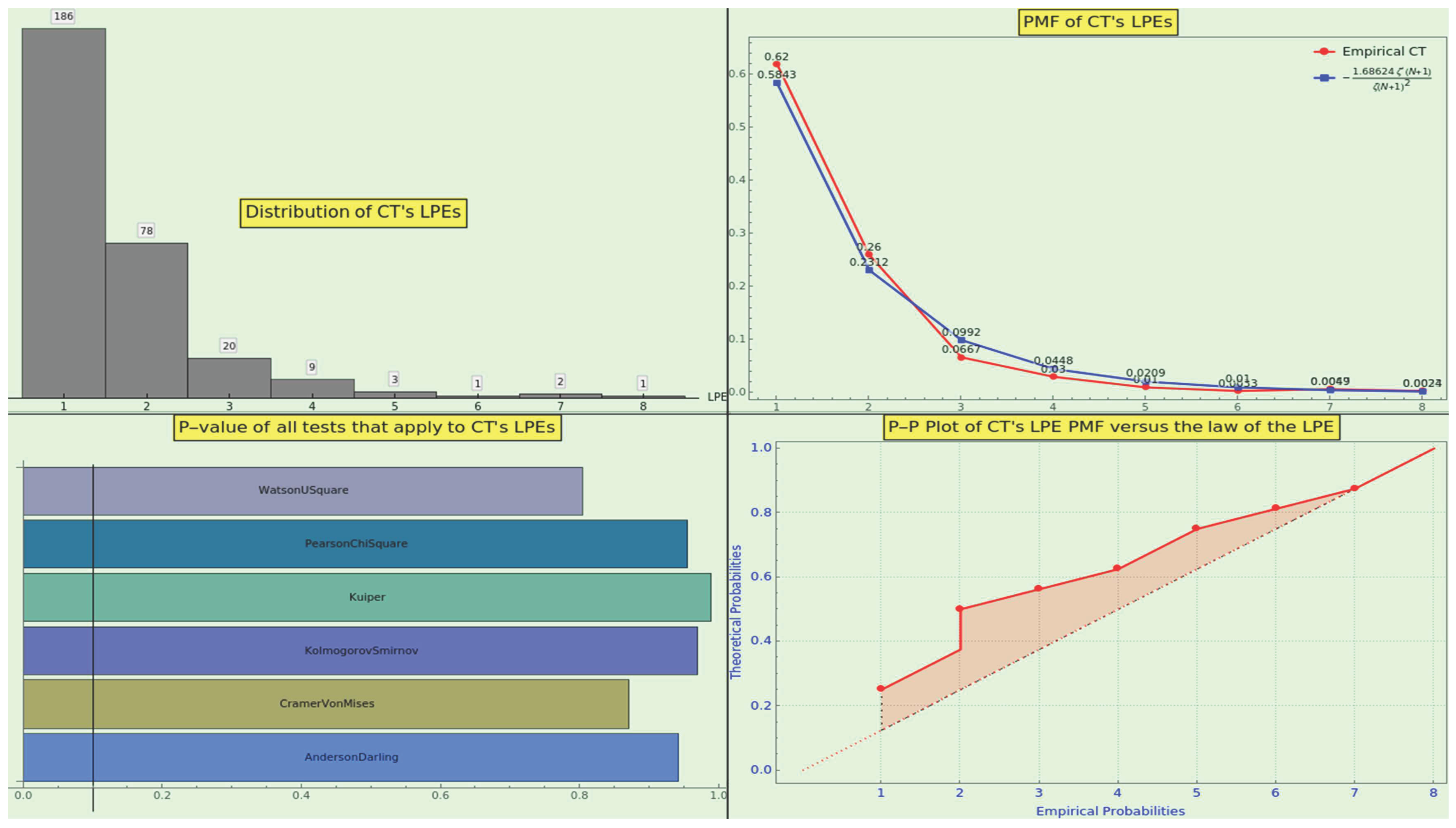
Figure 29.
WP plausibly obeys NBL.
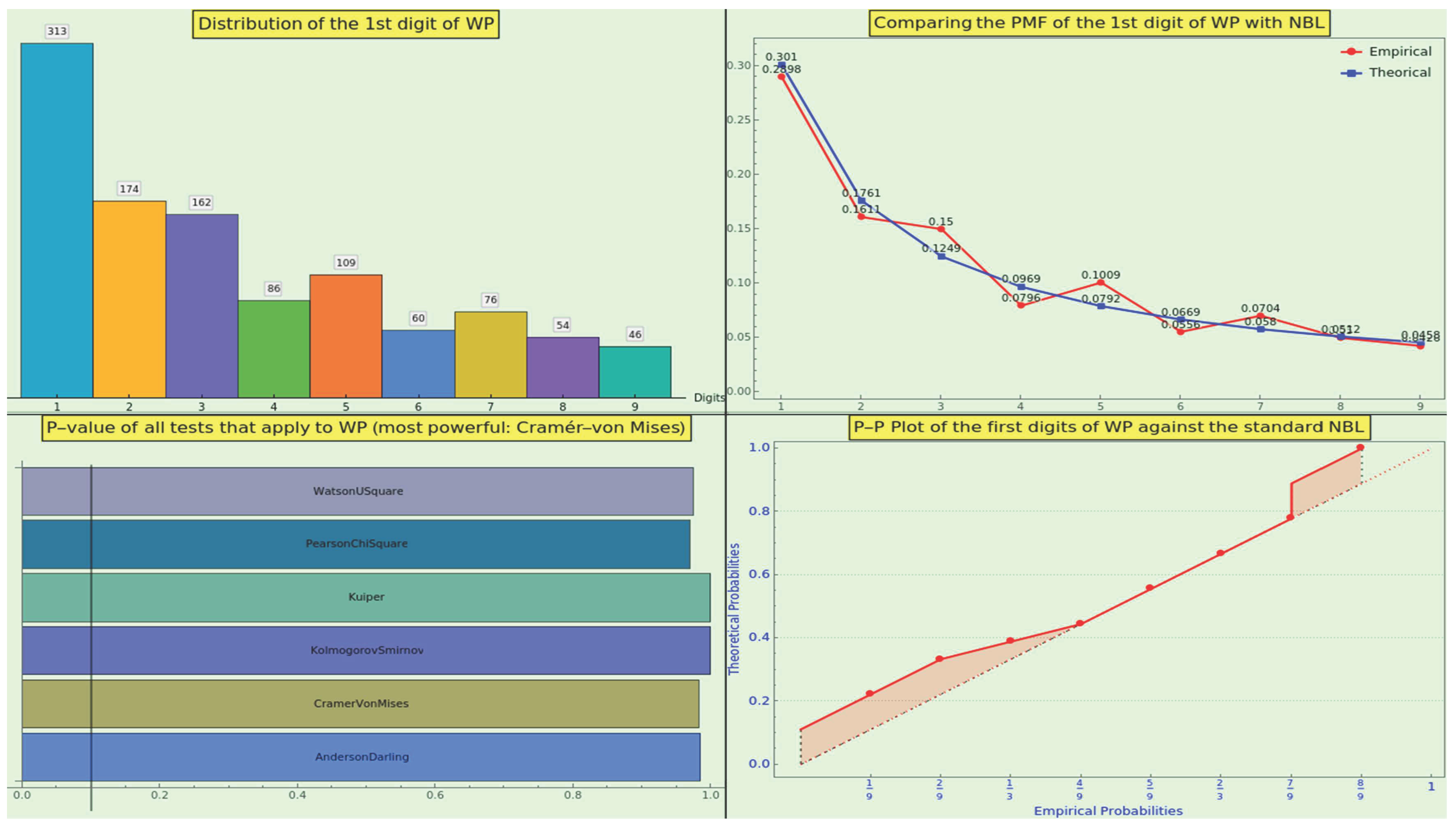
Figure 31.
Logarithmic plot of the WP ordinals (top-left) and histograms of the distribution of the SPO’s logarithm (bottom-left), prime geometric mean ordinal’s logarithm (top-right), and LPO’s logarithm (bottom-right).
Figure 31.
Logarithmic plot of the WP ordinals (top-left) and histograms of the distribution of the SPO’s logarithm (bottom-left), prime geometric mean ordinal’s logarithm (top-right), and LPO’s logarithm (bottom-right).
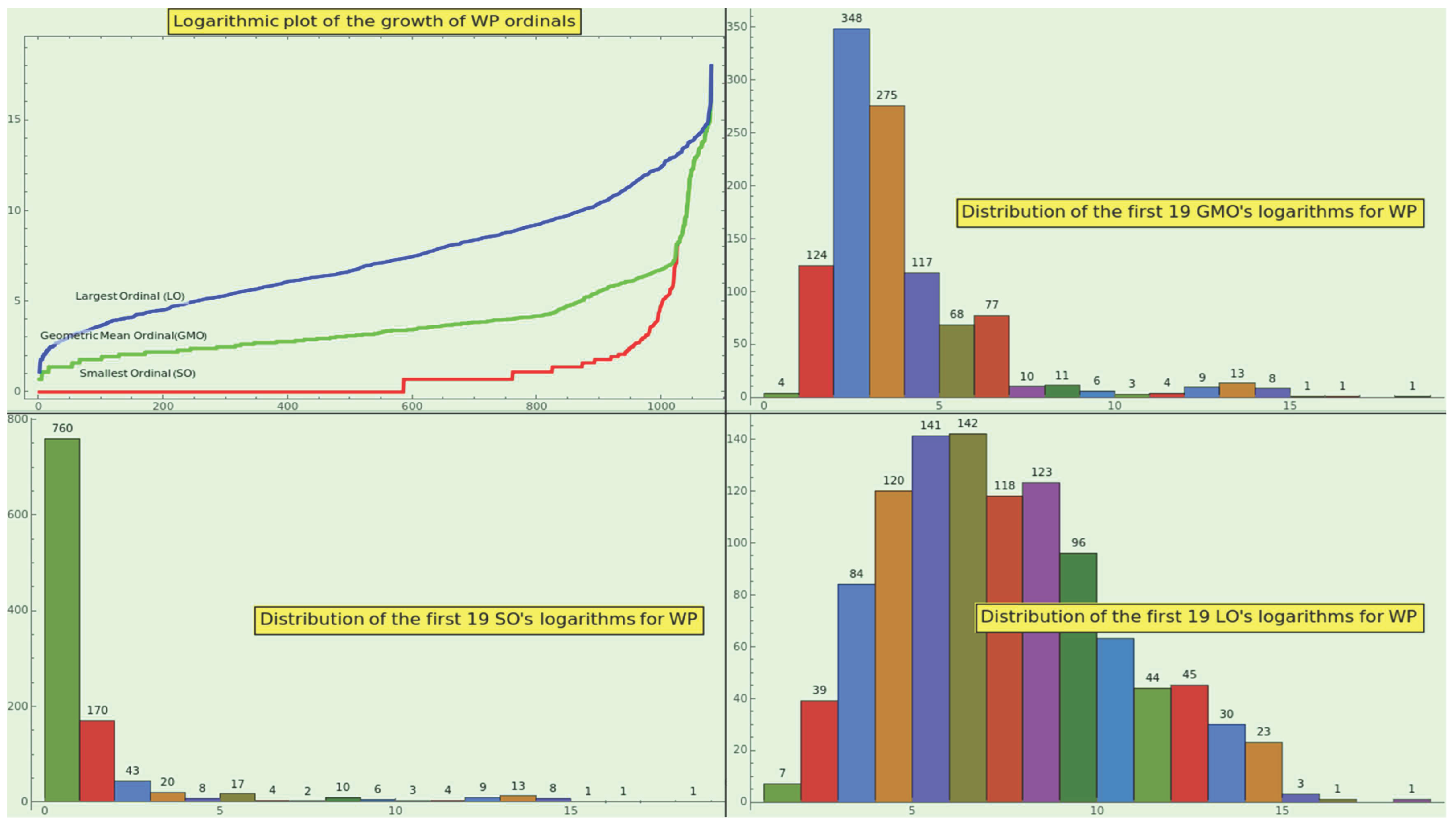
Figure 32.
Log-plot of the sums of the prime factor ordinals for every numeral in CT.
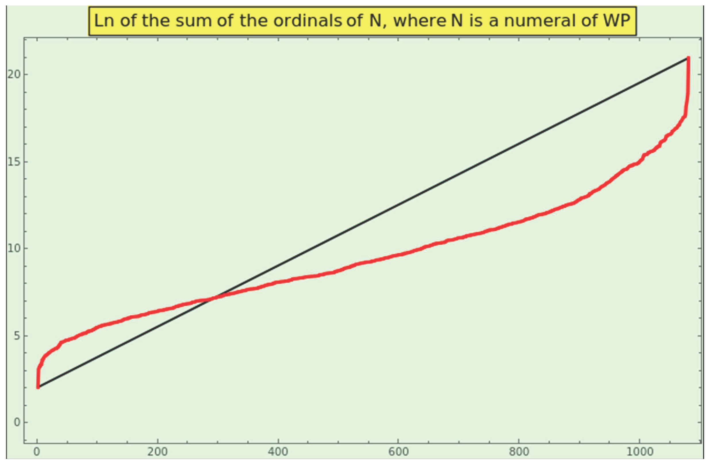
Figure 33.
Omega functions of WP.
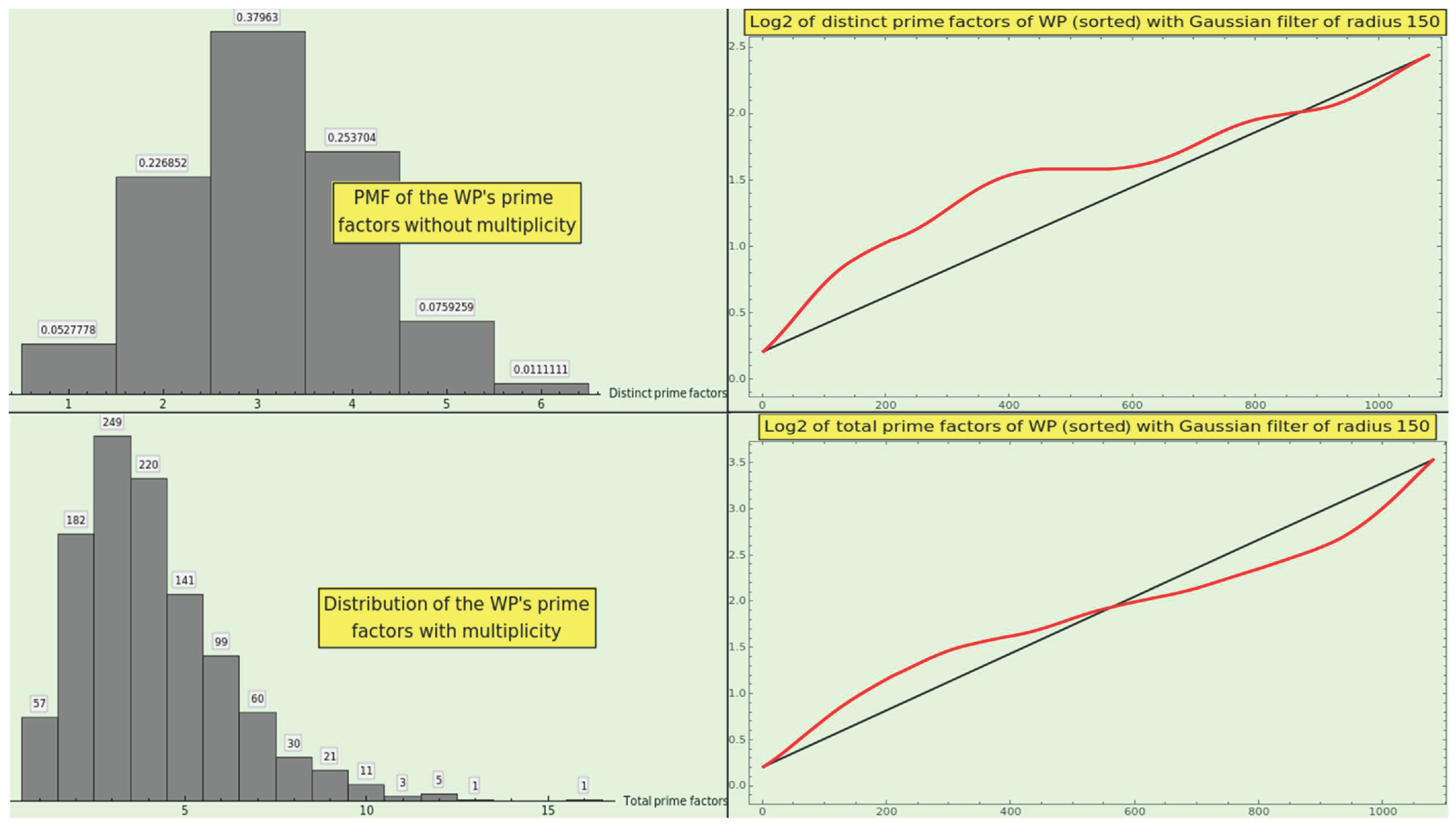
Figure 34.
Sigma functions of WP.
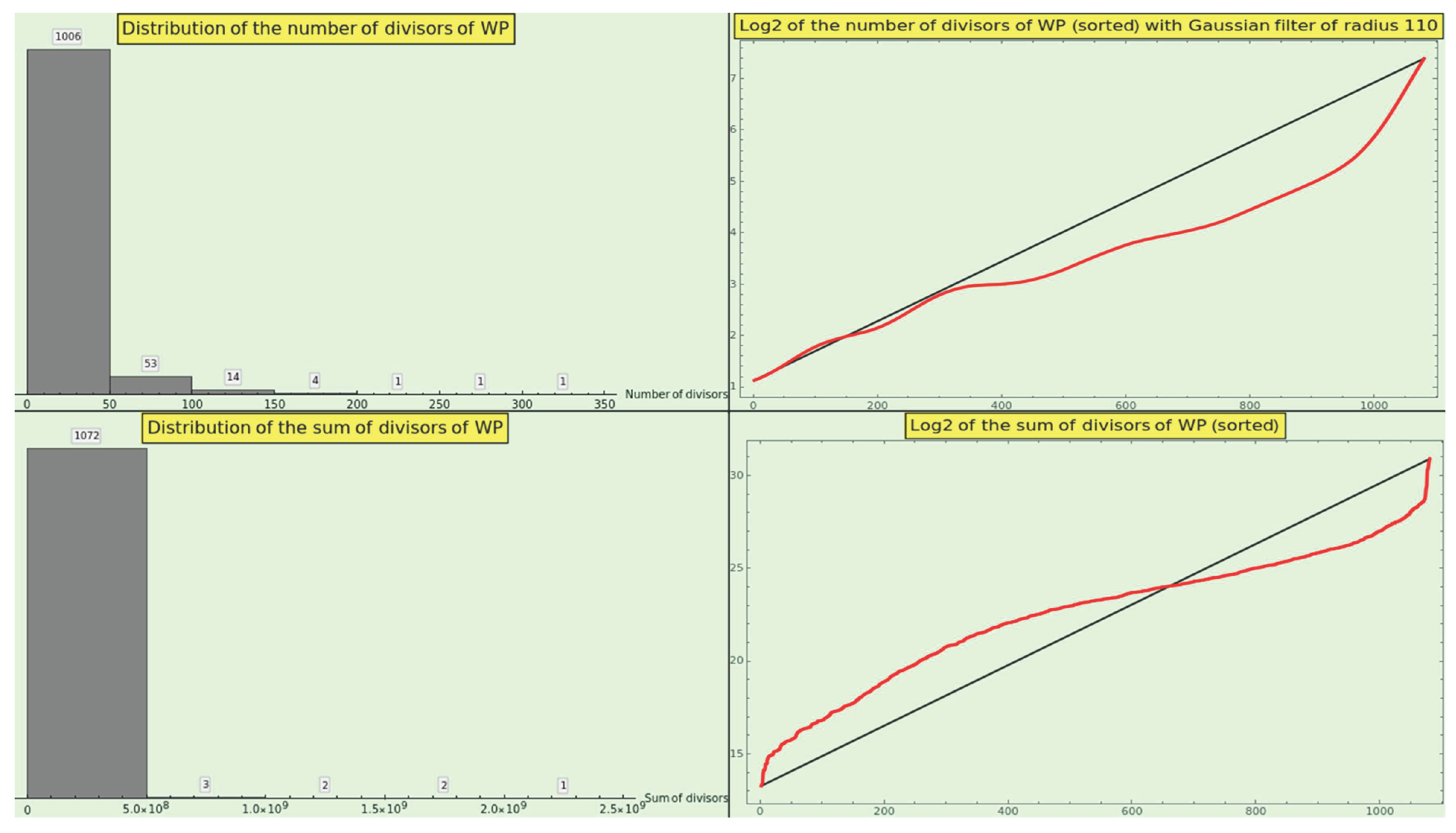
Figure 35.
Growth of the highly composite and prime numerals of WP.
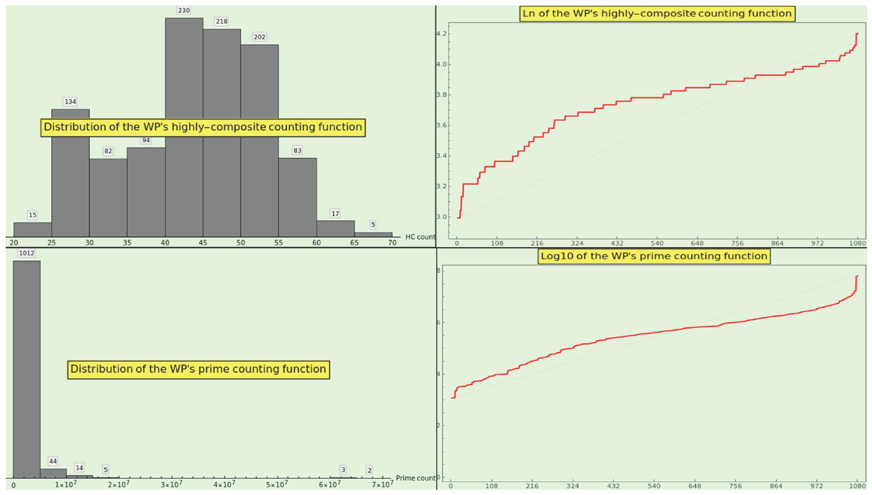
Figure 36.
Internal growth of the prime counting function of the numerals contained in WP, in red. We show the plot of the curve in black.
Figure 36.
Internal growth of the prime counting function of the numerals contained in WP, in red. We show the plot of the curve in black.
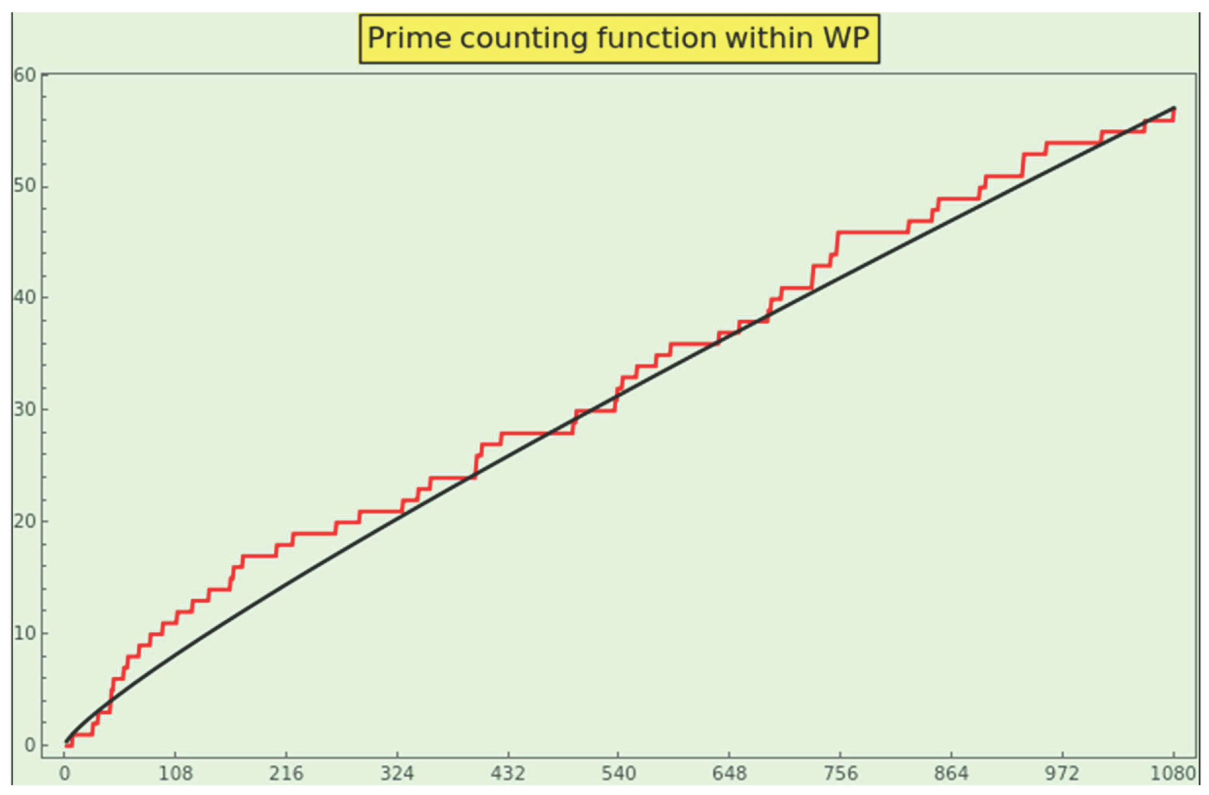
Figure 37.
Plot of the probability masses of the first WP primes, normalized to an increasing maximal ordinal, compared with the probabilistic law of the minor prime ordinals 3. We display in full the factorization normalized to the 96th ordinal; we cannot reject the null hypothesis that the datasets have the same distribution at the based on the Anderson-Darling test, with RRMSE . The x-axis indicates the prime ordinal N, and the y-axis indicates the occurrence frequency.
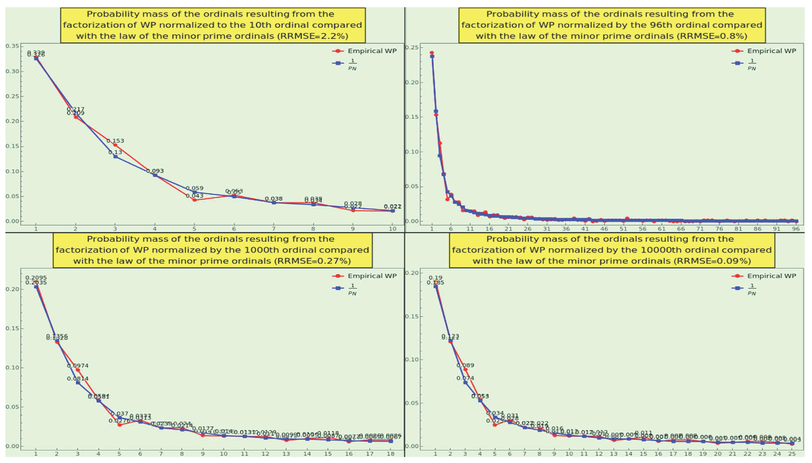
Figure 38.
Plot of the probability masses of the first SPOs of WP, normalized to an increasing maximal ordinal, compared with the probabilistic law of the minor prime 5. We display in full the factorization normalized to the 96th ordinal; we cannot reject the null hypothesis that the datasets have the same distribution at the level of significance based on the Cramér-von Mises test, and even less considering that the RRMSE is below . The x-axis indicates the prime ordinal N, and the y-axis indicates the occurrence frequency.
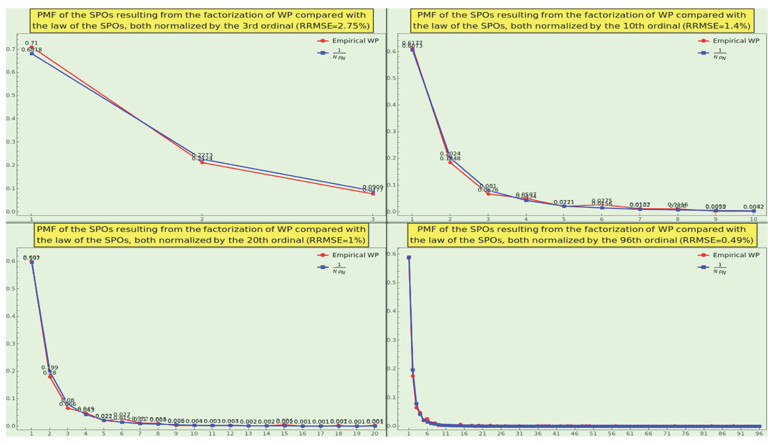
Figure 39.
At the top-left, we display, depending on k, the square-free almost-prime zeta function PMFs of the WP elements for various values of s, after calculating the convolution of the frequencies with a normal filter of radius 3. We cannot model these almost-prime profiles using a lognormal distribution; instead, we use a generalized gamma distribution. This fact explains why the log-plots for all k’s along the s-axis show a slight deviation from the straight line connecting the start (s=2) and end (s=10) points (top-right). The log-plots for all values of s along the k-axis change direction several times and even cross the straight line joining the start (k=1) and end (k=13) points (bottom-left). The outline of these s-cuts is specific to WP and cannot be considered characteristic of a natural dataset. The three-dimensional log-plot in the bottom-right corner displays the complete surface of the square-free partial sums.

Figure 40.
At the top-left, we display the square-free almost-prime zeta function PMFs of the WP elements, depending on k, for various values of s, after calculating the convolution of the frequencies with a normal filter of radius 3. We cannot model these square-free almost-prime profiles using a lognormal distribution; instead, we use a generalized gamma distribution. This fact explains why the log-plots for all k’s along the s-axis show a slight deviation from the straight line connecting the start (s=2) and end (s=10) points (top-right). The log-plots for all values of s along the k-axis change direction several times relative to the straight line joining the start (k=1) and end (k=6) points (bottom-left). The outline of these s-cuts is specific to WP and cannot be considered characteristic of a natural dataset. The three-dimensional log-plot in the bottom-right corner displays the complete surface of the partial sums.
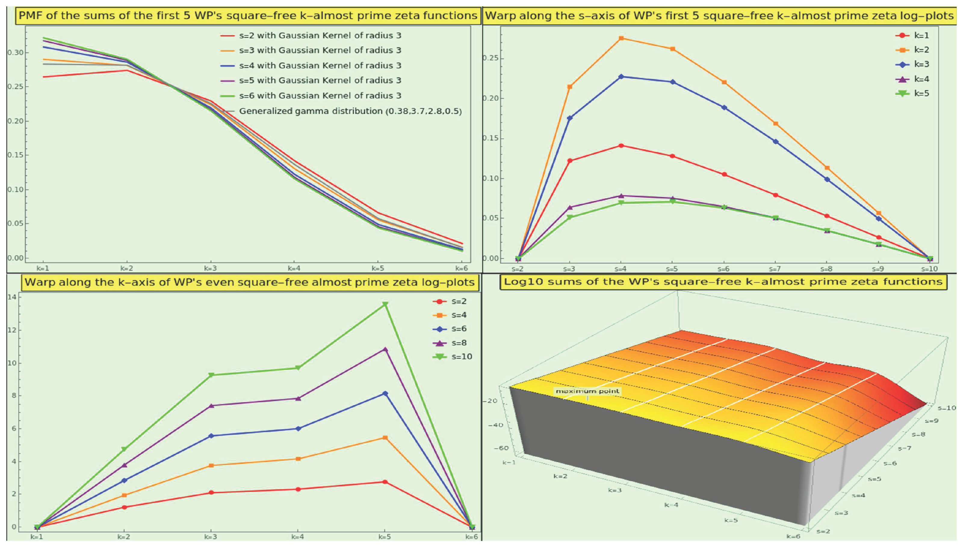
Figure 41.
Growth of the WP totatives (top-left), region of growth and plot of the intratotatives (top-right) and non-intratotatives (bottom-left), and average growth of the intratotatives (bottom-right).
Figure 41.
Growth of the WP totatives (top-left), region of growth and plot of the intratotatives (top-right) and non-intratotatives (bottom-left), and average growth of the intratotatives (bottom-right).
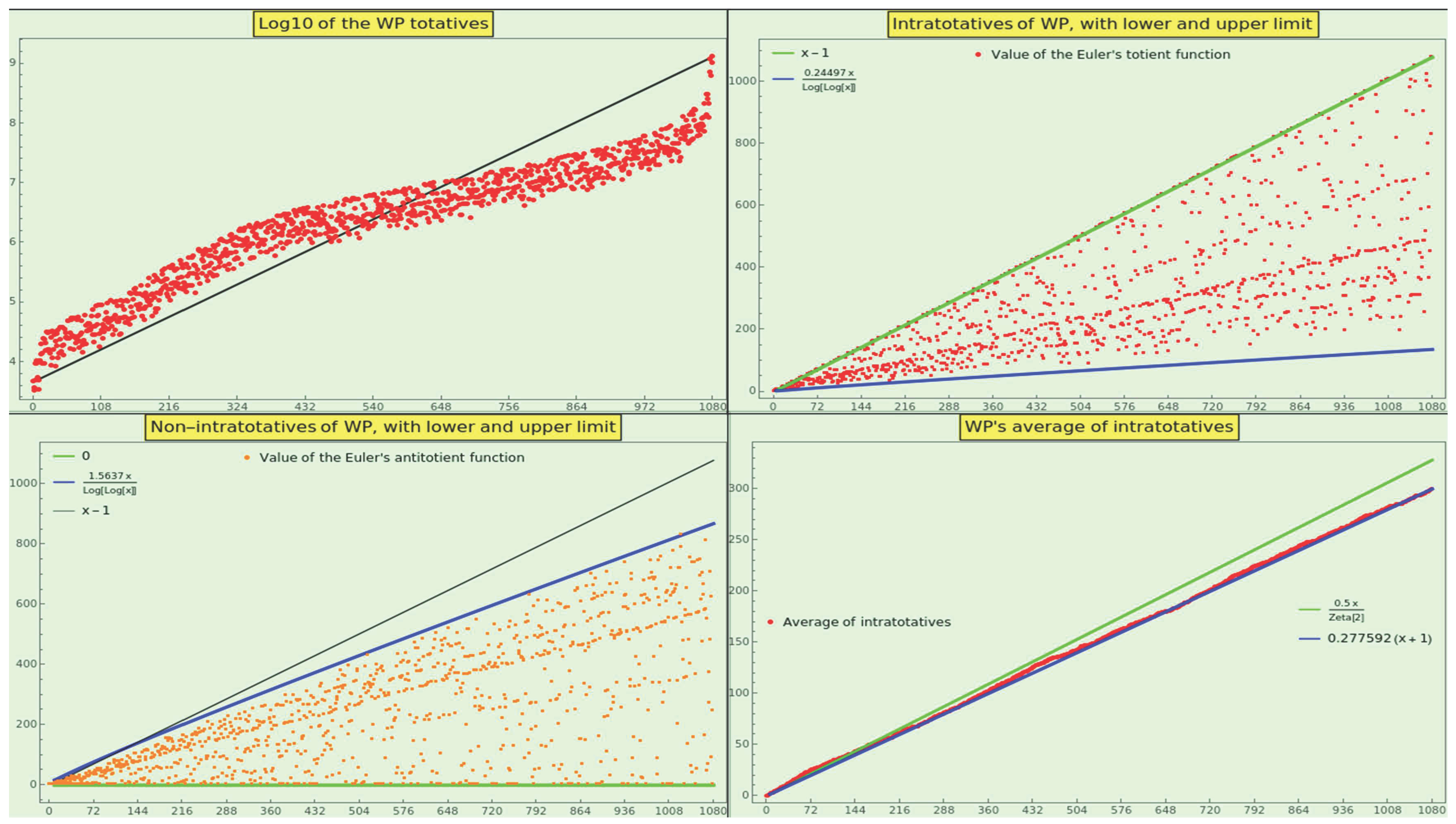
Figure 42.
The WP entries yield the histogram in the top-left corner. The plot of the frequencies (empirical in red and law in blue), the p-values of the statistical test methods applied, and the P-P plot indicate that the GCD PMF of WP and the theoretical GCD PMF are hardly distinguishable.
Figure 42.
The WP entries yield the histogram in the top-left corner. The plot of the frequencies (empirical in red and law in blue), the p-values of the statistical test methods applied, and the P-P plot indicate that the GCD PMF of WP and the theoretical GCD PMF are hardly distinguishable.
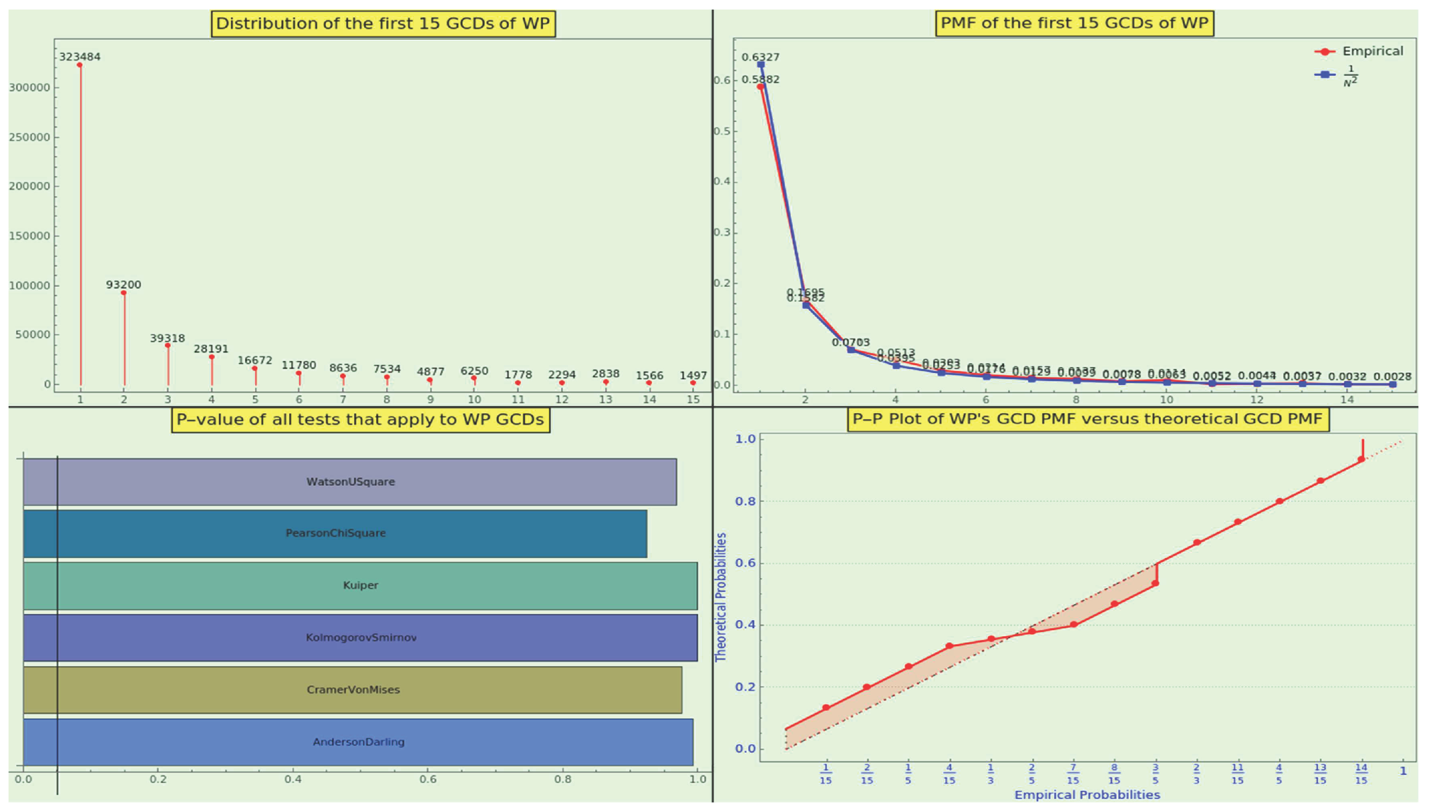
Figure 43.
Plot in red of the probability mass of the first 12 ordinals as divisors with multiplicity resulting from the factorization of WP, compared with the plot in blue of the masses resulting from law 9. The x-axis indicates the prime ordinal o, and the y-axis indicates the occurrence frequency.
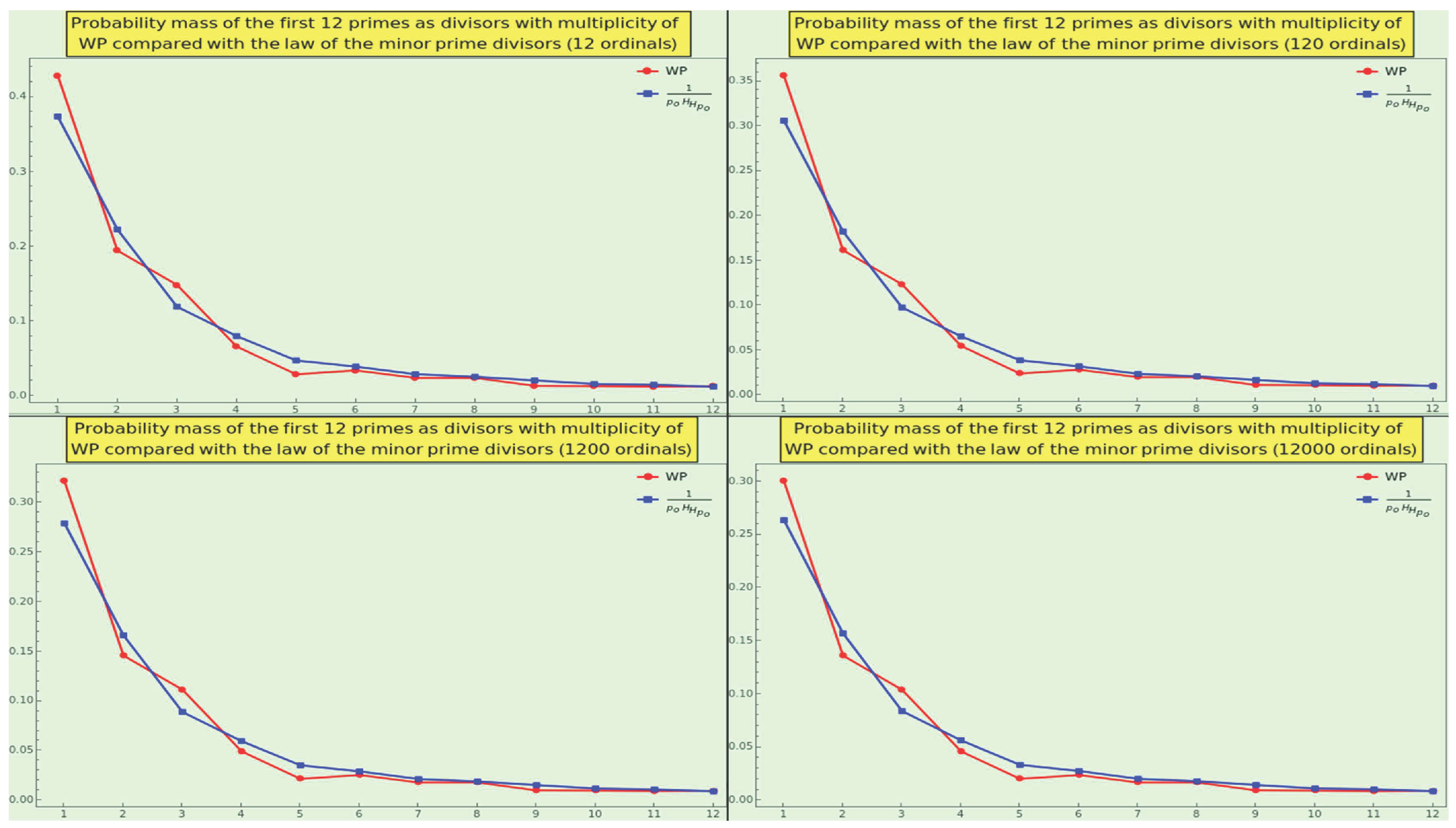
Figure 44.
Plot in red of the first 20 ordinal’s possibility masses of the prime divisors with multiplicity resulting from the factorization of WP in comparison with the theoretical frequency relative to . The x-axis indicates the prime ordinal o, and the y-axis indicates the occurrence frequency. The RRMSE between the empirical data and the data obtained from the law 10 (in blue) is excellent.
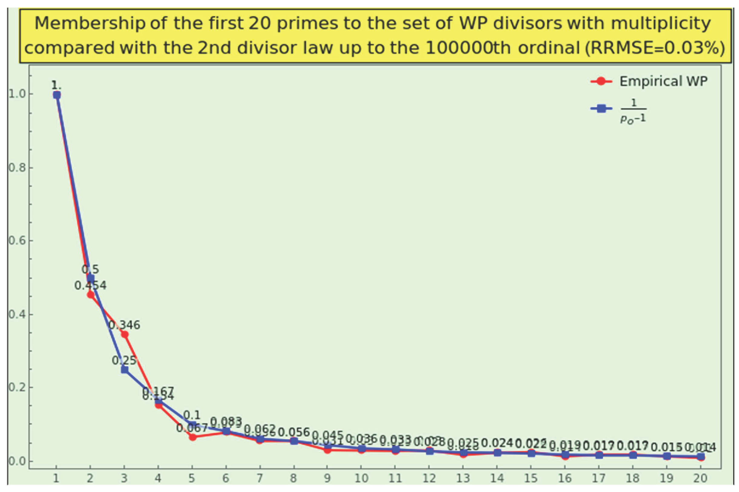
Figure 45.
The prime factorization of WP reaches the multiplicity 11, as indicated by the histogram in the top-left corner. The plot of the frequencies (empirical in red and law in blue), the p-values of the statistical test methods applied to this factorization, and the P-P plot indicate that the distributions of multiplicities are hardly distinguishable.
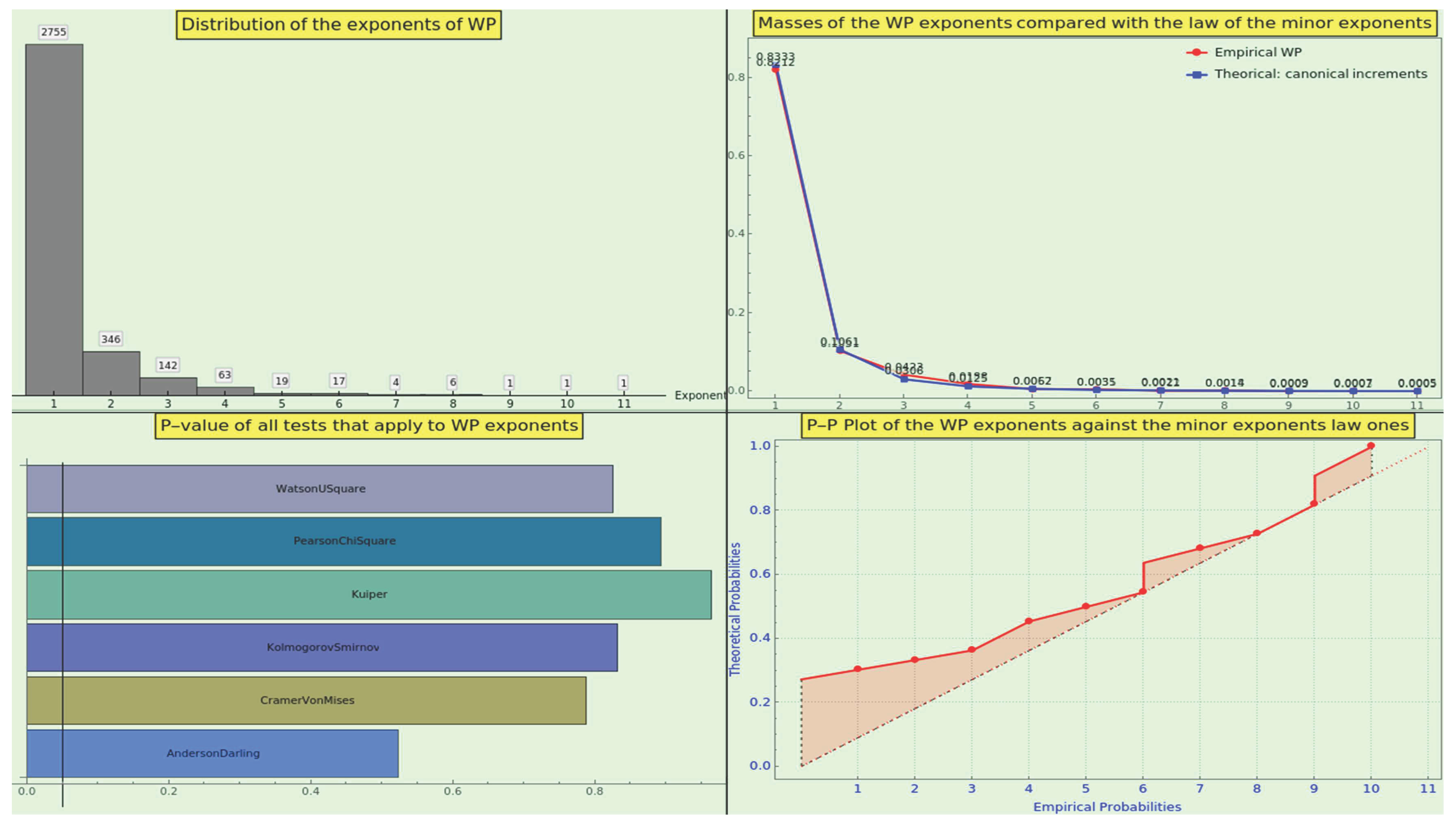
Figure 46.
The LPEs of WP reach the multiplicity 11, as indicated by the histogram in the top-left corner. The plot of the frequencies (empirical in red and theoretical in blue), the p-values of the statistical test methods applied, and the P-P plot indicate excellent conformity.
Figure 46.
The LPEs of WP reach the multiplicity 11, as indicated by the histogram in the top-left corner. The plot of the frequencies (empirical in red and theoretical in blue), the p-values of the statistical test methods applied, and the P-P plot indicate excellent conformity.
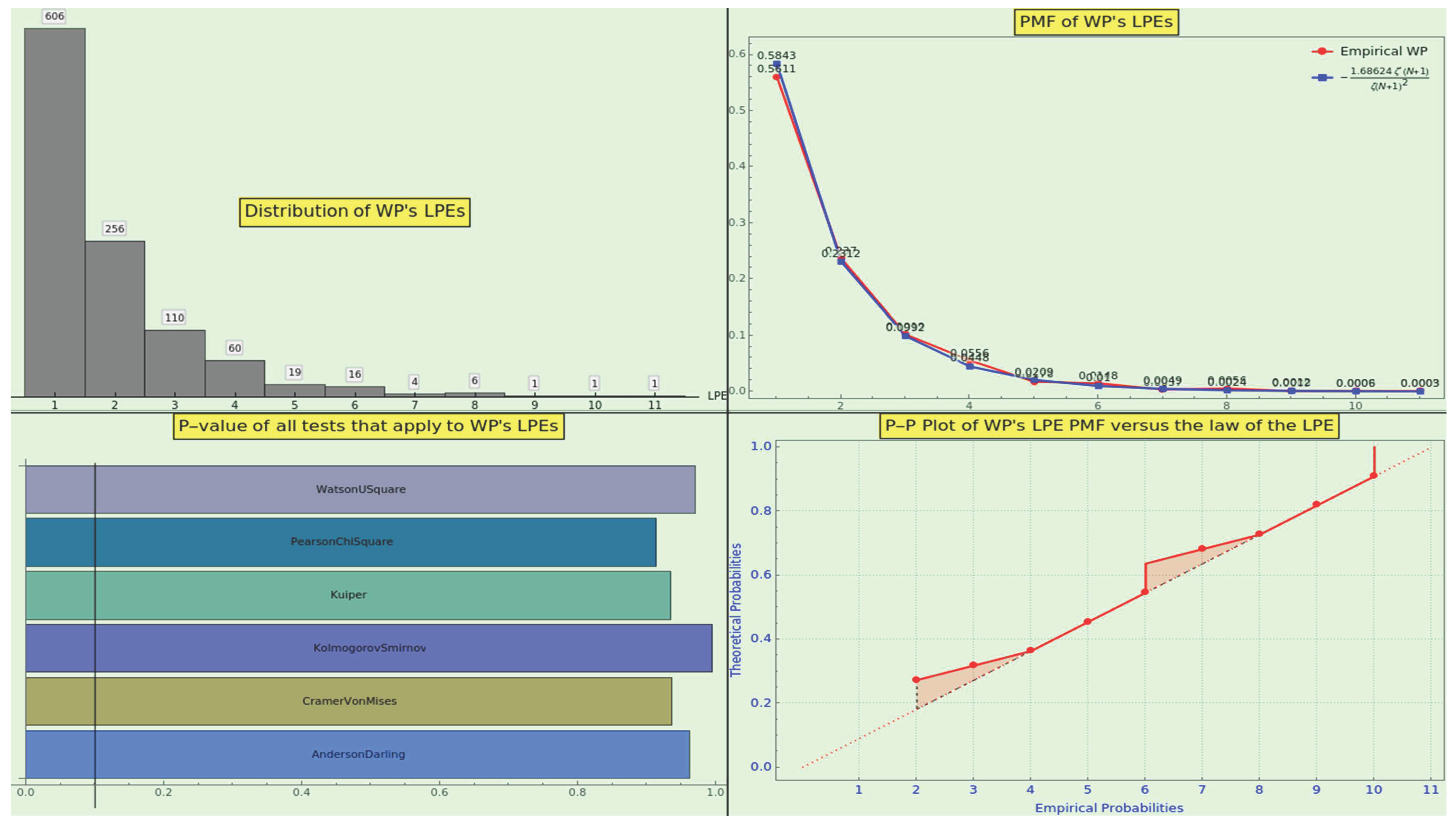
Disclaimer/Publisher’s Note: The statements, opinions and data contained in all publications are solely those of the individual author(s) and contributor(s) and not of MDPI and/or the editor(s). MDPI and/or the editor(s) disclaim responsibility for any injury to people or property resulting from any ideas, methods, instructions or products referred to in the content. |
© 2025 by the authors. Licensee MDPI, Basel, Switzerland. This article is an open access article distributed under the terms and conditions of the Creative Commons Attribution (CC BY) license (http://creativecommons.org/licenses/by/4.0/).
Copyright: This open access article is published under a Creative Commons CC BY 4.0 license, which permit the free download, distribution, and reuse, provided that the author and preprint are cited in any reuse.


