
Submitted:
29 October 2025
Posted:
30 October 2025
Read the latest preprint version here
Abstract
Properly setting the incompressibility constraint for incompressible Navier-Stokes equations has been an area of intense research since the pioneering MAC scheme was proposed in 1965. Nevertheless, the appropriate solution with the pressure Poisson equation in the presence of solid walls has remained an unsolved problem and a controversial topic. This is primarily because the conventional setups often fail to generate a truly solenoidal velocity field (i.e., a velocity field with zero divergence). In the present study, we clarify the longtime misunderstanding of the existing approaches and propose an answer to this problem. A reformulated pressure Poisson equation and its associated Neumann boundary condition are presented. They are derived in detail, analyzed for the pressure compatibility and numerical stability, and then validated successfully with test problems. The new formulations can produce strictly divergence-free velocity solutions to machine accuracy and enhance solution accuracy in general application scenarios. On this basis, we believe the proposed formulations constitute the proper pressure Poisson equation and Neumann boundary condition for solving viscous incompressible flows.
Keywords:
pressure poisson equation
; pressure boundary condition
; incompressible flows
; divergence-free
I. Introduction
The prevailing computational approach of solving viscous incompressible flows employs a pressure Poisson equation (PPE), which offers an efficient means of solving for pressure and velocity either in a coupled manner or separately. Over the years, extensive research endeavors have been dedicated to enhancing the PPE, primarily on three aspects: compatibility, incompressibility, and stability. Compatibility mandates that the source term of the PPE be consistent with the boundary normal pressure gradients within any subdomain. Stability serves to dampen noise arising from numerical errors, since the PPE is not as simple and stable as the heat equation. And incompressibility ensures a divergence-free velocity field from the domain interior to its boundaries. So far, the key challenge lies in the incompressibility in the presence of solid walls. In practical applications, many incompressible wall-bounded flow solutions, even direct numerical simulation (DNS) results, are only ostensibly correct. They are not divergence-free upon close examination, particularly in the vicinity of a solid wall boundary, where the impenetrable boundary does not provide an explicit pressure value and the Neumann boundary condition must be employed. The degraded solutions implicate that many important near-wall flow features, such as the boundary layer stratifications, turbulence structures, flow separations, and corner eddies, may not be accurately predicted. In contrast, converged solutions obtained via the artificial compressibility method can achieve a high degree of solenoidality throughout the domain due to its unique formulation. Therefore, a strictly divergence-free PPE and associated Neumann pressure boundary condition are desired to enable high-fidelity modellings of viscous incompressible flows.
In conventional incompressible flow solvers, the homogeneous Neumann boundary condition, which is derived from the boundary layer theory, is frequently adopted as a convenient approximation for solid wall boundaries.
Despite being simple for implementation and numerically very stable, the accuracy of (1) is confined to scenarios where the local Reynolds number is high. When the normal pressure gradient becomes significant, (1) tends to induce a numerical boundary layer in the near-wall region, corrupting the local velocity field and undermining the flow prediction. Gresho and Sani [1] have presented a numerical example demonstrating that the application of (1) will lead to inaccurate numerical outcomes.
Researchers have also prescribed a Neumann boundary condition based on the momentum equation, in the form of
(2a) is often discretized using ghost points outside of the boundary, where such ghost points are obtained from the continuity relation▽·u = 0. It has very limited stability with an allowable time step much smaller than what the von Neumann analysis indicates. Alternatively, the so-called curl-curl boundary condition [3] (also referred to as the electric boundary condition [4]) is adopted in some research to take account of the tangential velocity component, which is less affected in accuracy by the mesh resolution than the normal component [1]. This boundary condition is also derived from the momentum equation, but it incorporates a normal derivative of the velocity divergence. It is expressed as
Regardless of whether ▽·u is set to zero, (2b) exhibits enhanced numerical stability compared with (2a). Gresho and Sani [1] asserted that (2a) is theoretically consistent with the momentum equation and sufficiently valid for solving the PPE. However, under most circumstances, the Neumann boundary conditions represented by (2) are unable to yield a divergence-free solution. Rempfer [5,6], Henshaw [7,8], and Strikwerda [9] contended that (2) is underdetermined, as it provides no additional information beyond what is already inherent in the interior flow field. Given that no compelling explanations have been put forward to resolve these discrepancies and no consensus has been reached within the research community, the proper specification of the pressure Neumann boundary condition becomes a controversial subject with theoretical ambiguities [1~2, 6].
In pursuit of a divergence-free solution, many follow-up studies have been reported in the literature. These efforts include converting the Neumann boundary condition to the Dirichlet boundary condition [10], enforcing explicit continuity at the boundaries [11], incorporating damping terms [8], prescribed functions [12], supplementary constraints [13], and stabilizing terms [14] to the PPE, as well as proposals of new Neumann pressure boundary conditions [4]. However, the validation cases in some of these studies only presented domain-averaged quantities of the velocity divergence, which are large for coarse grids and tend to decrease to certain nontrivial levels as the mesh is refined. Some researchers attributed this to discretization errors and time increment [15]. This reasoning is misleading because the velocity divergence represents a quantitative relationship between velocity components rather than a primitive variable itself. Similar to the artificial incompressibility method, a well-converged numerical solution with PPE should achieve a zero velocity divergence up to machine precision, irrespective of mesh fineness. By circumventing the Neumann boundary condition, the influence matrix technique developed by Kleiser and Schumann [16] achieves a degree of success. By solving an integral problem for the pressure based on Green’s function in the context of spectral methods, it establishes a linear relation between the pressure and the velocity divergence at the boundary, and enables the determination of the boundary value of the pressure (up to an arbitrary constant). Nevertheless, this method is complex to implement for general problems and has not been widely adopted in the CFD community. Therefore, the open question for a divergence-free solution with PPE and the Neumann pressure boundary condition remains unresolved.
In this paper, we challenge this problem from a new perspective. Theoretically, solving the incompressible flow does not need a pressure boundary condition [2]. But solving a PPE requires a boundary closure. This gives rise to a fundamental contradiction between the theoretical principles and practical numerical implementations. This issue has been largely overlooked in the relevant PPE studies since it was first employed by the MAC method. Accordingly, we argue that those previous viewpoints on (2) being underdetermined are wrong. On the contrary, setting a pressure boundary condition like (1) and (2) makes the system overdetermined. Equations being over-constrained or ill-posed is the reason behind the non-divergence-free velocity field. To resolve the contradiction between the theoretical requirement and practical needs in solving the PPE, our strategy is to set up a temporary pressure boundary condition. It first facilitates the numerical computation of the PPE and then gradually fades away to make the system well-posed. The new PPE and Neumann pressure boundary condition are derived in Section II. They are examined for compatibility, well-posedness, and stability in Section III. Numerical tests are carried out to validate the proposed method, and comparative studies are performed against existing numerics in Section IV, proving the effectiveness and superiority of the new formulations. Summary and conclusion are given in Section V.
II. Theoretical Reformulations
2.1. PPE Reformulations
In conventional PPE solution procedures, the pressure field is uniquely determined by the velocity field of the same moment, independent of the flow’s time history [17]. Some researchers have pointed out that this characteristic constitutes an advantage facilitating the realization of high-order solutions in time [18]. For incompressible flows, the pressure is also considered a Lagrange multiplier to satisfy the continuity constraint, rendering the pressure merely an auxiliary function to correct the velocity field. While these observations may be correct in mathematics, they do not contribute effectively to the proper solution of the pressure field. Orszag et al. [20] have criticized the “parabolic” PPE scheme, saying that it forgets the effect of initial conditions immediately and only reflects the effect of boundary conditions at the domain edge. In his review paper [5], Rempfer has proposed that “the value of the pressure at any point in space and time does not only depend on the value of the velocity field everywhere in the domain; it also depends on its history in time.” As discussed in the last chapter, the boundary-condition-free requirement for PPE necessitates the pressure field being corrected from the one in the last iteration.
Inspired by these thoughts, we aim to reformulate the PPE and the Neumann boundary conditions in this study to incorporate the pressure field from the preceding iteration. The momentum equation for viscous incompressible flows in conservation form is
in which the velocity u = (u(x, y, z), v(x, y, z), w(x, y, z)), ν being the kinematic viscosity and f the body force per unit mass acting on the fluid. Taking the divergence of (3) with the velocity dilatation rate
we can obtain (5) without assuming Ф = 0
With nonzero Ф, (5) can be considered a PPE of the velocity field, which is not converged and solenoidal. When the divergence-free condition is satisfied, we should have Ф = 0 and ∂Ф/∂t = 0 throughout the domain, and (5) becomes
(6) is the so-called standard PPE documented in the literature and can be considered the PPE for the solenoidal velocity field. By comparing (5) and (6), we notice that the velocity source term –(▽u):(▽u)Tand the body force term ▽·f are the common components in both equations. The two PPE only differ by the Ф terms. By eliminating the common terms on their RHS, (5) and (6) suggest a revised PPE in an iterative scheme, with k denoting the iteration index and n+1 referring to the time level at t+∆t.
For steady-state computations using a time-marching approach with unity density, (7a) is simplified as
The viscous term in (7b) conserves the velocity diffusion. Though it produces negligible difference in the solutions, it can boost numerical stability and permit larger pseudo time steps in the computation. The Ф convective term in (7b) is necessary for convection-dominated flows when PPE is directly coupled with the momentum equations. The temporal Ф term in (7b) is indispensable and can be approximated by
In standard PPE practice since its introduction by Harlow and Welch [19], Фn+1 is set to zero to enforce continuity, while Фn is retained as nonzero to maintain numerical stability. When additional Ф terms are involved in (7b), our experience shows that three approaches are viable for handling the temporal Ф terms in (8): retaining both terms, removing both, or retaining only Фn+1. Notably, removing both terms leads to slow convergence with occasional instability, whereas retaining only Фn+1 yields the fastest convergence. And the diffusion term can be evaluated at either time level n or n+1, depending on the computational needs.
Compared with the conventional PPEs of (5) or (6), the new PPE (7) includes only Ф terms on its RHS, eliminating the need to calculate the velocity source term and the divergence of the body force f. The influence of f on pressure is instead accounted for in the momentum equation calculations. The iterative nature of (7) establishes a mechanism that drives the Ф field towards zero during the pressure evolution. Once Ф converges to a trivial value, (7) becomes equivalent to the continuity equation. The use of the variable Ф avoids the direct coupling between the pressure and the velocity, and moderates the pressure updating through its spatial distribution, transport, and diffusion. A similar technique was employed in the pressure gradient method study [21] to achieve divergence-free solutions without the need for specifying pressure gradient boundary conditions. Since |Ф| << 1 typically holds in the domain interior, the nonlinear terms and viscous terms in (7b) are generally small in magnitude. Defining P’ = Pn+1– Pn, (7b) retaining only the temporal term, is simplified as
This approximates the corrective PPE used in the well-known SIMPLE method, in which zero velocity divergence is assumed at the next iteration and Ф represents the velocity dilatation of the intermediate velocity field. Therefore, the theoretical soundness of (7b) is partially validated by the proven success of the SIMPLE algorithm. And the viscous terms in (7b) can be extended to the SIMPLE series method and the projection methods to improve numerical stability. However, it should be noted that (7c) can only be solved separately from the momentum equation as in the SIMPLE algorithm, due to its lack of the Ф convection term required for mass transport.
2.2. Corrective Pressure Boundary Condition
Boundary condition specification for the pressure is required for solving (7), particularly the Neumann boundary condition for wall-bounded flows. As discussed in Section I, directly applying the conventional boundary condition of (2) will not yield a divergence-free solution, though it is theoretically consistent with the Navier-Stokes equations. We rederive the pressure gradient expression from the momentum equation (3) with all Ф terms retained as
or
in which ω=▽◊u is the curl. (9b) can be interpreted as the Neumann pressure boundary condition when Ф≠0 and the flow field is non-solenoidal prior to convergence. When Ф=0, the above equation corresponds to the converged and solenoidal flow field, taking the form:
Following the same methodology used in deriving (7), we combine (9b) and (9c) and obtain an evolving Neumann boundary condition in an iterative scheme with time marching.
Compared with boundary conditions (1) and (2), (10) involves only 1st-order derivatives, incorporates the tangential velocity effects through the Ф term, and imposes no larger complexity in implementation. It is evident that this boundary constraint will be weakened as Ф gets close to zero globally, making the system well-posed. This is the same principle as the artificial compressibility method and (7): the boundary pressure update will diminish when Ф is approaching zero. (10) also accounts for the influence of the wall normal velocity via the unФ term. With respect to the numerical compatibility, we have found that this boundary condition (10) alone will not produce a divergence-free solution without coupling with the new PPE (7), as will be shown in Section IV. For implementations, the normal derivatives of P and Ф can utilize one-sided spatial discretization schemes of any high order. This new pressure boundary condition can also be promoted to the SIMPLE family to achieve divergence-free solutions and to the artificial compressibility method. Orszag et al. [20] have proposed an iterative Neumann pressure boundary condition in a similar form to (10) for high-order temporal accuracy, without providing any derivations and numerical validation. But their formulation features an undetermined parameter and misses the un term for wall normal speed.
Since the calculation of (7) and (10) needs the Ф values at the boundaries, the boundary condition for Ф is equally critical. The boundary Ф specification must be numerically consistent with the interior Ф calculation to make the Ф field continuous and smooth in the computation. For wall-bounded flows, setting Ф directly to zero at wall boundaries skips the non-solenoidal evolution process and may fail to yield a divergence-free solution. A Rubin boundary condition for Ф has been proposed in [22] using the energy method. It is equivalent to setting ∂Ф/∂n = 0 at the stationary solid wall boundary. It is not compatible with (10), because ∂Ф/∂n = 0 implies a constant ∂P/∂n in (10) from its initial value at the boundaries. Therefore, we adopt the Dirichlet boundary condition for Ф on solid walls and compute it with (4) and one-sided difference scheme.
On a staggered mesh, the computation of the Ф field should be simple and straightforward. However, for collocated mesh, the pressure and Ф field solutions have been observed in numerical experiments with some spurious oscillations near certain solid walls. They stem from the numerical discontinuities between the interior and the boundary Ф values, introduced by the artificial viscosity term used to supplement the central scheme for interior Ф computations. When the magnitude of Ф diminishes, any non-decaying numerical errors become significant, contaminating the domain and causing solution wiggles. As we know, an upwind or one-sided scheme can be decomposed into one symmetrical part and one antisymmetric part. Conversely, the antisymmetric central scheme augmented with a symmetric artificial viscosity term is equivalent to an upwind or one-sided scheme. For illustration, consider a finite difference central scheme (CS) with uniform grid spacing ∆x, defined as
and a typical 4th-order artificial viscosity term (AVT) as
As shown in (12), a 3rd-order forward/backward one-sided scheme (used for the left/right boundary) can be expressed as a linear combination of the above CS and AVT terms. In practice, however, these combinations typically involve terms of different orders and include a scaling coefficient.
The backward one-sided scheme (12b) for boundaries with ending coordinate indices equals CS + AVT. This is the same combination used in the domain interior to compute ∂u/∂x for Ф. In contrast, the forward one-sided scheme (12a) for boundaries with starting coordinate indices conflicts with CS + AVT, being responsible for the oscillatory Ф field near these boundaries. Though the numerical schemes (including compact schemes) applied in implementations may be different, the core inconsistency between boundary and interior discretizations persists. The artificial dissipation term can be gradually removed with an exponentially decaying coefficient as performed by Rogers et al. [23], but the decaying parameter requires some case-by-case tuning, making this technique not very feasible.
We have found a simple technique to resolve this inconsistency. As pointed out by Mazumder [24], in a physical problem, when a boundary derivative (e.g., ∂un/∂n) is not a prescribed value but computed with one-sided schemes, additional numerical error other than the truncation error will arise. And the solution of this derivative will be discontinuous from the interior to the boundaries, because the governing equation is not satisfied at the boundary. Mazumder has provided a corrective treatment: enforce the governing equation in the one-sided scheme for 1st-order derivatives by incorporating a 2nd-order derivative, which may be already known from the physical problem. For one-dimensional implementation with uniform grid spacing ∆x, a 2nd-order derivative can be embedded into the one-sided difference scheme for the 1st-order u derivative by cancelling the 3rd-order derivatives in the following two Taylor series expansions:
so that
In computing ∂un/∂n for (4), the 2nd-order term ∂2un/∂n2 is accessible in the momentum equation in the form of (2) and can be replaced with (∂P/∂n)/μ for a solid wall boundary. Therefore, Ф at the wall boundary with the starting coordinate index is computed as
By replacing the d²u/dx² term with the pressure gradient, (15a) establishes a new local coupling that improves numerical accuracy and convergence rate. Though (2) should not be used as a proper boundary condition to solve PPE, it is still a useful relation in this treatment. For finite volume implementations, in which the boundary conditions are applied on the cell faces rather than the cell centers, ∂un/∂n is computed differently. On a one-dimensional grid of equal cell spacing ∆x, Ф at the left (W) wall boundaries (starting coordinate index) is calculated as
with the centers of the boundary cell and the cell next to it denoted as O and E.
Based on the above discussions, we choose to compute Ф with (15) at the boundaries of starting coordinate indices, while employing uncorrected one-sided schemes to calculate Ф at the solid wall boundaries of ending indices. The uncorrected one-sided schemes can be of any order relative to the central scheme for computing the interior Ф. With this implementation on collocated grids, the pressure and Ф fields become very smooth without any wiggles, and we can minimize the Ф magnitude to nearly machine accuracy. Although (15) will turn out to be a 3rd-order one-sided scheme if the d²u/dx² term is substituted with a one-sided discretization, this 3rd-order scheme will not work as effectively as (15). And if we apply the correction procedure to the opposite one-sided scheme for wall boundaries of ending indices, the Ф solution will be a uniform nontrivial value, since the correction disrupts the prior CS + AVT consistency.
For non-solid wall boundaries, such as an inflow with a static pressure value and a domain symmetry with zero pressure gradient, the theoretical requirement of avoiding explicit pressure boundary conditions is violated. In these cases, the solution of the PPE (7) should be restricted to the domain interior and solid wall boundaries. For inflow or outflow boundaries, Ф can be set to zero, assuming the far-upstream or far-downstream flows satisfy the continuity as in fully developed or undisturbed regions. This treatment maintains consistency with the iterative evolution of Φ toward zero in the domain interior.
III. Compatibility, Well-Posedness, and Stability Analysis
This section will examine the PPE and Neumann boundary condition formulations proposed in the last section for specific theoretical validity and numerical stability, prior to proceeding with code implementations and computer testing. It is widely recognized that the pressure field is conservative, and a valid pressure solution must satisfy the divergence theorem within the domain or any subdomain as a compatibility requirement or solvability condition.
For the conventional PPE and pressure boundary condition specified by (2) and (6), the compatibility condition (16) can be readily proved based on their derivations from the momentum equations [13]. For our proposed PPE (7) and pressure boundary condition (10), this relation is less evident due to their incorporation of pressure and pressure gradient corrections.
Proof Within a three-dimensional domain or sub-domain Ω, the loop integral of the normal pressure gradient correction at the boundary can be expressed based on (10) as
Given that ∂Ф/∂n in (17) is continuous and differentiable, we can directly derive the following result from the divergence theorem:
Considering unФ in (17) also being a vector and the definition ▽·u = Ф, we have again from the divergence theorem that
Combining (17), (18) and (19), we obtain
Comparing with (7), we have arrived at
As and in the time marching process, we have
With a 1st-order Euler’s backward time differencing assumption, the summing term in (22) is
When the initial value Ф0 is zero and the converged Фn equals zero, or with n and 0 representing two time instants of a solenoidal flow field, (23) will become zero. Therefore, the compatibility requirement for the pressure solution (16) holds analytically for our proposed PPE and pressure boundary conditions provided the computation converges. □
The numerical stability and specific stable conditions are another concern for the proposed PPE formulations and pressure boundary condition on solid walls. The existing stability analysis techniques applicable to general initial-boundary-value problems include the summation-by-parts (SBP) energy method [25], simultaneous approximation term (SAT) method [26], pseudospectra method [27], and the normal mode analysis [28]. In this study, the numerical well-posedness and stability of the aforementioned formulation are examined utilizing the normal mode analysis. This method is a generalization of the von Neumann stability analysis to account for the influence of nonperiodic boundary conditions. We study a two-dimensional Stokes problem in steady state for simplicity. It has been proved in [29] that the predictions from the normal mode analysis for the Stokes equations are also applicable to the full Navier-Stokes equations. The conventional pressure boundary conditions of (2a) and (2b) have been investigated via the normal mode analysis by Petersson [3] and Zhang et al. [30] in semi-discrete or fully discrete form with different time schemes. For our proposed PPE and pressure boundary condition, we consider the semi-discrete form by discretizing the time term and leaving all the spatial terms continuous. The Stokes problem is defined by the equations and boundary conditions presented in (24), within a finite domain Ω with periodicity over (0, 2π) in x-direction and solid wall boundaries at the two ends of [-1, 1] in y-direction. Assuming a forward Euler scheme, we replace the iterative relation in PPE (7b) and pressure boundary condition (10) with a time derivative and a constant time step ∆t as in a time marching procedure. The convective terms in (7b) are absent in the Stokes flow, and the insignificant nonlinear terms in (7b) are neglected to facilitate the analysis.
With a uniform mesh of grid spacing ∆x = 2π/N, we consider a discrete Fourier transform of a grid function F (x, y) as
where i is the square root of -1. The wave numbers ω = 0 ~ N-1 correspond to a complete set of eigenfunctions eiωx within the mesh domain. We perform a Fourier transform of the solution in the x-direction and make the ansatz for differential equations (24) in semi-discrete form as
By employing fully implicit momentum equations and an explicit expression for Ф, we can derive the eigenvalue problem (27) by neglecting the forcing term and assuming unity density. The Godunov-Ryabenkii condition states that the solution to the system (24) is unstable if the eigenvalue κ of (27) exists and |κ| > 1.
By substituting , (27) without boundary conditions can be simplified as
Without having to solve for u and v, the admissible odd solutions for the pressure and Ф are
By substituting the above pressure and the Ф solutions into the pressure boundary condition (27e) at y = ±1, we can obtain an explicit and real expression for κ as
From (30), it can be readily verified that |κ| < 1/2 for any nonnegative wave number ω, which is defined by the discrete Fourier transform (25). This confirms that the proposed formulation is unconditionally stable and this problem is well-posed in the strong sense. A similar conclusion holds for the even solutions. In the above analysis, no u velocity specification is required at the wall boundary y = ±1. Therefore, this analysis also applies to slip or non-slip moving wall boundaries. This special benefit has not been found in prior normal mode analysis on incompressible flow equations [3,29,30].
IV. Numerical Examples
In this section, the proposed PPE and Neumann boundary condition are validated with two-dimensional steady-state laminar flow problems. Eqs. (3), (4), and (7) are solved simultaneously using the finite difference method. All convection and diffusion terms are discretized with second-order central schemes on collocated grids. Artificial viscosity is thus added for the pressure gradient terms in (3), the velocity gradient terms in (4), and the Ф transport terms in (7). The time derivative is discretized by the backward Euler scheme. And the pressure field is regularized to a zero mean value after each iteration. No convergence acceleration technique is employed to preserve all the solution details. The flow domains are initialized with a uniform pressure field and a static velocity field. However, we have found that initial velocity and pressure fields of random but moderate values, which make the initial flow field non-divergence-free, also yield satisfactory results. Because the computation can rapidly purge out the randomness in the iterations.
4.1. Lid-Driven Cavity Flow
The first validation case is the classic top-lid-driven cavity flow. This wall-bounded flow is simple in geometry but rich in flow features. The square domain consists of boundary conditions of all Neumann type for the pressure. It also features numerical singularities at the two upper corners, which often pose difficulties for conventional PPE solutions. This problem is first tested using our proposed formulations on a 129 × 129 mesh. The obtained centerline velocity profile results for different Reynolds numbers are plotted in Figure 1 and compared with the benchmark data of Ghia et al. [31], which are based on the vorticity-stream function method and strictly divergence-free. The two data sets show excellent agreement. Figure 2(a) presents the convergence history for the case with Re = 1000. Figrures 2(b) and 2(c) demonstrate the domain solutions of the velocity dilatation, confirming the capability of our new formulations for producing a genuinely divergence-free velocity field. The resolved magnitude level of Ф is independent of the grid spacing. And it is not affected by the corner singularity from the domain geometry. We have also noticed that before Ф converges to the level of nearly machine zero, its contours bear a rough resemblance to the pressure contours. This Ф-P quantitative relationship can be described by the penalty method. Although the artificial viscosity involved in computing (4) may be nontrivial in certain regions, it does not compromise the fact that this formulation is able to drive the given Ф expression to near machine zero.
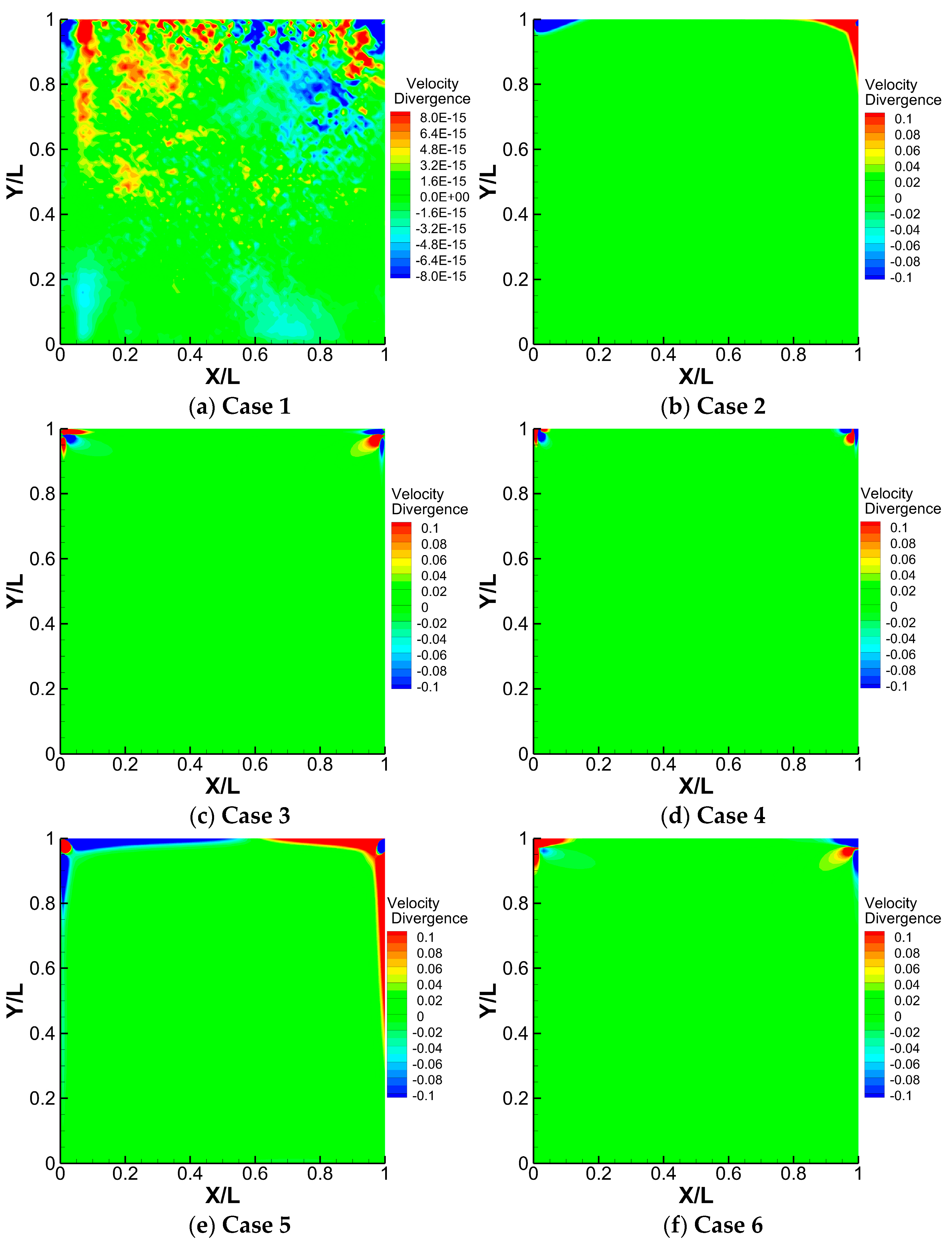
We then conducted a comparative study in numerics with this cavity flow problem on a 101× 101 mesh. Table 1 elaborates the case setup employing the PPE and pressure boundary conditions from the proposed method, previous methods, and their mixtures. We also examine the curl-curl and the homogeneous pressure boundary conditions in this study. All cases utilize identical formulations except for the PPE and pressure boundary condition. For Cases 2 and 3, the discretization of (2a) includes ghost points computed by applying the continuity equation at the boundary. For Case 4, the boundary vorticity is calculated for the curl-curl boundary condition (2b). Table 1 also lists the maximum stable time step sizes in serial computing for comparison, with equal underrelaxations in variable updating for each case. The well-converged velocity divergence solutions for Case 1~6 are presented in Figrures 3(a)~(f). It is evident that our proposed PPE and pressure boundary condition outperform the others and represent the only combination capable of achieving divergence-free solutions (Case 1). The rest of the cases exhibit high magnitudes of velocity dilatation up to the level of ~102 near the two upper corners, which exceed typical numerical errors and indicate poor solution quality under the influence of boundary singularities. To better visualize the solution differences, the contour range for Case 2 to 6 is restricted to -0.1 ~ 0.1. The conventional PPE with the homogeneous pressure boundary condition yields the poorest result, as it additionally produces numerical boundary layers adhering to the two side walls. We also find that our proposed boundary condition (10) alone will not generate divergence-free solutions with the conventional PPE (Case 6), nor will our proposed PPE perform well with the conventional boundary condition (Case 2). Because the pressure correction in (7b) and (10) should be consistent between the domain interior and boundaries.
From the time step comparison in Table 1, our proposed PPE and boundary condition (Case 1) demonstrate a significant advantage in stability over the conventional setups (Case 3 and Case 4), albeit Case 4 is also theoretically proven unconditionally stable [6]. For this problem, our new PPE functions adequately with only the linear terms in (7b), and its stability is considerably enhanced when more nonlinear terms are included. Without external ghost points from the continuity, Cases 2 and 3 will have even smaller allowable time steps. The homogeneous pressure boundary condition (Case 5) permits the largest time steps. This is attributed to its numerical simplicity, which enhances the diagonal dominance of the system matrix. From these comparisons, the pressure solutions for Case 2~5 are uniquely determined but flawed. Based on the PDE theory, we conclude that the pressure boundary conditions ((1) and (2)) are enforced excessively, making the system ill-posed instead of being underdetermined as previously hypothesized. The homogeneous pressure boundary condition (Case 5) imposes the most rigid over-constraint and consequently renders the largest errors.
Figure 3.
Velocity divergence solutions with the problem setup prescribed in Table 1 for Re = 100 on a 101 x 101 uniform mesh.
Figure 3.
Velocity divergence solutions with the problem setup prescribed in Table 1 for Re = 100 on a 101 x 101 uniform mesh.
4.2. Flow Passing a Circular Cylinder
The second validation case focuses on the uniform flow passing a circular cylinder. It is a fundamental external flow problem characterized by flow separation and wake formation. The accurate prediction of these flow features heavily relies on the velocity solution quality and the proper specification of the pressure boundary condition on the cylinder surface. This problem is investigated under steady-state condition at a Reynolds number of 40. As illustrated in Figure 4, the cylinder diameter is set to unity, and the circular computational domain is designed with a radius 25 times the cylinder diameter to mitigate the adverse influence of the finite domain effects on flow predictions. The 541 × 301 structural mesh is clustered around the cylinder and refined in the wake region to better capture the flow details. The near wake region has a radial resolution of 0.01. And all intersecting mesh lines are configured to be orthogonal to one another to reduce discretization errors. The external boundary condition configurations for each variable are also specified in Figure 4. The left semicircle of the domain serves as the inflow boundary with given velocity, static pressure, and Ф. The right semicircle functions as the outflow boundary with the velocity and pressure values obtained by streamwise extrapolation from the domain interior.
As outlined in Table 2, the simulations are carried out using our proposed PPE/pressure boundary condition and the conventional formulations for comparative study. All cases are run with identical time-marching durations to ensure sufficient convergence. The experimental measurements by Coutanceau and Bouard [32] are available as baseline data on the flow separation angle and reattachment distance. Solution flow fields from the three simulations are visualized in Figure 5 with streamlines and velocity divergence contours. Our proposed PPE and boundary condition produce a high-level divergence-free solution (Figure 5(a)). If more iterations are executed, the velocity divergence magnitude can be further reduced. For conventional PPE and boundary condition (Figure 5(b)), the velocity divergence reaches a level of 10-2. And for conventional PPE with a homogeneous boundary condition (Figure 5(c)), this magnitude increases to the level of 10-1, with high values concentrated round the cylinder surface.
Table 2 compares the separation angle (θ) and the reattachment distance measured from x = 0 as defined in Figure 5(a) for the three cases. The flow separation point on the cylinder surface and the reattachment point are identified by streamline bifurcations. Our proposed formulation predicts the reattachment distance closest to the experimental measurement, whereas the conventional PPE with homogeneous pressure boundary condition results in the largest deviation. For the separation angle, results of all three cases are very close. They differ from the experimental data by approximately 1 degree, partly attributed to the mesh resolution. This numerical example demonstrates that the correct pressure boundary condition and divergence-free velocity solution are critical in the flow separation prediction, which in turn influences wake length and drag estimates. Our proposed formulations thus provide an important improvement in this predictive capability.
Figure 6 compares the pressure and normal pressure gradient on the upper half-cylinder surface along the central angle, which starts from the rear stagnation point. In Figure 6(a), Case 1 and Case 2 display nearly identical pressure curves, while the curve of Case 3 is slightly smaller in magnitude. Overall, their predictions are in close agreement. That also indicates very similar tangential pressure gradients along the cylinder surface. However, differences between the three cases become more pronounced for the normal pressure gradients, which are post-processed from the pressure solutions using a one-sided scheme. Case 1 resolves a peak normal pressure gradient approximately 10% larger than Case 2, whereas the pressure gradient in Case 3 is trivial due to constraints imposed by its simulation setup. A comparison of Figrures 6(a) and (b) reveals that nearly identical boundary pressure values can correspond to distinct normal gradients, which subsequently impact both pressure and velocity solutions. This observation casts doubt on the validity of the practice adopted by some researchers [10,16], namely, replacing the Neumann pressure boundary condition on solid walls with a Dirichlet boundary condition, even if the Dirichlet-specified pressure values are accurate. Based on the curl-free relationship for the pressure gradients, ∂Pn/∂τ = ∂Pτ/∂n, this distinction in normal pressure gradients also accounts for the difference in tangential pressure gradients next to the wall surface, which subsequently affects the flow separation predictions.
V. Conclusions
On the open question of properly specifying the Neumann pressure boundary condition for PPE, this study clarifies some long-time misconceptions and proposes a reformulated PPE and corresponding Neumann boundary condition. The new formulation computes the pressure through an iterative process and can generate a genuinely divergence-free solution in the presence of static or moving wall boundaries. It is simple to implement, contains no undetermined coefficient, and can be extended to time-dependent modeling via the dual-time stepping technique. It also holds potential for integration into the SIMPLE family methods and projection methods to improve solution quality. The formulation is examined for its compatibility with the pressure field, well-posedness, and numerical stability. The numerics are validated successfully with two test cases. It is also compared with the existing PPE and multiple conventional Neumann pressure boundary conditions, showing enhanced stability and accuracy, which is rooted in its adherence to the PDE theory. By this study, we have harvested a new understanding of the PPE methodology and resolved the conflict between the theoretical well-posedness demand for no pressure boundary condition and the boundary closure for PPE. We hope this study will help settle the debate regarding the pressure boundary conditions and deepen our insight into solving the viscous incompressible flows with primitive variables.
This research did not receive any specific grant from funding agencies in the public, commercial, or not-for-profit sectors.
Declaration of Interest Statement
The author declares no competition of interest.
References
- Gresho, P.M.; Sani, R.L. On pressure boundary conditions for the incompressible Navier-Stokes equations. Int. J. Numer. Methods Fluids 1987, 7, 1111–1145. [Google Scholar] [CrossRef]
- Sani, R.L.; Shen, J.; Pironneau, O.; Gresho, P.M. Pressure boundary condition for the time-dependent incompressible Navier–Stokes equations. Int. J. Numer. Methods Fluids 2005, 50, 673–682. [Google Scholar] [CrossRef]
- Petersson, N. Stability of Pressure Boundary Conditions for Stokes and Navier–Stokes Equations. J. Comput. Phys. 2001, 172, 40–70. [Google Scholar] [CrossRef]
- Rosales, R.R.; Seibold, B.; Shirokoff, D.; Zhou, D. High-order finite element methods for a pressure Poisson equation reformulation of the Navier–Stokes equations with electric boundary conditions. Comput. Methods Appl. Mech. Eng. 2021, 373. [Google Scholar] [CrossRef]
- Rempfer, D. On Boundary Conditions for Incompressible Navier-Stokes Problems. Appl. Mech. Rev. 2006, 59, 107–125. [Google Scholar] [CrossRef]
- Rempfer, D. Two remarks on a paper by Saniet al. Int. J. Numer. Methods Fluids 2008, 56, 1961–1965. [Google Scholar] [CrossRef]
- Henshaw, W.D. A Fourth-Order Accurate Method for the Incompressible Navier-Stokes Equations on Overlapping Grids. J. Comput. Phys. 1994, 113, 13–25. [Google Scholar] [CrossRef]
- Henshaw, W.D.; Kreiss, H.-O.; Reyna, L.G. A fourth-order-accurate difference approximation for the incompressible Navier-Stokes equations. Comput. Fluids 1994, 23, 575–593. [Google Scholar] [CrossRef]
- Strikwerda, J.C. Finite Difference Methods for the Stokes and Navier–Stokes Equations. SIAM J. Sci. Stat. Comput. 1984, 5, 56–68. [Google Scholar] [CrossRef]
- Abdallah, S.; Dreyer, J. Dirichlet and Neumann boundary conditions for the pressure poisson equation of incompressible flow. Int. J. Numer. Methods Fluids 1988, 8, 1029–1036. [Google Scholar] [CrossRef]
- Johnston, H.; Liu, J.-G. Finite Difference Schemes for Incompressible Flow Based on Local Pressure Boundary Conditions. J. Comput. Phys. 2002, 180, 120–154. [Google Scholar] [CrossRef]
- Bonfigli, G. Numerical solution of the incompressible Navier-Stokes equations with explicit integration of the pressure term. PAMM 2007, 7, 4100019–4100020. [Google Scholar] [CrossRef]
- Shirokoff, D.; Rosales, R. An efficient method for the incompressible Navier–Stokes equations on irregular domains with no-slip boundary conditions, high order up to the boundary. J. Comput. Phys. 2011, 230, 8619–8646. [Google Scholar] [CrossRef]
- Vreman, A. The projection method for the incompressible Navier–Stokes equations: The pressure near a no-slip wall. J. Comput. Phys. 2014, 263, 353–374. [Google Scholar] [CrossRef]
- Sotiropoulos, F.; Abdallah, S. The discrete continuity equation in primitive variable solutions of incompressible flow. J. Comput. Phys. 1991, 95, 212–227. [Google Scholar] [CrossRef]
- Kleiser, L.; Schumann, U. Treatment of Incompressibility and Boundary Conditions in 3-D Numerical Spectral Simulations of Plane Channel Flows. Proceedings of the Third GAMM-Conference on Numerical Methods in Fluid Mechanics. Notes on Numerical Fluid Mechanics 1980, 2, 165–172. [Google Scholar] [CrossRef]
- Pope, S.B. Turbulent Flows; Cambridge University Press: Cambridge, UK, 2000. [Google Scholar] [CrossRef]
- Zhang, Q. GePUP: Generic Projection and Unconstrained PPE for Fourth-Order Solutions of the Incompressible Navier–Stokes Equations with No-Slip Boundary Conditions. J. Sci. Comput. 2015, 67, 1134–1180. [Google Scholar] [CrossRef]
- Harlow, F.H.; Welch, J.E. Numerical Calculation of Time-Dependent Viscous Incompressible Flow of Fluid with Free Surface. Phys. Fluids 1965, 8, 2182–2189. [Google Scholar] [CrossRef]
- Orszag, S.A.; Israeli, M.; Deville, M.O. Boundary conditions for incompressible flows. J. Sci. Comput. 1986, 1, 75–111. [Google Scholar] [CrossRef]
- Li, Z.; Li, Y. An improved pressure gradient method for viscous incompressible flows. Comput. Fluids 2024, 285. [Google Scholar] [CrossRef]
- Nordström, J.; Mattsson, K.; Swanson, C. Boundary conditions for a divergence free velocity–pressure formulation of the Navier–Stokes equations. J. Comput. Phys. 2007, 225, 874–890. [Google Scholar] [CrossRef]
- Rogers, S.; Kwak, D.; Kaul, U. On the accuracy of the pseudocompressibility method in solving the incompressible Navier-Stokes equations. Appl. Math. Model. 1987, 11, 35–44. [Google Scholar] [CrossRef]
- Mazumder, S. Numerical Methods for Partial Differential Equations: Finite Difference and Finite Volume Methods; Academic Press, 2016. [Google Scholar]
- Svärd, M.; Nordström, J. Review of summation-by-parts schemes for initial–boundary-value problems. J. Comput. Phys. 2014, 268, 17–38. [Google Scholar] [CrossRef]
- Carpenter, M.H.; Gottlieb, D.; Abarbanel, S. Time-Stable Boundary Conditions for Finite-Difference Schemes Solving Hyperbolic Systems: Methodology and Application to High-Order Compact Schemes. J. Comput. Phys. 1994, 111, 220–236. [Google Scholar] [CrossRef]
- Trefethen, L.N.; Embree, M. Spectra and Pseudospectra: The Behavior of Nonnormal Matrices and Operators; Princeton University Press, 2005. [Google Scholar]
- Gustafsson, B.; Kreiss, H.-O.; Sundström, A. Stability theory of difference approximations for mixed initial boundary value problems. II. Math. Comput. 1972, 26, 649–686. [Google Scholar] [CrossRef]
- E, W.; Liu, J.-G. Projection Method II: Godunov–Ryabenki Analysis. SIAM J. Numer. Anal. 1996, 33, 1597–1621. [Google Scholar] [CrossRef]
- Zhang, G.; Cai, M. Normal mode analysis of 3D incompressible viscous fluid flow models. Appl. Anal. 2019, 100, 116–134. [Google Scholar] [CrossRef]
- Ghia, U.; Ghia, K.; Shin, C. High-Re solutions for incompressible flow using the Navier-Stokes equations and a multigrid method. J. Comput. Phys. 1982, 48, 387–411. [Google Scholar] [CrossRef]
- Coutanceau, M.; Bouard, R. Experimental determination of the main features of the viscous flow in the wake of a circular cylinder in uniform translation. Part 1. Steady flow. J. Fluid Mech. 1977, 79, 231–256. [Google Scholar] [CrossRef]
Figure 1.
Centerline velocity profiles for Re = 100, 400, and 1000 on a 129 × 129 mesh.
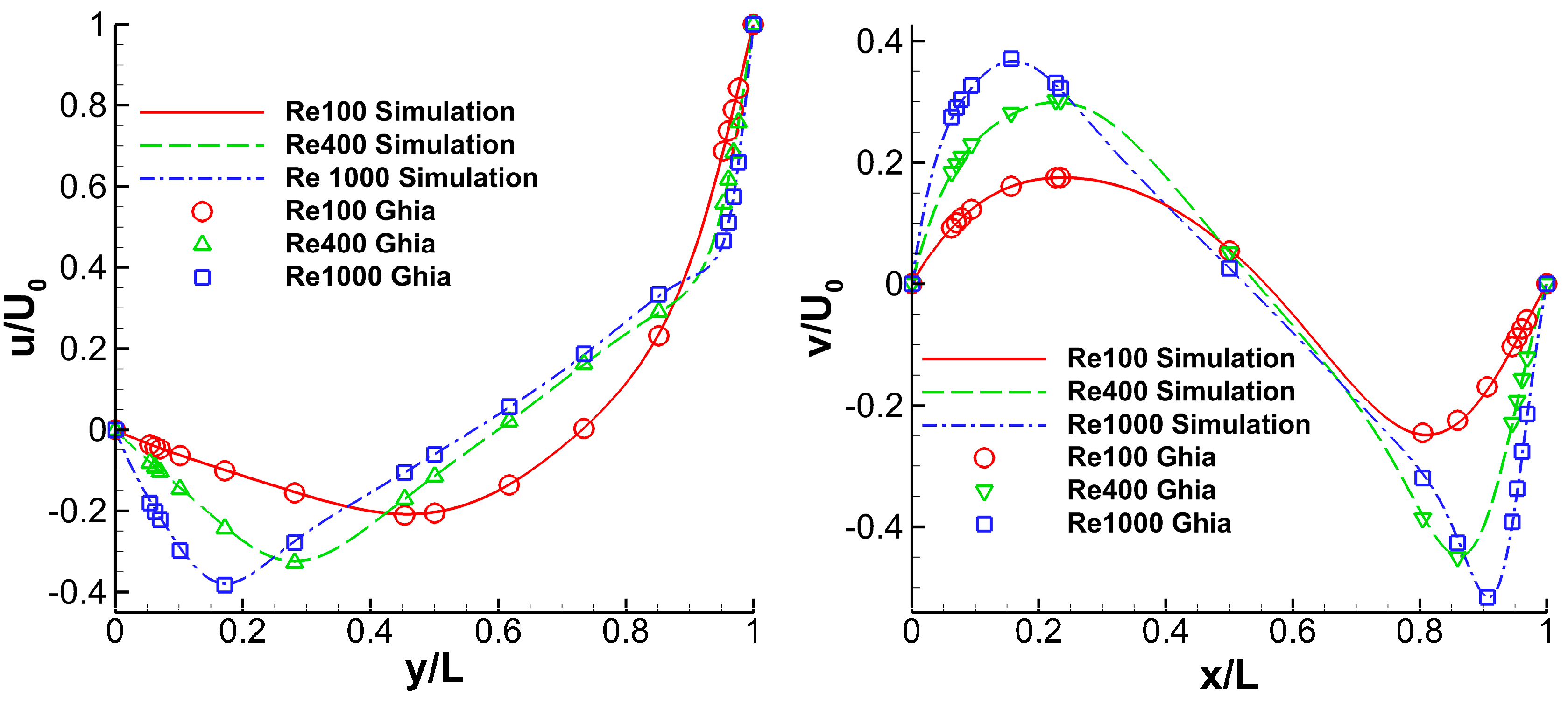
Figure 2.
Simulation results for Re = 1000: (a) l2-norm convergence history (129×129), (b) velocity divergence (81×81), (c) velocity divergence (129×129).
Figure 2.
Simulation results for Re = 1000: (a) l2-norm convergence history (129×129), (b) velocity divergence (81×81), (c) velocity divergence (129×129).
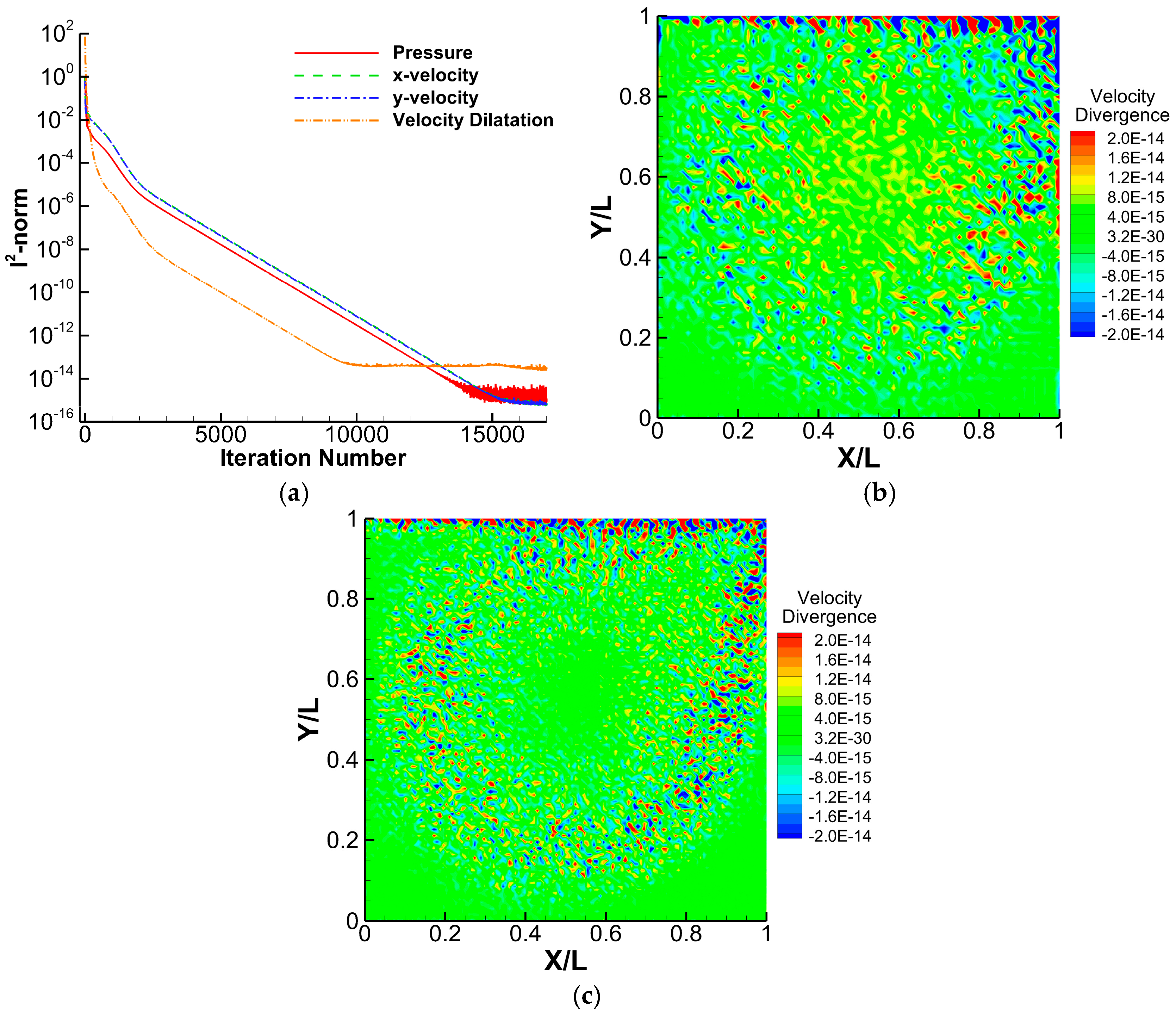
Figure 4.
Computational mesh and external boundary condition setup.
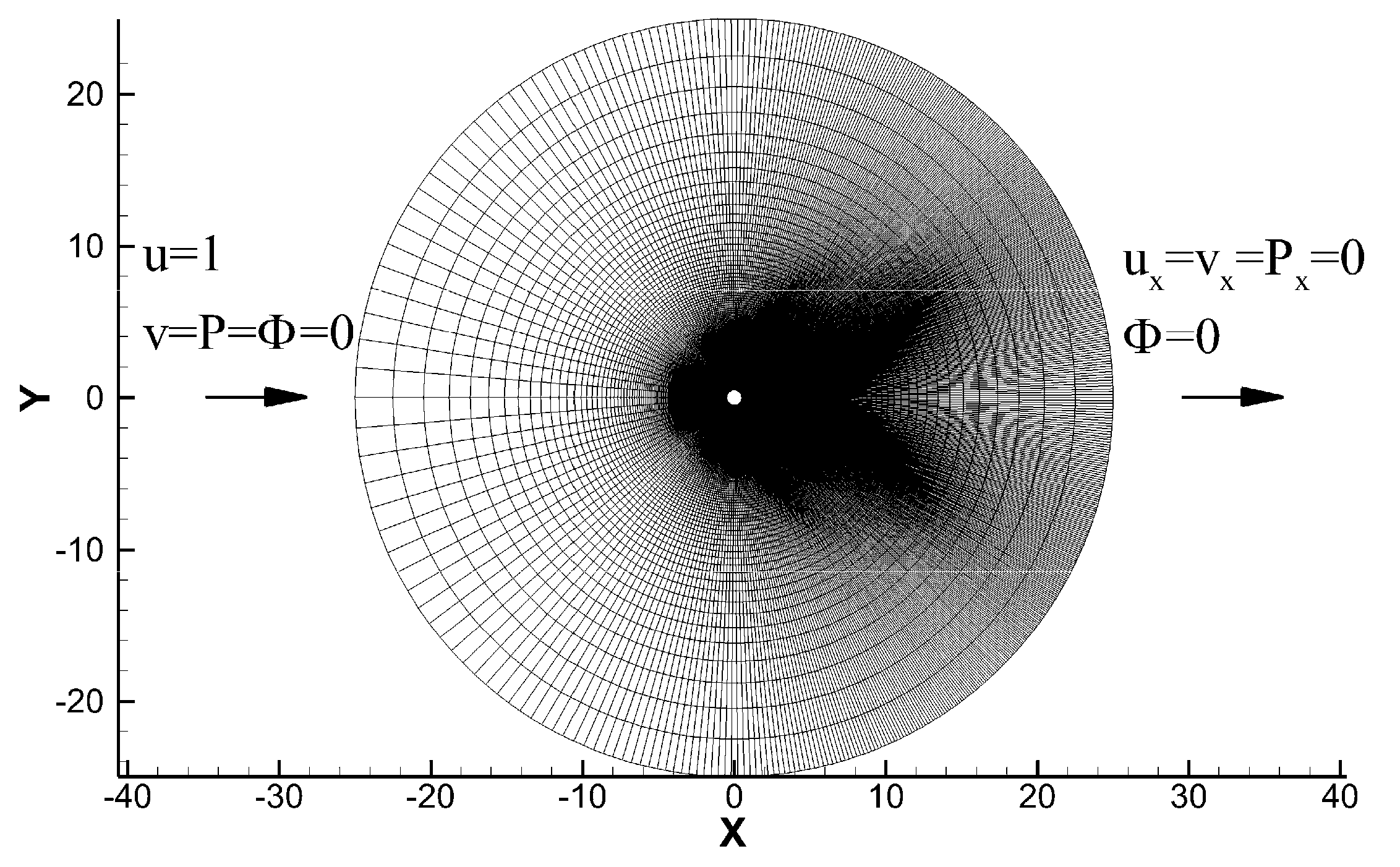
Figure 5.
Velocity divergence with streamlines visualizing the flow separation behind the cylinder from three simulation results.
Figure 5.
Velocity divergence with streamlines visualizing the flow separation behind the cylinder from three simulation results.
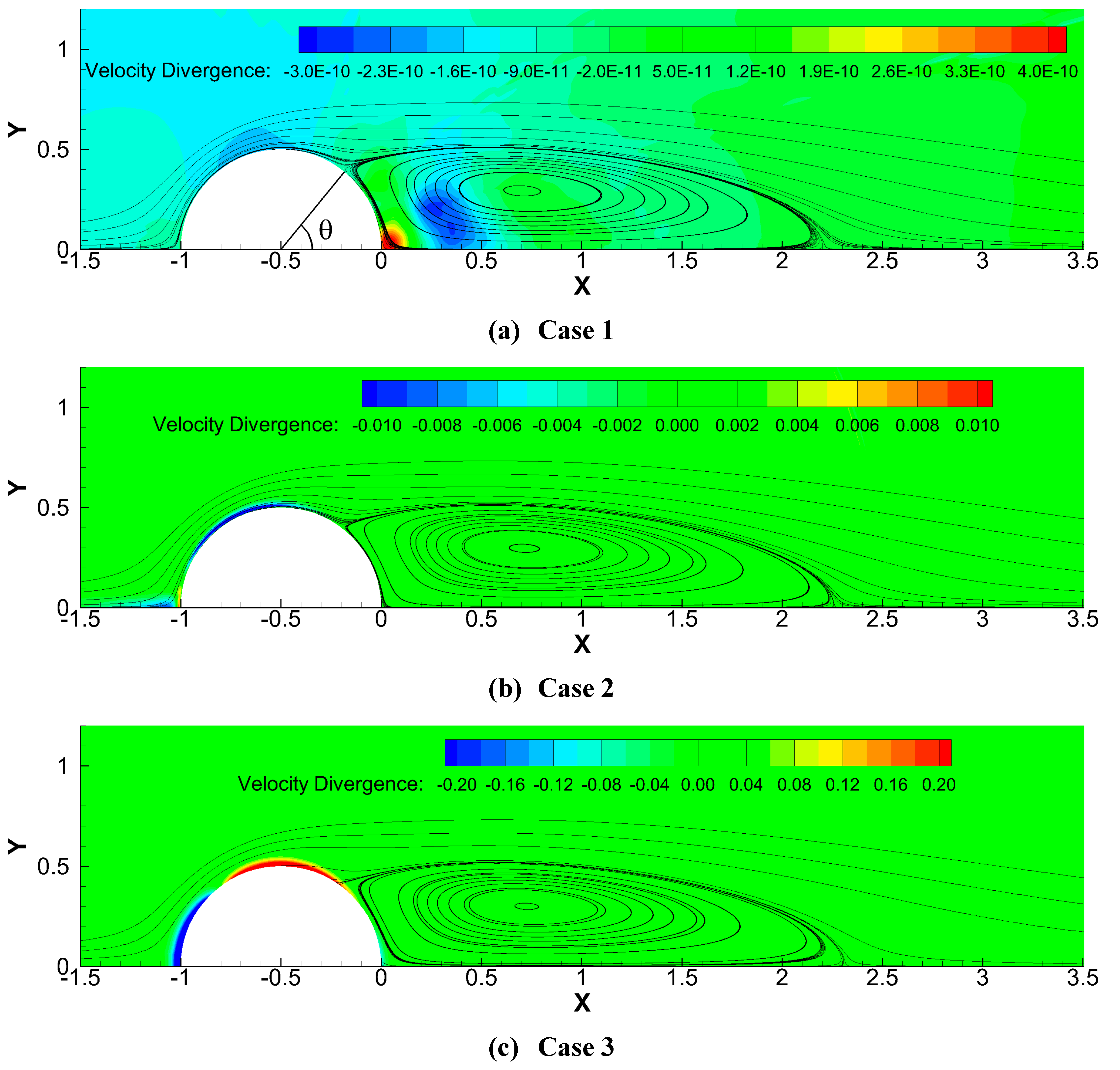
Figure 6.
Comparison of pressure and normal pressure gradient around the semi-cylinder from three simulation results.
Figure 6.
Comparison of pressure and normal pressure gradient around the semi-cylinder from three simulation results.
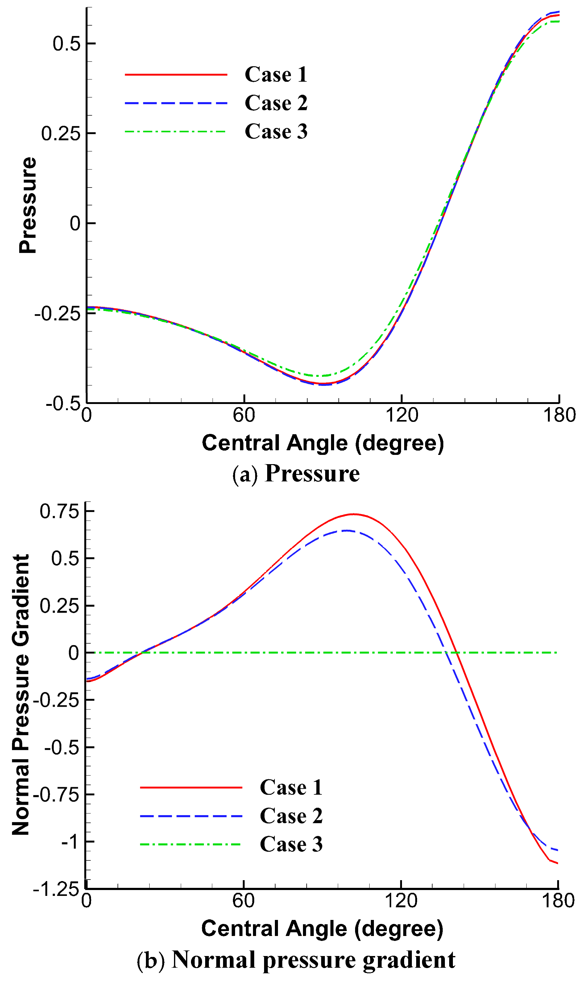

Table 1.
Test cases with Re = 100 on a 101 × 101 uniform mesh.
| Case | PPE | Neumann Boundary Condition | Max stable ∆t |
|---|---|---|---|
| 1 | Proposed PPE (7a) | Proposed BC (10) | 0.56 |
| 2 | Proposed PPE (7a) | Conventional BC (2a) | 0.09 |
| 3 | Conventional PPE (6) | Conventional BC (2a) | 0.09 |
| 4 | Conventional PPE (6) | Curl-Curl BC (2b) | 0.23 |
| 5 | Conventional PPE (6) | Homogeneous BC (1) | 0.76 |
| 6 | Conventional PPE (6) | Proposed BC (10) | 0.17 |
Table 2.
Test cases with Re = 40 on a 541 × 301 mesh.
| Case | PPE | Neumann Boundary Condition | Separation Angle |
Reattachment Distance |
|---|---|---|---|---|
| 1 | Proposed PPE (7a) | Proposed BC ((10) and (11a)) | 52.8o | 2.21 |
| 2 | Conventional PPE (6) | Conventional BC (2a) | 52.8o | 2.24 |
| 3 | Conventional PPE (6) | Homogeneous BC (1) | 52.8o | 2.31 |
| Experiments by Coutanceau and Bouard [32] | 53.5o | 2.13 | ||
Disclaimer/Publisher’s Note: The statements, opinions and data contained in all publications are solely those of the individual author(s) and contributor(s) and not of MDPI and/or the editor(s). MDPI and/or the editor(s) disclaim responsibility for any injury to people or property resulting from any ideas, methods, instructions or products referred to in the content. |
© 2025 by the authors. Licensee MDPI, Basel, Switzerland. This article is an open access article distributed under the terms and conditions of the Creative Commons Attribution (CC BY) license (http://creativecommons.org/licenses/by/4.0/).
Copyright: This open access article is published under a Creative Commons CC BY 4.0 license, which permit the free download, distribution, and reuse, provided that the author and preprint are cited in any reuse.


