Exterior 2D Div-Curl Problem for Non-Solenoidal Flows with Infinite Energy and No-Slip Boundary Condition

1. Introduction

We consider the div-curl problem in 2D exterior domain $\Omega$:

$$\begin{array}{ccc}& & \mathrm{div}\mathbf{v}\left(\mathbf{x}\right)=\rho \left(\mathbf{x}\right),\hfill \end{array}$$

(1)

$$\begin{array}{ccc}& & \mathrm{curl}\mathbf{v}\left(\mathbf{x}\right)=w\left(\mathbf{x}\right),\hfill \end{array}$$

(2)

$$\begin{array}{ccc}& & \mathbf{v}\left(\mathbf{x}\right)=0,\mathbf{x}\in \partial \Omega ,\hfill \end{array}$$

(3)

$$\begin{array}{ccc}& & \mathbf{v}\left(\mathbf{x}\right)\to {\mathbf{v}}_{\infty },\left|\mathbf{x}\right|\to \infty .\hfill \end{array}$$

(4)

Here $\mathbf{x}=(x_1,x_2)\in \Omega \subset {\mathbb{R}}^2$, $\mathbf{v}=(v_1,v_2)$ - 2D vector field, $\mathrm{curl}\mathbf{v}\left(\mathbf{x}\right)={\partial }_{x_1}{v}_2-{\partial }_{x_2}{v}_1$ is the vorticity, $\mathrm{div}\mathbf{v}\left(\mathbf{x}\right)={\partial }_{x_1}{v}_1+{\partial }_{x_2}{v}_2$ - the divergence, ${\mathbf{v}}_{\infty }\in {\mathbb{R}}^2$ - is the given fixed velocity of the flow at infinity, $\Omega ={\mathbb{R}}^2\setminus \overline{G}$ is the exterior to bounded simply connected domain G with a piecewise smooth boundary.

Quartapelle and Valz-Gris in paper [1] derived the projection conditions on the vorticity for solenoidal flows defined in bounded domains. In bounded domains for flows with finite energy this problem also was studied in [2,3,4]. In [5] author solved exterior div-curl problem in case of solenoidal flows and in [6] there was studied div-curl problem in exterior of the disk.

We will find a new orthogonality conditions for solvability of the above div-curl problem in case of non-solenoidal exterior flows. For example, for the horizontal flow ${\mathbf{v}}_{\infty }=(v_{\infty },0)$ in exterior of the disk with radius $r_0$ these conditions will have the form:

$$\begin{array}{c}\hfill {\displaystyle \frac{1}{2\pi }}{\int }_{\Omega }{\displaystyle \frac{w\left(\mathbf{x}\right)+i\rho \left(\mathbf{x}\right)}{{(x_1+i{x}_2)}^k}}d\mathbf{x}=\left\{\begin{array}{c}0,k\in \mathbb{N}\setminus \left\{1\right\},\hfill \\ i{v}_{\infty },k=1.\hfill \end{array}\right.\end{array}$$

From Stokes’ and Green’s formulas follows that in the case of the non-zero circulation or in the case of the non-zero flux at infinity we will have

$$\begin{array}{c}\hfill {\int }_{\Omega }\left(w\left(\mathbf{x}\right)+i\rho \left(\mathbf{x}\right)\right)d\mathbf{x}\ne 0.\end{array}$$

Non-zero circulation and flux at infinity generate harmonic fields with infinite kinetic energy(see [5]). In order to obtain finite $L_2$-norm $\parallel \mathbf{v}(·)-{\mathbf{v}}_{\infty }{\parallel }_{L_2}$ one should additionally impose restrictions on circulation and flux:

$$\begin{array}{cc}\hfill & \underset{R\to \infty }{lim}{\oint }_{\left|\mathbf{x}\right|=R}\mathbf{v}·d\mathbf{l}=0,\hfill \end{array}$$

(5)

$$\begin{array}{cc}\hfill & \underset{R\to \infty }{lim}{\oint }_{\left|\mathbf{x}\right|=R}(\mathbf{v},\mathbf{n})dl=0,\hfill \end{array}$$

(6)

or

$$\begin{array}{c}\hfill {\int }_{\Omega }\left(w\left(\mathbf{x}\right)+i\rho \left(\mathbf{x}\right)\right)d\mathbf{x}=0.\end{array}$$

For $L_p$-estimates of $\mathbf{v}(·)-{\mathbf{v}}_{\infty }$ with $p>2$ the above condition is not necessary.

In the paper we will use weighted space

$$\begin{array}{c}\hfill L_{2,N}(\Omega )={\{f\left(x\right):\parallel f(·)\parallel }_{L_{2,N}(\Omega )}^2={\int }_{\Omega }{\left|f\left(x\right)\right|}^2{(1+|x|}^2{)}^N\mathrm{d}x<\infty \}.\end{array}$$

Our aim is to find restrictions on w, $\rho$ for solvability of the div-curl problem (1)–(4) and to estimate its solution in $H^1$-norm as

$$\begin{array}{c}\hfill \parallel \mathbf{v}(·)-{\mathbf{v}}_{\infty }{\parallel }_{H^1(\Omega )}^2\le C\left({\parallel \rho \parallel }_{L_{2,N}(\Omega )}^2+{\parallel w\parallel }_{L_{2,N}(\Omega )}^2\right).\end{array}$$

(7)

2. Div-Cirl Problem in Exterior of the Disk

First, we study (1)–(4) in $B_{r_0}=\{\mathbf{x}\in {\mathbb{R}}^2,\left|\mathbf{x}\right|>r_0\},r_0>0$. We construct the solution of (1)–(5) in $B_{r_0}$ as Fourier series in polar coordinates r, $\phi$:

$$\begin{array}{ccc}& & \mathbf{v}(r,\phi )=\sum _{k=-\infty }^{\infty }{\mathbf{v}}_k\left(r\right)e^{ik\phi },\hfill \\ & & \rho (r,\phi )=\sum _{k=-\infty }^{\infty }{\rho }_k\left(r\right)e^{ik\phi },\hfill \\ & & w(r,\phi )=\sum _{k=-\infty }^{\infty }{w}_k\left(r\right)e^{ik\phi }.\hfill \end{array}$$

Here $\mathbf{v}(r,\phi )=(v_r,v_{\phi })$ - vector filed in polar coordinates, ${\mathbf{v}}_k\left(r\right)=(v_{r,k},v_{\phi ,k})$, ${\rho }_k$, $w_k$, - are the Fourier coefficients.

The Fourier coefficients for exterior flow ${\mathbf{v}}_{\infty }$ are given by the formulas:

$$\begin{array}{cc}\hfill & v_{r,k}^{\infty }={\displaystyle \frac{{\delta }_{\left|k\right|,1}}{2}}(v_1^{\infty }-ik{v}_2^{\infty }),\hfill \\ \hfill & v_{\phi ,k}^{\infty }={\displaystyle \frac{{\delta }_{\left|k\right|,1}}{2}}(v_2^{\infty }+ik{v}_1^{\infty }),\hfill \end{array}$$

and so we have the relation between $v_{\phi ,k}^{\infty }$ and $i{v}_{r,k}^{\infty }$:

$$\begin{array}{c}\hfill v_{\phi ,k}^{\infty }=sign\left(k\right)i{v}_{r,k}^{\infty }.\end{array}$$

Here ${\delta }_{\left|k\right|,1}=\left\{\begin{array}{c}1,\left|k\right|=1,\hfill \\ 0,\left|k\right|\ne 1.\hfill \end{array}\right.$

All the Fourier coefficients of the external flow are zero (except $k=\pm 1$). For horizontal flow ${\mathbf{v}}_{\infty }=(v_{\infty },0)$

$$\begin{array}{cc}\hfill & v_{r,k}^{\infty }={\displaystyle \frac{{\delta }_{\left|k\right|,1}}{2}}{v}_{\infty },\hfill \\ \hfill & v_{\phi ,k}^{\infty }=ik{\displaystyle \frac{{\delta }_{\left|k\right|,1}}{2}}{v}_{\infty }.\hfill \end{array}$$

Equations (1) and (2) in polar coordinates are written as:

$$\begin{array}{ccc}& & {\displaystyle \frac{1}{r}}{\displaystyle \frac{\partial }{\partial r}}\left(r{v}_{r,k}\right)+{\displaystyle \frac{ik}{r}}{v}_{\phi ,k}={\rho }_k,\hfill \\ & & {\displaystyle \frac{1}{r}}{\displaystyle \frac{\partial }{\partial r}}\left(r{v}_{\phi ,k}\right)-{\displaystyle \frac{ik}{r}}{v}_{r,k}=w_k.\hfill \end{array}$$

For non-zero k the solution of this system with condition at infinity (4) is given by the following formula:

$$\begin{array}{ccc}\hfill & & v_{r,k}={\displaystyle \frac{i{r}^{-\left|k\right|-1}}{2}}{\int }_{r_0}^r{s}^{\left|k\right|+1}\left(sign\left(k\right)w_k\left(s\right)-i{\rho }_k\left(s\right)\right)ds\hfill \\ & & +{\displaystyle \frac{i{r}^{\left|k\right|-1}}{2}}{\int }_r^{\infty }{s}^{-\left|k\right|+1}\left(sign\left(k\right)w_k\left(s\right)+i{\rho }_k\left(s\right)\right)ds+v_{r,k}^{\infty },\hfill \end{array}$$

(8)

$$\begin{array}{ccc}\hfill & & v_{\phi ,k}={\displaystyle \frac{r^{-\left|k\right|-1}}{2}}{\int }_{r_0}^r{s}^{\left|k\right|+1}\left(w_k\left(s\right)-isign\left(k\right){\rho }_k\left(s\right)\right)ds\hfill \\ & & -{\displaystyle \frac{r^{\left|k\right|-1}}{2}}{\int }_r^{\infty }{s}^{-\left|k\right|+1}\left(w_k\left(s\right)+isign\left(k\right){\rho }_k\left(s\right)\right)ds+v_{\phi ,k}^{\infty },\hfill \end{array}$$

(9)

where $sign\left(k\right)=\left\{\begin{array}{c}1,k>0\hfill \\ 0,k=0\hfill \\ -1,k<0\hfill \end{array}\right.$, ${\delta }_{\left|k\right|,1}$ - Kronecker delta.

For $k=0$ using no-slip condition (3) we have:

$$\begin{array}{cc}\hfill & v_{r,0}={\displaystyle \frac{1}{r}}{\int }_{r_0}^{r}s\rho \left(s\right)ds,\hfill \\ \hfill & v_{\phi ,0}={\displaystyle \frac{1}{r}}{\int }_{r_0}^{r}sw\left(s\right)ds.\hfill \end{array}$$

Since the conditions of zero-circulation (5) and zero-flux (6) are satisfied, then from Stokes’ and Green’s formulas

$$\begin{array}{cc}\hfill & {\int }_{r_0}^{\infty }s\rho \left(s\right)ds=0,\hfill \\ \hfill & {\int }_{r_0}^{\infty }sw\left(s\right)ds=0,\hfill \end{array}$$

and $\mathbf{v}-{\mathbf{v}}_{\infty }$ will belong to $L_2$. And Formulas (8) and (9) will be valid and for $k=0$.

These formulas have an integral representation with singular kernels:

$$\mathbf{v}\left(\mathbf{x}\right)={\displaystyle \frac{1}{2\pi }}{\int }_{B_{r_0}}{\displaystyle \frac{\mathbf{x}-\mathbf{y}}{{|\mathbf{x}-\mathbf{y}|}^2}}\rho \left(\mathbf{y}\right)d\mathbf{x}+{\displaystyle \frac{1}{2\pi }}{\int }_{B_{r_0}}{\displaystyle \frac{{(\mathbf{x}-\mathbf{y})}^{\perp }}{{|\mathbf{x}-\mathbf{y}|}^2}}w\left(\mathbf{y}\right)d\mathbf{x}+{\mathbf{v}}_{\infty },$$

(10)

where ${\mathbf{x}}^{\perp }=(-x_2,x_1)$.

The kernels in the formula above are the gradient ${\nabla }_{\mathbf{x}}$ and the skew gradient ${\nabla }_{\mathbf{x}}^{\perp }=(-{\partial }_{x_2},{\partial }_{x_1})$ of the Green function

$$\begin{array}{c}\hfill G(\mathbf{x},\mathbf{y})={\displaystyle \frac{1}{2\pi }}ln|\mathbf{x}-\mathbf{y}|.\end{array}$$

Formulas (8) and (9) with no-slip condition (3) lead to relations for $k\in \mathbb{Z}$:

$${\int }_{r_0}^{\infty }{s}^{-\left|k\right|+1}\left(w_k\left(s\right)+isign\left(k\right){\rho }_k\left(s\right)\right)ds=2ik{v}_{r,k}^{\infty }=2v_{\phi ,k}^{\infty }.$$

(11)

These relations are the orthogonality conditions

$$\begin{array}{c}\hfill {\displaystyle \frac{1}{2\pi }}{\int }_{B_{r_0}}{\displaystyle \frac{w\left(\mathbf{x}\right)+i\rho \left(\mathbf{x}\right)}{z^k}}d\mathbf{x}=\left\{\begin{array}{c}0,k\in \mathbb{N}\cup \left\{0\right\},k\ne 1,\hfill \\ 2i{v}_{r,k}^{\infty },k=1,\hfill \end{array}\right.\end{array}$$

(12)

where $z=r{e}^{i\phi }$.

The singular integrals involved in Formula (10) are the operators of Calderón-Zygmund type[7] and for $p>1$

$$\begin{array}{c}\hfill {\parallel \nabla \mathbf{v}(·)\parallel }_{L_p}\le C\left({\parallel \rho \parallel }_{L_p}+{\parallel w\parallel }_{L_p}\right).\end{array}$$

(13)

From the Hardy-Littlewood-Sobolev inequality for $1<p<2<q<\infty$, satisfying ${\displaystyle \frac{1}{q}}={\displaystyle \frac{1}{p}}-{\displaystyle \frac{1}{2}}$, the following estimate holds with some $C>0$:

$$\parallel \mathbf{v}-{\mathbf{v}}_{\infty }{\parallel }_{L_q}\le C\left({\parallel \rho \parallel }_{L_p}+{\parallel w\parallel }_{L_p}\right).$$

Theorem 1.

Suppose that the orthogonality conditions (12) are satisfied and $\rho ,w\in L_{2,N}\left(B_{r_0}\right)$ with $N>1$. Then there exists the unique solution of the div-curl problem (1)–(4) in the exterior of the disk $B_{r_0}$ and with some $C=C(r_0,N)$ the following estimate holds:

$$\begin{array}{c}\hfill \parallel \mathbf{v}(·)-{\mathbf{v}}_{\infty }{\parallel }_{H^1\left(B_{r_0}\right)}\le C\left({\parallel \rho \parallel }_{L_{2,N}\left(B_{r_0}\right)}+{\parallel w\parallel }_{L_{2,N}\left(B_{r_0}\right)}\right).\end{array}$$

(14)

Note, that from (12) with $k=0$ follows that the conditions (5) and (6) are satisfied. Existence and uniqueness follows from the explicit formulas (8) and (9).

Now we prove (14). We estimate the first term in (8) and (9) involving w for $k\ne 0$, $\left|k\right|\ne N-1$:

$$\begin{array}{cc}\hfill & \left|r^{-\left|k\right|-1}{\int }_{r_0}^r{s}^{\left|k\right|+1}{w}_k\left(s\right)ds\right|=\left|r^{-\left|k\right|-1}{\int }_{r_0}^r{\displaystyle \frac{s^{\left|k\right|+\frac{1}{2}}}{{(1+s)}^N}}{w}_k\left(s\right){(1+s)}^N\sqrt{s}ds\right|\le \hfill \\ \hfill & \left|r^{-\left|k\right|-1}{\int }_{r_0}^r{s}^{\left|k\right|+{\displaystyle \frac{1}{2}}-N}{w}_k\left(s\right){(1+s)}^N\sqrt{s}ds\right|\le \hfill \\ \hfill & r^{-\left|k\right|-1}\sqrt{{\int }_{r_0}^r{s}^{\left|2k\right|+1-2N}ds}\sqrt{{\int }_{r_0}^r{w}_k^2\left(s\right){(1+s^2)}^{N}sds}\le \hfill \\ \hfill & {\displaystyle \frac{C}{\sqrt{\left|2\right|k|-2N+2|}}}{\parallel w_k(·)\parallel }_{L_{2,N}(r_0,\infty ;r)}\left({\displaystyle \frac{1}{r^N}}+{\left({\displaystyle \frac{r_0}{r}}\right)}^{k+1}·{\displaystyle \frac{1}{r_0^N}}\right).\hfill \end{array}$$

Here $L_{2,N}(r_0,\infty ;r)$ is the weighted space of functions (with the weight ${(1+|r|}^2{)}^{N}r$) which is related to the space $L_{2,N}\left(B_{r_0}\right)$:

$$\begin{array}{c}\hfill L_{2,N}(r_0,\infty ;r)=\{f\left(r\right):\parallel f(·){\parallel }_{L_{2,N}(r_0,\infty ;r)}^2={\int }_{r_0}^{\infty }|f\left(r\right){|}^2{(1+|r|}^2{)}^{N}r\mathrm{d}r<\infty \}.\end{array}$$

Also we will use space $L_2(r_0,\infty ;r)$ related to $L_2\left(B_{r_0}\right)$:

$$\begin{array}{c}\hfill L_2(r_0,\infty ;r)=\{f\left(r\right):\parallel f(·){\parallel }_{L_2(r_0,\infty ;r)}^2={\int }_{r_0}^{\infty }|f\left(r\right){|}^{2}r\mathrm{d}r<\infty \}.\end{array}$$

Then we have $L_2$-estimate:

$$\begin{array}{cc}\hfill & {\int }_{r_0}^{\infty }{\left|r^{-\left|k\right|-1}{\int }_{r_0}^r{s}^{\left|k\right|+1}{w}_k\left(s\right)ds\right|}^{2}rdr\le \hfill \\ \hfill & {\int }_{r_0}^{\infty }{\displaystyle \frac{C^2}{\left|2\right|k|-2N+2|}}{\parallel w_k(·)\parallel }_{L_{2,N}(r_0,\infty ;r)}^2{\left({\displaystyle \frac{1}{r^N}}+{\left({\displaystyle \frac{r_0}{r}}\right)}^{k+1}·{\displaystyle \frac{1}{r_0^N}}\right)}^{2}rdr\le \hfill \\ \hfill & {\displaystyle \frac{C^2}{\left|\right|k|-N+1|}}{\parallel w_k(·)\parallel }_{L_{2,N}(r_0,\infty ;r)}^2\left({\displaystyle \frac{r_0^{-2N+2}}{2N-2}}+{\displaystyle \frac{r_0^{2-2N}}{2k}}\right).\hfill \end{array}$$

For $\left|k\right|=N-1$:

$$\begin{array}{cc}\hfill & \left|r^{-\left|k\right|-1}{\int }_{r_0}^r{s}^{\left|k\right|+1}{w}_k\left(s\right)ds\right|=\left|r^{-\left|k\right|-1}{\int }_{r_0}^r{\displaystyle \frac{s^{\left|k\right|+\frac{1}{2}}}{{(1+s)}^N}}{w}_k\left(s\right){(1+s)}^N\sqrt{s}ds\right|\le \hfill \\ \hfill & \left|r^{-\left|k\right|-1}{\int }_{r_0}^r{s}^{\left|k\right|+{\displaystyle \frac{1}{2}}-N}{w}_k\left(s\right){(1+s)}^N\sqrt{s}ds\right|\le \hfill \\ \hfill & r^{-\left|k\right|-1}\sqrt{{\int }_{r_0}^r{s}^{-1}ds}\parallel w_k{(·)\parallel }_{L_{2,N}(r_0,\infty ;r)}\le {\displaystyle \frac{\sqrt{lnr-ln{r}_0}}{r^{\left|k\right|+1}}}{\parallel w_k(·)\parallel }_{L_{2,N}(r_0,\infty ;r)}.\hfill \end{array}$$

A similar estimate is valid for $\rho$. And so, the first term in (8) and (9) for $k\ne 0$ belongs to $L_2(r_0,\infty ;r)$.

Second term in (8) and (9) we estimate in a similar way:

$$\begin{array}{cc}\hfill & \left|r^{\left|k\right|-1}{\int }_r^{\infty }{s}^{-\left|k\right|+1}{w}_k\left(s\right)ds\right|=\left|r^{\left|k\right|-1}{\int }_r^{\infty }{\displaystyle \frac{s^{-\left|k\right|+\frac{1}{2}}}{{(1+s)}^N}}{w}_k\left(s\right){(1+s)}^N\sqrt{s}ds\right|\le \hfill \\ \hfill & \left|r^{\left|k\right|-1}{\int }_r^{\infty }{s}^{-\left|k\right|+{\displaystyle \frac{1}{2}}-N}{w}_k\left(s\right){(1+s)}^N\sqrt{s}ds\right|\le \hfill \\ \hfill & r^{\left|k\right|-1}\sqrt{{\int }_r^{\infty }{s}^{-\left|2k\right|+1-2N}ds}\sqrt{{\int }_r^{\infty }{w}_k^2\left(s\right){(1+s^2)}^{N}sds}\le \hfill \\ \hfill & {\displaystyle \frac{1}{r^N\sqrt{\left|2\right|k|+2N-2|}}}{\parallel w_k(·)\parallel }_{L_{2,N}(r_0,\infty ;r)}.\hfill \end{array}$$

So, for $k\ne 0$ it also belongs to $L_2(r_0,\infty ;r)$. Lets study the case $k=0$. We have

$$\begin{array}{c}\hfill v_{\phi ,0}={\displaystyle \frac{1}{r}}{\int }_{r_0}^{r}s{w}_0\left(s\right)ds=-{\displaystyle \frac{1}{r}}{\int }_r^{\infty }s{w}_0\left(s\right)ds,\end{array}$$

and

$$\begin{array}{cc}\hfill & |v_{\phi ,0}|=\left|{\displaystyle \frac{1}{r}}{\int }_r^{\infty }s{w}_0\left(s\right)ds\right|\le \hfill \\ \hfill & \left|r^{-1}{\int }_r^{\infty }{s}^{{\displaystyle \frac{1}{2}}-N}{w}_0\left(s\right){(1+s)}^N\sqrt{s}ds\right|\le \hfill \\ \hfill & r^{-1}\sqrt{{\int }_r^{\infty }{s}^{1-2N}ds}\sqrt{{\int }_r^{\infty }{w}_0^2\left(s\right){(1+s^2)}^{N}sds}\le \hfill \\ \hfill & {\displaystyle \frac{1}{r^N\sqrt{2N-2}}}{\parallel w_0(·)\parallel }_{L_{2,N}(r_0,\infty ;r)}.\hfill \end{array}$$

In a similar way

$$\begin{array}{c}\hfill |v_{r,0}|\le {\displaystyle \frac{1}{r^N\sqrt{2N-2}}}{\parallel {\rho }_0(·)\parallel }_{L_{2,N}(r_0,\infty ;r)}.\end{array}$$

So, $v_{r,0}$, $v_{\phi ,0}$ will belong to $L_2(r_0,\infty ;r)$. Then, summing by k, and using Parseval’s equality for Fourier series, we obtain the inequality with some $C=C(r_0,N)$:

$$\begin{array}{c}\hfill \parallel \mathbf{v}(·)-{\mathbf{v}}_{\infty }{\parallel }_{L_2\left(B_{r_0}\right)}\le C\left({\parallel \rho \parallel }_{L_{2,N}\left(B_{r_0}\right)}+{\parallel w\parallel }_{L_{2,N}\left(B_{r_0}\right)}\right).\end{array}$$

Finally, in virtue of the inequality (13) we obtain the required estimate (14).

3. Div-cirl Problem in Exterior Domain

For further consideration we need some additional requirements on $\Omega$. Suppose the there exists a Riemann mapping $\Phi$ from $\Omega$ into $B_{r_0}$ such that

$$\begin{array}{c}\hfill \Phi \left(p\right)=p+O\left({\displaystyle \frac{1}{p}}\right),\end{array}$$

where $p=y_1+i{y}_2\in \mathbb{C}$.

And also suppose that for $z=x_1+i{x}_2\in \mathbb{C}$ there exists the inverse transform ${\Phi }^{-1}\left(z\right):B_{r_0}\to \Omega$, which satisfies

$$\begin{array}{c}\hfill {\Phi }^{-1}\left(z\right)=z+O\left({\displaystyle \frac{1}{z}}\right),\end{array}$$

(15)

and

$$\begin{array}{c}\hfill {\left({\Phi }^{-1}\right)}^{\prime }\left(z\right)=1+O\left({\displaystyle \frac{1}{z^2}}\right).\end{array}$$

(16)

We change the variables $\mathbf{y}=(y_1,y_2)\in \Omega$ onto $\mathbf{x}=(x_1,x_2)\in B_{r_0}$ in the system (1) and (2). Vector field $\mathbf{v}\left(p\right)$ in $\Omega$ with $p=y_1+i{y}_2$ defines the vector field $\widehat{\mathbf{v}}\left(\mathbf{x}\right)$ in $B_{r_0}$:

$$\begin{array}{c}\hfill \mathbf{v}\left(\mathbf{y}\right)=D{\Phi }^t\widehat{\mathbf{v}}\left(\mathbf{x}\left(\mathbf{y}\right)\right),\end{array}$$

where $D{\Phi }^t$ is the transpose matrix to Jacobian matrix $D\Phi$

$$\begin{array}{c}\hfill D\Phi =\left(\begin{array}{ccc}& Re{\Phi }_{x_1}^{\prime }& Re{\Phi }_{x_2}^{\prime }\\ & Im{\Phi }_{x_1}^{\prime }& Im{\Phi }_{x_2}^{\prime }\end{array}\right)=\left(\begin{array}{ccc}& Re{\Phi }_{x_1}^{\prime }& -Im{\Phi }_{x_1}^{\prime }\\ & Im{\Phi }_{x_1}^{\prime }& Re{\Phi }_{x_1}^{\prime }\end{array}\right).\end{array}$$

Then

$$\begin{array}{cc}\hfill & \widehat{\mathbf{v}}\left(\mathbf{x}\right)={D{\Phi }^{-1}}^t\mathbf{v}\left({\Phi }^{-1}\left(\mathbf{x}\right)\right)=\hfill \\ & {D{\Phi }^{-1}}^t\mathbf{v}(Re{\Phi }^{-1}(x_1+i{x}_2),Im{\Phi }^{-1}(x_1+i{x}_2))\hfill \end{array}$$

(17)

is the vector field in $B_{r_0}$. And $\widehat{\rho }\left(\mathbf{x}\right)=\rho (\Phi \left(\mathbf{x}\right))$, $\widehat{w}\left(\mathbf{x}\right)=w(\Phi \left(\mathbf{x}\right))$ are the divergence and vorticity functions in $B_{r_0}$ correspondingly.

From the Cauchy-Riemann relations

$$\begin{array}{cc}\hfill & {\displaystyle \frac{\partial x_1}{\partial y_1}}={\displaystyle \frac{\partial x_2}{\partial y_2}},\hfill \\ \hfill & {\displaystyle \frac{\partial x_2}{\partial y_1}}=-{\displaystyle \frac{\partial x_1}{\partial y_2}}\hfill \end{array}$$

we will have

$$\begin{array}{c}\hfill {div}_{\mathbf{y}}\mathbf{v}\left(\mathbf{y}\right)={\displaystyle \frac{\partial v_1}{\partial y_1}}+{\displaystyle \frac{\partial v_2}{\partial y_2}}={\displaystyle \frac{\partial v_1}{\partial x_1}}{\displaystyle \frac{\partial x_1}{\partial y_1}}+{\displaystyle \frac{\partial v_1}{\partial x_2}}{\displaystyle \frac{\partial x_2}{\partial y_1}}+{\displaystyle \frac{\partial v_2}{\partial x_1}}{\displaystyle \frac{\partial x_1}{\partial y_2}}+{\displaystyle \frac{\partial v_2}{\partial x_2}}{\displaystyle \frac{\partial x_2}{\partial y_2}}\\ \hfill ={\displaystyle \frac{\partial v_1}{\partial x_1}}{\displaystyle \frac{\partial x_1}{\partial y_1}}+{\displaystyle \frac{\partial v_1}{\partial x_2}}{\displaystyle \frac{\partial x_2}{\partial y_1}}+{\displaystyle \frac{\partial v_2}{\partial x_1}}{\displaystyle \frac{\partial x_1}{\partial y_2}}+{\displaystyle \frac{\partial v_2}{\partial x_2}}{\displaystyle \frac{\partial x_2}{\partial y_2}}={\displaystyle \frac{\partial x_1}{\partial y_1}}\left({\displaystyle \frac{\partial v_1}{\partial x_1}}+{\displaystyle \frac{\partial v_2}{\partial x_2}}\right)\\ \hfill -{\displaystyle \frac{\partial x_2}{\partial y_1}}\left({\displaystyle \frac{\partial v_2}{\partial x_1}}-{\displaystyle \frac{\partial v_1}{\partial x_2}}\right)={\displaystyle \frac{\partial x_1}{\partial y_1}}{div}_{\mathbf{x}}\mathbf{v}\left(\mathbf{x}\right)-{\displaystyle \frac{\partial x_2}{\partial y_1}}{curl}_{\mathbf{x}}\mathbf{v}\left(\mathbf{x}\right),\end{array}$$

and

$$\begin{array}{c}\hfill {curl}_{\mathbf{y}}\mathbf{v}\left(\mathbf{y}\right)={\displaystyle \frac{\partial v_2}{\partial y_1}}-{\displaystyle \frac{\partial v_1}{\partial y_2}}={\displaystyle \frac{\partial v_2}{\partial x_1}}{\displaystyle \frac{\partial x_1}{\partial y_1}}+{\displaystyle \frac{\partial v_2}{\partial x_2}}{\displaystyle \frac{\partial x_2}{\partial y_1}}-{\displaystyle \frac{\partial v_1}{\partial x_1}}{\displaystyle \frac{\partial x_1}{\partial y_2}}-{\displaystyle \frac{\partial v_1}{\partial x_2}}{\displaystyle \frac{\partial x_2}{\partial y_2}}\\ \hfill ={\displaystyle \frac{\partial x_1}{\partial y_1}}{curl}_{\mathbf{x}}\mathbf{v}\left(\mathbf{x}\right)+{\displaystyle \frac{\partial x_2}{\partial y_1}}{div}_{\mathbf{x}}\mathbf{v}\left(\mathbf{x}\right).\end{array}$$

Finally, the system (1) and (2) goes to

$$\begin{array}{cc}\hfill & {\displaystyle \frac{\partial x_1}{\partial y_1}}{div}_{\mathbf{x}}\mathbf{v}\left(\mathbf{x}\right)-{\displaystyle \frac{\partial x_2}{\partial y_1}}{curl}_{\mathbf{x}}\mathbf{v}\left(\mathbf{x}\right)=\widehat{\rho }\left(\mathbf{x}\right),\hfill \\ \hfill & {\displaystyle \frac{\partial x_2}{\partial y_1}}{div}_{\mathbf{x}}\mathbf{v}\left(\mathbf{x}\right)+{\displaystyle \frac{\partial x_1}{\partial y_1}}{curl}_{\mathbf{x}}\mathbf{v}\left(\mathbf{x}\right)=\widehat{w}\left(\mathbf{x}\right).\hfill \end{array}$$

Then

$$\begin{array}{c}\hfill {div}_{\mathbf{x}}\mathbf{v}\left(\mathbf{x}\right)={\displaystyle \frac{\frac{\partial x_2}{\partial y_2}}{{\left(\frac{\partial x_1}{\partial y_1}\right)}^2+{\left(\frac{\partial x_1}{\partial y_2}\right)}^2}}\widehat{\rho }\left(\mathbf{x}\right)+{\displaystyle \frac{\frac{\partial x_2}{\partial y_1}}{{\left(\frac{\partial x_1}{\partial y_1}\right)}^2+{\left(\frac{\partial x_1}{\partial y_2}\right)}^2}}\widehat{w}\left(\mathbf{x}\right),\\ \hfill {curl}_{\mathbf{x}}\mathbf{v}\left(\mathbf{x}\right)=-{\displaystyle \frac{\frac{\partial x_2}{\partial y_1}}{{\left(\frac{\partial x_1}{\partial y_1}\right)}^2+{\left(\frac{\partial x_1}{\partial y_2}\right)}^2}}\widehat{\rho }\left(\mathbf{x}\right)+{\displaystyle \frac{\frac{\partial x_1}{\partial y_1}}{{\left(\frac{\partial x_1}{\partial y_1}\right)}^2+{\left(\frac{\partial x_1}{\partial y_2}\right)}^2}}\widehat{w}\left(\mathbf{x}\right).\end{array}$$

Using the representation of the complex derivative ${\Phi }^{\prime }\left(p\right)$:

$$\begin{array}{c}\hfill {\Phi }^{\prime }\left(p\right)={\displaystyle \frac{\partial x_1}{\partial y_1}}+i{\displaystyle \frac{\partial x_2}{\partial y_1}}={\displaystyle \frac{\partial x_2}{\partial y_2}}-i{\displaystyle \frac{\partial x_1}{\partial y_2}}\end{array}$$

we will have

$$curl{\mathbf{v}}_{\mathbf{x}}+idiv{\mathbf{v}}_{\mathbf{x}}={\displaystyle \frac{{\Phi }^{\prime }\left(p\right)}{|{\Phi }^{\prime }{\left(p\right)|}^2}}\widehat{w}+i\overline{{\displaystyle \frac{{\Phi }^{\prime }\left(p\right)}{|{\Phi }^{\prime }{\left(p\right)|}^2}}}\widehat{\rho }.$$

Now we calculate the divergence of the field $\widehat{\mathbf{v}}={D{\Phi }^{-1}}^t\mathbf{v}\left({\Phi }^{-1}\left(\mathbf{x}\right)\right)$. Using Jacobian matrix

$$\begin{array}{c}\hfill D{\Phi }^{-1}=\left(\begin{array}{ccc}& {\displaystyle \frac{\partial y_1}{\partial x_1}}& -{\displaystyle \frac{\partial y_2}{\partial x_1}}\\ & {\displaystyle \frac{\partial y_2}{\partial x_1}}& {\displaystyle \frac{\partial y_1}{\partial x_1}}\end{array}\right)={\displaystyle \frac{1}{|{\Phi }^{\prime }{|}^2}}\left(\begin{array}{ccc}& {\displaystyle \frac{\partial x_1}{\partial y_1}}& {\displaystyle \frac{\partial x_2}{\partial y_1}}\\ & -{\displaystyle \frac{\partial x_2}{\partial y_1}}& {\displaystyle \frac{\partial x_1}{\partial y_1}}\end{array}\right)\end{array}$$

and its transpose

$$\begin{array}{c}\hfill {D{\Phi }^{-1}}^t=\left(\begin{array}{ccc}& {\displaystyle \frac{\partial y_1}{\partial x_1}}& {\displaystyle \frac{\partial y_2}{\partial x_1}}\\ & -{\displaystyle \frac{\partial y_2}{\partial x_1}}& {\displaystyle \frac{\partial y_1}{\partial x_1}}\end{array}\right)={\displaystyle \frac{1}{|{\Phi }^{\prime }{|}^2}}\left(\begin{array}{ccc}& {\displaystyle \frac{\partial x_1}{\partial y_1}}& -{\displaystyle \frac{\partial x_2}{\partial y_1}}\\ & {\displaystyle \frac{\partial x_2}{\partial y_1}}& {\displaystyle \frac{\partial x_1}{\partial y_1}}\end{array}\right)\end{array}$$

we will have

$$\begin{array}{cc}\hfill & {div}_{\mathbf{x}}\widehat{\mathbf{v}}\left(\mathbf{x}\right)={\displaystyle \frac{\partial y_1}{\partial x_1}}{div}_{\mathbf{x}}\mathbf{v}+{\displaystyle \frac{\partial y_2}{\partial x_1}}{curl}_{\mathbf{x}}\mathbf{v}=\hfill \\ \hfill & {\displaystyle \frac{1}{|{\Phi }^{\prime }{|}^2}}\left({\displaystyle \frac{\partial y_1}{\partial x_1}}{\displaystyle \frac{\partial x_2}{\partial y_1}}+{\displaystyle \frac{\partial y_2}{\partial x_1}}{\displaystyle \frac{\partial x_1}{\partial y_1}}\right)\widehat{w}+{\displaystyle \frac{1}{|{\Phi }^{\prime }{|}^2}}\left({\displaystyle \frac{\partial y_1}{\partial x_1}}{\displaystyle \frac{\partial x_2}{\partial y_2}}+{\displaystyle \frac{\partial y_2}{\partial x_1}}{\displaystyle \frac{\partial x_2}{\partial y_1}}\right)\widehat{\rho }=\hfill \\ \hfill & \left({\left({\displaystyle \frac{\partial y_1}{\partial x_1}}\right)}^2+{\left({\displaystyle \frac{\partial y_2}{\partial x_1}}\right)}^2\right)\widehat{\rho }={\left|{{\Phi }^{-1}}^{\prime }\right|}^2\widehat{\rho }\hfill \end{array}$$

and

$$\begin{array}{cc}\hfill & {curl}_{\mathbf{x}}\widehat{\mathbf{v}}\left(\mathbf{x}\right)={\displaystyle \frac{\partial y_1}{\partial x_1}}{curl}_{\mathbf{x}}\mathbf{v}-{\displaystyle \frac{\partial y_2}{\partial x_1}}{div}_{\mathbf{x}}\mathbf{v}=\hfill \\ \hfill & {\displaystyle \frac{1}{|{\Phi }^{\prime }{|}^2}}\left({\displaystyle \frac{\partial y_1}{\partial x_1}}{\displaystyle \frac{\partial x_1}{\partial y_1}}-{\displaystyle \frac{\partial y_2}{\partial x_1}}{\displaystyle \frac{\partial x_2}{\partial y_1}}\right)\widehat{w}+{\displaystyle \frac{1}{|{\Phi }^{\prime }{|}^2}}\left(-{\displaystyle \frac{\partial y_1}{\partial x_1}}{\displaystyle \frac{\partial x_2}{\partial y_1}}-{\displaystyle \frac{\partial y_2}{\partial x_1}}{\displaystyle \frac{\partial x_2}{\partial y_2}}\right)\widehat{\rho }=\hfill \\ \hfill & \left({\left({\displaystyle \frac{\partial y_1}{\partial x_1}}\right)}^2+{\left({\displaystyle \frac{\partial y_2}{\partial x_1}}\right)}^2\right)\widehat{w}={\left|{{\Phi }^{-1}}^{\prime }\right|}^2\widehat{w}.\hfill \end{array}$$

Then the system (1)–(4) transfers to new one, defined in $B_{r_0}$:

$$\begin{array}{ccc}& & div\widehat{\mathbf{v}}\left(\mathbf{x}\right)={\left|{{\Phi }^{-1}}^{\prime }\right|}^2\widehat{\rho }\left(\mathbf{x}\right),\hfill \end{array}$$

(18)

$$\begin{array}{ccc}& & curl\widehat{\mathbf{v}}\left(\mathbf{x}\right)={\left|{{\Phi }^{-1}}^{\prime }\right|}^2\widehat{w}\left(\mathbf{x}\right),\hfill \end{array}$$

(19)

$$\begin{array}{ccc}& & \widehat{\mathbf{v}}\left(\mathbf{x}\right)=0,\left|\mathbf{x}\right|=r_0,\hfill \end{array}$$

(20)

$$\begin{array}{ccc}& & \widehat{\mathbf{v}}\left(\mathbf{x}\right)\to {\mathbf{v}}_{\infty },\left|\mathbf{x}\right|\to \infty .\hfill \end{array}$$

(21)

Denote

$$\begin{array}{c}\hfill q_k\left(r\right)=\left[\right|{{\Phi }^{-1}}^{\prime }\left(z\right){{|}^2\widehat{w}\left(\mathbf{x}\right)]}_k,\\ \hfill r_k\left(r\right)=\left[\right|{{\Phi }^{-1}}^{\prime }\left(z\right){{|}^2\widehat{\rho }\left(\mathbf{x}\right)]}_k,\end{array}$$

where ${[·]}_k$ means the k-th Fourier coefficient and $z=r{e}^{i\phi }=x_1+i{x}_2$.

Rewrite (18) and (19) in polar coordinates using Fourier coefficients ${\widehat{v}}_{r,k}$, ${\widehat{v}}_{\phi ,k}$:

$$\begin{array}{ccc}& & {\displaystyle \frac{1}{r}}{\displaystyle \frac{\partial }{\partial r}}\left(r{\widehat{v}}_{r,k}\right)+{\displaystyle \frac{ik}{r}}{\widehat{v}}_{\phi ,k}=r_k\left(r\right),\hfill \\ & & {\displaystyle \frac{1}{r}}{\displaystyle \frac{\partial }{\partial r}}\left(r{\widehat{v}}_{\phi ,k}\right)-{\displaystyle \frac{ik}{r}}{\widehat{v}}_{r,k}=q_k\left(r\right).\hfill \end{array}$$

From (5) and (6), Stokes and divergence formulas we have:

$$\begin{array}{c}\hfill \underset{R\to \infty }{lim}{\oint }_{\left|\mathbf{x}\right|=R}\widehat{\mathbf{v}}\left(\mathbf{x}\right)·d\mathbf{l}={\int }_{B_{r_0}}\widehat{w}\left(\mathbf{x}\right)d\mathbf{x}={\int }_{B_{r_0}}{\displaystyle \frac{\widehat{w}\left(\mathbf{x}\right)}{|{\Phi }^{\prime }{|}^2}}d\mathbf{x}=\\ \hfill 2\pi {\int }_{r_0}^{\infty }{\left[{\displaystyle \frac{\widehat{w}\left(\mathbf{x}\right)}{|{\Phi }^{\prime }{|}^2}}\right]}_{k=0}sds=0\\ \hfill \underset{R\to \infty }{lim}{\oint }_{\left|\mathbf{x}\right|=R}(\widehat{\mathbf{v}}\left(\mathbf{x}\right),\mathbf{n})dl={\int }_{B_{r_0}}\widehat{\rho }\left(\mathbf{x}\right)d\mathbf{x}={\int }_{B_{r_0}}{\displaystyle \frac{\widehat{\rho }\left(\mathbf{x}\right)}{|{\Phi }^{\prime }{|}^2}}d\mathbf{x}=\\ \hfill 2\pi {\int }_{r_0}^{\infty }{\left[{\displaystyle \frac{\widehat{\rho }\left(\mathbf{x}\right)}{|{\Phi }^{\prime }{|}^2}}\right]}_{k=0}sds=0.\end{array}$$

The solution of the system (18)–(21) is given by

$$\begin{array}{ccc}\hfill & & {\widehat{v}}_{r,k}={\displaystyle \frac{i{r}^{-\left|k\right|-1}}{2}}{\int }_{r_0}^r{s}^{\left|k\right|+1}(sign\left(k\right)q_k-i{r}_k)ds\hfill \\ & & +{\displaystyle \frac{i{r}^{\left|k\right|-1}}{2}}{\int }_r^{\infty }{s}^{-\left|k\right|+1}(sign\left(k\right)q_k+i{r}_k)ds+v_{r,k}^{\infty },\hfill \end{array}$$

(22)

$$\begin{array}{ccc}\hfill & & {\widehat{v}}_{\phi ,k}={\displaystyle \frac{r^{-\left|k\right|-1}}{2}}{\int }_{r_0}^r{s}^{\left|k\right|+1}(q_k-isign\left(k\right)r_k)ds\hfill \\ & & -{\displaystyle \frac{r^{\left|k\right|-1}}{2}}{\int }_r^{\infty }{s}^{-\left|k\right|+1}(q_k+isign\left(k\right)r_k)ds+v_{\phi ,k}^{\infty }.\hfill \end{array}$$

(23)

Formulas (22) and (23) with no-slip condition (20) lead to relations ($k\in \mathbb{Z}$):

$${\int }_{r_0}^{\infty }{s}^{-\left|k\right|+1}(q_k+i{r}_k)ds=2ik{v}_{r,k}^{\infty }=2v_{\phi ,k}^{\infty },$$

or

$${\displaystyle \frac{1}{2\pi }}{\int }_{B_{r_0}}{\displaystyle \frac{\widehat{w}\left({\Phi }^{-1}\left(\mathbf{x}\right)\right)+i\widehat{\rho }\left({\Phi }^{-1}\left(\mathbf{x}\right)\right)}{z^k}}{\left|{{\Phi }^{-1}}^{\prime }\left(\mathbf{x}\right)\right|}^{2}d\mathbf{x}=2ik{v}_{r,k}^{\infty }=2v_{\phi ,k}^{\infty }$$

for $k\in \mathbb{N}\cup \left\{0\right\}$.

Finally, these moment relations in $\Omega$ will take the form

$$\begin{array}{c}\hfill {\displaystyle \frac{1}{2\pi }}{\int }_{\Omega }{\displaystyle \frac{w\left(\mathbf{x}\right)+i\rho \left(\mathbf{x}\right)}{\Phi {\left(z\right)}^k}}d\mathbf{x}=2ik{v}_{r,k}^{\infty }=2v_{\phi ,k}^{\infty },k\in \mathbb{N}\cup \left\{0\right\}.\end{array}$$

(24)

For horizontal flow ${\mathbf{v}}_{\infty }=(v_{\infty },0)$ it will be the relations

$$\begin{array}{c}\hfill {\displaystyle \frac{1}{2\pi }}{\int }_{\Omega }{\displaystyle \frac{w\left(\mathbf{x}\right)+i\rho \left(\mathbf{x}\right)}{\Phi {\left(z\right)}^k}}d\mathbf{x}=\left\{\begin{array}{c}0,k\in \mathbb{N}\cup \left\{0\right\},k\ne 1,\hfill \\ i{v}_{\infty },k=1.\hfill \end{array}\right.\end{array}$$

Formulas (22) and (23) have an integral representation

$$\begin{array}{c}\hfill \widehat{\mathbf{v}}\left(\mathbf{x}\right)={\displaystyle \frac{1}{2\pi }}{\int }_{B_{r_0}}{\displaystyle \frac{{(\mathbf{x}-\mathbf{y})}^{\perp }}{{|\mathbf{x}-\mathbf{y}|}^2}}{\left|{{\Phi }^{-1}}^{\prime }\left(\mathbf{y}\right)\right|}^2\widehat{w}\left(\mathbf{y}\right)d\mathbf{y}+\\ \hfill {\displaystyle \frac{1}{2\pi }}{\int }_{B_{r_0}}{\displaystyle \frac{\mathbf{x}-\mathbf{y}}{{|\mathbf{x}-\mathbf{y}|}^2}}{\left|{{\Phi }^{-1}}^{\prime }\left(\mathbf{y}\right)\right|}^2\widehat{\rho }\left(\mathbf{y}\right)d\mathbf{y}+{\mathbf{v}}_{\infty }.\end{array}$$

In $\Omega$ this formula takes the form

$$\begin{array}{c}\hfill \mathbf{v}\left(\mathbf{x}\right)={\displaystyle \frac{1}{2\pi }}D{\Phi }^t\left(\mathbf{x}\right){\int }_{\Omega }{\displaystyle \frac{{(\Phi \left(\mathbf{x}\right)-\Phi \left(\mathbf{y}\right))}^{\perp }}{{|\Phi \left(\mathbf{x}\right)-\Phi \left(\mathbf{y}\right)|}^2}}w\left(\mathbf{y}\right)d\mathbf{y}+\\ \hfill {\displaystyle \frac{1}{2\pi }}D{\Phi }^t\left(\mathbf{x}\right){\int }_{\Omega }{\displaystyle \frac{\Phi \left(\mathbf{x}\right)-\Phi \left(\mathbf{y}\right)}{{|\Phi \left(\mathbf{x}\right)-\Phi \left(\mathbf{y}\right)|}^2}}\rho \left(\mathbf{y}\right)d\mathbf{y}+{\mathbf{v}}_{\infty }.\end{array}$$

(25)

The kernels of integrals involved in above formula are the gradient and the skew gradient of the Green’s function:

$$\begin{array}{c}\hfill G(\mathbf{x},\mathbf{y})={\displaystyle \frac{1}{2\pi }}ln|\Phi \left(\mathbf{x}\right)-\Phi \left(\mathbf{y}\right)|.\end{array}$$

4. Uniqueness Solvability of the div-curl Problem

Theorem 2.

Let Ω be the exterior domain with a piecewise smooth boundary such that there exists a Riemann mapping from Ω into $B_{r_0}$ satisfying (15) and (16), $\rho ,w\in L_{2,N}(\Omega )$ with $N>1$, and the moment relations (24) are satisfied. Then there exists the unique solution $\mathbf{v}$ of the problem (1)–(4), and the estimate (7) holds.

Uniqueness follows from the Hodge theory, since the no-slip condition fixes circulation and flux around a solid and in that case there is no one nontrivial harmonic form. Existence follows from the explicit formula for the solution (22) and (23), or its integral representation (25).

From (24) we have

$$\begin{array}{c}\hfill {\int }_{B_{r_0}}w\left({\Phi }^{-1}\left(\mathbf{x}\right)\right){\left|{{\Phi }^{-1}}^{\prime }\left(\mathbf{x}\right)\right|}^{2}d\mathbf{x}=0,\\ \hfill {\int }_{B_{r_0}}\rho \left({\Phi }^{-1}\left(\mathbf{x}\right)\right){\left|{{\Phi }^{-1}}^{\prime }\left(\mathbf{x}\right)\right|}^{2}d\mathbf{x}=0.\end{array}$$

Then from Theorem 1 using (16) with some $C_1$, $C_2$ holds:

$$\begin{array}{c}\hfill \parallel \widehat{\mathbf{v}}(·)-{\mathbf{v}}_{\infty }{\parallel }_{H^1\left(B_{r_0}\right)}\le C_1{∥\rho \left({\Phi }^{-1}(·)\right)|{{\Phi }^{-1}}^{\prime }{(·)|}^2+w\left({\Phi }^{-1}(·)\right){\left|{{\Phi }^{-1}}^{\prime }(·)\right|}^2∥}_{L_{2,N}\left(B_{r_0}\right)}\\ \hfill \le C_2\left({\parallel w(·)\parallel }_{L_{2,N}(\Omega )}+{\parallel \rho (·)\parallel }_{L_{2,N}(\Omega )}\right).\end{array}$$

Finally, using the inequality with some $C_3$

$$\begin{array}{c}\hfill \parallel \mathbf{v}(·)-{\mathbf{v}}_{\infty }{\parallel }_{H^1(\Omega )}\le C_3{\parallel \widehat{\mathbf{v}}(·)-{\mathbf{v}}_{\infty }\parallel }_{H^1\left(B_{r_0}\right)}\end{array}$$

we obtain the estimate (7). The Theorem is proved.

5. Numerical Results

Here we will present the method for solving the exterior div-curl problem

$$\begin{array}{ccc}& & \mathrm{div}\mathbf{v}\left(\mathbf{x}\right)=0,\hfill \end{array}$$

(26)

$$\begin{array}{ccc}& & \mathrm{curl}\mathbf{v}\left(\mathbf{x}\right)=w\left(\mathbf{x}\right),\hfill \end{array}$$

(27)

$$\begin{array}{ccc}& & \mathbf{v}\left(\mathbf{x}\right)=0,\mathbf{x}\in \partial \Omega ,\hfill \end{array}$$

(28)

$$\begin{array}{ccc}& & \mathbf{v}\left(\mathbf{x}\right)\to (v_{\infty },0),\left|\mathbf{x}\right|\to \infty ,\hfill \end{array}$$

(29)

which can be realized numerically for solenoidal flows with no-slip condition on the solid and horizontal flow at infinity $(v_{\infty },0)$. For these flows since the no-slip condition (28) is fullfiled, then there exists a stream function $\psi$, such that

$$\mathbf{v}={\nabla }^{\perp }\psi ,$$

where ${\nabla }_{\mathbf{x}}^{\perp }=(-{\partial }_{x_2},{\partial }_{x_1})$.

The condition (28) is a particular case of slip interaction between solid and fluid, which is expressed by the formula:

$$\begin{array}{c}\hfill (\mathbf{v},\mathbf{n})=0,\mathbf{x}\in \partial \Omega .\end{array}$$

(30)

In terms of stream function it can be rewritten as

$$\begin{array}{c}\hfill \psi \left(\mathbf{x}\right)\equiv const,\mathbf{x}\in \partial \Omega .\end{array}$$

(31)

Also no-slip condition leads to Neumann boundary ones:

$$\begin{array}{c}\hfill {\displaystyle \frac{\partial \psi \left(\mathbf{x}\right)}{\partial \mathbf{n}}}=0,\mathbf{x}\in \partial \Omega .\end{array}$$

(32)

At infinity horizontal flow $(v_{\infty },0)$ transfers to boundary constraint on $\psi$:

$$\begin{array}{c}\hfill \psi \left(\mathbf{x}\right)\to -v_{\infty }·x_2,\left|\mathbf{x}\right|\to \infty .\end{array}$$

(33)

The Equation (27) goes to Poisson equation under curl operator:

$$\begin{array}{c}\hfill \Delta \psi =curl\mathbf{v}.\end{array}$$

(34)

But the exterior Poisson problem with boundary condition (31)–(33) is overdetermined and incorrect. From (28) follows zero-circulation condition around boundary

$$\begin{array}{c}\hfill {\oint }_{\partial \Omega }\mathbf{v}·d\mathbf{l}=0.\end{array}$$

(35)

This condition combined with slip constraint (30) guarantees the correctness of the exterior div-curl problem (26), (27) and (29). And so (31), (33) and (35) guarantee the correctness of the exterior Poisson problem (34) which can be solved numerically by means of finite elements method (FEM). Conditions (31) and (35) generate N boundary relations, where N is the amount of boundary nodes in a triangulated domain. Unbounded domain is restricted by rectangular domain where we set the condition on infinity (33). This condition also generates relations by the number of nodes in rectangular domain. So, FEM becomes a closed numerical method for the system (31), (33), (34) and (35).

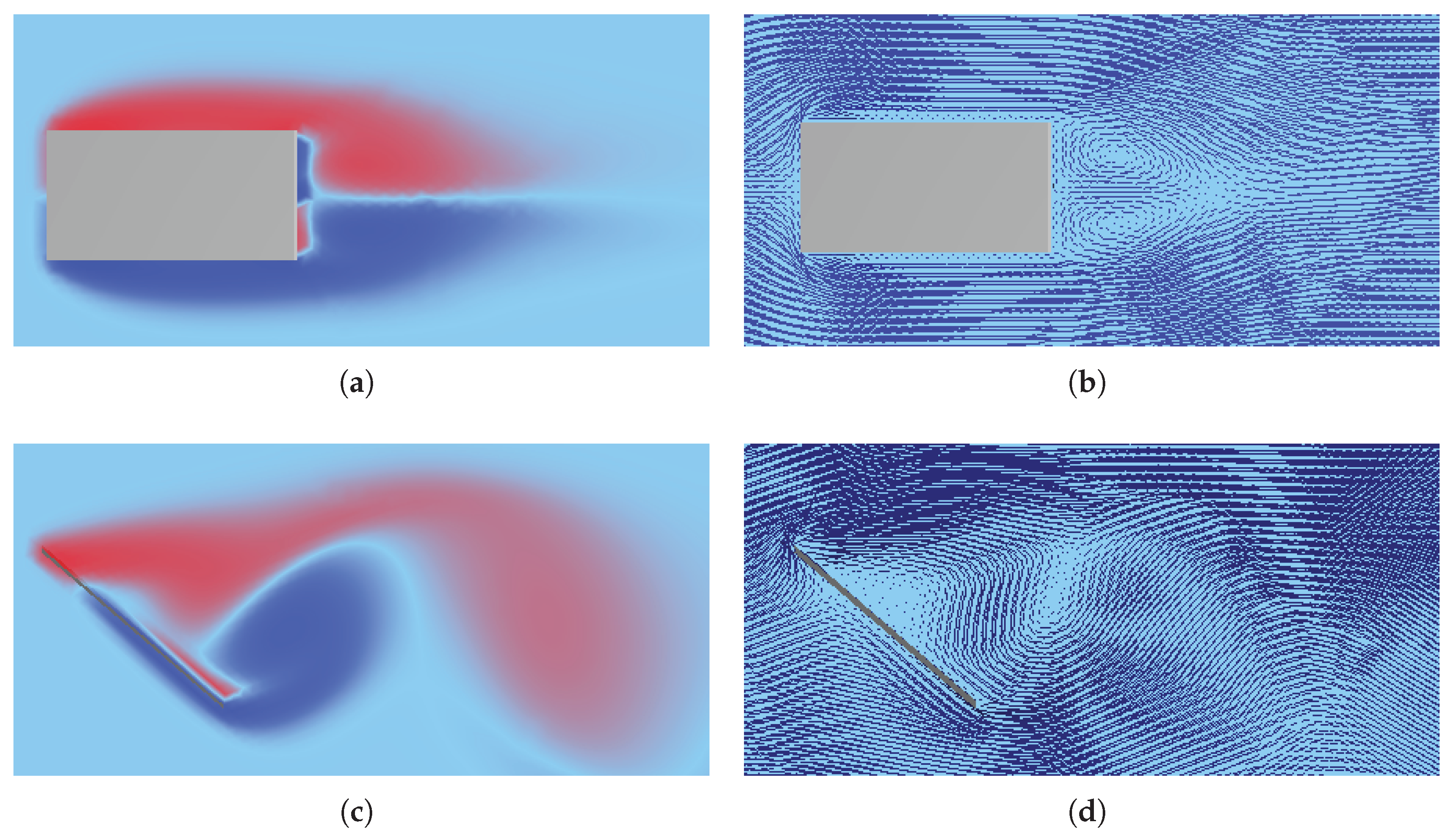
In numerical experiment Poisson equation was solved by FEM with continuous piecewise linear basis functions on triangles in a triangulated plane region with about 3600 nodes. Data for vorticity function w in right-hand side of (27) which satisfies integral restrictions (24) with $\rho \equiv 0$ was generated in AGVortex program from vorticity flow with no-slip condition. In Figure 1 there are presented vorticity and velocity of flows around rectangle and a line segment.

6. Discussion

Regarding the geometry of the exterior domain $\Omega$ in the current research its boundary consists of two connected components (including point at infinity). But presented approach can be extended to the case of more than two connected components, when the fluid flows through several solids. The relation on moments (24) will include superposition of several Riemann mappings which are taken by the number of solids. If these solids are far apart from each other, then (24) becomes an approximation of the no-slip condition for each object.

In exterior of the line segment the statement of the div-curl problem requires some explanation. In that case the line segment has "two sides" in some sense and no-slip condition must be imposed on both sides of it. It can be considered as a limiting case of ellipses which are divided into two parts and when its thickness goes to zero. The definition of the solution can be obtained via Riemann mapping of the div-curl problem into exterior of the disk, where we can correctly define the solution of the equation. Vorticity flow in In Figure 1 (c) breaks down into two parts with clock-wise rotation (red color) and counter clock-wise (blue color). These regions are separated by zero-vorticity line ($w=0$) which crosses through a line segment for reasons of symmetry.

Orthogonality relations can be extended to 3D domains. For example in case of the spherical solid they can be written using vector spherical harmonics. No-slip condition implies zero value of the curl’s normal component $(w,\mathbf{n})=0$ on the boundary when the rest tangent components of w must satisfy integral relations over exterior of the sphere.

7. Conclusions

Integral constraints (24) imposed on vorticity function w and divergence $\rho$ give unique solvability of the exterior div-curl problem with no-slip boundary condition around solid. It can be solved numerically by reducing to Poisson problem. This approach can be extended to flows around several streamlined solids.

For solenoidal flows no-slip condition generates a series of integral constraints on vorticity (orthogonality relations). Under these restrictions the div-curl problem can be solved in correct formulation with more typical boundary conditions - slip condition combined with zero circulation. The source of vorticity data, which satisfies such integral constraints can be derived by solving any equations of motion written in vorticity form which describe fluid dynamics - Stokes, Navier-Stokes, Boussinesq equations. And the div-curl problem becomes one of the steps of the numerical procedure in the planar computational fluid dynamics.

References

- L. Quartapelle and F. Valz-Gris, Projection conditions on the vorticity in viscous incompressible flows. Internat. J. Numer. Methods Fluids, 1(2), 129–144, (1981).
- G. Auchmuty and J. C. Alexander, L2 well-posedness of planar div-curl systems. Arch. Ration. Mech. Anal., 160, 91–134, (2001).
- M. Neudert and W. von Wahl, Asymptotic behaviour of the div-curl problem in exterior domains. Adv. Differ. Equ., 6(11), 1347–1376, (2001).
- B. B. Delgado and J. E. Macías-Díaz, An exterior Neumann boundary-value problem for the div-curl system and applications. Mathematics, 9, (2023).
- A. V. Gorshkov, On the unique solvability of the div-curl problem in unbounded domains and energy estimates of solutions. Theor. Math. Phys., 221, 1799–1812, (2024).
- A. V. Gorshkov, Associated Weber-Orr transform, Biot-Savart law and explicit form of the solution of 2D Stokes system in exterior of the disc. J. Math. Fluid Mech., 21(41), (2019).
- A. P. Calderón and A. Zygmund, On singular integrals. Amer. J. Math., 78(2), 289–309, (1956).
Figure 1.
Numerical results of flows around solid calculated in program AGVortex. (a) Vortex flow around rectangle. (b) Velocity field around rectangle. (c) Vortex flow around line segment. Zero-vorticity line () crosses through a line segment. (d) Velocity field around line segment.
Disclaimer/Publisher’s Note: The statements, opinions and data contained in all publications are solely those of the individual author(s) and contributor(s) and not of MDPI and/or the editor(s). MDPI and/or the editor(s) disclaim responsibility for any injury to people or property resulting from any ideas, methods, instructions or products referred to in the content. |
© 2025 by the authors. Licensee MDPI, Basel, Switzerland. This article is an open access article distributed under the terms and conditions of the Creative Commons Attribution (CC BY) license (http://creativecommons.org/licenses/by/4.0/).
Copyright: This open access article is published under a Creative Commons CC BY 4.0 license, which permit the free download, distribution, and reuse, provided that the author and preprint are cited in any reuse.