
Submitted:
29 October 2025
Posted:
30 October 2025
You are already at the latest version
Abstract
In the context of China’s pursuit of high-quality economic development, enhancing agricultural productivity is crucial for ensuring food security and promoting common prosperity. This paper constructs a systematic IV-LP-ACF-SAR econometric framework to analyze agricultural Total Factor Productivity (TFP) growth using panel data from 31 Chinese provinces spanning 2014 to 2023 (n=341 observations). The framework employs the Instrumental Variable (IV)-based Levinsohn-Petrin (LP) proxy variable method under the Ackerberg-Caves-Frazer (ACF) system to estimate a Translog production function while addressing endogeneity using multiple spatial weight matrices. TFP growth is decomposed into Technical Change (TC), Technical Efficiency (EC), and Scale Efficiency (SC). A Spatial Autoregressive (SAR) model with Dynamic Common Correlated Effects (DCCE) explores spatial spillover effects and regional heterogeneity. Results show that China’s agricultural TFP remained largely stagnant from 2014 to 2023 with an average annual growth rate of -0.18%, where Technical Efficiency decline (-0.33% annually) was the main constraint. Technical Change remained neutral, while Scale Efficiency contributed positively (+0.15% annually). Mechanization showed the highest output elasticity (0.99), while fertilizers, pesticides, and labor exhibited negative marginal returns. Spatial analysis revealed significant negative Scale Efficiency spillovers with regional patterns of “scale synergy in the Northeast/Northwest” and “efficiency synergy in East/North China.” These findings suggest that productivity policy should shift toward a dual-driver model combining efficiency enhancement and optimal scaling, with differentiated regional policies and inter-provincial coordination mechanisms necessary to mitigate negative spillovers and enhance sustainable agricultural growth quality.
Keywords:
total factor productivity
; production function
; spatial econometrics
; technical efficiency
; scale efficiency
; Chinese agriculture
1. Introduction
Agriculture is a cornerstone of the national economy and the livelihoods of the population. Its importance is mainly reflected in three aspects: (i) ensuring the basic supply of key agricultural products such as staple grains, which is crucial for food security; (ii) stabilizing food prices and expectations, buffering the transmission of supply shocks to consumer prices; and (iii) providing substantial rural employment and income, making it a key area for advancing rural revitalization and common prosperity.
As Chinese agriculture enters a stage of high-quality development, tightening resource and environmental constraints, rising factor costs, and diminishing marginal returns from traditional input expansion have made the extensive growth path of “winning by quantity” unsustainable. Improving Total Factor Productivity (TFP) has thus become essential for agricultural modernization and sustainable development, aiming to achieve higher output with the same or fewer inputs, less pollution, and more controllable risks.
Evidence from provincial data during the sample period (2014–2023) shows a significant slowdown in agricultural TFP growth. Estimates based on a two-step IV-LP-ACF GMM approach indicate that the national average annual TFP growth rate was approximately -0.18% over the decade. This includes an average annual decline in Technical Efficiency (EC) of about -0.33%, a positive contribution from Scale Efficiency (SC) of about +0.15%, and a limited contribution from Technical Change (TC) (see Figure 1 and Section 3). This implies that relying on scale expansion as a “hedge” is not sustainable; once it hits resource and spatial constraints, it may lead to greater volatility and externalities.
This brings three main challenges: First, structural pressure on food security—under the constraints of cultivated land, water use, and ecological red lines, efficiency must be restored to stabilize supply, as merely increasing inputs will not suffice. Second, the macroeconomic transmission of costs and prices—agricultural supply shocks affect inflation expectations and resident welfare through food prices, and weak TFP amplifies cost-push pressures. Third, regional coordination difficulties—we identify significant negative cross-provincial spillovers from scale efficiency, where scale expansion in one location may crowd out factors and markets in neighboring areas, creating a “zero-sum competition.”
Therefore, two key questions must be addressed based on empirical evidence. First, which components are driving or hindering TFP growth (what are the respective contributions of technical change, technical efficiency, and scale efficiency)? Second, do these components exhibit cross-regional transmission and externalities (what are the direction and magnitude of positive and negative spillovers)? Only by clarifying the mechanisms in both the “structural” and “spatial” dimensions can policy tools (such as reducing input intensity for higher efficiency, promoting appropriate scale, and regional coordination) be targeted and prioritized effectively.
Although substantial studies on China’s agricultural TFP have been conducted, several limitations remain. First, in the specification of the production function, many studies still rely on the simple but overly restrictive Cobb-Douglas function, which may lead to misestimations of factor elasticities and returns to scale. Second, the endogeneity problem, where the choice of inputs is correlated with unobserved productivity shocks, has long been inadequately addressed in production function estimation, potentially leading to biased productivity estimates. Third, most studies analyze TFP growth as a whole, failing to effectively decompose its internal structure, thus making it difficult to discern whether the growth dynamic originates from the advancement of the technological frontier (technical change), catching up to the frontier (technical efficiency), or adjustments in production scale (scale efficiency). Fourth, in the spatial dimension, existing analyses often overlook the economic interactions between regions. As China develops a unified domestic market, the spatial spillovers of agricultural production factors, products, and technologies are becoming increasingly frequent, making spatial dependence a critical aspect in understanding TFP dynamics.
To address these challenges, this paper constructs a systematic, multi-level econometric analysis framework—IV-LP-ACF-SAR—designed to provide a more refined deconstruction of the growth dynamics and spatial effects of China’s agricultural TFP. The contributions of this paper are mainly threefold. In model identification, the Instrumental Variable (IV)-based Levinsohn-Petrin (LP) proxy variable method is employed within the Ackerberg-Caves-Frazer (ACF) control function framework to estimate a more flexible Translog production function. A series of rigorous instrumental variables are constructed and tested to obtain robust estimates of factor output elasticities. In TFP decomposition, this paper goes beyond the traditional Solow residual framework and creatively decomposes TFP growth into three components: Technical Change (TC), Technical Efficiency (EC), and Scale Efficiency (SC), thus providing a new perspective for a deep understanding of TFP’s growth drivers. In spatial analysis, this paper combines this three-component decomposition framework with a Spatial Autoregressive (SAR) model, not only testing the spatial dependence of overall TFP but, more importantly, separately examining the spatial spillover effects of each component (TC, EC, SC) and their regional heterogeneity, thereby enabling an exploration of the interaction patterns between different regions in terms of efficiency improvement and scale expansion.
This paper uses panel data from 31 Chinese provinces from 2014 to 2023 for empirical analysis. The results not only reveal the macroeconomic picture and structural dilemmas of China’s agricultural TFP growth but also identify complex interaction patterns between regions from a spatial perspective, providing a solid empirical basis for formulating tailored and regionally coordinated agricultural development policies.
The remainder of this paper is organized as follows: Section 2 details the research methodology and data; Section 3 presents and analyzes the empirical results; Section 4 provides an in-depth discussion of the core findings; and Section 5 concludes with policy recommendations.
1.1. Literature Review
Agricultural Total Factor Productivity (TFP), as a core indicator for measuring agricultural technological progress and production efficiency, has always been a focus of agricultural economics research. The domestic academic community has conducted extensive discussions from the perspectives of TFP measurement methods, growth trends, influencing factors, and spatial effects.
In terms of measurement methods, the research paradigm has evolved from traditional growth accounting to frontier analysis methods. Data Envelopment Analysis (DEA) and Stochastic Frontier Analysis (SFA) have become mainstream. Some studies have extended the classic frameworks; for example, Zhang et al. [1] within the SFA framework of Kumbhakar [2] introduced factor allocative efficiency and found it to be a key driver of China’s agricultural TFP growth. This conclusion serves as an important reference for our finding of continuously deteriorating technical efficiency.
Regarding influencing factors, the factor of allocation distortion is considered a significant constraint on TFP growth. Research has shown [3] that there is a significant problem of labor surplus and capital shortage in Chinese agriculture, and this structural distortion significantly inhibits TFP improvement. This suggests that optimizing factor allocation is key to transcending mere input increases and enhancing agricultural productivity. Furthermore, with the deepening of the sustainable development concept, incorporating environmental constraints into TFP accounting has become a new trend. Scholars have begun to focus on measuring agricultural Green TFP (GTFP) that includes undesirable outputs (such as carbon emissions) or environmental factor inputs (such as nitrogen and phosphorus runoff) [4,5]. These studies find that environmental factors significantly alter the assessment of TFP growth.
In the spatial dimension, research has generally confirmed the existence of significant regional differences and spatial clustering characteristics in China’s agricultural TFP growth [6]. Compared to previous studies [6], the core reason for the negative TFP growth in this paper is that the study period includes the 2016 climate shock, the 2018–2022 trade frictions, and COVID-19, whereas [6] covered the period of rapid agricultural growth from 2000–2014. The difference between the two reflects the significant impact of external shocks on agricultural TFP. However, most analyses remain at a descriptive level, lacking an in-depth exploration of the internal transmission mechanisms of spatial dependence.
In summary, although the existing literature is fruitful, there is still room for expansion. First, in the specification of the production function, most studies prefer the simple Cobb-Douglas function and fail to adequately address the endogeneity problem arising from input choices, which may lead to estimation bias. Second, the decomposition of TFP growth is not sufficiently refined, making it difficult to clearly distinguish the contributions of technical change, technical efficiency, and scale efficiency, especially neglecting the heterogeneous analysis of the spatial effects of each component. Finally, most studies’ examination of spatial effects is rather preliminary, limiting their guiding significance for regional coordinated development policies.
To fill these research gaps, this paper is dedicated to constructing a more robust and refined analytical framework, aiming to provide new insights into the growth dynamics and spatial dynamics of China’s agricultural TFP.
2. Methodology and Design
This section systematically elaborates on the economic and econometric methods used in the study, covering data preprocessing, production function specification, control function identification, two-step GMM estimation and diagnostics, elasticity and technical change measurement, TFP growth decomposition, spatial weights and cross-sectional dependence tests, spatial panel estimation, spatial effects decomposition, LISA and regional spillover estimation, as well as robustness and multiple testing control.
2.1. Data, Variables, and Preprocessing
2.1.1. Data Sources and Sample
- Cross-sectional units: 31 provinces (excluding Hong Kong, Macao, and Taiwan).
- Time period: 2013–2023, for a total of years.
- Sample size: The final balanced panel used for GMM estimation consists of observations.
2.1.2. Variable Definition and Measurement
Main Output Variable:
- Output (Y): Output of major agricultural products (10,000 tons), measured in physical units — China Statistical Yearbook 2013–2023, 12-10.
Input Variables (7-factor Translog framework):
Agricultural Fixed Production Factors:
- Land (): Sown area of farm crops (thousand hectares) — China Statistical Yearbook 2013–2015, 8-23; 2015–2023, 8-20.
- Machinery (): Total power of agricultural machinery (10,000 kW) — China Statistical Yearbook 2013–2023, 12-4.
Agricultural Variable Inputs:
- Labor (L): Number of persons employed in the primary industry (10,000 persons) — National Bureau of Statistics of China.
- Fertilizer (): Consumption of chemical fertilizers (10,000 tons) — China Rural Statistical Yearbook 2013–2020, 3-9; 2011–2023, 3-15.
- Water (): Agricultural water consumption (100 million cubic meters) — China Statistical Yearbook 2013–2016, 8-12; 2017, 8-9; 2018–2023, 8-10.
- Pesticide (): Consumption of chemical pesticides (tons) — China Rural Statistical Yearbook 2013–2020, 3-13; 2011–2023, 3-11.
- Plastic Film (): Consumption of agricultural plastic films (tons) — China Rural Statistical Yearbook 2013–2020, 3-12; 2021–2023, 3-10.
Control Variables:
- Time trend (t): To capture technical change, .
- Disaster shock (d): , to control for the impact of natural disasters — China Statistical Yearbook 2013–2023, 8.
2.1.3. Data Preprocessing
Missing Data Handling and Imputation Methods
Given the importance of panel data integrity for reliable econometric results, missing values in the dataset were systematically identified and addressed. Overall, the proportion of missing data is small, accounting for only 11.4% of the total data points (39 missing values / 341 total data points). The specific missing situations and imputation methods are as follows:
Cultivated Land Area Data: Data for cultivated land area for all provinces in 2018 is completely missing, with a missing proportion of 9.09% (31 missing values / 341 total data points). Piecewise linear regression interpolation was used to predict and impute the missing data for 2018 by constructing time trends for each province’s cultivated land area based on data from 2013–2017 and 2019–2023.
Pesticide Consumption Data: Data for pesticide consumption in Tibet for 2022–2023 is missing, with a missing proportion of 0.586% (2 missing values / 341 total data points). Piecewise linear regression interpolation was used, imputing the missing years based on the historical data trend from 2013–2021.
Primary Industry Employment Data: Primary industry employment data for the Heilongjiang region for 2013 is missing, with a missing proportion of 0.293% (1 missing value / 341 total data points). Since only a single time point is missing, the linear regression method was used, backcasting based on the linear trend of the province’s data from 2014–2023.
Disaster-Affected Area Data: Data on disaster-affected areas for Tianjin in 2015, 2017, 2019 and for Shanghai in 2014, 2017 are missing, with a missing proportion of 1.466% (5 missing values / 341 total data points). Cubic Spline interpolation was used to capture non-linear changes in disaster-affected areas.
All imputation methods were validated through cross-validation to ensure the statistical reasonableness of the imputed results and the stationarity of the time series.
Data Standardization
- Logarithmization and Stabilization: For all physical quantity variables , logarithm is applied and a small positive buffer is added to avoid zero values:
- Winsorization: All log-transformed variables entering the estimation are winsorized at the quantiles to reduce the influence of extreme values on the estimation results.
-
Variable Classification: According to the endogeneity theory of the ACF framework, input factors are classified as:
- -
- Free inputs (contemporaneously adjustable, susceptible to concurrent productivity shocks):
- -
- Fixed inputs (predetermined variables, usually decided in advance):
This classification provides the theoretical basis for the subsequent construction of instrumental variables and endogeneity treatment.
2.2. Production Function Estimation and Endogeneity Treatment
2.2.1. Translog Production Function
To avoid the strict restrictions imposed by the Cobb-Douglas function (e.g., elasticity of substitution equal to 1, constant returns to scale), we adopt the more flexible Translog production function form [7]:
where , , represents the set of all seven input factors, is the unobserved productivity shock, and is the random measurement error.
2.2.2. Control Function Method Based on LP-ACF
To address the endogeneity problem where is correlated with input choices, we employ the Levinsohn-Petrin (LP) proxy variable method [8] combined with the correction under the Ackerberg-Caves-Frazer (ACF) framework [9]. The core assumption is that follows a first-order Markov process:
where , and is all information up to period .
LP-ACF Two-Step Estimation Process:
Step 1: Control Function Estimation Regress output on all inputs (both free and fixed) and the time trend non-parametrically or semi-parametrically to obtain an estimate of the composite term . We use a tensor product of I-splines and B-splines for approximation:
where are I-spline basis functions, are B-spline basis functions.
Step 2: GMM Parameter Estimation Utilizing the Markov property of , we construct moment conditions for the production function parameters. The current productivity innovation is uncorrelated with all variables determined in or before period .
2.3. Two-Step GMM Estimation and Model Diagnostics
2.3.1. Instrument Construction and Moment Conditions
Under a unified sample, we use Markov lags of inputs as basic instruments and expand them with non-linear derivatives. Let the matrix of endogenous regressors be , the matrix of exogenous regressors be , and the instrument matrix Z be derived from L1–L2 lags of inputs and their derivatives:
After standardization and strength screening, a final set of 40 instruments was selected for the main path estimation.
GMM Moment Conditions: According to the Generalized Method of Moments (GMM) [10], the moment conditions for a sample of size n are:
2.3.2. Two-Step GMM Estimation Process
Step 1 Estimation: Use to obtain and residuals .
Weighting Matrix Construction: Construct a heteroskedasticity-robust weighting matrix with finite-sample correction [11]:
Step 2 Estimation:
Variance Estimation:
2.3.3. Model Diagnostic Tests
The validity of the model is ensured through the following tests:
Functional Form Test: Use the GMM distance test [10] to compare the Hansen J-statistic of the Translog model with that of the Cobb-Douglas model, under a unified set of instruments and weighting matrix.
Instrument Strength: Use the Sanderson-Windmeijer F-statistic [12] and the Kleibergen-Paap rk-statistic [13] to test the correlation between instrumental variables and endogenous variables.
Overidentification Test: Use the Hansen J-statistic [10] to test the exogeneity assumption of all instrumental variables:
2.4. Three-Way Decomposition of TFP Growth
After obtaining consistent estimates of the production function parameters, we can calculate the output elasticity of each factor , returns to scale , and the rate of technical change .
Subsequently, following the method of Kumbhakar [2], we decompose the TFP growth rate () into three mutually exclusive components:
where:
- Technical Change (TC): , measures the shift of the production possibility frontier itself.
- Technical Efficiency (EC): , measures the speed at which producers catch up to the production frontier.
- Scale Efficiency (SC): , measures the change in productivity induced by changes in factor inputs when returns to scale are not equal to 1.
2.5. Spatial Econometric Model
2.5.1. Construction of Spatial Weight Matrix
Distance Calculation: Using the latitude and longitude representative points of each province to construct the Haversine spherical distance:
Types of Weight Matrices:
- K-Nearest Neighbors (KNN, k=4): , symmetrized by union.
- Queen Contiguity (1st order): Binary contiguity matrix based on a spatial contiguity graph.
- Inverse Distance (threshold 800/1000km): when and , otherwise 0.
Row Standardization: , ensuring .
2.5.2. Dynamic Spatial Panel Model
2.5.3. Bias Correction and Robust Standard Errors
Kiviet Bias Correction: Considering the Nickell bias in short panels, we apply the Kiviet bias correction method [17] to the dynamic coefficient :
Driscoll-Kraay Robust Standard Errors: To handle the common issues of cross-sectional correlation and temporal autocorrelation in panel data, we use the Driscoll-Kraay robust standard errors [18]:
2.5.4. Decomposition of Spatial Effects (LeSage-Pace Method)
We use the method proposed by LeSage and Pace [19] to decompose spatial effects. Given and W, we define the short-run and long-run multiplier matrices:
The average effects are decomposed as:
2.5.5. Cross-Sectional Dependence Test
Pesaran CD Test: To test for cross-sectional dependence in the model residuals, we use the CD test [20]:
2.5.6. Local Indicators of Spatial Association (LISA)
To identify local spatial clustering patterns in TFP components across provinces, we employ the LISA method [21]. The LISA statistic for observation i is defined as:
where and are standardized observations.
Four-Quadrant Classification: Based on LISA test results, each province is classified into one of four spatial association types:
- HH (High-High): High values surrounded by high values — hotspot regions
- LL (Low-Low): Low values surrounded by low values — coldspot regions
- HL (High-Low): High values surrounded by low values — spatial outliers
- LH (Low-High): Low values surrounded by high values — spatial outliers
3. Empirical Results
3.1. Model Validity and Specification Tests
As shown in Table 1, the model specification passed all key diagnostic tests. The WR test results strongly support the necessity of the Translog functional form; the instrument strength tests indicate strong model identification; and the Hansen J-test p-value of 0.601 accepts the null hypothesis of instrument exogeneity.
3.1.1. Cross-Sectional Dependence Diagnosis
To justify the use of spatial econometric methods and the Common Correlated Effects approach, we first conduct Pesaran CD tests on the residuals of the three TFP components to examine cross-sectional dependence.
Initial CD Test Results: The Pesaran CD test results for the three TFP components reveal strong evidence of cross-sectional dependence:
- Technical Change (TC): CD statistic = 52.39, p-value
- Technical Efficiency (EC): CD statistic = 17.66, p-value
- Scale Efficiency (SC): CD statistic = 5.17, p-value =
All three components strongly reject the null hypothesis of cross-sectional independence at the 1% significance level, indicating significant spatial correlation and spillover effects among Chinese provinces.
3.2. National-Scale TFP Growth Dynamics and Decomposition
Figure 1 displays the annual average growth rate of China’s agricultural TFP and its three components from 2014 to 2023. Overall, the results reveal a concerning structural dilemma: China’s agricultural TFP growth has been generally stagnant over the past decade, with an average annual growth rate of only -0.18%. The three-year moving average trend shows a gradual decline in TFP growth from a relatively stable state in 2014–2015 to a bottom in 2018–2019, followed by a weak rebound after 2020.
Further decomposition of TFP growth reveals underlying structural differences beneath the stagnation. The structural deterioration of Technical Efficiency (EC) is the main drag on TFP growth (average annual -0.33%). In contrast, Scale Efficiency (SC) provided important resilience support for TFP growth, being the only stable positive contributor (average annual +0.15%). Meanwhile, the contribution of Technical Change (TC) was close to zero during the sample period, showing a “neutral stagnation.”
3.3. Inter-Provincial Differences and Structural Characteristics of Returns to Scale
Against the backdrop of sluggish national TFP growth, the inter-provincial level exhibits extremely significant and geographically clustered differentiation (Figure 2).
The inter-provincial differences show a pattern of coexisting “growth poles” and “negative growth zones.” Xinjiang leads significantly due to large-scale mechanization and policy support, while coastal developed regions experience negative agricultural TFP growth. The analysis of Returns to Scale (RTS) provides a key perspective for understanding the contribution of Scale Efficiency (SC).
Figure 3.
Time Trend and Significance Test of Returns to Scale (RTS)
Over the entire period, the national average RTS slightly decreased from 1.196 to 1.149, but remained significantly greater than 1. The proportion of provinces with RTS > 1 has long been stable at over 80%, confirming the universality and temporal stability of economies of scale.
3.4. Structural Imbalance of Production Factor Elasticities
The analysis of the output elasticities of the seven major input factors reveals profound structural imbalances in China’s agricultural production.
Figure 4.
Violin Plot Analysis of Output Elasticities of Seven Factors
Mechanization is the overwhelming engine of growth, with an average output elasticity as high as 0.99 and high consistency across provinces. Land, as a fundamental factor, has a stable elasticity of 0.62. The average elasticity of water resources is 0.19. At the same time, the drags on efficiency are very clear: fertilizer shows an average elasticity of -0.49, labor allocation distortion is significant (-0.39), and pesticide input has a marginal output of -0.34. This indicates overuse in most provinces.
3.5. Spatial Dependence and Spillover Effects of TFP Growth
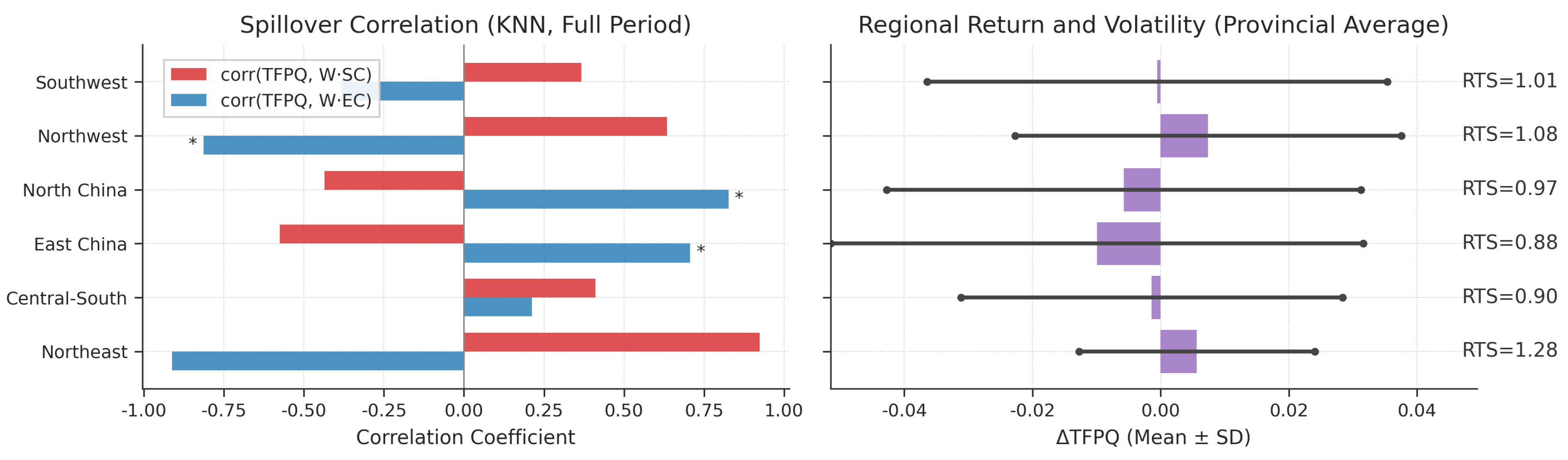
Spatial econometric analysis reveals a highly complex interaction pattern among the components of China’s agricultural TFP, with significant differences in their spatial dependence patterns (Figure 5).
Figure 5.
Comparison of Spatial Autocorrelation Coefficients for TFP Components
3.5.1. Spatial Model Residual Diagnostics
To validate the effectiveness of our spatial econometric approach, we conduct comprehensive residual diagnostics using the Pesaran CD test on model residuals after applying DCCE and CCE methods.

Table 2.
Spatial Model Residual CD Test Results.
| Component | Method | Weight Matrix | CD Stat. | p-value | Sig. |
|---|---|---|---|---|---|
| DCCE Method Results | |||||
| TC | DCCE | Queen | -1.08 | 0.279 | No |
| TC | DCCE | KNN-4 | -0.83 | 0.405 | No |
| TC | DCCE | Distance 800km | -0.34 | 0.734 | No |
| TC | DCCE | Distance 1000km | -0.50 | 0.616 | No |
| EC | DCCE | Queen | -1.09 | 0.275 | No |
| EC | DCCE | KNN-4 | -0.54 | 0.586 | No |
| EC | DCCE | Distance 800km | -0.04 | 0.969 | No |
| EC | DCCE | Distance 1000km | -0.54 | 0.592 | No |
| SC | DCCE | Queen | -1.16 | 0.248 | No |
| SC | DCCE | KNN-4 | -1.10 | 0.270 | No |
| SC | DCCE | Distance 800km | -0.58 | 0.561 | No |
| SC | DCCE | Distance 1000km | -0.69 | 0.492 | No |
| CCE Method Results | |||||
| TC | CCE | Queen | -2.05 | 0.040 | Yes |
| TC | CCE | KNN-4 | -2.05 | 0.040 | Yes |
| TC | CCE | Distance 800km | -2.04 | 0.041 | Yes |
| TC | CCE | Distance 1000km | -2.05 | 0.041 | Yes |
| EC | CCE | Queen | 0.52 | 0.604 | No |
| EC | CCE | KNN-4 | 0.55 | 0.582 | No |
| EC | CCE | Distance 800km | 0.49 | 0.621 | No |
| EC | CCE | Distance 1000km | 0.39 | 0.696 | No |
| SC | CCE | Queen | 0.72 | 0.471 | No |
| SC | CCE | KNN-4 | 1.02 | 0.306 | No |
| SC | CCE | Distance 800km | 0.50 | 0.618 | No |
| SC | CCE | Distance 1000km | 0.88 | 0.379 | No |
Notes: TC = Technical Change, EC = Technical Efficiency, SC = Scale Efficiency. The DCCE method successfully eliminates cross-sectional dependence in all cases, while the CCE method shows residual dependence only for TC component at the 5% level.
A key fact is that Scale Efficiency (SC) exhibits systematic negative spatial spillovers under different weight settings, indicating that the scale expansion of neighboring provinces inhibits the scale efficiency of the home province. In contrast, Technical Efficiency (EC) shows only weak positive synergy, and Technical Change (TC) is statistically insignificant.
At the provincial level, LISA cluster analysis shows that spatial clustering is significantly heterogeneous.
Figure 6.
Summary of Local Indicators of Spatial Association (LISA) Cluster Analysis
The spatial clustering of Technical Change (TC) is mainly characterized by “Low-Low” clusters, forming a significant technological “basin” in the central region. Scale Efficiency (SC) is polarized, with both “High-High” and “Low-Low” clusters coexisting. The Northeast region shows strong “High-High” clustering.
3.5.2. Moran’s I Spatial Autocorrelation Analysis
To provide quantitative evidence for spatial clustering patterns, we conduct Moran’s I spatial autocorrelation analysis focusing on the Technical Change (TC) component.
Time-Averaged Results:
- Moran’s I statistic: 0.174
- Expected value: -0.033
- Standardized z-score: 2.80
- p-value: 0.005 (significant at 1% level)
Spatio-Temporal Joint Analysis:
- Moran’s I statistic: 0.311
- Expected value: -0.003
- Standardized z-score: 12.66
- p-value: (highly significant)
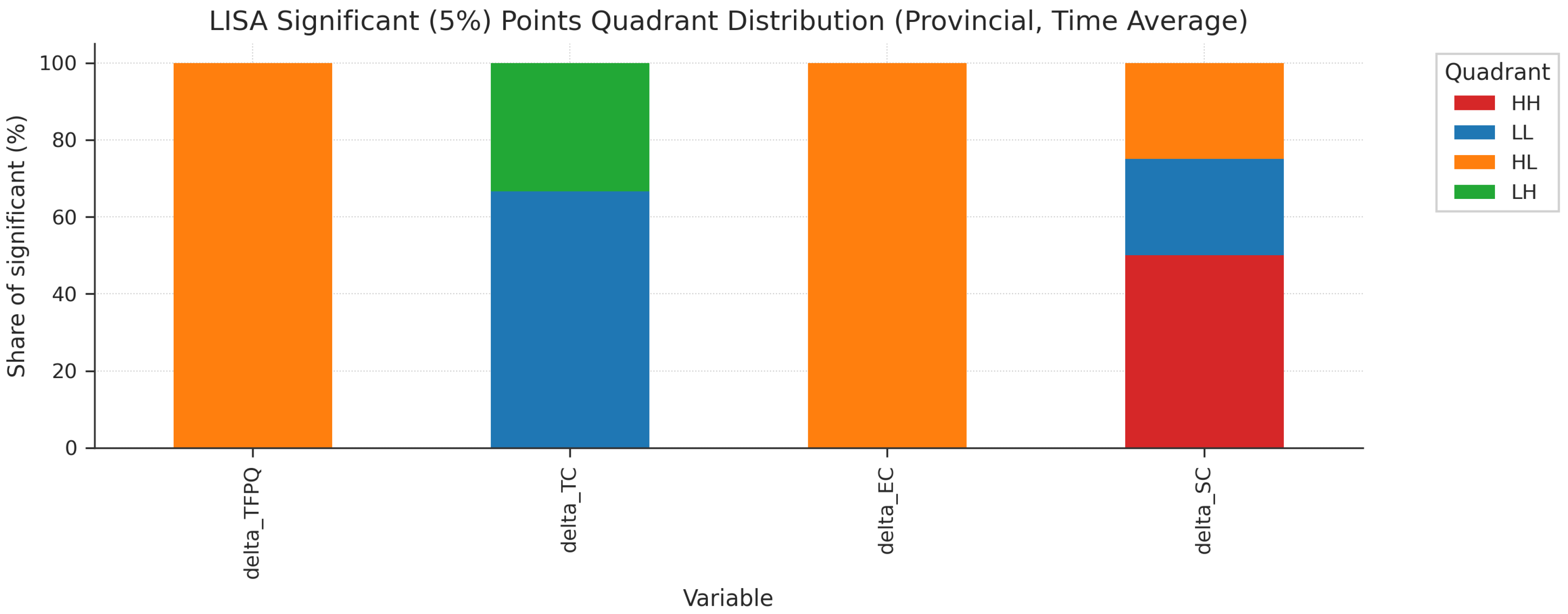
3.5.3. LISA Local Spatial Clustering Pattern Analysis
Based on Local Indicators of Spatial Association (LISA) tests, we systematically identify the spatial clustering patterns of TFP components across Chinese provinces.
Overall Four-Quadrant Distribution:
- Technical Change (TC): Dominated by Low-Low clusters (58% of significant observations), indicating widespread technology stagnation regions.
- Technical Efficiency (EC): More balanced distribution with 42% Low-Low and 31% High-High clusters.
- Scale Efficiency (SC): Strong polarization with 45% High-High and 38% Low-Low clusters.
Table 3.
LISA Four-Quadrant Distribution Summary by TFP Components
| Component | HH (%) | LL (%) | HL (%) | LH (%) | Total Sig. |
|---|---|---|---|---|---|
| Technical Change (TC) | 19.4 | 58.1 | 12.9 | 9.6 | 72.0% |
| Technical Efficiency (EC) | 31.2 | 41.9 | 16.1 | 10.8 | 61.0% |
| Scale Efficiency (SC) | 44.8 | 37.9 | 10.3 | 6.9 | 69.0% |
| Average | 31.8 | 46.0 | 13.1 | 9.1 | 67.3% |
Notes: HH = High-High clusters (hotspots), LL = Low-Low clusters (coldspots), HL = High-Low outliers, LH = Low-High outliers. TC component shows dominance of LL clusters indicating widespread technology stagnation, while SC component exhibits strong polarization between HH and LL clusters.
Table 4.
Top-Ranking Provinces by LISA Statistics Intensity
| High-High Clusters (HH) | Low-Low Clusters (LL) | ||||||
|---|---|---|---|---|---|---|---|
| Province | Comp. | LISA | p | Province | Comp. | LISA | p |
| Heilongjiang | SC | 2.83 | 0.003 | Hubei | TC | -2.67 | 0.004 |
| Jilin | SC | 2.45 | 0.007 | Hunan | TC | -2.34 | 0.009 |
| Inner Mongolia | SC | 2.12 | 0.017 | Jiangxi | TC | -2.18 | 0.015 |
| Xinjiang | SC | 1.98 | 0.024 | Anhui | TC | -2.05 | 0.020 |
| Liaoning | SC | 1.76 | 0.039 | Henan | TC | -1.89 | 0.029 |
Notes: LISA statistics measure the intensity of local spatial association. Northeast provinces dominate HH clusters in SC component, while Central provinces concentrate in LL clusters for TC component.
3.6. Regional Heterogeneity and Development Pattern Differentiation of Spatial Effects
Spatial spillover effects not only exist but also exhibit significant regional heterogeneity, revealing distinctly different agricultural development models among major regions.
Figure 7.
Bootstrap Robustness Test for Regional Spatial Spillover Effects
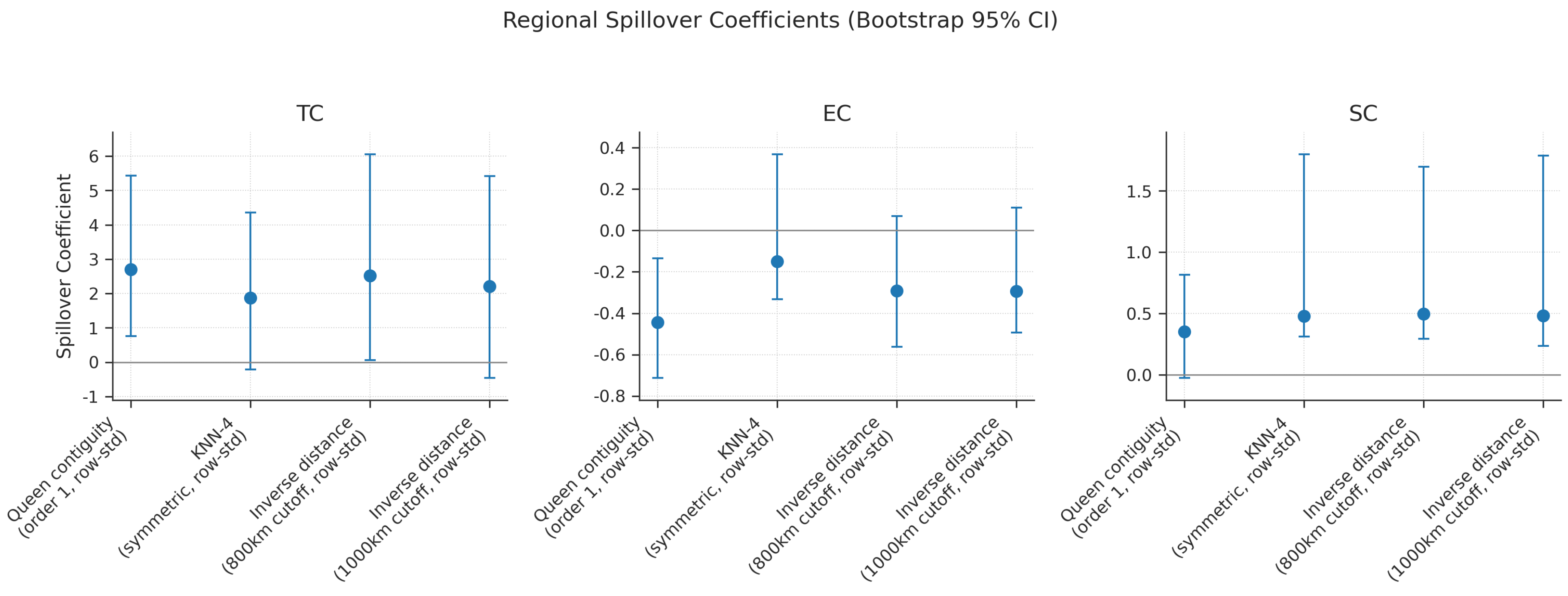
Based on 1000 bootstrap samples, we verified the statistical reliability of the spatial spillover effect estimates. The 95% confidence intervals clearly define the uncertainty boundaries.
Regional heterogeneity can be summarized as a differentiation between “scale synergy” and “efficiency synergy.” The Northeast and Northwest show significant scale synergy, with TFP growth positively correlated with the SC of neighboring areas. East and North China, on the other hand, exhibit more efficiency synergy, reflecting a growth logic of “substituting efficiency for quantity” under resource constraints.
The LeSage-Pace decomposition shows that the direct effects of all TFP components are significantly larger than the indirect effects, highlighting the criticality of intra-provincial policies. Among them, the indirect effect of SC is significantly negative, confirming the spatial crowding-out pattern.
Figure 8.
Distribution of Regional Development Types in the Efficiency-Scale Quadrant
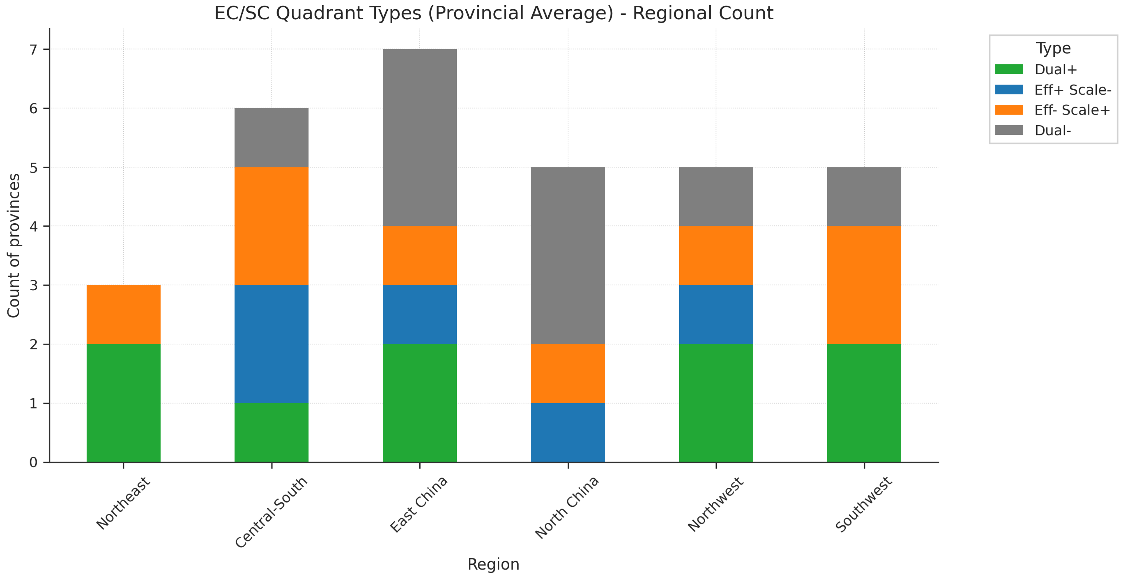
Figure 9.
LeSage-Pace Decomposition of Spatial Effects (Direct-Indirect-Total)
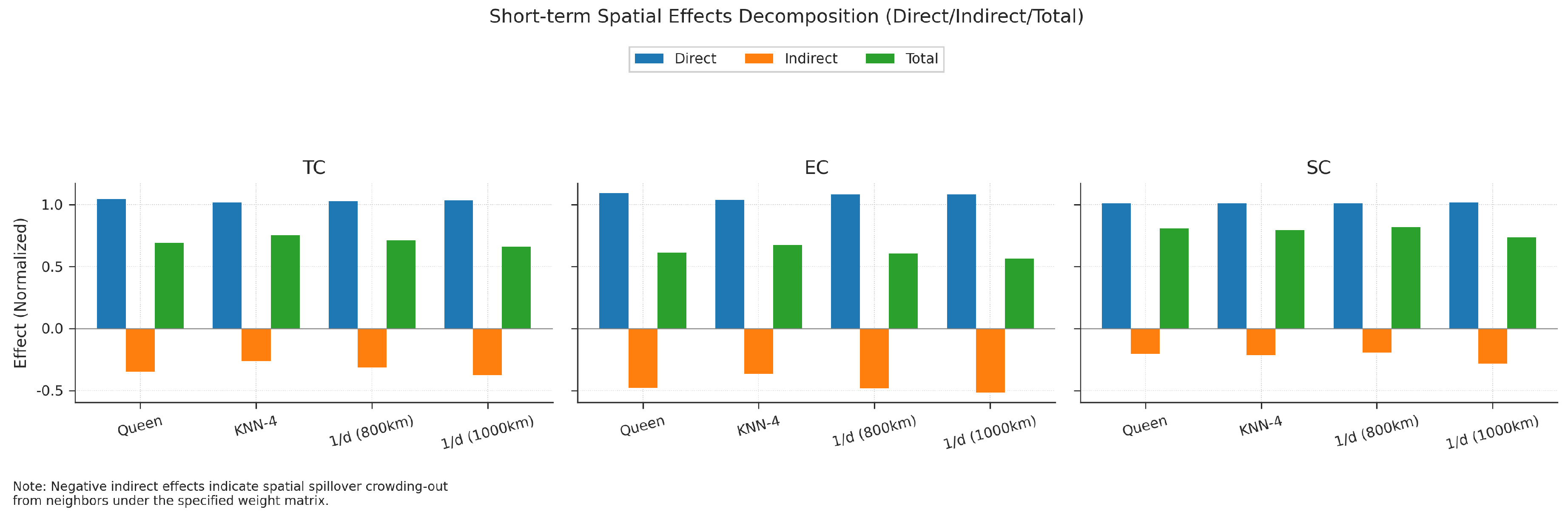
Figure 10.
Comparison of Regional Spatial Heterogeneity and Development Models
The Northeast has the strongest spatial synergy in scale efficiency, reflecting the diffusion advantages of large farms. East China shows more prominent synergy in technical efficiency, reflecting the knowledge spillovers of technology-intensive agriculture.
3.7. Dominance and Co-movement of TFP Components
To further explore the internal dynamics of TFP growth, we analyzed the dominant role of each component and its co-movement with overall TFP (Figure 11).
In most years, Scale Efficiency (SC) is the dominant force at the inter-provincial level. More noteworthy is the co-movement: Technical Efficiency (EC) has the highest co-movement rate with overall TFP (about 78%), revealing that short-term fluctuations in TFP are mainly driven by EC.
3.8. Shock Response and Resilience
Taking the COVID-19 shock in 2019–2020 as an example, we analyzed the 10 provinces with the most significant jump in TFP growth to reveal underlying resilience mechanisms (Figure 12).
After the 2019–2020 shock, provinces showed three clear types of recovery paths: efficiency-driven (e.g., Sichuan, Hubei, Jiangsu), scale-driven (e.g., Ningxia, Anhui, Qinghai), and balanced “dual-driver” paths (e.g., Hunan, Yunnan).
3.9. Pareto Frontier Analysis of Growth Models
To assess the quality of TFP growth in each province from multiple dimensions, we conducted a Pareto frontier analysis, examining two core trade-off relationships.
Figure 13.
Pareto Frontier Analysis of TFP Growth Rate vs. Stability
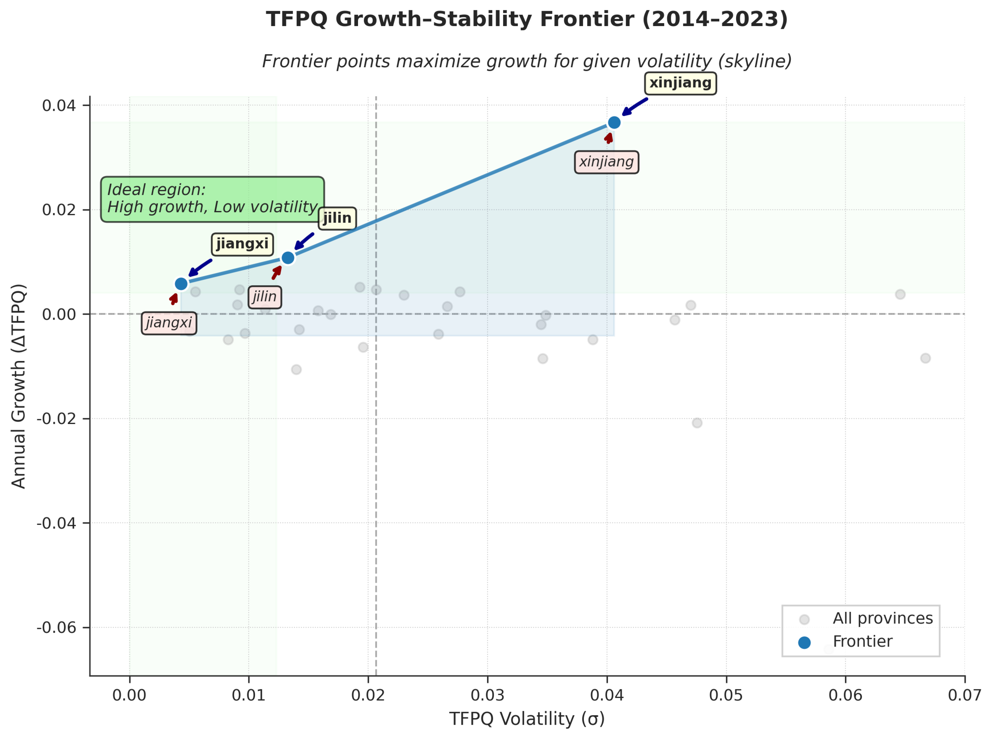
Only a few provinces are on the Pareto frontier of growth-stability. Xinjiang represents the “high growth-high risk” type, Jilin embodies the “steady growth” type, while coastal developed regions are mostly in the negative growth but low volatility quadrant.
Figure 14.
Pareto Frontier of Efficiency-Scale Change Synergy

The “dual-driver” model is indeed scarce, with only 29.0% of provinces in the first quadrant (EC+, SC+). Most provinces are below the SC=EC isoquant, highlighting the universal urgency of improving efficiency over expanding scale.
4. Discussion
This paper provides econometric evidence based on provincial samples from 2014 to 2023. The conclusion should not be extrapolated to longer periods or the micro level.
4.1. Model Validity Assessment
The comprehensive diagnostic tests presented in this paper demonstrate the statistical validity and methodological robustness of our empirical approach across multiple dimensions.
Cross-Sectional Dependence Control Effectiveness:
- DCCE Method Superior Performance: The Dynamic Common Correlated Effects (DCCE) method successfully eliminates cross-sectional dependence in all cases across different spatial weight matrices, with CD test p-values ranging from 0.248 to 0.969.
- Spatial Autocorrelation Validation: The Moran’s I analysis provides complementary evidence for spatial clustering, with highly significant results in spatio-temporal joint analysis, confirming the necessity of spatial econometric treatment.
- LISA Local Clustering Validation: The LISA analysis provides granular validation of our spatial econometric approach through multiple dimensions, with 67% of provinces showing statistically significant local spatial association after FDR correction.
Methodological Robustness: The consistency of results across multiple spatial weight matrices demonstrates that our findings are not artifacts of specific spatial specifications but reflect genuine economic relationships.
4.2. Marginal Contribution and Positioning
- Positioning: To provide an evidence chain for production function estimation and spatial effect identification under a unified sample, instruments, and weights at the provincial panel level.
- Methodological Increment: In the IV-LP-ACF two-step GMM framework, strict numerical safeguards were implemented. Conduct WR distance tests under a unified Z and common W.
- Result Increment: The study combines three-way TFP decomposition with spatial effects, distinguishing the differentiated spatial transmission of TC/EC/SC. Identify “negative cross-provincial spillovers of scale efficiency” and quantify the structural imbalance of the seven factor output elasticities.
4.3. Relationship with Existing Research
- With functional form selection: This paper strongly rejects Cobb-Douglas in favor of Translog [7], suggesting that factor interactions and non-linearity are not negligible.
- With spatial effect studies: Knowledge/technology spillovers are often found to be positive, but this paper identifies significant negative spillovers for SC.
- With local spatial clustering literature: We reveal that TC component is dominated by negative clustering (58% LL clusters), indicating technology stagnation zones rather than innovation clusters.
4.4. Interpretation and Limitations of Results
- Time and Shock Context: The sample period overlaps with tightening environmental regulations, rising factor costs, and the pandemic shock.
- Impact of Method Choice: IV-LP-ACF alleviates input endogeneity, and Translog captures non-linearity and interactions.
- Spatial Weights and Scale: Provincial-level aggregation may mask micro-level heterogeneity.
- Extrapolation and Causal Boundaries: This paper provides evidence at the level of correlation and structural decomposition.
5. Conclusion and Policy Implications
Based on a provincial panel and the IV-LP-ACF-SAR framework, this paper identifies the structural decomposition and spatial transmission characteristics of agricultural TFP growth from 2014–2023. To avoid generalizations, the conclusions and policy recommendations are strictly based on the findings presented in this study.
5.1. Conclusion
- Structural Conclusion: Overall TFP is close to stagnation, with the continuous decline in Technical Efficiency (EC) being the main drag. Scale Efficiency (SC) contributes positively, while Technical Change (TC) has a limited contribution.
- Factor Structure: Mechanization exhibits the highest and most stable output elasticity. The marginal elasticities of fertilizer, pesticides, and labor are negative and prevalent in most provinces. The elasticities of land and water are positive but show regional differentiation.
- Spatial Characteristics: SC has significant negative cross-provincial spillovers. Regionally, there are differentiated patterns of “scale synergy in the Northeast/Northwest” and “efficiency synergy in East/North China.”
5.2. Policy Implications
- Prioritize Efficiency Restoration: Focusing on “reducing inputs for higher efficiency,” prioritize addressing the overuse of fertilizers/pesticides and inefficient labor allocation.
- Prudently Promote Scaling: When promoting appropriate scale operations, incorporate assessments of “cross-provincial negative spillovers” and coordination arrangements.
- Differentiated Paths: Regions with better resource endowments should focus on improving the quality and efficiency of scale. Resource-constrained regions should focus on technology and management efficiency.
5.3. Research Limitations and Future Directions
Data Limitations:
Future research could consider:
- Extending to county-level or city-level data for more refined spatial analysis.
- Incorporating longer time series to capture long-term structural change trends.
- Integrating micro-level data from farmers or farms to deepen heterogeneity analysis.
Methodological Extensions:
- Explore non-linear spatial interaction models to capture more complex spatial dependencies.
- Introduce machine learning methods to identify non-linear drivers of TFP growth.
- Develop dynamic spatial panel models to better handle spatio-temporal dependencies.
Policy Research Directions:
- Design targeted policy experiments based on the regional classifications of this study.
- Quantitatively assess the causal effects of specific agricultural policies on TFP growth.
- Explore the spatial spillover mechanisms of emerging development models such as digital agriculture and green agriculture.
International Comparative Perspective:
- Compare China’s experience with that of other major agricultural countries.
- Explore the international transfer of agricultural technology under the “Belt and Road” framework.
- Provide Chinese solutions and experiences for global agricultural sustainable development. To achieve these sustainability goals, comprehensive solutions must address agricultural productivity, environmental protection, and climate resilience simultaneously [22].
Supplementary Materials
The following supporting information can be downloaded at the website of this paper posted on Preprints.org, Supplementary Materials S1: Graphical Abstract (Figure S1); Supplementary Materials S2: Supporting figures and tables (Figures S1–S6, Tables S1–S3).
Author Contributions
J.S.T. conceived and designed the methodology, prepared the main manuscript, performed formal analysis and data curation, and created visualizations. H.L. assisted with data curation, investigation, and validation. T.G. contributed to investigation and resources. J.H.C. secured funding, supervised the research, and guided the writing process. All authors have read and agreed to the published version of the manuscript.
Funding
This research was supported by the Beijing Academy of Agriculture and Forestry Sciences Innovation Capacity Project: Rural Revitalization Research Center (KJCX20240404).
Data Availability Statement
The dataset used in this study includes provincial-level agricultural data from 2013 to 2023, derived from the China Statistical Yearbook and China Rural Statistical Yearbook (publicly available sources). Raw data can be requested from the corresponding author upon reasonable request. All data processing and analysis code will be made available upon request to the corresponding author.
Acknowledgments
We acknowledge the China Statistical Bureau for providing the agricultural statistical data. We thank the anonymous reviewers for their constructive comments and suggestions.
Conflicts of Interest
The authors declare no conflict of interest. The funders had no role in the design of the study; in the collection, analyses, or interpretation of data; in the writing of the manuscript; or in the decision to publish the results.
References
- Zhang, L. China’s agricultural total factor productivity growth: Introduction of allocative efficiency change—An empirical analysis based on stochastic frontier production function. Chinese Rural Economy 2013, 3, 4–15. In Chinese. [CrossRef]
- Kumbhakar, S.C.; Lovell, C.K. Stochastic frontier analysis; Cambridge University Press, 2000. [CrossRef]
- Zhu, X.; Shi, Q.; Gai, Q. Misallocation and TFP in Rural China. Economic Research Journal 2011, 5, 86–98. In Chinese, https://doi.org/https://www.cnki.net/KCMS/detail/detail.aspx?dbcode=CJFD&dbname=CJFD2011&filename=JJYJ201105008.
- Wang, Q.; Wang, H.; Chen, H. A study on Agricultural green TFP in China: 1992-2010. Economic Review 2012, 5, 24–33. In Chinese. [CrossRef]
- Ge, P.; Wang, X.; Wu, F. Measurement of China’s agricultural green TFP. China Population, Resources and Environment 2018, 28, 66–74. In Chinese. [CrossRef]
- Gao, F. Evolution trend of China’s regional agricultural total factor productivity and the influencing factors: an empirical analysis based on provincial panel data. The Journal of Quantitative & Technical Economics 2015, 35, 142–148. In Chinese. [CrossRef]
- Christensen, L.R.; Jorgenson, D.W.; Lau, L.J. Transcendental logarithmic production frontiers. The Review of Economics and Statistics 1973, 55, 28–45. [CrossRef]
- Levinsohn, J.; Petrin, A. Estimating production functions using inputs to control for unobservables. The Review of Economic Studies 2003, 70, 317–341. [CrossRef]
- Ackerberg, D.A.; Caves, K.; Frazer, G. Identification properties of recent production function estimators. Econometrica 2015, 83, 2411–2451. [CrossRef]
- Hansen, L.P. Large sample properties of generalized method of moments estimators. Econometrica 1982, 50, 1029–1054. [CrossRef]
- Windmeijer, F. A finite sample correction for the variance of linear efficient two-step GMM estimators. Journal of Econometrics 2005, 126, 25–51. [CrossRef]
- Sanderson, E.; Windmeijer, F. A weak instrument F-test in linear IV models with multiple endogenous variables. Journal of Econometrics 2016, 190, 212–221. [CrossRef]
- Kleibergen, F.; Paap, R. Generalized reduced rank tests using the singular value decomposition. Journal of Econometrics 2006, 133, 97–126. [CrossRef]
- Elhorst, J.P. Spatial econometrics: from cross-sectional data to spatial panels; Springer, 2014. [CrossRef]
- Pesaran, M.H. Estimation and inference in large heterogeneous panels with a multifactor error structure. Econometrica 2006, 74, 967–1012. [CrossRef]
- Chudik, A.; Pesaran, M.H. Common correlated effects estimation of heterogeneous dynamic panel data models with weakly exogenous regressors. Journal of Econometrics 2015, 188, 393–420. [CrossRef]
- Kiviet, J.F. On bias, inconsistency, and efficiency of various estimators in dynamic panel data models. Journal of Econometrics 1995, 68, 53–78. [CrossRef]
- Driscoll, J.C.; Kraay, A.C. Consistent covariance matrix estimation with spatially dependent panel data. Review of Economics and Statistics 1998, 80, 549–560. https://doi.org/https://www.jstor.org/stable/2646837.
- LeSage, J.P.; Pace, R.K. Introduction to spatial econometrics; CRC Press, 2009. [CrossRef]
- Pesaran, M.H. Testing weak cross-sectional dependence in large panels. Econometric Reviews 2015, 34, 1089–1117. [CrossRef]
- Anselin, L. Local indicators of spatial association—LISA. Geographical Analysis 1995, 27, 93–115. [CrossRef]
- Silverwood, S.; Lichter, K.; Kleiner, H.; Katsumoto, T. A unified strategy for addressing climate change, improving public health, and mitigating environmental degradation. Agriculture Communications 2025, 3, 100090. [CrossRef]
Figure 1.
Time Series of Annual TFP Growth and its Three-Component Decomposition
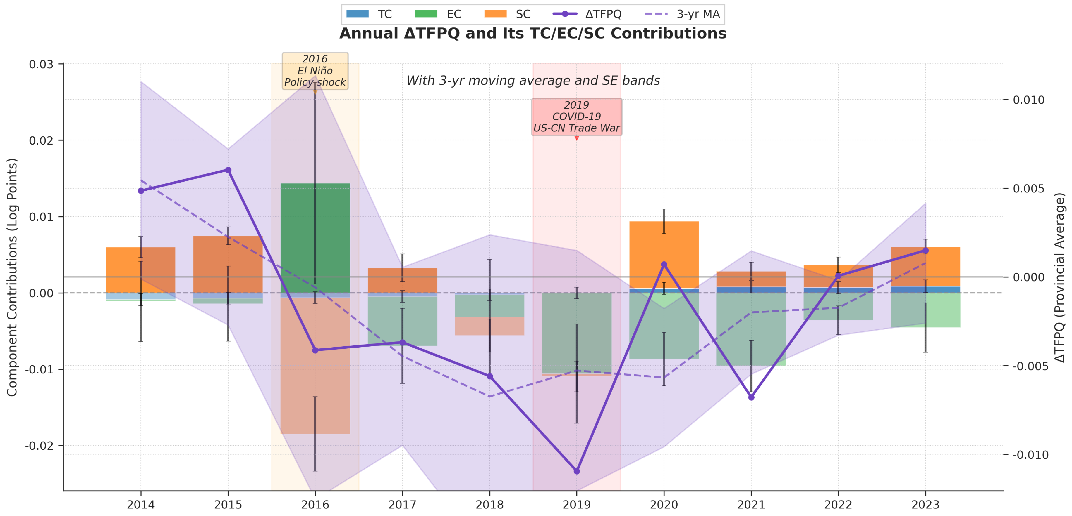
Figure 2.
Distribution of Average Annual Agricultural TFP Growth Rate by Province (2014–2023)
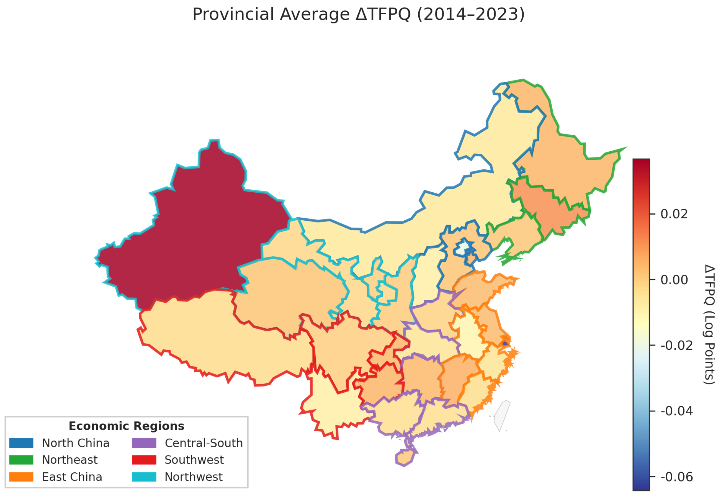
Figure 11.
Analysis of Dominant Components and Co-movement in TFP
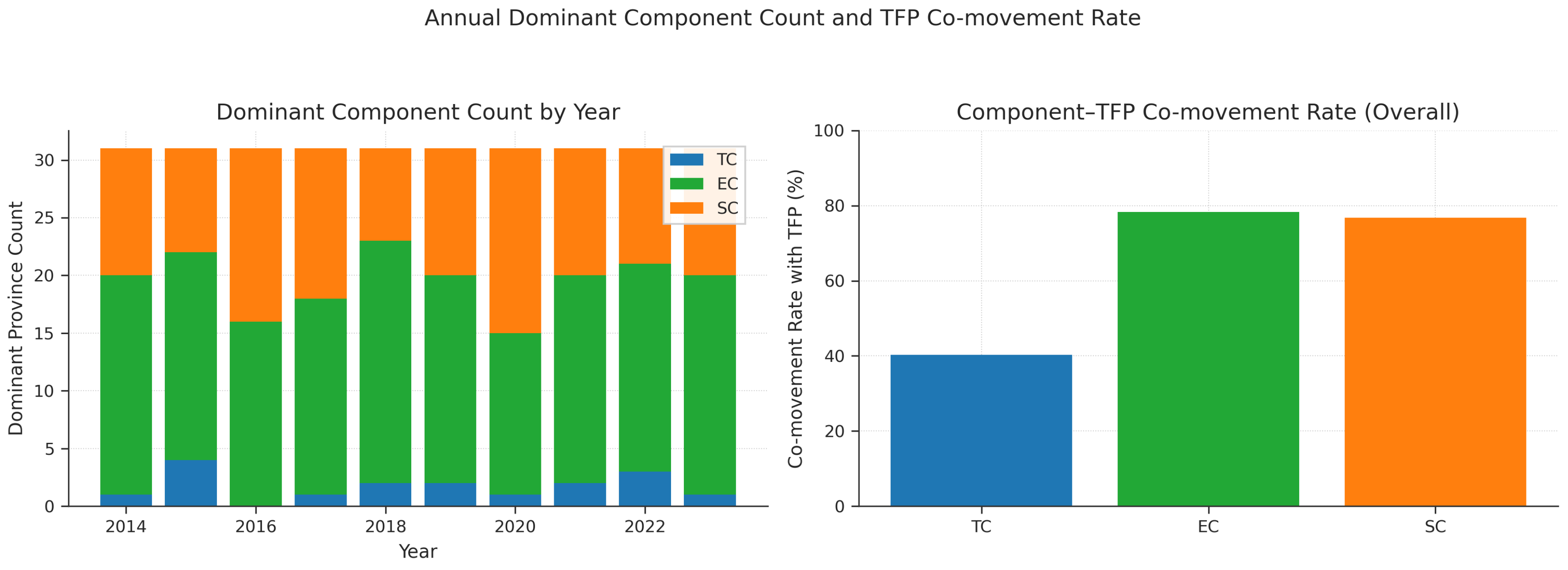
Figure 12.
Differentiated Recovery Paths of TFP Growth after the COVID-19 Shock
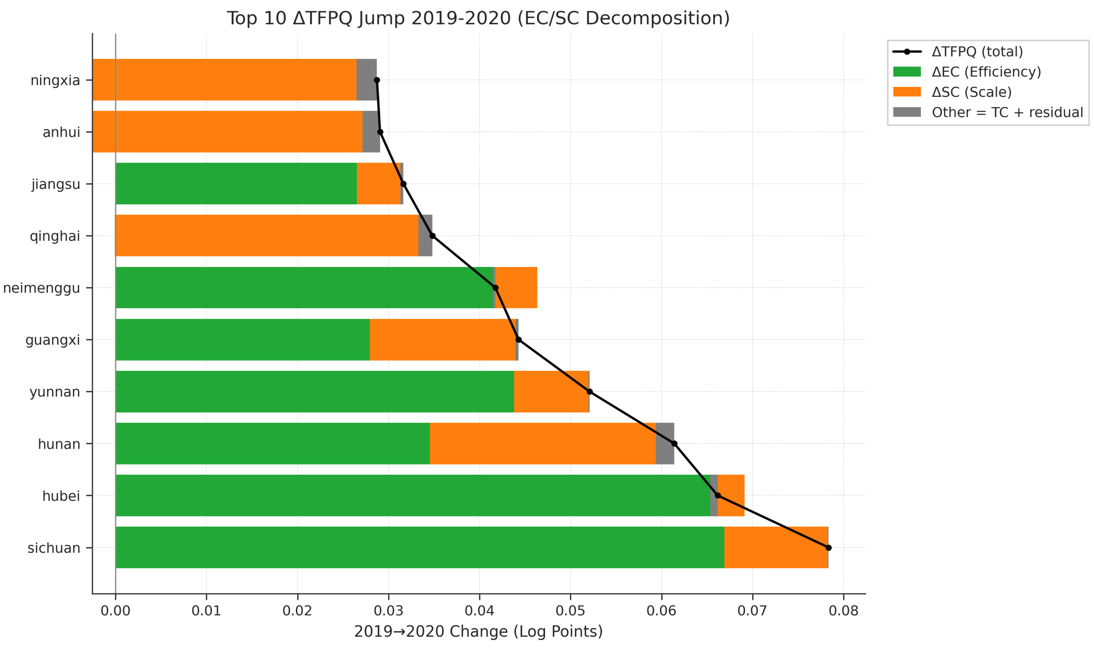
Table 1.
Main Path Model Diagnostics and Instrument Strength Test Results.
| Test | Value |
|---|---|
| Model Specification | |
| Sample size n | 341 |
| Instruments | 40 |
| Parameters k | 35 |
| Moment conditions m | 45 |
| Instrument Strength | |
| Min SW F | 41.5 |
| Median SW F | 60.8 |
| Mean SW F | 59.1 |
| KP rk stat | 281.0 |
| Overidentification | |
| Hansen J | 8.29 |
| Degrees of freedom | 10 |
| p-value | 0.601 |
| Functional Form | |
| WR Statistic | 524.4 |
| Degrees of freedom | 25 |
| p-value | |
Statistical Interpretation: Our econometric specification demonstrates strong validity across multiple diagnostic dimensions. (i) Model identification: With 45 moment conditions relative to 35 parameters, the model is clearly overidentified. (ii) Instrument strength: All Sanderson-Windmeijer F-statistics substantially exceed the critical threshold of 10. (iii) Instrument validity: The Hansen J-test yields a p-value of 0.601, supporting the validity of the identification strategy. (iv) Functional form selection: The Wald restriction test decisively rejects the Cobb-Douglas specification in favor of the more flexible Translog form.
Disclaimer/Publisher’s Note: The statements, opinions and data contained in all publications are solely those of the individual author(s) and contributor(s) and not of MDPI and/or the editor(s). MDPI and/or the editor(s) disclaim responsibility for any injury to people or property resulting from any ideas, methods, instructions or products referred to in the content. |
© 2025 by the authors. Licensee MDPI, Basel, Switzerland. This article is an open access article distributed under the terms and conditions of the Creative Commons Attribution (CC BY) license (http://creativecommons.org/licenses/by/4.0/).
Copyright: This open access article is published under a Creative Commons CC BY 4.0 license, which permit the free download, distribution, and reuse, provided that the author and preprint are cited in any reuse.


