Submitted:
28 October 2025
Posted:
29 October 2025
You are already at the latest version
Abstract
With the upgrading of geostationary meteorological satellites, their capabilities in Convective Initiation (CI) identification have been enhanced. To improve the applicability of the ARGI-based CI algorithm in central and eastern China, this study uses Fengyun-4A data, integrates radar and precipitation data to construct a True_CI dataset, and defines False_CI events (satellite-identified events without radar or precipitation signals) for comparative analysis. The results show that True_CI events tend to have longer durations, larger cloud cluster areas, and lower central cloud-top brightness temperature (BT) during development. It exhibits distinct features such as reduced differences between water vapor and infrared channels, increased cloud optical thickness, and ice-phase transformation 30 minutes before CI occurrence—features absent in False_CI events. Based on these comparisons, a new CI definition on satellite cloud imagery is proposed, and a set of reference thresholds is formulated, targeting cloud-top cooling, increased optical thickness, and ice-phase transitions. The evaluation of the Defined_CI events (defined using the CI definition) via True_CI events indicates that the CI definition on satellite cloud imagery proposed in this study is reliable, and suggests that further research on the pre-CI environmental conditions of weak convection is needed. Supported by hyperspectral data or numerical model products, such research will help clarify which cloud clusters are prone to developing into convective weather.
Keywords:
Fengyun-4A satellite
; convective initiation definition
; brightness temperature
; central and eastern China
1. Introduction
Severe convective weather is the primary manifestation of sudden and disastrous weather events, encompassing hail, thunderstorm winds, tornadoes, and short-duration heavy precipitation [1,2,3,4,5,6]. Its occurrence often results in significant loss of life and property, and even has tremendous social impacts. In the process of severe convective weather warning and prediction, the identification and forecasting of convective initiation (CI) play a crucial role [7,8].
CI refers to a specific state in the early stages of severe convective weather, marking the onset of convective activity [9]. The traditional definition of CI is the moment when a Doppler weather radar first detects pixels with reflectivity factors ≥35 dBZ generated by convective clouds [10,11,12,13]. However, weather radar measures precipitation by detecting the scattering effect of precipitation particles on electromagnetic waves. This means that when radar detects echoes above 35 dBZ, precipitation may have already started on the ground. In contrast, the core technique for CI identification using satellites lies in leveraging the high temporal frequency observational advantage of geostationary meteorological satellites to monitor rapidly growing convection [14]. Theoretically, this enables satellites to monitor the onset of convection earlier than radars, thereby truly identifying the convective initiation phase. With the gradual improvement of satellite observation resolution, many studies focus on using satellite data to identify and forecast CI [10,15,16,17,18,19].
Maddox [20] first to propose using a threshold of brightness temperature (BT) to detect CI. Later, Setvák and Doswell [21] linked infrared channel temperature difference thresholds to cloud-top phase states and physical characteristics, while Strabala et al. [22] further explored this area. The principle of the infrared BT threshold method is clear and easy to operate, but it has the problem of low recognition accuracy. Usually, setting the threshold too low or too high can cause missed judgments or false alarms. To improve the effectiveness of the threshold method, more thresholds have been introduced for convective cloud monitoring. Mecikalski and Bedka [15] proposed the cloud object-based Satellite Convection Analysis and Tracking (SATCAST) algorithm based on data from the Geostationary Operational Environmental Satellite (GOES), and further conducted extended research thereafter [16]. The SATCAST algorithm includes eight indicators such as infrared cloud-top BT, the temporal trend of infrared cloud-top BT, differences in infrared cloud-top brightness temperatures, and others. The SATCAST algorithm currently only utilizes the spectral channels of the current GOES series satellites. While it can detect 90% of CI, it also has a relatively high false alarm rate. A typical example is its frequent misclassification of pixels adjacent to mature convective systems as new CI clusters during actual forecasting operations. This limitation stems from its single-pixel-based object tracking and verification approach, where the continuous development or rapid movement of anvil regions in mature convective systems leads to erroneous identification of edge pixels.
Sieglaff et al. [18] developed the UWCI algorithm based on the concept of box-averaged. The algorithm utilizes the average brightness temperature difference between two consecutive time blocks to roughly identify convective cloud clusters. It then employs seven criteria to eliminate non-convective pixels and identifies pixels that meet the cloud-top cooling rate as CI. This algorithm is simple, rapid, and efficient. However, it is prone to misjudgment in cases with horizontal cloud movement and complex multi-layer clouds.
Zhuge and Zou [19] utilized five different channels and their combinations from the Himawari-8 satellite to form eight indicators for determining the occurrence of convection, which showed good early warning effects in the Fujian region of China. Many studies have shown that the threshold for satellite detection of CI is not fixed and can be influenced by factors such as the season and geographical characteristics of the region [23].
Notably, beyond the challenge of establishing a unified threshold standard, there remains no consensus on a CI definition specifically tailored to satellite data. This gap hinders the accuracy of satellite-based CI identification, especially when distinguishing events that will develop into impactful weather. Against this backdrop, the present study is grounded in the understanding that the core of CI identification resides in the physical signals of convective motion—specifically deepening cloud thickness, sharp declines in cloud-top temperature, and changes in cloud-top phase state—all of which can be captured through multi-spectral comprehensive analysis techniques [14].
This study differs from existing work by prioritizing the differentiation between “True CI” and “False CI”: True CI refers to events that will eventually develop into strong convective precipitation, while false CI denotes misidentified cases. To ensure the authenticity of our target CI, we integrate radar-identified CI events and precipitation data for cross-validation, a step that addresses the limitation of previous studies which relied solely on satellite data. Specifically, this study aims to analyze the characteristic differences between genuine convective initiation cloud clusters and commonly misidentified ones across various satellite channel parameters; it also seeks to evaluate how effectively satellite channels characterize the cloud-top properties of developing cumulus clouds, and ultimately to establish a new CI definition for identifying CI with a focus on genuine CI that progresses to strong convection.
This paper is organized as follows. Section 2 provides a brief description of the data and method employed in this paper. Section 3 presents the characteristics of CI events and the evolution of satellite channel parameters prior to CI onset. Definitive criteria for CI in satellite cloud imagery are presented in Section 4, the main conclusions are drawn in section 5.
2. Materials and Methods
2.1. Data Description
This study utilizes data from the Advanced Geosynchronous Radiation Imager (ARGI) aboard the Fengyun-4A satellite to identify and analyze CI features. Launched on December 11, 2016, Fengyun-4A is China’s geostationary meteorological satellite dedicated to comprehensive atmospheric observations. Since March 2018, these data have been available for download from the Fengyun Satellite Remote Sensing Data Service Network (https://satellite.nsmc.org.cn/DataPortal/cn/home/index.html). Fengyun satellite datasets have been widely employed in meteorological research, with their quality gaining universal recognition [23,24].
Specifically, this study uses infrared BT data from Fengyun-4A, which were acquired by ARGI, the primary optical payload onboard the satellite. ARGI is equipped with 3 visible channels and 11 infrared channels, among which the infrared absorption and window channels were utilized in this research (Table 1). The data have a spatial resolution of 4 km at the satellite’s nadir point, with temporal resolutions of 15 minutes for full-disk observations and 5 minutes for the China region.
Additionally, this study incorporates radar reflectivity measurements from China’s S-band New Generation Doppler Weather Radars (INRAD). These radars are deployed over land areas in central and eastern China, with observational records covering April to September 2018. As shown in Figure 1, the study region spans latitudes 20.5° N to 40° N and longitudes 105° E to 124° E. Notably, composite reflectivity in this context refers to the maximum reflectivity value across all elevation angles.
2.2. Algorithm Description for Identifying CI
Building on the traditional satellite-based CI identification method, this study developed a single-channel algorithm for the rapid identification and tracking of CI by referring to Li Shanshan’s approach [24]. Additionally, we obtained satellite-derived CI labeled data from Fengyun-4A satellite data. The method consists of three parts: First, BT threshold below 273 K at the 10.7-μm band is used to identify convective cloud clusters from satellite data. Then, a dynamic threshold-based area overlap method is employed, where the variable threshold rate of overlapping is determined based on statistical rate of overlapping values for each cloud cluster group to assess whether cloud clusters between consecutive time intervals are matched. Finally, CI is determined based on the 15-minute cooling rates over a continuous 30-minute period.
Although this method has made efforts to minimize the false alarm rate and improve the CI detection rate using satellite data, it still cannot guarantee that all satellite-identified CI labels correspond to genuine CI events. We cross-referenced the satellite-identified CI label data with radar observations and ground-based precipitation measurements to differentiate genuine CI events from satellite misidentifications (false positives). The steps are described below.
Firstly, the satellite-derived CI events are matched with radar-identified CI events within a spatio-temporal window of 30 minutes before and after the satellite-triggered CI event time and a spatial radius of 20 km, in order to eliminate false alarms and generate satellite-radar matched CI events. The radar-identified CI events were tracked and identified using the area overlap method and the sliding cross-validation method based on the criteria of eight grid points with echo intensities greater than or equal to 35 dBZ.
Secondly within a spatial-temporal window of 60 minutes after the satellite CI trigger and extending 2km outside the CI cloud clusters movement zone, the satellite-derived CI events are also matched with precipitation data to generate satellite-precipitation matched CI events.
Lastly, the two matching results are combined to form a comprehensive identification of CI events. Furthermore, using a calibration system and a back-to-back verification method by forecasters, the CI annotation results are revised, resulting in a high-resolution and reliable CI annotation dataset. In total, 5,888 CI events were identified using the above-described CI identification method over the central and eastern regions of China from April to September of 2018. We hereby define these as True Convective Initiation (True_CI) events. Concurrently, we have defined 3,585 events that were identified as CI by satellite but were neither radar-identified CI nor matched with ground precipitation as False Convective Initiation (False_CI) events.
3. Statistical Characteristics of CI
3.1. Lifetime, Areas, BT
Through tracking all samples, it was found that the duration of True_CI events, from identification to dissipation or merger, primarily ranged from 1 to 2 hours for 33% of the samples. The second most common duration was less than 1 hour, while a significant portion (approximately 38%) lasted between 2 and 6 hours. This indicates that True_CI events can sustain development and last for hours. In comparison, False_CI events had a shorter lifespan, with most lasting no more than 1 hour, representing convective cloud clusters that failed to develop.
The ratio of initial area to maximum area also corroborated this observation. We calculated the ratio of the initial area of convective cloud clusters for CI events to their maximum area during development, multiplied it by 10, and examined the distribution of this “10×Ratio” for True_CI events and False_CI events (Figure 2). In Figure 2a, the histogram reveals that most samples cluster in the “10×Ratio” range of 0–2, with a sharp decline thereafter, and the kernel density curve peaks sharply in this interval, signifying a strong concentration. This means the initial area of convective cloud clusters for True_CI events is consistently far smaller than their maximum area. In contrast, for False_CI events, the histogram of the initial-to-maximum area ratio shows a wider distribution of “10×Ratio”, with samples spread from 0 to around 10, and the kernel density curve has a lower, smoother peak, reflecting greater data dispersion. This suggests that convective cloud clusters associated with True_CI events tend to undergo more substantial development and expansion compared to those linked to False_CI events.
This study used BT≤273K at the 10.7-μm band as the thresholds to identify a convective object. Therefore, initial minimum BT for both types of events clustered around 260-270K (Figure 3). However, during their development, only those convective cloud clusters associated with True_CI events will continue to cool, often reaching a point where the minimum BT drops below 221 K, a threshold used to identify severe convective objects [20,21]. This pronounced cooling indicates that True_CI-related convective systems possess stronger development potential and can evolve into more intense convective forms. In contrast, the minimum BT of False_CI events is typically around 260K and rarely drops below 241K, a threshold used by several authors to identify and extract convective objects [20]. Such a characteristic suggests that False_CI events tend to be less vigorous in their development, with convective activity that is relatively weak and short-lived compared to True_CI events.
There are also some individual cases where they exhibit similar duration, maximum areas, and minimum BT throughout the tracking process, but are identified as entirely opposite types (True_CI or False_CI) due to their different performance on radar or precipitation.
Figure 4 present two tracked convective cloud clusters with similar characteristics: one observed in Hubei, China, on June 10, 2018, and the other in Shanxi on August 18, 2018. To help understand, the convective cloud cluster tracked on June 10 is labeled as CI event “A”, while that on August 18th is “B”. Event A developed from a 2-pixel cloud cluster, reached a maximum area of 41 pixels before merging with other clouds, and lasted for 60 minutes. The minimum BT at its core decreased from 270 K initially to 248 K, meeting our satellite-based CI identification criteria. However, only some scattered radar composite reflectivity echoes of less than 20 dBZ were detected, and no surface precipitation occurred within an hour. By contrast, Event B exhibited a similar development pattern. Its cloud cluster expanded from 2 pixels to 39 pixels, with the core minimum BT decreasing from 272 K to a minimum of 261 K, and the convective cloud cluster persisted for 83 minutes. But its radar and precipitation observations were markedly different. Although there were visual inconsistencies between radar and satellite observations, distinct echoes exceeding 35 dBZ were still detected at the location of Event B via radar composite reflectivity. During the subsequent 1-hour cloud tracking period, 2.4 mm of precipitation was recorded at the surface.
Such a contrast reveals the essential difference in observational perspectives between radar and satellite—a difference that thus further highlights the limitations of the single-channel threshold method. Radar uses a bottom-up penetrative detection mode, focusing on the “essential attributes” of cloud interiors: e.g., the concentration and size of precipitation particles in the middle and lower layers. Satellites, by contrast, primarily capture macro-scale cloud-top features (e.g., BT, cloud cluster area, duration) from a top-down perspective. This top-down view prevents observation of key internal cloud factors, e.g., whether sustained updrafts exist in the middle and lower layers to support particle growth, or if there is sufficient water vapor to form large-sized precipitation particles.
We therefore need to conduct further analysis to identify other distinguishing satellite-based characteristics that support cloud cluster continuous development and trigger convective weather events.
3.2. Channel Characteristics of CI
To address the above-mentioned analysis need, and specifically to help understand the evolution of CI events prior to their occurrence, This study conducted an analysis of channels 9-14 and their dual- or triple-channel combinations. Although theoretically, a large number of interest fields can be constructed through dual- or triple-channel combinations, numerous studies [13,25,26] have shown that many of these fields possess overlapping physical attributes. Through an analysis of channels 9-14 and their various combinations, we have discovered that, apart from the BT at 10.7-μm (which we utilize for extracting CI events), there are precisely three additional interest fields that demonstrate distinctive characteristics preceding the occurrence of CI. In this paper, we delve into these four infrared interest fields (listed in Table 2) to gain a comprehensive understanding of the development characteristics of convective cloud clusters prior to the occurrence of CI from a satellite perspective. To avoid the blurring of the spectral signals, the magnitudes of the 4 interest fields are estimated using an average of the 25% of pixels with the coldest values of Tb, 10.7 within the convective cloud clusters associated with CI events. The variations in these fields provide us with a clearer understanding of cloud-top height, phase changes within clouds, and other aspects [19], thereby providing a detailed description of atmospheric states and cloud-top properties.
The following (Figure 5) displays the distribution of the 4 interest fields at 15-minute intervals, ranging from 60 minutes prior to the event up until the moment of its occurrence. The decrease in BT at the 10.7-μm band for both True_CI events and False_CI events indicates that their cloud-top heights are both rising. BT variations in the 10.7-μm band (Figure 5a) are relatively consistent and exhibit no significant differences between True_CI events and False_CI events prior to CI onset, primarily because we rely on the cooling rate of this channel for satellite-based CI identification. However, in scenarios where a lower tropospheric inversion layer exists and cumulus clouds undergo rapid development to the point of breaking through this inversion layer, the cooling rate of cloud-top temperature detected by the 10.7-μm band tends to be abnormally elevated. Such an anomaly may lead to the misclassification of non-convective systems as CI events, which also explains why the utilization of single-channel satellite data results in a high false alarm rate in CI identification.
The BT difference between the 7.1-μm water vapor channel and the 10.7-μm infrared channel (i.e., Tb, 7.1-Tb, 10.7) are an indicator of cloud-top height relative to lower-troposphere. During convective weather events, higher cloud tops correspond to reduced water vapor content within the cloud. This reduction in water vapor leads to an increase in the BT recorded by the water vapor channel, causing it to approach the BT observed in the infrared channel. When cloud tops are elevated to the upper troposphere, the Tb, 7.1-Tb, 10.7 difference transitions from negative values to near-zero values. As illustrated in Figure 5b, a distinct disparity in Tb, 7.1-Tb, 10.7 is evident between True_CI events and False_CI events. For True_CI events, the Tb, 7.1-Tb, 10.7 values begin to increase 45 minutes prior to the CI event, followed by a rapid ascent starting 30 minutes beforehand. In contrast, False_CI events exhibit an increase in Tb, 7.1-Tb, 10.7 only 15 minutes prior to the perceived CI event, with the magnitude of this increase being smaller than that observed in True_CI events. Consequently, the integration of 10.7-μm band data and the Tb, 7.1-Tb, 10.7 difference can effectively mitigate false CI identifications caused by the rapid growth of cumulus clouds.
The BT difference between the 12.0-μm and 10.7-μm channels (Tb, 12.0-Tb, 10.7), known as the split-window channel technique, is commonly employed to characterize cloud optical thickness. For thin clouds, Tb, 12.0-Tb, 10.7 values exhibit significantly negative magnitudes, with these values increasing as cloud thickness increases [22]. For the majority of True_CI events, Tb, 12.0-Tb, 10.7 values increased rapidly 30 minutes prior to CI and reached peak values at the moment of CI occurrence, indicating progressive cloud thickening (Figure 5c). In contrast, False_CI events showed no significant increases in Tb, 12.0-Tb, 10.7 values. This finding suggests that cumulus clouds with rapidly ascending cloud tops, such as the misidentified False_CI events, do not necessarily exhibit corresponding increases in optical thickness. Consequently, Tb, 12.0-Tb, 10.7 can serve as a reliable indicator for distinguishing between False_CI events and True_CI events.
The tri-channel BT difference involving the 8.5-μm, 12.0-μm, and 10.7-μm bands (i.e., Tb, 8.5 +Tb, 12.0-2Tb, 10.7) is utilized to infer the cloud-top phase [26,27]. Ice clouds typically exhibit larger magnitudes in the Tb, 8.5 -Tb, 10.7 difference compared to the Tb, 12.0-Tb, 10.7 difference, whereas water clouds generally display the opposite pattern, with smaller Tb, 8.5 -Tb, 10.7 differences relative to Tb, 12.0-Tb, 10.7 differences. Specifically, at the cloud top, the tri-channel difference yields positive values for ice-phase clouds and negative values for water-phase clouds.
The statistical results (Figure 5d) indicate that for True_CI events, the tri-channel difference (i.e., Tb, 8.5 +Tb, 12.0-2Tb, 10.7) begins to exhibit a significant increasing trend 30 minutes prior to CI occurrence. For some True_CI events, this difference has already become positive by the time CI occurs, indicating a gradual ice-phase transformation at the cloud top. In contrast, False_CI events only show an increase in this difference at the moment of their misclassification as CI events, with peak values lower than those observed for True_CI events. This suggests that no significant ice-phase transformation has occurred within these cumulus clouds. Therefore, incorporating the tri-channel difference into satellite-based CI identification algorithms will effectively improve the accuracy of such assessments.
4. Definitive Criteria for CI in Satellite Imagery
True_CI events not only exhibit pronounced cloud-top cooling rates but also demonstrate increased optical thickness relative to the lower troposphere and undergo ice-phase microphysical transitions, characteristics absent in False_CI events.
Operationally, this study defines Convective Initiation in satellite cloud imagery as the initial detection of well-developed moist convective pixels that exhibit significant feature differentiation from the surrounding cloud field. We integrate previously established satellite-based CI identification criteria with the 25th percentile thresholds (i.e., thresholds exceeded or met by 75% of samples). These thresholds are derived from data of True_CI events captured 15 minutes prior to CI initiation, as illustrated by the boxplot of Figure 5. Collectively, these integrated criteria constitute the reference thresholds for identifying True CI (hereafter referred to as the CI definition criteria):
Initial number of pixels ≥ 2, initial area cloud cluster ≥ 64 km2 (the area of 2 pixels at a 4 km spatial resolution of Fengyun-4A Satellite)
The text continues here.
Bulleted lists look like this:
- BT at the 10.7 µm band ≤ 273 K, initial with continuous cooling over 30 minutes at a rate of ≥ 4 K (15min)-1.;
- BT difference between the 7.1-μm band and 10.7-μm band (BTD7.1-10.7) > -28 K;
- BT difference between the 10.7-μm band and 12.0-μm band (BTD12.0-10.7) > -2 K;
- Tri-channel difference of 8.5-μm band, 12.0-μm band and 10.7-μm band (BTD8.5 + 12.0 - 2*10.7) > -3.5K.
Through the statistical analysis of the differences between the actual values of BTD7.1-10.7, BTD12.0-10.7, and BTD8.5 + 12.0 - 2*10.7 for True_CI events at 15 minutes prior to CI initiation and the corresponding thresholds specified in the CI definition criteria, it is observed that most True_CI events satisfy the threshold requirements. However, there are notable differences in these discrepancies across latitudes and months. This explains why different studies employ varying threshold ranges when using satellites to identify CI, as their samples are derived from different research regions and periods.
First, examining the distribution of BTD7.1-10.7 differences, from May to August (the period with the highest CI event frequency), the differences are mostly positive (Figure 6a), indicating that True_CI events during this time generally meet the threshold conditions. Events failing to meet the thresholds mostly occur at higher latitudes (>34°N) or lower latitudes (<22°N), which may be related to the influence of latitude on tropopause height. In April and September, cases failing to meet the thresholds are more widespread, such as in the 25–27°N region in April and the 24–29°N region in September (where differences exhibit prominent blue tones, implying values below the standard threshold). Therefore, when using BTD7.1-10.7 to identify CI in these regions, lowering the threshold by 1–2 K can reduce missed detections of CI events.
From the latitudinal and monthly variations in BTD12.0-10.7 differences (Figure 6b), it is evident that the vast majority of True_CI samples satisfy this threshold condition. Although some samples in higher or lower latitude regions or during the less active CI periods (April and September) do not thoroughly meet the criteria, their BTD12.0-10.7 values are very close to the threshold, making the differences almost negligible. This suggests that the threshold is applicable across different months and regions.
For True_CI events occurring at various latitudes from May to August, the differences for BTD8.5 + 12.0 - 2*10.7 mostly fall within the red-toned range of the color bar (Figure 6c), which indicates that their values align with or meet the reference thresholds of the CI definition criteria. When using this threshold to detect CI events in different regions during May–August, no adjustment is necessary. However, in the 25–26°N region in April and the 35–36°N region in September, the threshold may be appropriately lowered to account for the observed negative deviations from the reference threshold.
Overall, the thresholds of the CI definition criteria are applicable to central and eastern China from April to September, with a stronger applicability to the May-August period. Due to regional and seasonal influences, the characteristics of CI-initiation clouds in satellite channels may vary, so minor threshold adjustments may be needed for specific regions or months. In particular, April and September require more samples to refine the threshold adjustments tailored to different regions and months.
To further validate the reliability of the reference thresholds for CI identification, this study applied these threshold criteria to observations from the Fengyun-4A satellite over central and eastern China during May–August 2018. This spatial domain is consistent with the one used in the previous section for satellite-based screening of True_CI and False_CI events. Ultimately, a total of 5,826 CI events were identified, which this study defines as Defined_CI to distinguish them from True_CI matched via multi-source data. When compared with True_CI events, the highest consistency was found to occur during May–August—a finding that aligns with our earlier analysis on the seasonal applicability of the threshold conditions.
With True_CI as the ground truth, we calculated the hits, misses, and false alarms for Defined_CI, and employed three metrics to quantitatively evaluate the accuracy of Defined_CI: False Alarm Rate (FAR), Missing Alarm Rate (MAR), and Probability of Detection (POD). FAR represents the ratio of non-convective events misclassified as CI to the total number of Defined_CI events which are identified by the CI definition criteria. MAR indicates the percentage of True_CI events that failed to be detected by the CI identification criteria. POD measures the fraction of True_CI events that were successfully identified by the CI definition criteria. For an optimal CI identification criterion, both FAR and MAR should approach 0%, while the POD should approach 100%. They are computed by using the following formula:
FAR=False alarms/(False alarms+Hits)
MAR=Misses/(Misses+Hits)
POD=Hits/(Misses+Hits).
The quantitative evaluation results for each month from May to August 2018 are provided in Table 3. During May to August when convection occurs frequently, the CI definition criteria yield relatively good identification results. Specifically, POD maintains a consistently high level, ranging from 79% (May) to 84% (August), aligning with the overall range of around 80%. Correspondingly, the MAR remains stably low across the four months: it ranges from 16% (August) to 21% (May). While ensuring a certain hit rate, it is generally challenging for satellite-based CI identification to achieve a FAR lower than 20% [28,29,30], which highlights the significant improvement brought by Defined_CI in this regard. For instance, in terms of the FAR, June and July achieve the optimal performance with a FAR of 0% (meaning no false alarms were recorded in these two months), while the FARs in May and August are 18% and 22% respectively, results that are either well below or close to the typical 20% threshold that is hard to reach for conventional satellite-based CI identification. These results, of course, represent regional averages. It is believed that even better identification performance can be achieved by appropriately adjusting the thresholds for different regions with reference to Figure 6.
Here, one false alarm case and one missed case are selected respectively to analyze in detail. First is a missed case that occurred in eastern Anhui, China on July 1, 2018. From the time variation of the four indicators one hour before CI occurrence (Table 4), the BT at 10.7-μm began to drop 45 minutes before CI. The values of BTD7.1-10.7 and BTD8.5 + 12.0 - 2*10.7 started to rise 30 minutes before CI and reached the threshold 15 minutes before CI initiation. However, the value of BTD12.0-10.7 did not continue to rise as expected, instead, it decreased. For the cirrus structures at the edge of cumuliform clouds, although the BT of cloud top is very low, the cloud optical thickness is small, which is insufficient to block the upward radiation from the cloud base. This results in BTD12.0-10.7 typically being negative. In areas with stronger convective development, the thicker the cloud layer (i.e., the greater the optical thickness) and the lower the cloud top BT, the smaller BT difference between the two channels. The value of BTD12.0-10.7 will change from a significantly negative value to a less negative one or even a positive value. However, in this case, the value of BTD12.0-10.7 was negative and the gap did not gradually narrow, indicating that the cloud optical thickness did not increase, and this area was likely not a region with vigorous convective development.
To confirm the actual situation of this issue, we continuously tracked the convective cloud cluster. From the variation of BT at 10.7-μm, it can be seen that the BT of the cloud cluster dropped rapidly 15 minutes before CI occurrence, with the cloud top developing rapidly (Figure 7). It reached the minimum BT of 251K during the process 34 minutes after being identified as CI, and then stopped developing. its entire lifecycle lasted approximately 1 hour, classifying it as a weakly developing CI event that is difficult to detect via CI definition criteria.
Compared with the radar composite reflectivity at the corresponding time, radar echoes greater than 35 dBZ appeared near the convective cloud cluster, which conforms to the traditional radar-based CI definitions and is an important basis for us to confirm it as a True_CI sample from The satellite-derived CI events. However, the echo area was small, and the maximum intensity did not exceed 40 dBZ. From the analysis of surface precipitation data, the maximum rainfall intensity generated during the development of the cloud cluster was 0.15 mm/h. All these characteristics indicate that this convective cloud cluster is a weak convective system with relatively shallow cloud layers. It fails to meet the CI definition criteria and is therefore excluded.
Some studies have demonstrated the important role of hyperspectral resolution sounders in obtaining pre-CI environmental conditions to assess CI potential. For the identification of such weak convective systems, when using the CI definition criteria, consideration can be given to combining pre-CI environmental information provided by hyperspectral resolution sounders or numerical simulation products to improve the hit rate, but more research is needed to support this.
The second one is a false alarm case that occurred in southeastern Gansu, China on August 1, 2018. Data presented in Table 4 shows that all four indicators reached the reference thresholds 15 minutes before the CI occurrence. The values of BTD12.0-10.7 and BTD8.5 + 12.0 - 2*10.7 switched from negative to positive at the moment of CI occurrence, indicating a significant increase in cloud optical thickness and the presence of ice crystals within the cloud, which fully meets the CI definition criteria provided earlier. However, a comparison with the BT10.7μm of the missed case reveals that although this case lasted for 109 minutes, the minimum BT during the process was only 259.2K, and it failed to develop into a mature convective cloud. Radar composite reflectivity shows that there was a small-scale echo >35dBZ below this convective cloud cluster. Nevertheless, since it did not meet the previously established radar-identified CI standards and no precipitation was detected within the temporal and spatial range of the cloud cluster, it was not marked as True_CI. For such cloud clusters that exhibit convective initiation characteristics in multiple channels but fail to develop properly, further analysis is also necessary to identify other characteristic differences (such as environmental conditions) at the initiation stage compared with cloud clusters that develop into severe convective systems, thereby improving the CI definition criteria.
5. Conclusions and Discussions
Advances in geostationary satellite technology, particularly the enhanced spatiotemporal resolution, spectral diversity, and sensor innovations have expanded satellite capabilities for CI monitoring. However, current CI definitions remain radar-dependent, lacking satellite-specific criteria. To address this gap, we develop True_CI dataset by integrating Fengyun-4A satellite observations with radar-confirmed convective activity, precipitation verification. This dataset serves two key purposes: it not only provides authentic training samples for intelligent CI prediction models but also facilitates a precise understanding of CI characteristics in satellite cloud imagery, while supporting the formulation of satellite-specific CI definitions.
Correspondingly, CI events that are only identified by satellites but do not show radar echoes or surface precipitation are defined as False CI events, which are used for comparison with True_CI events to reveal the developmental characteristics of cumulus clouds for true CI events. The results indicate that True_CI events tend to exhibit characteristics such as longer duration, larger cloud cluster areas, and lower central cloud-top BT during their development.
By examining the evolution in single channel and multi-channel in the hour preceding CI occurrence, we find that relying solely on BT10.7 can easily misidentify rapidly developing cumulus clouds as CI events. The difference between the water vapor channel and infrared channel for True CI events will become notably smaller, a distinction that is not pronounced in those false CI events characterized by rapid cumulus cloud development. The clouds of True_CI events become more optically thick and undergo ice-phase transformation in the 30 minutes prior to the occurrence of CI, while this characteristic is absent in False_CI events. By combining other interest fields such as Tb, 7.1-Tb, 10.7, Tb, 12.0-Tb, 10.7, and Tb, 8.5 +Tb, 12.0-2Tb, 10.7, we can more effectively eliminate false CI labels. In other words, initial convective clouds that possess the potential to develop into convective weather not only exhibit rapidly rising cloud-top heights but also differ from clouds of False CI, which fail to mature into convective clouds, in terms of changes in cloud optical thickness and cloud-top phase prior to convective initiation.
Based on the characteristic differences between True CI and False CI events, a definition of CI on satellite cloud images is proposed: the initial detection of well-developed moist convective pixels that are significantly differentiated from ambient cloud fields. A set of reference thresholds was formulated, including pixel number, cloud cluster area, 10.7-μm band BT and its cooling rate, and three BT difference indices (BTD7.1-10.7, BTD12.0-10.7, BTD8.5+12.0-2*10.7), targeting True CI’s core features: cloud-top cooling, increased optical thickness, and ice-phase transitions. Most True CI events met the thresholds, with BTD12.0-10.7 and BTD8.5+12.0-2*10.7 showing high stability. However, spatial and seasonal variations existed: BTD7.1-10.7 underperformance occurred in high/low latitudes and April/September; BTD8.5+12.0-2*10.7 needed adjustments in specific regions (e.g., 25–26°N in April).
To verify the proposed CI definition, we applied its criteria to Fengyun-4A satellite data, generating “Defined_CI” samples that were validated against “True_CI”. Quantitative results showed strong performance: POD remained stable at approximately 80%, while FAR was controlled within 20% (even dropping to 0% in June and July, periods with typical convective characteristics), confirming the definition’s scientific validity and practical applicability.
However, the definition relies solely on satellite cloud imagery features and lacks systematic integration of atmospheric environmental field information. Notably, whether a CI event can develop into convective weather depends on both the intrinsic characteristics of cloud clusters (e.g., cloud cluster compactness) and background atmospheric conditions—parameters such as convective available potential energy (CAPE), vertical wind shear, and moisture transport directly determine the energy and material supply for CI development [31,32,33,34]. This lack of environmental field integration reduces the accuracy of judging CI’s development potential.
Further analysis of false alarm case highlights the need to deeply investigate pre-CI environmental conditions of weak convective systems, which requires integrating key cloud parameters (e.g., cloud cluster compactness) with multi-dimensional environmental field data. Supported by hyperspectral satellite data and high-resolution numerical model products, this work will help identify convective cloud clusters with potential for further development.
Additionally, based on the regional average performance in May–August, refining thresholds for specific regions (with reference to Figure 6) can improve identification accuracy in April and September. Subsequent studies will focus on environmental field characteristics during key CI development stages (e.g., early cloud cluster formation, pre-deepening stage), ultimately providing a more scientific basis for accurately identifying CI events prone to developing into strong convection.
Author Contributions
Conceptualization, Y.L. and L.P.; methodology, L.P.; software, X.O.; validation, L.P.; formal analysis, X.O. and L.P.; investigation, Y.L.; resources, C.Y.; data curation, X.O.; writing—original draft preparation, L.P.; writing—review and editing, Y.L.; visualization, X.O.; supervision, C.Y.; project administration, C.Y.; funding acquisition, Y.L. and C.Y. All authors have read and agreed to the published version of the manuscript.
Funding
This research was funded by the National Science Foundation of China, grant number U2242201, and Hunan Provincial Natural Science Foundation of China under grant 2021JC0009, and the Fengyun Application Pioneering Project under grant FY-APP-2022.0605.
Data Availability Statement
the Fengyun Satellite Remote Sensing Data is available at https://satellite.nsmc.org.cn/DataPortal/cn/home/index.html.
Acknowledgments
We are grateful to the National Satellite Meteorological Center for providing the Fengyun-4A data, and the National Meteorological Information Center for providing the radar composite reflectivity.
Conflicts of Interest
The authors declare no conflicts of interest.
Abbreviations
The following abbreviations are used in this manuscript:
| CI | Convective Initiation |
| BT | Brightness temperature |
| True_CI | True Convective Initiation |
| False_CI | False Convective Initiation |
| FAR | False Alarm Rate |
| MAR | Missing Alarm Rate |
| POD | Probability of Detection |
References
- Johns, R.H.; Doswell, C.A.I. Severe local storms forecasting. Wea. Forecasting 1992, 7(4), 588–612. [Google Scholar] [CrossRef]
- Reif, D.W.; Bluestein, H.B. Initiation mechanisms of nocturnal convection without nearby surface boundaries over the Central and Southern Great Plains during the warm season. Mon. Wea. Rev. 2018, 146(9), 3053–3078. [Google Scholar] [CrossRef]
- Wilson, J.W.; Trier, S.B.; Reif, D.W. Nocturnal elevated convection initiation of the PECAN 4 July hailstorm. Mon. Wea. Rev. 2018, 146(1), 243–262. [Google Scholar] [CrossRef]
- Soriano, L.R.; Pablo, F.D.; García Díez, E. Relationship between Convective Precipitation and Cloud-to-Ground Lightning in the Iberian Peninsula. Mon. Weather Rev. 2001, 129, 2998–3003. [Google Scholar] [CrossRef]
- Wang, C.-C.; Chen, G.T.-J.; Carbone, R.E. A Climatology of Warm-Season Cloud Patterns over East Asia Based on GMS Infrared Brightness Temperature Observations. Mon. Weather Rev. 2004, 132, 1606–1629. [Google Scholar] [CrossRef]
- Vondou, D.A.; Nzeukou, A.; Kamga, F.M. Diurnal cycle of convective activity over the West of Central Africa based on Meteosat images. Int. J. Appl. Earth Obs. Geoinf. 2010, 12 (Suppl. S1), S58–S62. [Google Scholar] [CrossRef]
- Yu, X.D.; Zhou, X.G.; Wang, X.M. The advances in the nowcasting techniques on thunderstorms and severe convection. Acta Meteorologica Sinica 2012, 170(3), 311–337. [Google Scholar]
- Kain, J.S.; Coniglio, M.C.; Correia, J.; et al. A feasibility study for probabilistic convection initiation forecasts based on explicit numerical guidance. Bull. Am. Meteorol. Soc. 2013, 94(8), 1213–1225. [Google Scholar] [CrossRef]
- Ziegler, C.L. Deep convection initiation: State of the science, limits of understanding, and future directions. Paper presented at 94th American Meteorological Society Annual Meeting, Amer. Meteor. Soc., Atlanta, GA; 2014. [Google Scholar]
- Roberts, R.D.; Rutledge, S. Nowcasting storm initiation and growth using GOES-8 and WSR-88D data. Wea. Forecasting 2003, 18, 562–584. [Google Scholar] [CrossRef]
- Mecikalski, J.R.; Williams, J.; Jewett, C.; et al. Probabilistic 0-1-h convective initiation nowcasts that combine geostationary satellite observations and numerical weather prediction model data. J. Appl. Meteor. Climatol. 2015, 54, 1039–1059. [Google Scholar] [CrossRef]
- Roberts, R.D.; Anderson, A.R.; Nelson, E.; Brown, B.G.; Wilson, J.W.; Pocernich, M.; Saxen, T. Impacts of forecaster involvement on convective storm initiation and evolution nowcasting. Wea. Forecasting 2012, 27, 1061–1089. [Google Scholar] [CrossRef]
- Walker, J.R.; MacKenzie, W.M., Jr.; Mecikalski, J.R.; Jewett, C.P. An enhanced geostationary satellite–based convective initiation algorithm for 0–2-h nowcasting with object tracking. J. Appl. Meteor. Climatol. 2012, 51, 1931–1949. [Google Scholar] [CrossRef]
- Qin, D.Y.; Fang, Z.Y. Research Progress of Geostationary Satellite-Based Convective Initiation. Meteorological Monthly 2014, 40, 7–17. [Google Scholar]
- Mecikalski, J.R.; Bedka, K.M. Forecasting convective initiation by monitoring the evolution of moving cumulus in daytime GOES imagery. Mon. Wea. Rev. 2006, 134, 49–78. [Google Scholar] [CrossRef]
- Mecikalski, J.R.; Bedka, K.M.; Paech, S.J.; Litten, L.A. A statistical evaluation of GOES cloud-top properties for nowcasting convective initiation. Mon. Wea. Rev. 2008, 136, 4899–4914. [Google Scholar] [CrossRef]
- Mecikalski, J.R.; MacKenzie, W.M., Jr.; König, M.; Muller, S. Cloud-top properties of growing cumulus prior to convective initiation as measured by Meteosat Second Generation. Part II: Use of visible reflectance. J. Appl. Meteor. Climatol. 2010, 49, 2544–2558. [Google Scholar]
- Sieglaff, J.M.; Cronce, L.M.; Feltz, W.F.; Bedka, K.M.; Pavolonis, M.J.; Heidinger, A.K. Nowcasting convective storm initiation using satellite-based box-averaged cloud-top cooling and cloud-type trends. J. Appl. Meteor. Climatol. 2011, 50, 110–126. [Google Scholar] [CrossRef]
- Zhuge, X.; Zou, X. Summertime convective initiation nowcasting over southeastern China based on Advanced Himawari Imager observations. J. Meteor. Soc. Japan 2018, 96, 337–353. [Google Scholar] [CrossRef]
- Maddox, R.A. Mesoscale convective complexes. Bull. Amer. Meteor. Soc. 1980, 61, 1374–1400. [Google Scholar] [CrossRef]
- Setvák, M.; Doswell III, C.A. The AVHRR channel 3 cloud top reflectivity of convective storms. Mon. Wea. Rev. 1991, 119, 841–847. [Google Scholar] [CrossRef]
- Strabala, K.I.; Ackerman, S.A.; Menzel, W.P. Cloud properties inferred from 8–12-µm data. J. Appl. Meteor. 1994, 33, 212–229. [Google Scholar] [CrossRef]
- Guo, W.; Gu, W.; Cui, L.L. Analysis of the application effect of FY4A convective initiation product on monitoring and forecasting strong convective weather in Shanghai. INFRARED (Monthly) 2022, 43, 42–48. [Google Scholar]
- Li, S.; Wang, X.; Sun, J.; et al. Statistical Characteristics and Synoptic Patterns of Convection Initiation over the Middle Reaches of the Yangtze River Basin as Observed Using the Fengyun-4A Satellite. J. Hydrometeorol. 2024, 25(3), 19. [Google Scholar] [CrossRef]
- Zou, X.; Zhuge, X.; Weng, F. Characterization of bias of advanced Himawari Imager infrared observations from NWP background simulations using CRTM and RTTOV. J. Atmos. Oceanic Technol. 2016, 33, 2553–2567. [Google Scholar] [CrossRef]
- Baum, B.A.; Menzel, W.P.; Frey, R.A.; Tobin, D.C.; Holz, R.E.; Ackerman, S.A.; Heidinger, A.K.; Yang, P. MODIS cloud-top property refinements for Collection 6. J. Appl. Meteor. Climatol. 2012, 51, 1145–1163. [Google Scholar] [CrossRef]
- Baum, B.A.; Soulen, P.F.; Strabala, K.I.; King, M.D.; Ackerman, S.A.; Menzel, W.P.; Yang, P. Remote sensing of cloud properties using MODIS airborne simulator imagery during SUCCESS. 2. Cloud thermodynamic phase. J. Geophys. Res. 2000, 105, 11781–11792. [Google Scholar] [CrossRef]
- Sieglaff, J.M.; Cronce, L.M.; Feltz, W.F.; et al. Sieglaff, J.M.; Cronce, L.M.; Feltz, W.F.; Bedka, K.M.; Pavolonis, M.J.; Heidinger, A.K. Nowcasting convective storm initiation using satellite-based box-averaged cloud-top cooling and cloud-type trends. J. Appl. Meteor. Climatol. 2011, 50, 110–126. [Google Scholar] [CrossRef]
- Mecikalski, J.R.; Minnis, P.; Palikonda, R. Use of satellite derived cloud properties to quantify growing cumulus beneath cirrus clouds. Atmos. Res. 2013, 120/121, 192–201.
- Merk, D.; Zinner, T. Detection of convective initiation using Meteosat SEVIRI: Implementation in and verification with the tracking and nowcasting algorithm Cb-TRAM. Atmos. Meas. Tech. 2013, 6(8), 1903. [Google Scholar] [CrossRef]
- Schmit, T.J.; Li, J.; Ackerman, S.A.; Gurka, J.J. High-spectral- and high-temporal-resolution infrared measurements from geostationary orbit. J. Atmos. Oceanic Technol. 2009, 26, 2273–2292. [Google Scholar] [CrossRef]
- Li, J.; Liu, C.Y.; Zhang, P.; et al. Applications of full spatial resolution space-based advanced infrared soundings in the preconvection environment. Wea. Forecasting 2012, 27, 515–524. [Google Scholar] [CrossRef]
- Sieglaff, J.M.; Schmit, T.J.; Menzel, W.P.; Ackerman, S.A. Inferring convective weather characteristics with geostationary high spectral resolution IR window measurements: A look into the future. J. Atmos. Oceanic Technol. 2009, 26, 1527–1541. [Google Scholar] [CrossRef]
- Li, J.; Li, J.; Schmit, T.J.; et al. Warning information in preconvection environment from geostationary advanced infrared sounding system—A simulation study using the IHOP case. J. Appl. Meteor. Climatol. 2011, 50, 766–783. [Google Scholar] [CrossRef]
Figure 1.
Map of the study region. The shaded color shows the topography (km) from GTOPO30, a global digital elevation model (DEM) supplied by the US Geological Survey (USGS) with a horizontal resolution of 30 arc seconds. The blue line denote the major rivers in the study region, and the red dashed rectangle outlines the range of CI identification within this study.
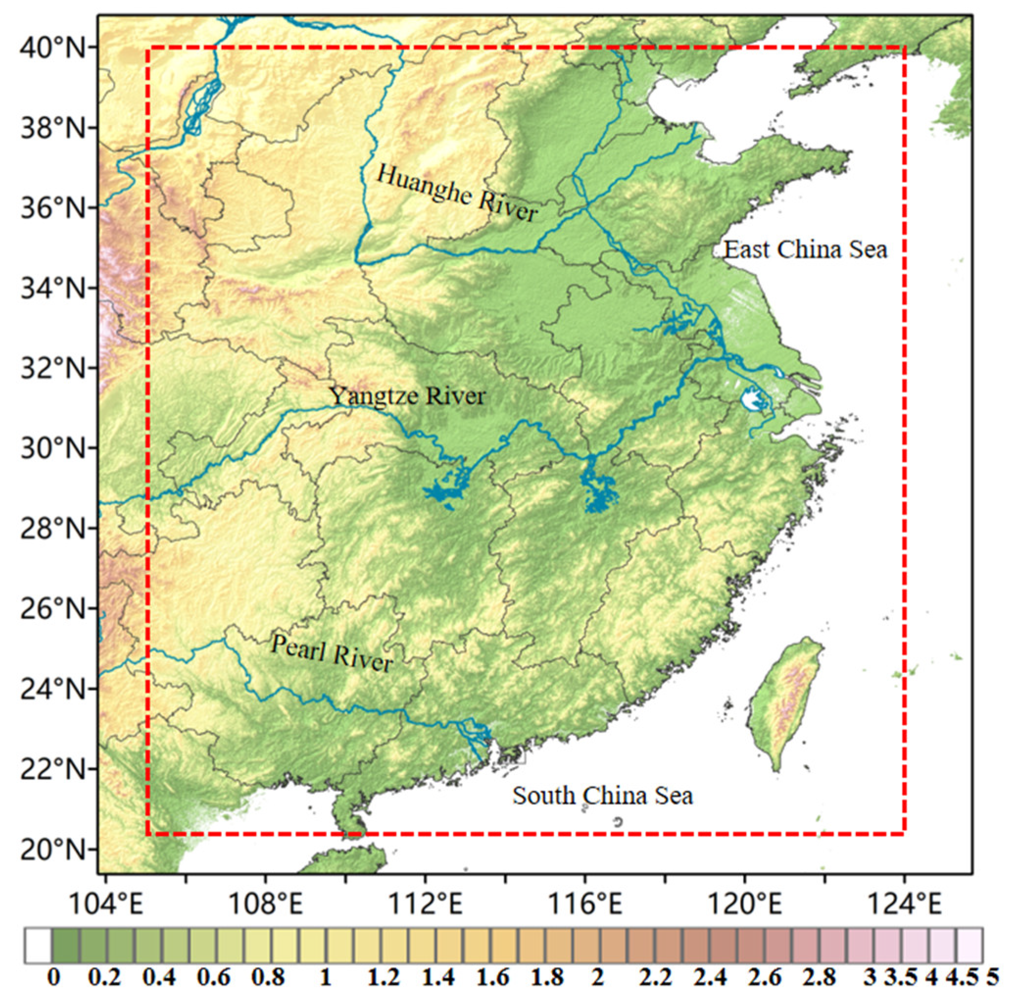
Figure 2.
Histogram and kernel density curve with the ratio of initial area to maximum area for True_CI events (a) and False_CI events (b), magnified by 10 times for True_CI events (a) and False_CI events (b). The blue rectangles represent the frequency distribution histogram. The width of each rectangle corresponds to the value interval of “10 times the ratio of initial area to maximum area”, and the height represents the number of samples falling into that interval; the red smooth curve is the kernel density estimation curve.
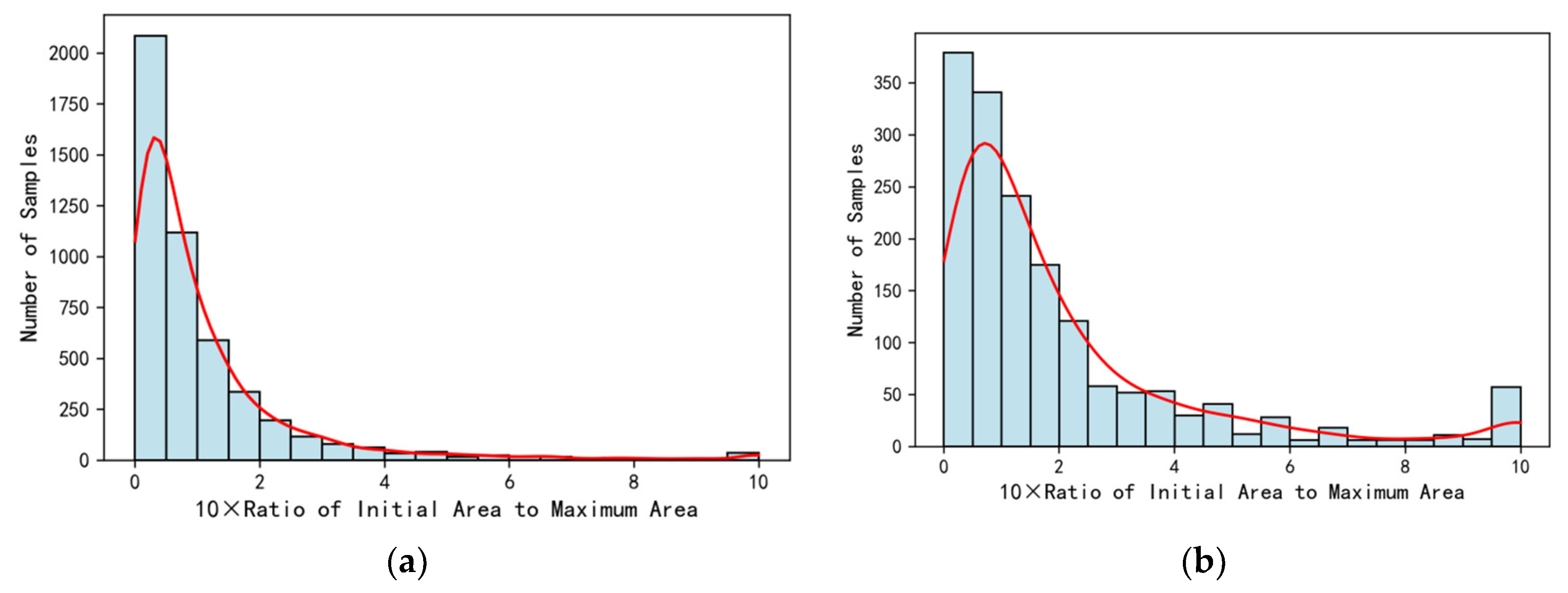
Figure 3.
The comparison and distribution of initial BT versus minimum BT for True_CI events (a) and False_CI events (b). The histogram on the right shows the distribution characteristics of the minimum BT during the process, the histogram at the top shows the distribution characteristics of the initial BT, and the honeycomb scatter distribution reflects the change relationship of samples from the initial BT to the minimum BT during the process.
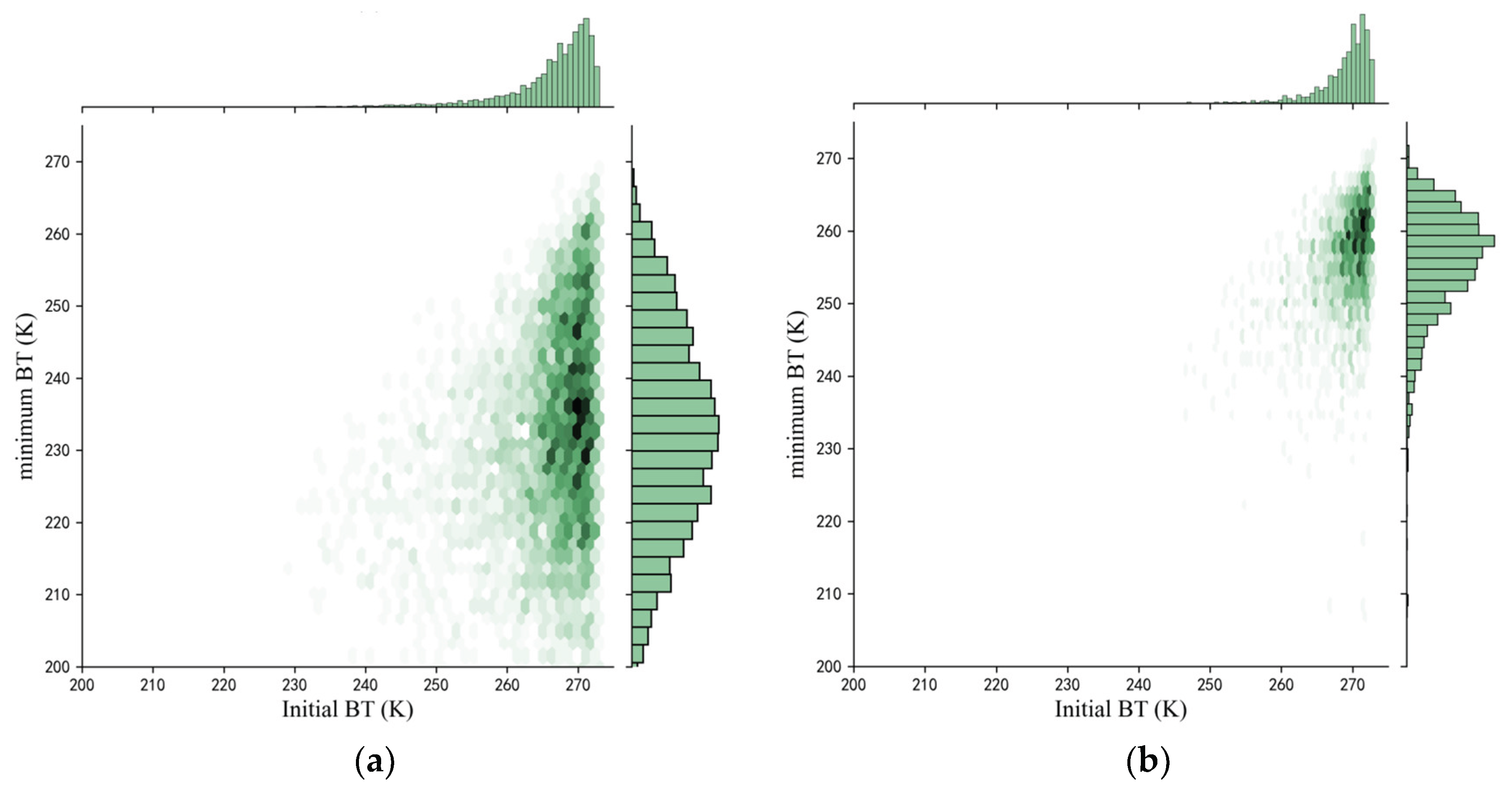
Figure 4.
Images of BT at the 10.7-μm (a, c) and radar composite reflectivity (b, d) on June 10 (a, b) and August 18 (c, d), 2018. The location of CI is marked with a red circle.
Figure 4.
Images of BT at the 10.7-μm (a, c) and radar composite reflectivity (b, d) on June 10 (a, b) and August 18 (c, d), 2018. The location of CI is marked with a red circle.
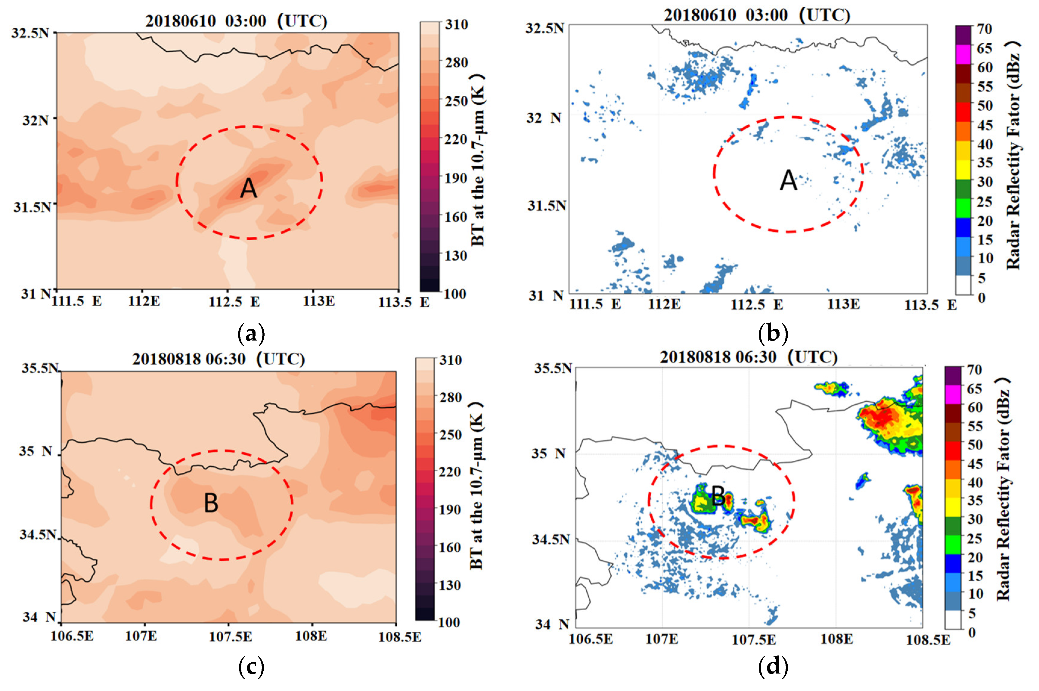
Figure 5.
This Distributions of the 15-min temporal differences of (a) Tb, 10.7, (b) Tb, 7.1-Tb, 10.7, (c) Tb, 12.0-Tb, 10.7, and (d) Tb, 8.5 +Tb, 12.0-2Tb, 10.7 at different times prior to CI occurrence. The orange box is for True_CI events and the bule box is for False_CI events. The box edges indicate the 25th and 75th percentiles, and The line in the middle of the box represents the median value.
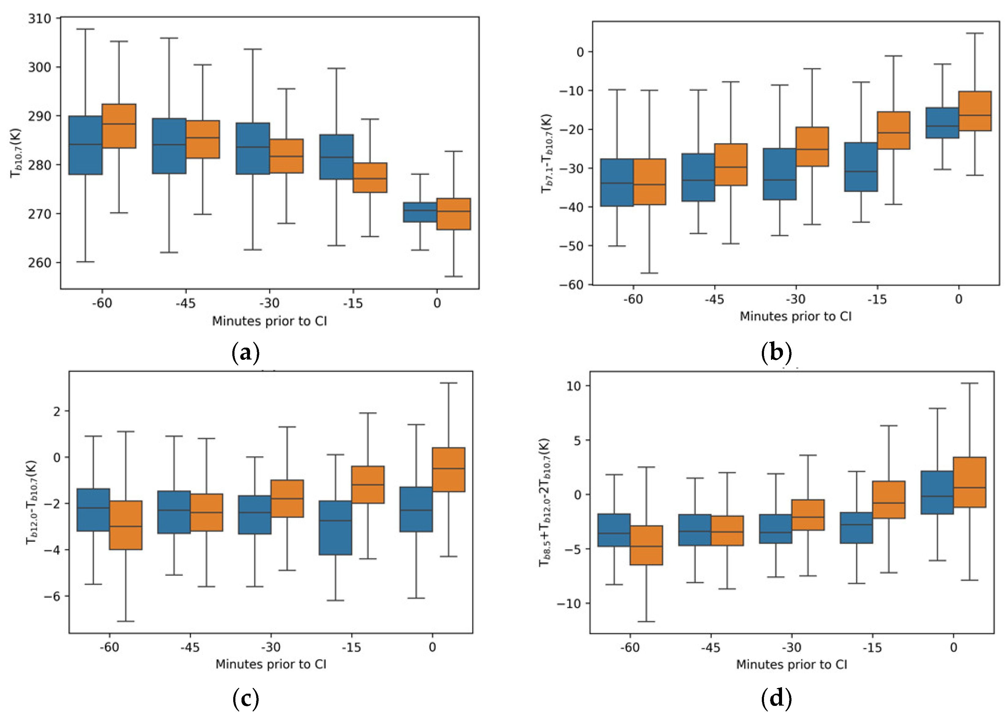
Figure 6.
This Spatial-temporal distribution of the differences between the actual values of three brightness temperature difference metrics of BTD7.1-10.7, BTD12.0-10.7, and BTD8.5 + 12.0 - 2*10.7 for True_CI events at 15 minutes prior to CI and their corresponding reference thresholds. Rows correspond to different latitude ranges (in degrees North), columns correspond to months from April to September, and each cell displays the magnitude of the difference.
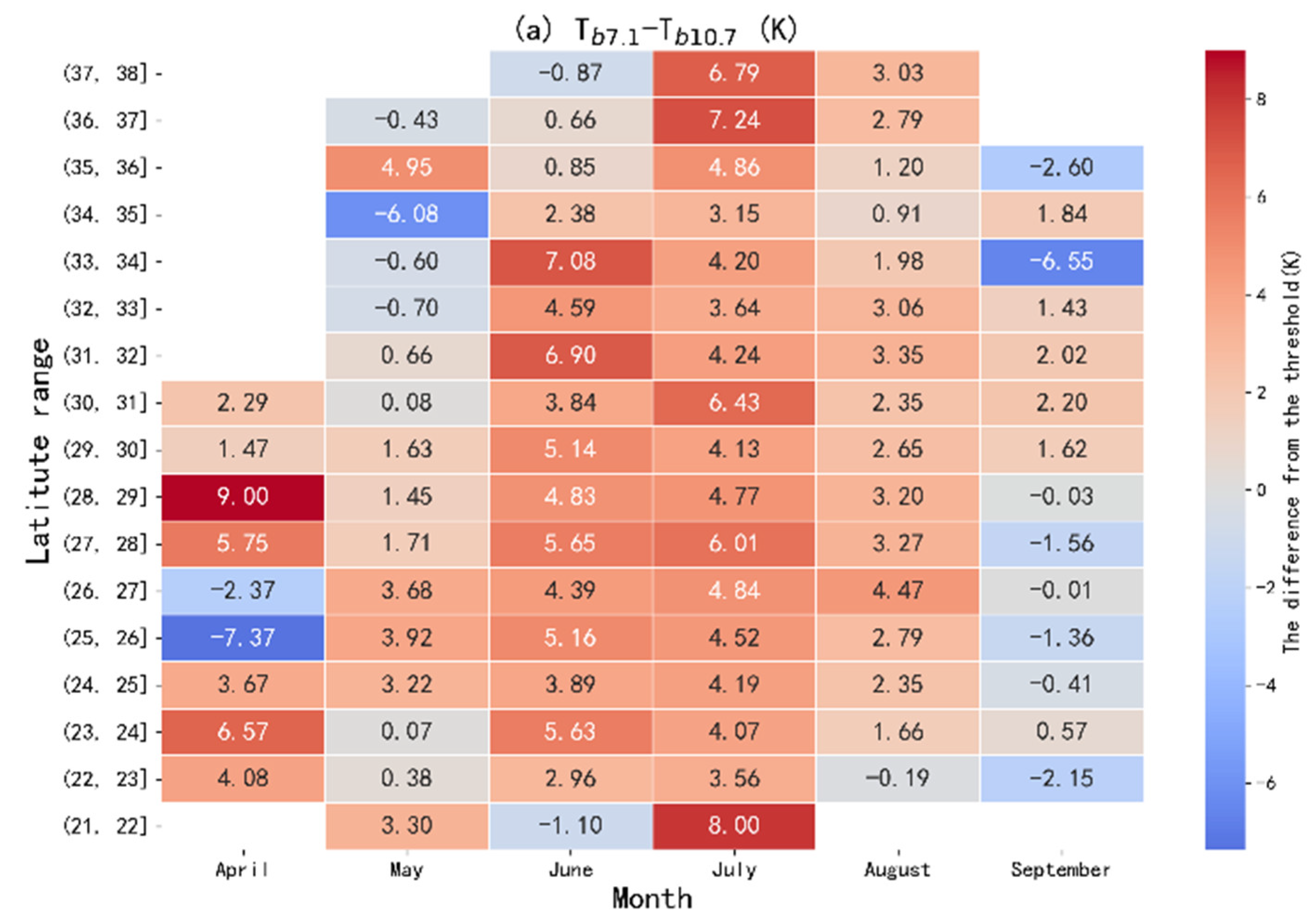
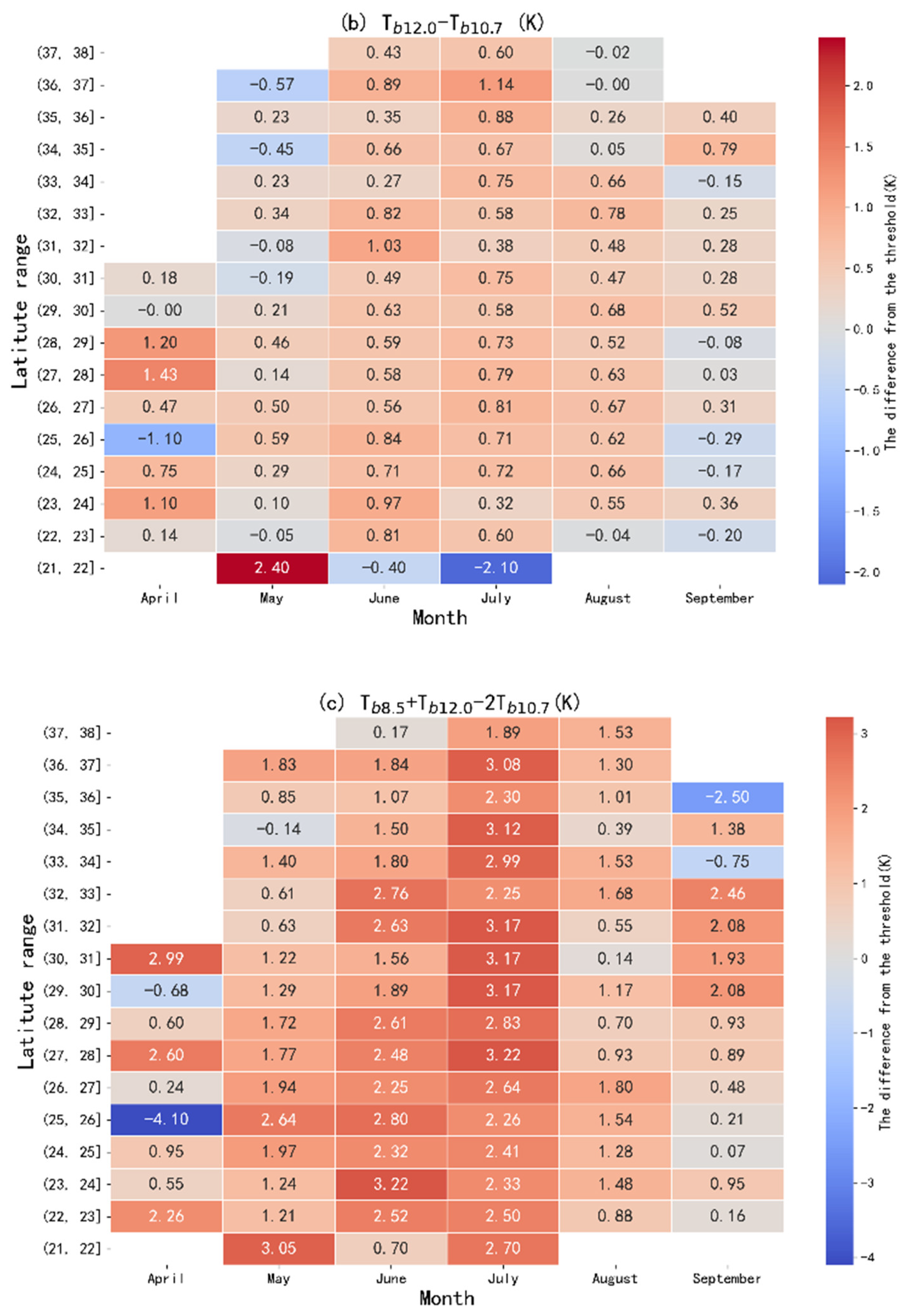
Figure 7.
Time variation of BT at 10.7-μm channel for the missed case and false alarm case. The x-axis represents time relative to the moment of CI occurrence (unit: minutes). Specifically, “0” denotes the moment when CI occurs; negative values represent the time prior to CI occurrence, and positive values indicate time after CI occurrence. The blue line denotes the missed case on 1 July 2018, while the red line denotes the false alarm case on 1 August 2018.
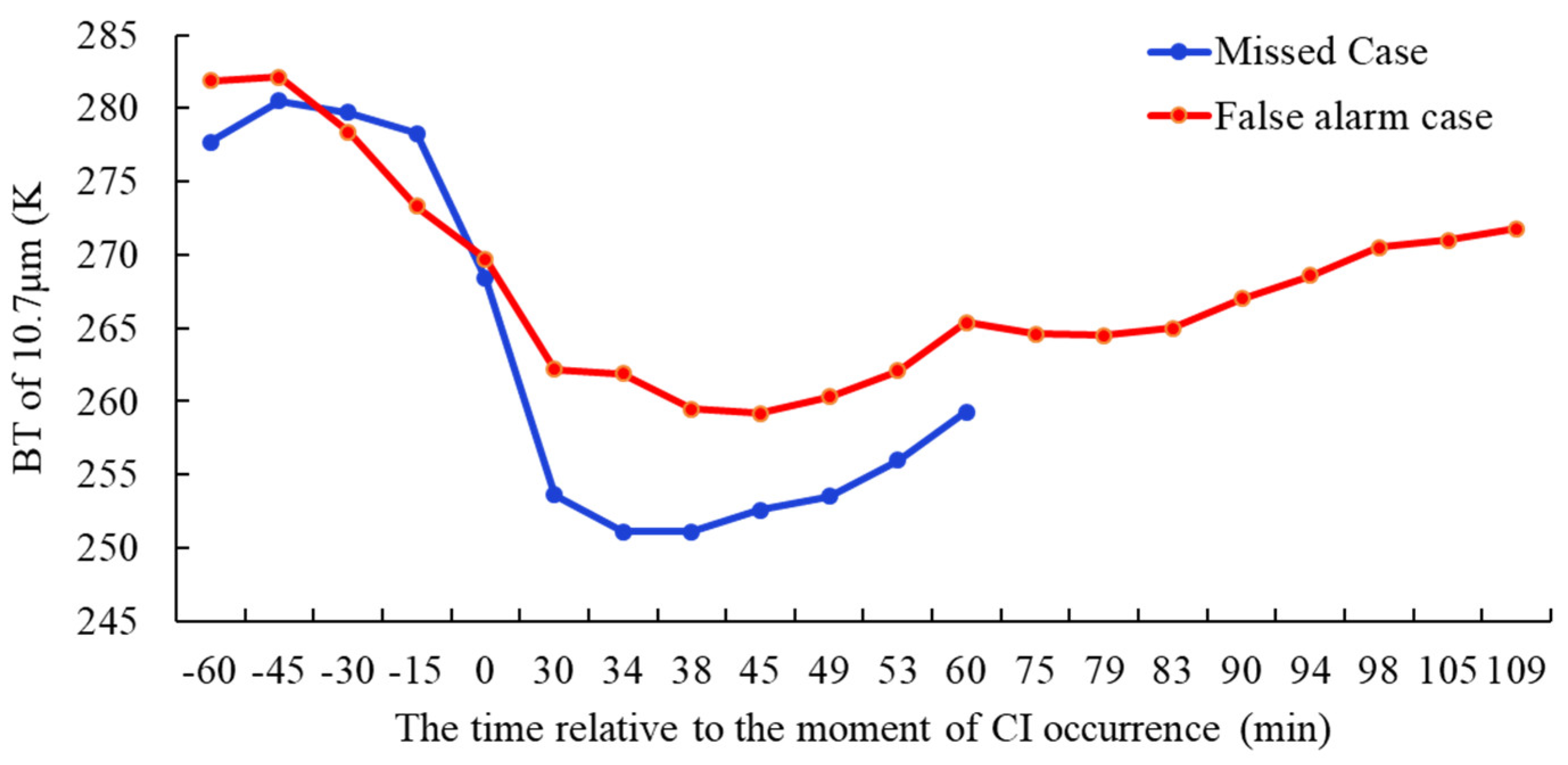

Table 1.
Channel number, wavelengths and description of the channels used in the CI identification algorithm.
Table 1.
Channel number, wavelengths and description of the channels used in the CI identification algorithm.
| Channel name | Spectral range (μm) | Description of main uses |
| 9 | 5.8-6.7 | High-level water vapor |
| 10 | 6.9-7.3 | Middle-layer water vapor |
| 11 | 8.0-9.0 | total water vapor, clouds |
| 12 | 10.3-11.3 | Clouds, surface temperature, etc |
| 13 | 11.5-12.5 | Clouds, total water vapor volume, surface temperature |
| 14 | 13.2-13.8 | Clouds, water vapor |
Table 2.
List of interest fields, along with their definitions and physical relationships to convective clouds.
Table 2.
List of interest fields, along with their definitions and physical relationships to convective clouds.
| Infrared interest fields | Definition | Physical Implications |
| Tb, 10.7 | BT at the 10.7-μm band | Cloud-top height |
| Tb, 7.1-Tb, 10.7 | BT difference between the 7.1-μm band and 10.7-μm band | Cloud-top height relative to lower-troposphere |
| Tb, 12.0-Tb, 10.7 | BT difference between the 10.7-μm band and 12.0-μm band | Cloud optical thickness |
| Tb, 8.5 +Tb, 12.0-2Tb, 10.7 | Tri-channel difference of 8.5-μm band, 12.0-μm band and 10.7-μm band | Cloud-top phrase |
Table 3.
Results identified by the definition method from May to August.
| Month | POD | MAR | FAR |
| May | 79% | 21% | 18% |
| June | 81% | 19% | 0% |
| July | 82% | 18% | 0% |
| August | 84% | 16% | 22% |
Table 4.
Time variations of four indications 1 hour before CI occurrence.
| Time prior to CI occurrence (min) | Tb10.7μm | Tb7.1μm-Tb10.7μm | Tb, 12.0-Tb, 10.7 | T8.5 + 12.0 - 2*10.7 | ||||
| Missed case | False alarm case | Missed case | False alarm case | Missed case | False alarm case | Missed case | False alarm case | |
| -60 | 277.7 | 281.9 | -26.2 | -26.6 | -1.9 | -1 | -2 | -1.4 |
| -45 | 280.5 | 282.1 | -30.4 | -27.4 | -2.5 | -1.9 | -2.8 | -2.6 |
| -30 | 279.7 | 278.4 | -31.4 | -23.5 | -1.7 | -1.1 | -1.3 | -3.7 |
| -15 | 278.3 | 273.3 | -26.2 | -18.7 | -3.1 | -0.8 | -0.5 | -1.9 |
| 0 | 268.4 | 269.7 | -21.6 | -15.5 | -5.1 | 1.1 | -0.5 | 0.8 |
Disclaimer/Publisher’s Note: The statements, opinions and data contained in all publications are solely those of the individual author(s) and contributor(s) and not of MDPI and/or the editor(s). MDPI and/or the editor(s) disclaim responsibility for any injury to people or property resulting from any ideas, methods, instructions or products referred to in the content. |
© 2025 by the authors. Licensee MDPI, Basel, Switzerland. This article is an open access article distributed under the terms and conditions of the Creative Commons Attribution (CC BY) license (http://creativecommons.org/licenses/by/4.0/).
Copyright: This open access article is published under a Creative Commons CC BY 4.0 license, which permit the free download, distribution, and reuse, provided that the author and preprint are cited in any reuse.


