
Submitted:
28 October 2025
Posted:
29 October 2025
You are already at the latest version
Abstract
This methodology investigates the determination of the fracture toughness of 3D-printed specimen, under monotonic loading conditions. The application is based on the use of a Single Edge Notch Bending (SENB) specimen made by a 3D-printing process (stainless-steel 17-4PH). The load-displacement curves exhibited linear behavior until crack initiation, indicating that the Linear Elastic Fracture Mechanics (LEFM) can be used under the small-scale yielding assumption.
The methodology established in the paper represents the major outcome to characterize the fracture toughness of the material. The aim of the paper is twofold. The one is to describe the procedure allowing the identification of the crack initiation through the monitoring of the Crack Mouth Opening Displacement (CMOD), and the second is to determine the critical fracture toughness of the 3D-printed material of the specimen.
Keywords:
additive manufacturing
; fused filament fabrication
; digital image correlation
; fracture toughness
; stress intensity factor
; j-integral
; advanced structured material
1. Introduction
Additive manufacturing, commonly known as 3D printing, has transformed numerous industries by allowing the fabrication of intricate components with a high degree of design flexibility (Gardan 2016). This study explores Atomic Diffusion Additive Manufacturing (ADAM), a metal 3D printing process introduced by Markforged with their Metal X system. ADAM involves three stages: printing a part from a filament of metal powder and plastic binder, debinding to remove the binder, and sintering to fuse the metal particles into a solid, dense part (Galati et Minetola 2019). The innovation of ADAM lies in its ability to produce complex, high-strength metal components without expensive tooling, making it a cost-effective solution for small to medium production runs. This process offers significant advancements in industries like aerospace, automotive, and medical (Jones, J., Vafadar, A., & Hashemi, R. 2023).
Among the materials used, 17-4PH stainless steel is particularly valued for its excellent mechanical properties, and its novel application in material extrusion technology, or Bound Powder Extrusion, as used on the Metal X system. The Metal X process enhances design flexibility while streamlining production, offering a more efficient alternative to traditional additive manufacturing techniques (Alkindi et al. 2021). However, characterizing the fracture toughness of this material when 3D printed remains a challenge. In the last seven years, we tried successively to enhance the failure resistance of 3D printed thermoplastic polymers by fused deposition modeling (Gardan, Makke, et Recho 2018) and to evaluate their fracture toughness by the use of Digital Image Correlation (Lenti et al. 2023).
In this study, we aim to describe a robust fracture toughness-based methodology using a coupling of local DIC close to the crack tip and the fracture mechanics analysis.
In order to estimate the fracture toughness of the material, the crack initiation and the Stress Intensity Factor, or the J-integral, are the two parameters to determine.
We used Digital Image Correlation (DIC) to assess the fracture toughness of 3D-printed 17-4PH stainless steel under monotonic loading. To carry out this investigation, Single Edge Notch Bending (SENB) specimens were employed. The load-displacement responses displayed linearity up to the point of crack initiation, justifying the use of Linear Elastic Fracture Mechanics (LEFM) under the assumption of small-scale yielding for the tested material. The onset of cracking was identified by monitoring the Crack Opening Displacement (COD) between the crack lips.
The displacement field measured by DIC was fitted using Williams’ approach, considering the first five terms. The results demonstrated a high degree of accuracy, when it’s determining the displacement field close the notch tip.
Two procedures were tested to locate the crack initiation at the notch tip: the geometric procedure and the optimization procedure. The optimization procedure proved more effective, enhancing the accuracy of Stress Intensity Factor (SIF) calculations and yielding a critical SIF. Additionally, the critical J-integral was determined using a finite element sub-model of the crack tip vicinity, driven by the DIC-measured displacement field. The path independence of the J-integral was confirmed, with a critical value of J.
Only few test specimens are analyzed, with the aim to describe the chosen procedure to evaluate the fracture toughness. Therefore, more test specimens are needed if the aim was a determination of a precise fracture toughness value of the used material.
This research enhances the understanding of the fracture behavior of the tested 3D printed material (here 17-4PH stainless steel) and aims to optimize manufacturing methods for advanced industrial and research applications using such material.
2. Material and Method
2.1. Specimen Printing Method
Also, this work uses an Additive Manufacturing (AM) process called “Metal X”, recently developed by Markforged Inc. (Campbell et Wohlers 2017), refers to a range of ’indirect’ metal AM, and is based on material extrusion technology. The parts are not produced directly; rather, they’re crafted using metal powders that are bound into a filament and then selectively extruded through a nozzle (Gardan 2016). Markforged has named this method “Atomic Diffusion Additive Manufacturing” (ADAM), which revolves around four fundamental steps: design, printing, de- binding, and sintering. The introduced Metal X process is based on an interesting approach to overcome dimensional inaccuracy and provides enhanced design freedom and simplified solution compared to other AM processes (Alkindi et al. 2021). During the sintering process, as the powder burns away, it enables the creation of intricate enclosed internal structures, resulting in lightweight parts without compromising their strength (Chemkhi et al. 2021).
Additionally, the metal powder is encased in a polymer binder, which is subsequently removed upon completion of the printing process (Galati et Minetola 2019). The polymer removes the inherent toxicity and flammability of powders, making 3D metal printing more accessible and quicker, while also cutting down on manufacturing costs (Gonzalez-Gutierrez et al. 2018).
2.2. Additive Manufacturing Parameters
The Metal X printing system developed by Markforged integrates metal injection molding (MIM) and fused filament fabrication (FFF) technologies into Bound Powder Extrusion (BPE) for its printing processes.
The printing process consists of four fundamental steps: design, followed by printing, debinding, drying, and sintering. Initially, the 3D model is sliced into layers using the slicer program “Eiger” from Markforged solution and the layered model is then sent to the Metal X printer. The specific settings used in the “Eiger” software for manufacturing specimens are outlined in Table 1.
The printing process involves selectively extruding the fused filament through a nozzle to produce the “green” part made of 17-4PH metal (stainless steel) powder bound in a polymer matrix. Martensitic stainless steel filament spools with a diameter of 1.75 mm were utilized for printing specimens.
Then, debinding takes place by immersing this “green” part in a specialized solvent (Opteon SF-79) that dissolves the primary binder, resulting in the “brown” part. After solvent debinding, the part is dried before undergoing thermal debinding using the Sinter-1 unit of the Metal X system to completely remove any remaining binder.
The final step involves sintering the part in a high-temperature horizontal tube furnace of the Sinter-1 unit to melt the metal powders and obtain the “silver” part.
2.3. Specimen Geometry and Mechanical Testing
In this study, Single Edge Notched Bending (SENB) specimens were utilized to assess the fracture toughness of the printed stainless steel. The geometry and dimensions of the samples are illustrated in Figure 1a, with the specimen thickness measuring approximately 10 mm. Two-dimensional digital image correlation (2D-DIC) was employed to capture the displacement and strain fields on the specimen’s surface. To enable this, the printed samples were coated with a random speckle pattern, allowing for precise tracking of surface displacements (see Figure 1b).
Three-point bending tests were conducted using an Instron 4484 tensile testing machine, equipped with custom supports designed to prevent out-of-plane specimen rotation. The crosshead speed was set to 0.5 mm/min, and data acquisition occurred at a rate of 500 measurements per second. A 20 kN load cell was used for force measurements. For each configuration “classical” and “optimized” three specimens were tested. The testing setup was synchronized with a camera capturing one image every two seconds, with a resolution of 1280 × 960 pixels and a scale of 0.04 mm/pixel.
2.4. Digital Image Correlation (DIC)
Digital Image Correlation (DIC) is a technique used to determine the displacement field within a specified Region of Interest (ROI) on a material subjected to deformation. The process involves partitioning the reference image into smaller areas, known as subsets, and tracking their movements in the corresponding deformed image. From the resulting displacement field, the strain field can be calculated by applying spatial differentiation, ensuring that rigid body motions, such as translations and rotations, are properly excluded from the analysis.
In this study, DIC analysis was performed using NCORR software (Blaber, Adair, et Antoniou 2015; Harilal & Ramji 2014). Given the relatively low level of deformation, the initial undistorted image of the sample was used as the reference. Displacement and strain fields were then calculated relative to this reference. The ROI was strategically placed away from the image borders to ensure it remained within the field of view after deformation.
For the analysis, the subset size was chosen to be larger than the filament width to ensure a homogenized displacement value. Specifically, a subset radius of 30 pixels was selected, with a grid spacing of 4 pixels. This configuration resulted in approximately 90% overlap between adjacent subsets, ensuring smoothness in the resulting displacement field. Subset truncation was also applied, as illustrated in Figure 2.
Accurate strain determination is a critical aspect of DIC, as it requires differentiation of the displacement field, a process that is sensitive to noise. To mitigate this, the displacement gradient is computed using the strain window method (Pan et al., 2007). The displacement components, denoted as U(X, Y) and V(X, Y) over a given range (Xmin < X < Xmax and Ymin < Y < Ymax), were fitted to a plane equation using least squares curve fitting. The user has the option to adjust the window size (both in the X and Y directions) for optimal accuracy.
The Green-Lagrange strain has been computed by using the resulting plane slopes as follows:
Table Green-Lagrange strain has been computed by using the resulting plane slopes as follows:
3. Load Displacement Curves
Figure 3 shows load-displacement curve of the sample is presented, revealing two distinct stages in the ascending portion of the graph. The first regime is for displacement d < 0.15 mm. It is characterized by a low stiffness due to setting the test. The second one is for d > 0.2 mm, where the curve becomes perfectly linear. The slope of this part is equal to 12.16 kN.mm-1. At the end of the rising branch the force reaches 8.4 KN, after that, it drops down. This behavior corresponds to the crack initiation and growth in the sample. It is worth noting that the sample behavior is almost linear until the crack initiation. There is apparent plasticity signature observed during the loading prior to the crack initiation. Therefore, Linear elastic fracture mechanics assumption is relevant in such a case. Moreover, Finite element simulation of the SENB deformation has been performed to calibrate the Young’s modulus of the sample. The results shows that Young’s modulus of 150 GPa leads to a sample stiffness consistent with the one calculated from the experimental results.
4. Detection of Crack Initiation by DIC
To determine the critical Stress Intensity Factor of the specimen, it is essential to precisely identify the moment when crack initiation occurs. In SENB specimens, crack propagation begins with the upward movement of the singularity tip. This alters the displacement field near the notch tip, thereby affecting the Crack Mouth Opening Displacement (CMOD).
Figure 4 shows the evolution of the crack tips mouth opening displacement during the sample deformation. It’s plot with respect to the snapshot number n which is proportional to the applied displacement so that:
where is the loading velocity and δt is time window between two subsequent snapshots.
The curve exhibits two distinct regimes, separated by a sharp increase in the Crack Mouth Opening Displacement (CMOD). In the initial regime, where n<100, the CMOD increases linearly with the applied load, reflecting the elastic behavior of the material as it deforms without any significant crack growth. During this phase, the sample responds elastically, and the deformation remains relatively uniform across the material. In contrast, for n>110 the CMOD continues to increase linearly with the applied load, but with a steeper slope, indicating the onset of crack propagation within the sample. This steeper slope reflects the material’s transition from elastic behavior to the irreversible process of crack growth, where the displacement becomes more pronounced as the crack propagates further. The sharp transition between these two regimes signals the initiation of crack growth, with the inflection point at n=105 being considered the threshold where the crack begins to propagate. This value was determined by calculating the average within the transition region, providing a reliable estimate for the point at which crack growth is triggered.
5. Fracture Toughness Characterization Results
5.1. Determination of the Stress Intensity Factor SIF
The evaluation of the critical Stress Intensity Factor (SIF) involves analyzing the displacement field within a circular Region of Interest (ROI) centered at the notch tip. This displacement field is obtained through Digital Image Correlation (DIC) for each captured image throughout the deformation process. The connection between the SIF and the displacement field near the notch tip is described by the Williams analytical solution.
For SENB sample submitted to mode I loading condition (see Figure 5), the stress field around the V-notch tip can be written as follow (Williams 1952):
where is the mode I eigenvalues. re the root of the following equation:.
where and is the V-notch tip angle. Only the root with a positive real part can be accepted. Equation (6) has been solved numerically. Table 2 shows the values of the first five . As < 1 thus the first stress term in Equation (5) is singular with a singularity degree of (1 −). Therefore, the Notch Stress Intensity Factor NSIF, in this case, can be written as:
where A1 is the first term in the stress Equation (5). To determine the coefficients Ai, the displacement field around the notch tip is used. The displacement field can be expressed as:
where µ is the shear modulus and κ is the Kolosov’s constant.
The Equation (7) shows the dependence of SIF with the singularity degree that depends upon the V-notch angle. The measured displacement field has been employed to fit the coefficients of the William’s solution through a numeric method as detailed in Appendix A. The eigenvalues are the roots of Equation (6). The first 5 terms are only considered in Equations (8) and (9).
Figure 6a compares the displacement field measured by DIC (dots) and the one fit by William’s solution (mesh). The displacement field normal to the crack surface is shown in this case. Figure 6b presents a scatter plot of the fitted displacement values versus those measured by DIC, where each point corresponds to a subset. The color of each point reflects its distance from the crack tip. The alignment of the data along the first bisector indicates a strong agreement between the measured and modeled displacement fields. All points are within a scatter band of ±0.01, however, the points deviate from the first bisector as it becomes closer to the notch tip. This is somewhere related to the decrease of the accuracy of the DIC when a subset is close to the tip as shown by the correlation coefficient of the subsets shown in Figure 6.
5.2. Accurate Detection of the Crack Tip Position
The William solution gives the displacement field with respect to the polar coordinate of a point taking the tip as the origin of the reference. Thus, the identification of the tip is critical to convert the subset position from cartesian to polar coordinate system. Any shift of the tip position can reduce drastically the precision of the fit. To identify the tip position two methods were tested:
- -
- geometrical method: where the tip position is identified by the contrast of pixel color at the boundary of the V-Notch.
- -
- optimization method: where the tip is searched within a square of 15×15 pixels centered by the expected geometric notch tip. Each pixel is considered as a potential notch tip. Thus, the polar coordinates of each subset were calculated. The measured displacement field fits with William’s equation. Then a residual is calculated. The pixel that leads to a minimum residual is the one that is considered as the crack tip.
Figure 7 shows the scatter plot between the fitted and the measured displacement field for both methods. Both scatters show a good correlation, however, the scatter width is larger if the tip is determined by geometric method. These results depict that accurate identification of notch or crack tip can be done by using the optimization method. The displacement field of the snapshot that corresponds to the onset of the crack was used to determine the critical SIF K∗. The result shows that .
5.3. J Integral Evaluation
In the case of LEFM assumption the J integral represent the energy release rate of the crack extension. It’s given by the following equation:
where is the strain energy density. is the traction vector. is the displacement vector. is the contour around the crack tip.
As shown by the Equation (11) the J integral calculation requires the stress which cannot be measured. The only information accessible by DIC is the displacement field and its gradient. To circumvent this issue, a method based on the submodeling of the crack tip by finite element is suggested. Figure 8 describes the sequence of steps of this method. It can be summarized as follow:
- -
- Considering the ROI used in DIC, the grid of the subsets is converted to finite element mesh.
- -
- In each element the displacement measured by DIC can be written and the same for where Ni(x, y) are the shape functions of quadrangle elements.
- -
- In the other side, a finite element submodel that encircle the is defined. The contour of this submodel is driven by the displacement measured by DIC.
- -
- The J integral is calculated from the FE solution.
The J-integral was calculated for different circular contours with various radii. Figure 9 shows the J integral value with respect to the contour radius. The result depicts that J-integral becomes path independent for contour radius between 3 mm to 8 mm. For < 3 mm the contour is close to the tip while for > 8mm the contour is close to the boundary layer where the driven displacement is applied. The crtical J integral found is . For plain stress assumption we check that the value of verify the equation
6. Conclusions
Digital image correlation has been employed to characterize the fracture toughness of 3D-printed material (here stainless- steel 17-4PH) following a methodology based on the use of SENB specimens which are submitted to three points bending test.
The load- displacement curve of the sample shows that the behavior is still linear till the crack initiation. This behavior reveals that the use LEFM with small scale yielding assumption is justified for this type of material. The load displacement curve is used to calibrate the Young’ modulus and E=150 GPa is found.
The snapshot that corresponds to the crack initiation in each sample has been identified using the Crack Mouth Opening Displacement CMOD.
The displacement field of this sample was fit by William’s equation taking into consideration the first five terms of the equation. The results show that William’s equations fit the displacement field accurately with a determination coefficient close to one for all cases. This also justifies the use of LEFM assumption.
To identify the position notch tip, two methods were tested in order to guarantee a reliable result: the geometrical method and the optimization method. The results highlight an improvement of the accuracy of SIF calculation when the optimization method is used. The critical SIF found is Otherwise, the geometrical method is easier to use and provides almost good result.
Finally, the critical J integral J∗ of the sample has determined using a finite element sub-model at the crack tip vicinity. The sub-model deformation was driven by the displacement field measured by DIC. The path independence of J integral was verified. The critical value of J integral found is It’s to be noted that -integral determination represents a verification to the - Stress Intensity Factor calculation.
Appendix A. Determination of the Coefficients AI
Equations (8) and (9) show that the displacement field results from the summation of several terms. The first term A1 is used in the evaluation of the NSIF. The higher-order terms (n ≥ 2) have to be taken into account to fit accurately the displacement field around the notch. In this context, several studies (Yates, Zanganeh, et Tai 2010; Torabi, Bahrami, et Ayatollahi 2019; Bahrami, Ayatollahi, et Torabi 2020; Miarka et al. 2020) showed that at least 5 terms are required to converge to a stable value of NSIF. In the following, only the first five terms are considered.
The Equations (8) and (9) can be written in a simple matrix equation form as follows:
where
And
and are the polar coordinates of the subset. 1 ≤ i ≤ m, m is the total number of the subset in the ROI.
Conversely, the SENB specimens exhibit significant Rigid Body (RB) displacement at the notch tip due to central bending. As a result, it is necessary to account for the RB contribution within the measured displacement field. To incorporate these effects, translation and rotation terms representing rigid body motion are added to Equation (14), which is then modified accordingly:
is the translation vector and R is the magnitude of RB rotation. The matrix form shown in Equation (15) is more compatible with numerical treatment. In the following, only the displacement component concerning the notch opening is used. To determine the unknown terms: in Equation (15), a non-linear least square method has been employed to fit the measured displacement field around the notch tip. (implemented in Gnuplot (Janert 2016)).
Nomenclature
| ADAM | Atomic Diffusion Additive Manufacturing |
| DIC | Digital Image Correlation |
| LEFM | Linear Elastic Fracture Mechanics |
| SIF | Stress Intensity Factor |
| J-integral | Path-independent integral used in fracture mechanics |
| K_IC | Fracture toughness (critical stress intensity factor) |
| σ | Applied stress (MPa) |
| ε | Strain |
| a | Crack length (mm) |
| E | Young’s modulus (GPa) |
| ν | Poisson’s ratio |
| FEM | Finite Element Method |
References
- Alkindi, Tawaddod, Mozah Alyammahi, Rahmat Agung Susantyoko, et Saleh Atatreh. 2021. « The Effect of Varying Specimens’ Printing Angles to the Bed Surface on the Tensile Strength of 3D-Printed 17-4PH Stainless-Steels via Metal FFF Additive Manufacturing ». MRS Communications 11 (3): 310--16. [CrossRef]
- Bahrami, B., M. R. Ayatollahi, et A. R. Torabi. 2020. « Application of digital image correlation method for determination of mixed mode stress intensity factors in sharp notches ». Optics and Lasers in Engineering 124:105830.
- Blaber, J., B. Adair, et A. Antoniou. 2015. « Ncorr: Open-Source 2D Digital Image Correlation Matlab Software ». Experimental Mechanics 55 (6): 1105--22. [CrossRef]
- Campbell, Ian, et Terry Wohlers. 2017. « Markforged: Taking a different approach to metal Additive Manufacturing ». https://repository.lboro.ac.uk/articles/Markforged_Taking_a_different_approach_to_metal_Additive_Manufacturing/9346493/files/16955546.pdf.
- Chemkhi, Mahdi, J. Marae Djouda, M. A. Bouaziz, J. Kauffmann, F. Hild, et Delphine Retraint. 2021. « Effects of mechanical post-treatments on additive manufactured 17-4PH stainless steel produced by bound powder extrusion ». Procedia CIRP 104:957--61.
- Galati, Manuela, et Paolo Minetola. 2019. « Analysis of density, roughness, and accuracy of the atomic diffusion additive manufacturing (ADAM) process for metal parts ». Materials 12 (24): 4122.
- Gardan, Julien. 2016. « Additive Manufacturing Technologies: State of the Art and Trends ». International Journal of Production Research 54 (10): 3118--32. [CrossRef]
- Gardan, Julien, Ali Makke, et Naman Recho. 2018. « Improving the Fracture Toughness of 3D Printed Thermoplastic Polymers by Fused Deposition Modeling ». International Journal of Fracture 210 (1--2): 1--15. [CrossRef]
- Gonzalez-Gutierrez, Joamin, Santiago Cano, Stephan Schuschnigg, Christian Kukla, Janak Sapkota, et Clemens Holzer. 2018. « Additive manufacturing of metallic and ceramic components by the material extrusion of highly-filled polymers: A review and future perspectives ». Materials 11 (5): 840.
- Harilal, R., et M. Ramji. 2014. « Adaptation of open source 2D DIC software Ncorr for solid mechanics applications ». In 9th international symposium on advanced science and technology in experimental mechanics. Vol. 1. The Japanese Society for Experimental Mechanics.
- Janert, Philipp K. 2016. Gnuplot in action: understanding data with graphs. Simon and Schuster. https://books.google.com/books?hl=fr&lr=&id=RTozEAAAQBAJ&oi=fnd&pg=PT17&dq=Gnuplot+5.2:+an+interactive+plotting+program&ots=7Vg_I8bwXX&sig=yf4un48yKtv1ZDc45dMr4EXxRzs.
- Jones, J., Vafadar, A., & Hashemi, R. (2023). A Review of the Mechanical Properties of 17-4PH Stainless Steel Produced by Bound Powder Extrusion. Journal of Manufacturing and Materials Processing, 7(5), 162. [CrossRef]
- Lenti, Adriano, Ali Makke, Julien Gardan, et Naman Recho. 2023. « Fracture Toughness Characterization of 3D-Printed Advanced Structured Specimens by Digital Image Correlation ». International Journal of Fracture 240 (1): 17--28. [CrossRef]
- Miarka, Petr, Alejandro S. Cruces, Stanislav Seitl, Lucie Malikova, et Pablo Lopez-Crespo. 2020. « Evaluation of the SIF and T-stress values of the Brazilian disc with a central notch by hybrid method ». International Journal of Fatigue 135:105562.
- Pan, Bing, Huimin Xie, Zhiqing Guo, et Tao Hua. 2007. « Full-field strain measurement using a two-dimensional Savitzky-Golay digital differentiator in digital image correlation ». Optical Engineering 46 (3): 033601--033601.
- Torabi, A. R., B. Bahrami, et M. R. Ayatollahi. 2019. « Experimental determination of the notch stress intensity factor for sharp V-notched specimens by using the digital image correlation method ». Theoretical and Applied Fracture Mechanics 103:102244.
- Williams, Max L. 1952. « Stress singularities resulting from various boundary conditions in angular corners of plates in extension ». https://asmedigitalcollection.asme.org/appliedmechanics/article-abstract/19/4/526/1106855.
- Yates, J. R., M. Zanganeh, et Y. H. Tai. 2010. « Quantifying crack tip displacement fields with DIC ». Engineering Fracture Mechanics 77 (11): 2063--76.
Figure 1.
(a) geometry of the Single Edge Notched Bent SENB specimen used in this work. The specimen was printed by FDP. (b) Close up view on the notch region showing the painting pattern used for DIC. The local reference (x, y) and the global one (X, Y) are also shown in this figure. (r, θ) are the polar coordinates of a subset.
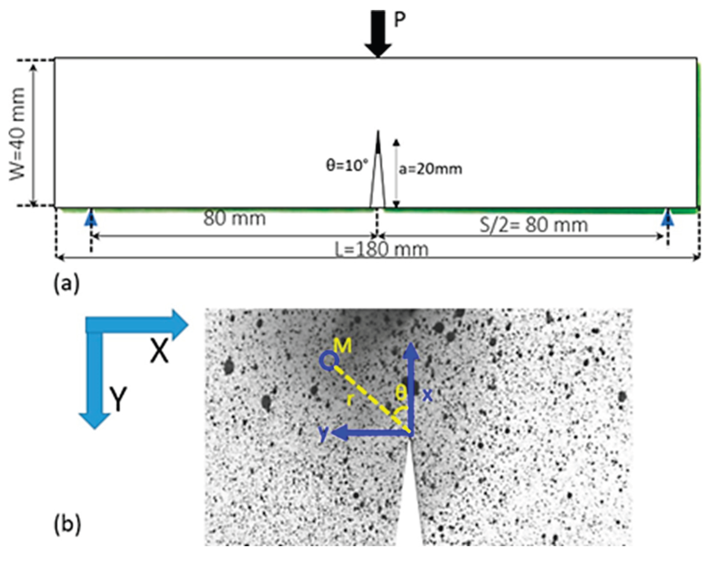
Figure 2.
(a) The local reference at the crack tip close to the V notch, (b) The region of interest taken around the notch. The white circle shows a subset form the ROI. (c) shows the grid of the subset propagation in the ROI.
Figure 2.
(a) The local reference at the crack tip close to the V notch, (b) The region of interest taken around the notch. The white circle shows a subset form the ROI. (c) shows the grid of the subset propagation in the ROI.
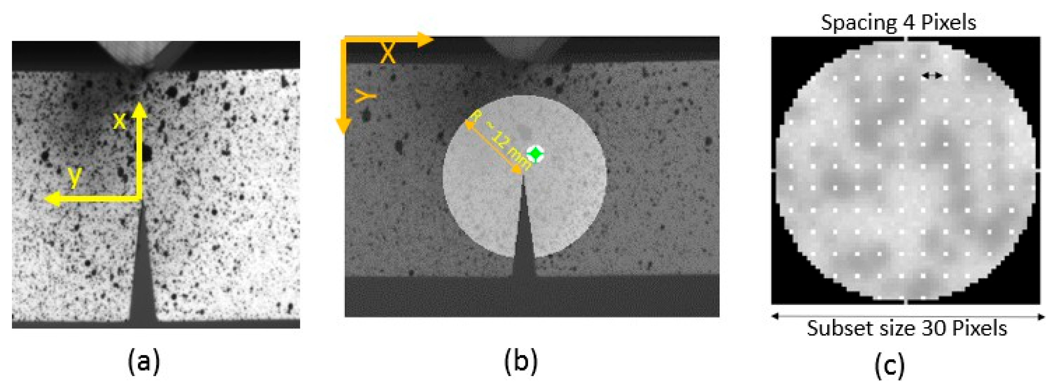
Figure 3.
Load displacement curve.
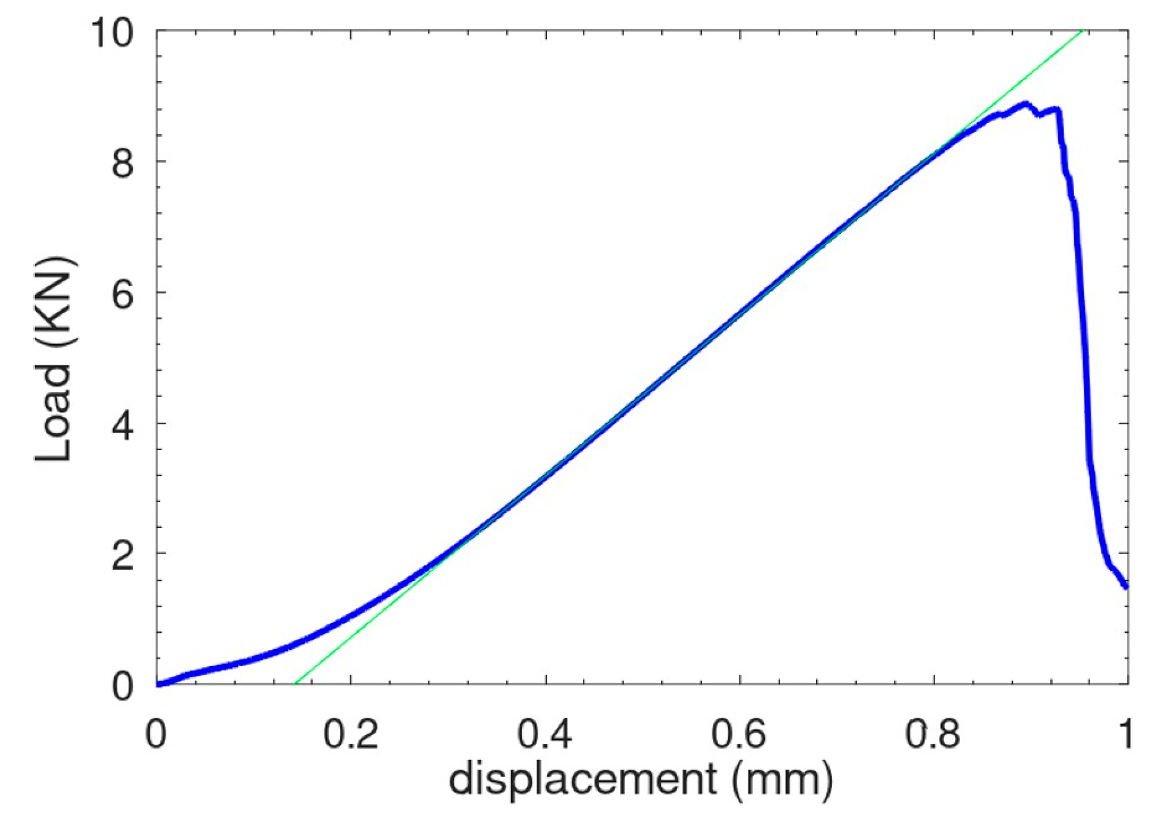
Figure 4.
Crack Mouth Opening Displacement CMOD with respect to the snapshot number during the test. The CMOD is evaluated from two distinct ROIs located beside the main notch as shown in the inset. The sharp increase of the CMOD corresponds to the crack initiation.
Figure 4.
Crack Mouth Opening Displacement CMOD with respect to the snapshot number during the test. The CMOD is evaluated from two distinct ROIs located beside the main notch as shown in the inset. The sharp increase of the CMOD corresponds to the crack initiation.
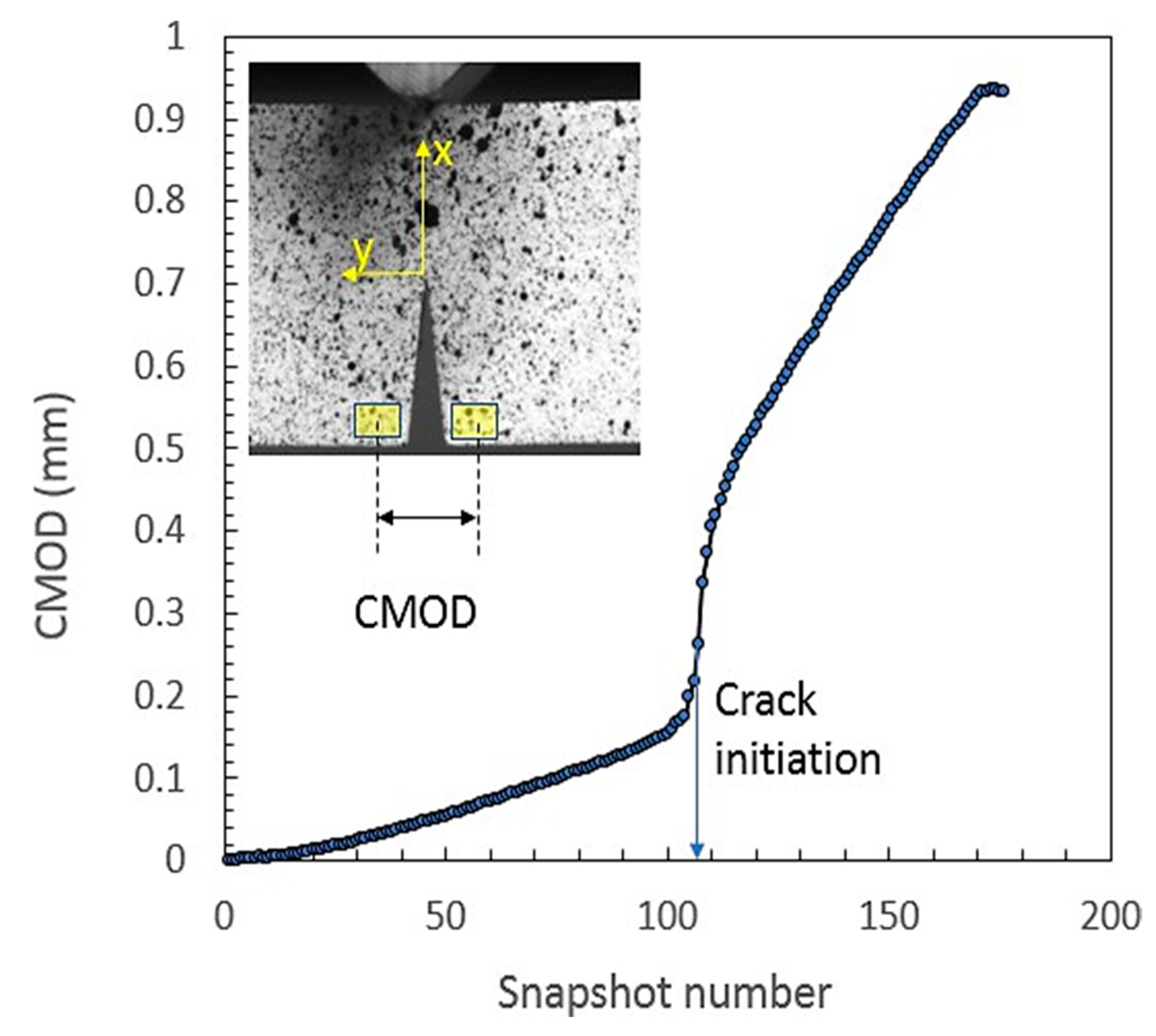
Figure 5.
SENB geometry. Bottom: V notch vicinity with local and global references.
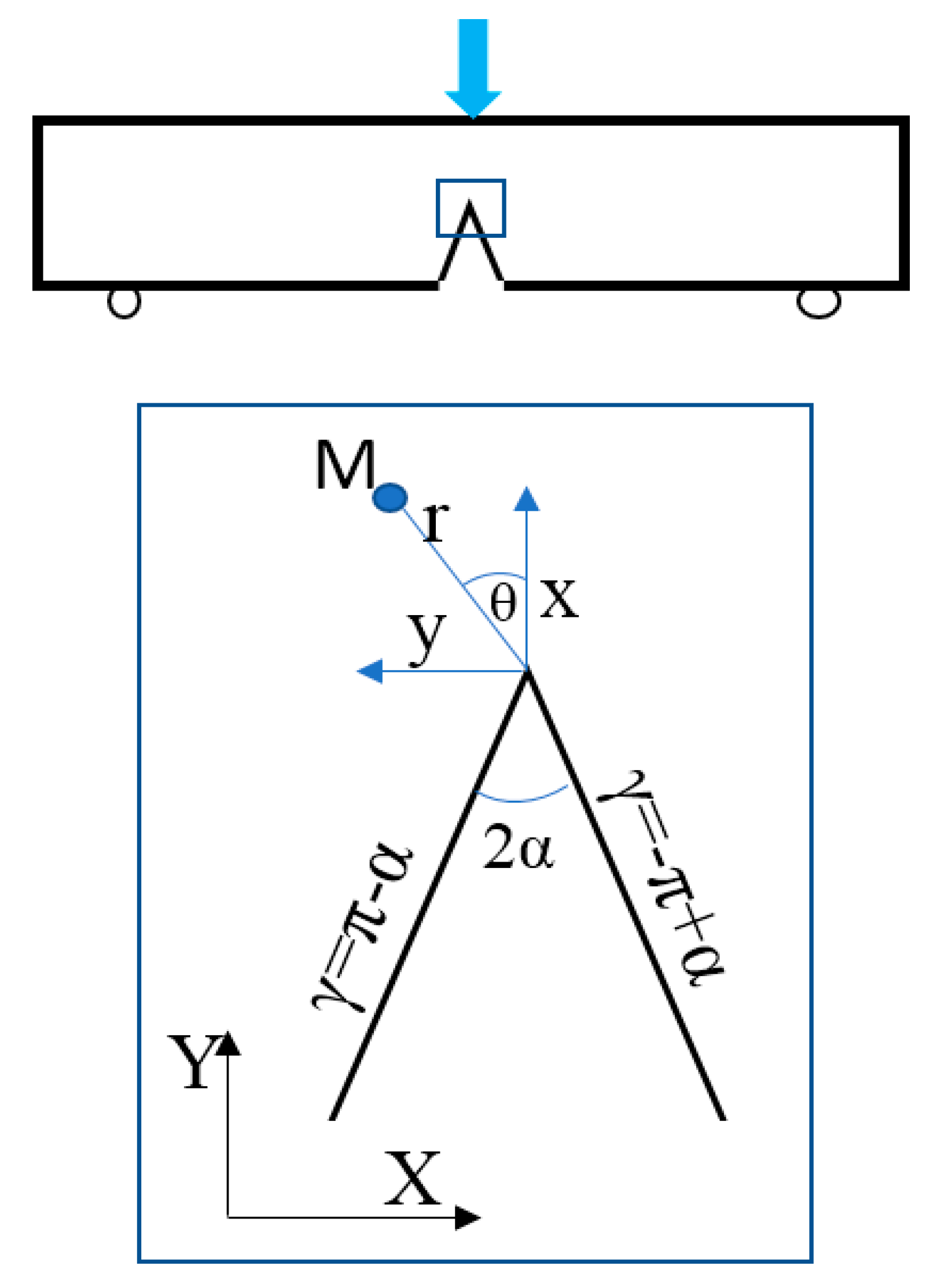
Figure 6.
(a) comparison between the measured and the fit function of the displacement field . (b) scatter plots show the fit value with respect to the measured ones. The points were fitted using a linear function. The slope of this line is the coefficient of determination of the fit. The correlation coefficient for both cases is close to one, which indicates that the fit and measured values are strongly consistent. Moreover, most of the points are within a scatter band of ±0.01mm.
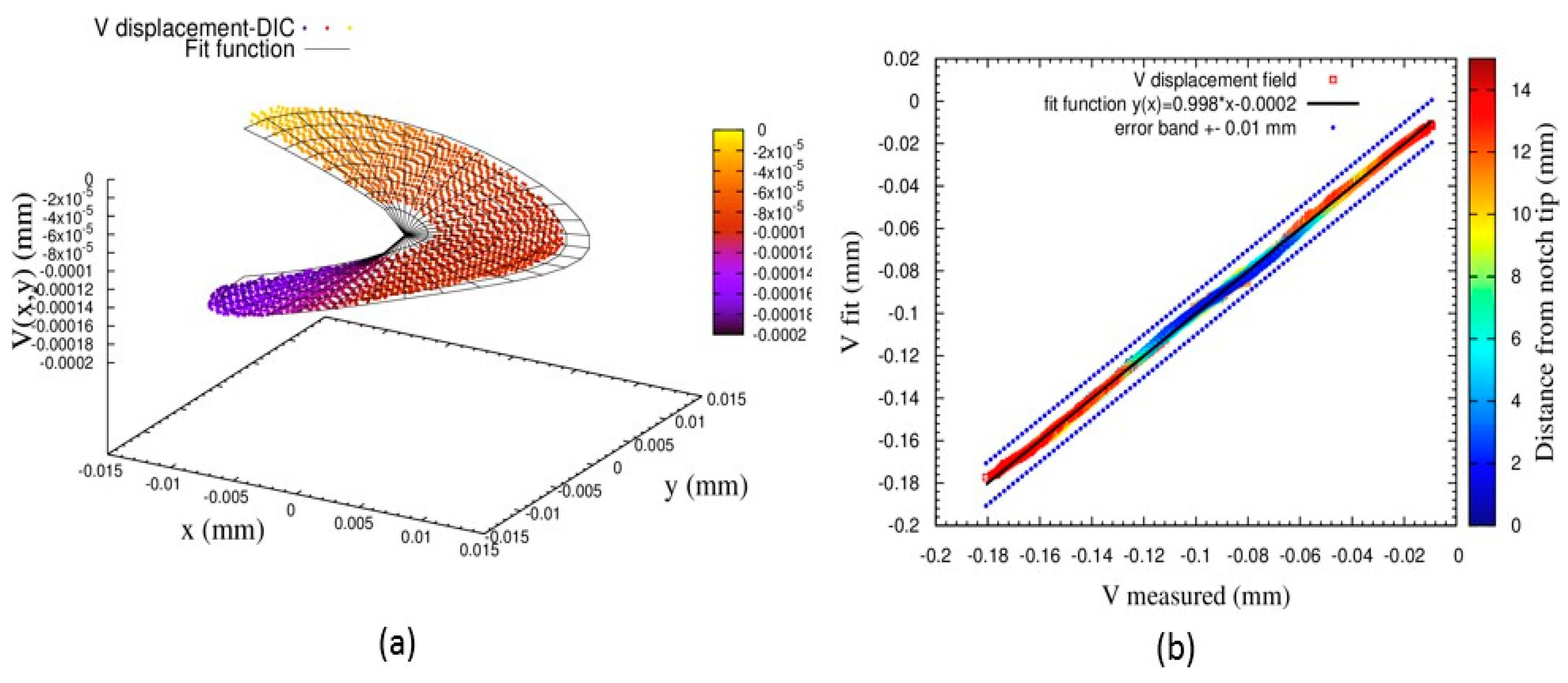
Figure 7.
(a) Scatter plot of the fitted versus the measured displacement field the notch tip is taken as the pixel at the peak of the notch as depicted in the inset. (b) same curve as in (a) but the crack tip is taken as the pixel that minimizes the residual .This pixel is searched within a window of 15 × 15 pix around the geometric crack tip as shown in the inset.
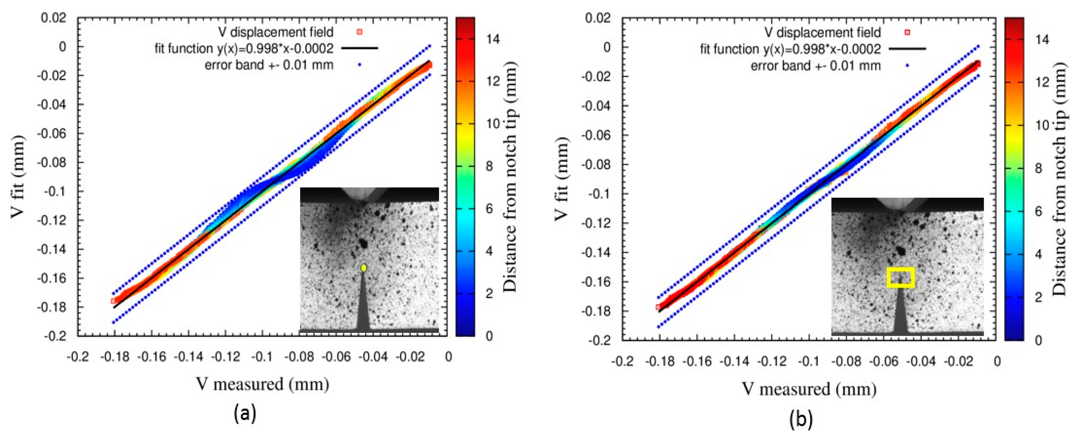
Figure 8.
Description of the process used to compute J integral. Starting from the displacement field determined by DIC, the grid of subsets center is converted to finite element mesh. Quadratic shape functions are used to interpolate the displacement field. This field is used to drive the deformation of a local finite element submodel. The obtained stress, strain, and the displacement fields are used to compute J-integral.
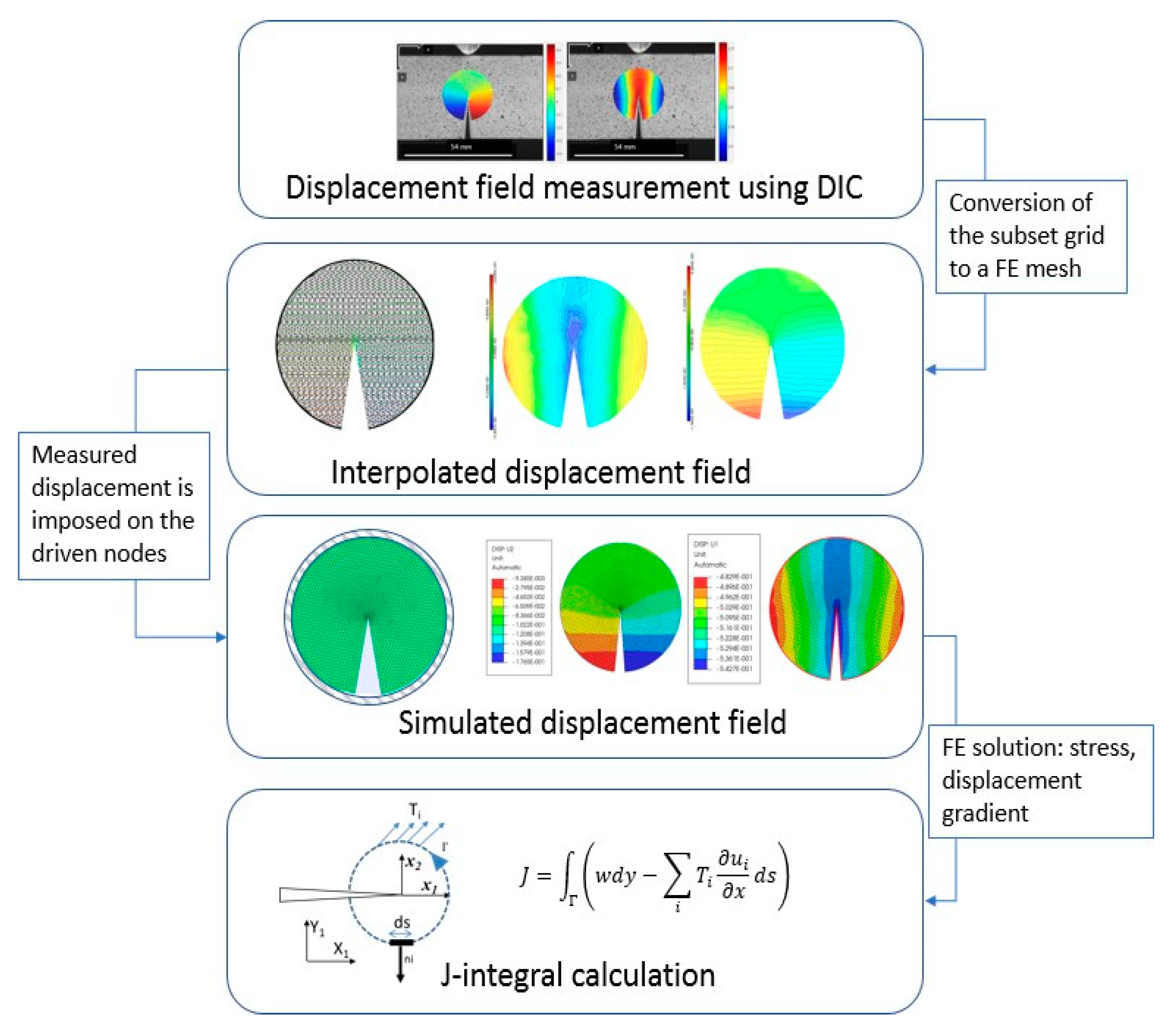
Figure 9.
J-integral computed at different circular contours with various radius. The inset shows the domain where computing j-integral is reliable.
Figure 9.
J-integral computed at different circular contours with various radius. The inset shows the domain where computing j-integral is reliable.
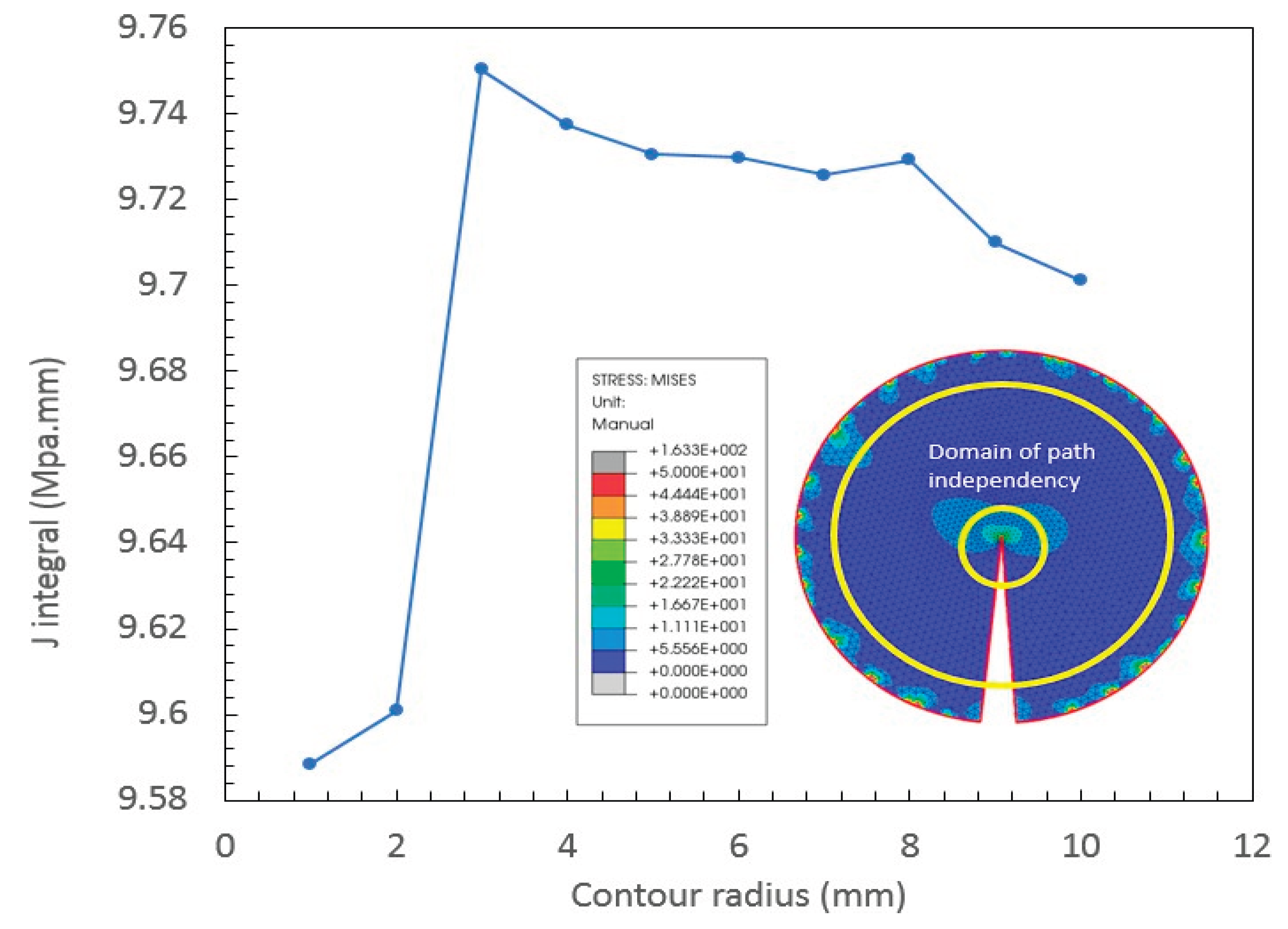

Table 1.
AM processing parameters for manufactured specimens.
| Metal X Processing parameters | As fabricated |
| Samples Filament material | 17-4PH stainless steel |
| Furnace type | Sinter-1 |
| Infill pattern | Triangular fill |
| Post-Sintered Layer Height (µm) | 125 |
| Wall layers (contours) | 4 walls (1mm post sintered) |
| Roof and floor layers (top and bottom) | 4 layers (0.50mm post-sintered) |
| Use Raft | Yes |
| Sinter Stability | Yes |
Table 2.
The first five values of calculated for V-notch tip angle 2α = 10 deg.
| 0.5001 | 1.0588 | 1.4997 | 2.1188 | 3.1815 |
Disclaimer/Publisher’s Note: The statements, opinions and data contained in all publications are solely those of the individual author(s) and contributor(s) and not of MDPI and/or the editor(s). MDPI and/or the editor(s) disclaim responsibility for any injury to people or property resulting from any ideas, methods, instructions or products referred to in the content. |
© 2025 by the authors. Licensee MDPI, Basel, Switzerland. This article is an open access article distributed under the terms and conditions of the Creative Commons Attribution (CC BY) license (http://creativecommons.org/licenses/by/4.0/).
Copyright: This open access article is published under a Creative Commons CC BY 4.0 license, which permit the free download, distribution, and reuse, provided that the author and preprint are cited in any reuse.


