
Submitted:
26 October 2025
Posted:
27 October 2025
You are already at the latest version
Abstract
The A* algorithm is widely used in path planning for Automated Guided Vehicles (AGVs), but it lacks real-time obstacle avoidance capability. To address this limitation, this paper proposes a hybrid algorithm that integrates an improved A* with the Dynamic Window Approach (DWA). First, a global key-point extraction strategy is introduced: redundant and turning points are removed using Bresenham’s line algorithm to enhance path smoothness and continuity, while child nodes of the current position are redefined to improve search efficiency. Second, to strengthen obstacle avoidance in complex environments, turning points in the global path are designated as sub-targets for DWA, enabling path segmentation and local dynamic planning. This integration allows the system to react in real time to dynamic obstacles. Simulation results demonstrate that, compared to the traditional A* algorithm, the proposed method reduces planning time by 24.19%, the number of inflection points by 40.00%, and path length by 1.49%. In environments with random obstacles, the fused approach generates smoother trajectories and significantly enhances local obstacle avoidance and overall path-planning safety.
Keywords:
A* algorithm
; dynamic window approach
; global key points
; redefining child nodes
; Bresenham's line algorithm
0. Introduction
Path planning for Automated Guided Vehicles (AGV) is a research hotspot in the mobile robot field [1]. To cater to diverse market demands and practical application scenarios, AGV typically employ a combined global and local path planning strategy for accurate navigation and obstacle avoidance [2]. Global path planning algorithms, such as the A* [3], Dijkstra [4], genetic [5], and ant colony algorithms [6], generate effective paths from start to target points. Local path planning algorithms, including the Dynamic Window Approach (DWA) [7], artificial potential field method [8], Rapidly-exploring Random Tree (RRT) [9], and deep learning [10], enable AGVs to adapt to complex and dynamic environments.
The A* algorithm is favored in global path planning for its high computational efficiency and short path length. However, the traditional A* algorithm often generates paths with excessive redundant points and inflection points, resulting in a large computational load, long planning time, and insufficient path smoothness. To mitigate these issues, Yu et al. [11] adjusted the A* cost function by introducing weight parameters, reducing inflection points and enhancing path smoothness to some extent. Zhang et al. [12] modeled the spatial environment using the grid method, expanded the A* algorithm's search directions from 8 to 12, increased the number of search directions and child nodes, and completed path planning. Zhao et al. [13] effectively reduced redundant inflection points and improved search and planning efficiency through targeted sampling of map features. Nevertheless, the A* algorithm's obstacle avoidance capability in dynamic and complex environments remains challenged by random obstacle collisions.
Regarding local path planning, DWA is widely adopted for its simple model and good obstacle avoidance performance. However, it suffers from a single motion state and a tendency to become trapped in local optima. To overcome these limitations, Wei et al. [14] proposed a fusion scheme combining the ant colony algorithm with DWA. This scheme plans a globally optimal path using the ant colony algorithm and uses the path's inflection points as target points in the DWA process for local obstacle avoidance. However, this method still faces issues such as a large number of inflection points and insufficient path smoothness.
Therefore, this paper proposes a hybrid path planning algorithm that integrates an improved A* algorithm with the Dynamic Window Approach (DWA) to enhance obstacle avoidance in complex environments. First, to address the limitations of the traditional A* algorithm—such as redundant waypoints, low search efficiency, and insufficient path smoothness—a global key-point extraction strategy is introduced based on obstacle distribution. Bresenham’s line algorithm is applied to optimize child node selection during path searching, thereby reducing unnecessary node expansions and improving computational efficiency. Second, in complex environments, key inflection points along the global path are designated as sub-targets for DWA, enabling segmented local planning and real-time dynamic obstacle avoidance. This hierarchical integration leverages the global optimality of the improved A* algorithm and the local adaptability of DWA, achieving a balance between path optimality and navigation safety. The proposed hybrid algorithm effectively avoids random obstacles, generates smoother trajectories, and enhances the overall efficiency and safety of AGV navigation.
1. Basic Environment
1.1. Map Environment Model
The path planning for Automated Guided Vehicles (AGV) aims to devise a safe and efficient navigation path within a known or detectable environment. This process must consider various constraints, such as obstacle layout, feasible region definition, and the physical limitations of AGVs [15]. To achieve effective path planning, it is crucial to abstract and model the actual environment into a format that can be processed by computers.
The grid method, an intuitive and easily understandable approach for environment modeling, divides the environment into regular grid cells. This method allows for the rapid generation of path planning results and ensures a relatively smooth path [16]. Specifically, environmental information from the world coordinate system of the mobile robot's operational area is mapped onto a grid map. Let the size of a square grid cell be m, the angular resolution of the grid map be u, and the maximum values on the x and y axes be and , respectively. Then, the number of rows and columns in the grid can be calculated as and . If the robot's position in the world coordinate system is and its heading angle is θ, its state in the grid environment can be expressed as:
Furthermore, to simplify calculations and enhance efficiency, obstacle expansion processing is carried out during the modeling process. The expansion distance is set equal to the circumscribed - circle radius of the AGV, which improves the reliability of local obstacle avoidance. As shown in Figure 1, black grid cells represent impassable obstacle areas; white grid cells denote freely passable obstacle - free areas; and gray grid cells signify impassable random obstacles.
1.2. Search Range
The traditional A* algorithm builds on the Dijkstra algorithm by introducing an estimated cost. It calculates the total cost of a node, denoted as , as the sum of the actual cost and the estimated cost to the target node, as shown in Equation (1):
Here, represents the distance from the current node to the target node, ignoring obstacles, while is the cumulative actual movement value from the start node to the current node. As a node approaches the end node, decreases and increases, bringing closer to the true value. This results in fewer expanded nodes and faster computation. Conversely, when obstacles lie between the node and the end node, the estimated is smaller than the true value, leading to more expanded nodes. In terms of cost - function design, the Euclidean distance and Manhattan distance are employed to measure the actual cost (Equation 2) and the estimated cost (Equation 3), respectively:
where is the actual cost of the current parent node; is the current parent node; is the next node; andis the target node.
Regarding the node - expansion mechanism, the traditional A* algorithm uses an 8 - neighborhood expansion strategy, as depicted in Figure 2. In a 2D grid map, it generates 8 adjacent nodes of the current node as candidate child nodes. The obstacle - detection module filters out nodes located on obstacles (e.g., nodes 3 and 6 in the illustration), and the remaining valid nodes (1, 2, 4, 5, 7, 8) become the child nodes of the current node.
The algorithm execution process, illustrated in Figure 3, adopts a priority-queue-driven iterative optimization mechanism. Initially, the start node is added to the OPEN list. In each iteration, the node with the smallest F(n) value is selected for expansion. Child nodes are generated, and their cost functions are calculated. When a child node is the target node, the optimal path is constructed by backtracking through parent - node pointers. If the target node is not found even after the OPEN list is exhausted, it is concluded that there is no feasible path. This process achieves a progressive optimal path search through dynamic sorting of cost functions.
2. Improved A* Algorithm
2.1. Extraction of Global Key Points
To enhance path - search efficiency by reducing redundant and inflection points, we select the corner points of expanded obstacles as key points. Take the obstacle shown in Figure 4(a) as an example. First, based on the obstacle's position information, we mark the adjacent diagonal nodes as blue points, as depicted in Figure 4(b). Then, we represent the obstacle's position and its adjacent positions in the other four directions with gray grids, as shown in Figure 4(c). Finally, we remove the blue points within the gray grids. The remaining green points, as illustrated in Figure 4(d), are the required key points.
Using this approach, the calibrated green points in a 25×25 grid map act as the global key points, as shown in Figure 5.
2.2. Redefinition of Child Nodes
We use Bresenham's line algorithm [17] to screen out the key nodes that the current node can directly reach without traversing obstacle areas. As shown in Figure 6, the red dashed arrows point to the key nodes at extreme positions, while the blue solid arrows indicate the directly - reachable key nodes. After excluding the key nodes at extreme positions, we define the key nodes pointed to by the blue arrows as the child nodes of the current node.
2.3. Implementation of the Algorithm
Figure 7 shows the decision - making flow of the improved A* algorithm. The specific implementation steps are as follows: First, extract the global key points. Second, redefine the child nodes of the current node. Finally, in the loop process, use the A* algorithm's evaluation function to iteratively select the node with the smallest total cost as the parent node. Then, check for the existence of child nodes and determine whether the target point appears. If the target point appears, pathfinding is successful. If there are no available child nodes for selection and the target point does not appear, pathfinding fails.
3. Integration with the Dynamic Window Approach (DWA)
The Dynamic Window Approach (DWA) constructs a motion model and utilizes an evaluation function to evaluate and select the optimal path trajectory.
3.1. Motion Model
Assume that within the time interval , the Automated Guided Vehicle (AGV) moves at a constant linear velocity v and angular velocity . The linear velocity of the AGV is decomposed into two components: (along the forward direction) and (for steering). Let the AGV's position on the map at time be and its heading angle be . At time , its position changes to and its heading angle becomes . The AGV's motion models at time and are shown in Figure 8.
The relationships among the AGV's displacement, linear velocity, angular velocity, and angle are presented in Equation (4):
3.2. Velocity Sampling
Velocity sampling should consider the AGV's velocity limits, its performance, and the safe braking distance.
3.2.1. AGV Velocity Limits
As shown in Equation (5), to ensure the controllability and safety of the AGV's movement, the linear velocity and angular velocity are restricted within specific ranges:
where is the maximum linear velocity, is the minimum linear velocity, is the maximum angular velocity, and is the minimum angular velocity.
3.2.2. AGV Performance Constraints
The motor's performance determines the AGV's acceleration and deceleration capabilities. As shown in Equation (6), at any given time , the maximum linear acceleration , maximum linear deceleration , maximum angular acceleration , and maximum angular deceleration of the motor of the motor limit the changes in the AGV's linear velocity and angular velocity :
3.2.3. Safe Braking Distance Constraints
When moving with the maximum linear deceleration , to ensure that the AGV can stop before colliding with the nearest obstacle on its current trajectory, the AGV's linear velocity and angular velocity must satisfy the conditions in Equation (7):
where represents the distance from the AGV to the nearest obstacle on the trajectory.
3.3. Evaluation Function
Based on the AGV's kinematic model, preset velocity range, and obstacle distribution, the evaluation function uses Equation (8) to evaluate each possible trajectory and selects the trajectory with the highest score to guide the AGV's movement:
where is the angle between the predicted trajectory and the target point; is the smoothing coefficient; , , and are weighting coefficients.
3.4. Hybird Algorithm
The improved A* algorithm is integrated with the Dynamic Window Approach (DWA) to achieve a globally optimal path while preserving DWA’s capability for local obstacle avoidance. Key inflection points along the global path are used as sub-targets for DWA, enabling segmented local planning. This integration allows the hybrid algorithm to balance global optimality with real-time adaptability, as illustrated in Figure 9.
4. Simulation Experiments
To verify the effectiveness of the proposed algorithm, a 25×25 grid map was established for validation. The environmental configuration of the simulation experiments is as follows: Windows 11 operating system, NVIDIA GeForce RTX 4060 Laptop GPU, Intel(R) Core(TM) i7-14700HX 2.10 GHz processor, and MATLAB R2023b simulation software.
4.1. Global Path Planning
The improved A* algorithm's planned global path is presented in Figure 10c. For performance evaluation, we compared this path with those generated by the traditional A* algorithm (Figure 10a) and the method described in Reference [18] (Figure 10b).
To intuitively assess the performance of different A* algorithms, we selected planning time (s), the number of inflection points, and path length (m) as reference indicators, as shown in Table 1.
Comparative experiments show that the improved algorithm proposed in this paper has significant advantages over the traditional A* algorithm. Specifically, it reduces the planning time by 24.19%, decreases the number of inflection points in the path by 40.00%, and shortens the path length by 1.49%. When compared with the algorithm in Reference [18], although our algorithm's path length increases slightly (by 1.53%), it reduces the number of inflection points by 25.00% and the planning time by 14.66%. Overall, our algorithm performs better in path - planning efficiency, generating paths with fewer inflection points and thus smoother trajectories.
4.2. Local Path Planning
To better handle complex and dynamic practical scenarios, this study introduces a strategy that integrates the A* algorithm with the Dynamic Window Approach (DWA). First, the A* algorithm is employed to plan a globally optimal path. Then, the inflection points on this global path are designated as target points for the DWA local - path planning process, achieving local path planning. Table 2 details the attributes of the AGV, while Table 3 provides the initial settings of the DWA.
Figure 11 illustrates the paths generated by different algorithms. Subfigures (a), (c), and (e) show the trajectories produced by the traditional A* algorithm, the method from Reference [18], and the proposed hybrid algorithm, respectively, in an obstacle-free environment. Subfigures (b), (d), and (f) depict the corresponding paths in an environment with random obstacles.
To intuitively compare the performance of different path planning algorithms, planning time (s) and path length (m) were selected as evaluation metrics, as summarized in Table 11.

Table 4.
Comparison of A*–DWA Hybrid Path Planning Algorithms.
| Hybrid Algorithm | Planning Time/s | Path Length /m | |
| Obstacle-Free Env. | Traditional | 14.65 | 33.19 |
| Reference [18] | 12.70 | 31.92 | |
| This Paper | 11.90 | 33.07 | |
| With Random Obstacles | Traditional | 20.21 | 33.92 |
| Reference [18] | 18.92 | 32.70 | |
| This Paper | 12.76 | 33.70 | |
For the proposed hybrid algorithm, in an obstacle-free environment, the planning time is reduced by 18.77% and the path length by 0.36% compared to the traditional A* algorithm. When compared with the method in Reference [18], planning time decreases by 6.30%, while path length increases by 3.60%. In an environment with random obstacles, the hybrid algorithm reduces planning time by 36.86% and path length by 0.65% relative to the traditional A* algorithm, and achieves a 32.56% reduction in planning time at the cost of a 3.06% increase in path length compared to the method in [18].
Figure 12 shows the changes in heading angle, linear velocity, and angular velocity. Sub - figures (a), (c), and (e) present these changes in an obstacle - free envirment, while sub - figures (b), (d), and (f) show them in an environment with random obstacles.
Changes in heading angle, linear velocity, and angular velocity are crucial physical quantities for describing AGV movement. The variances of these quantities are key parameters for measuring AGV motion stability: a smaller variance indicates a smaller range of motion - state variation and more stable movement. Table 5 compares the variances of heading angle, linear velocity, and angular velocity.
From Table 5, in an obstacle-free environment, the proposed hybrid algorithm reduces the linear velocity variance by 27.88% and the heading angle variance by 1.18% compared to the traditional hybrid algorithm, while increasing the angular velocity variance by 10.37%. When compared with the method in Reference [18], it reduces linear velocity variance by 18.49%, but increases heading angle variance by 26.27% and angular velocity variance by 44.66%. In an environment with random obstacles, the algorithm reduces linear velocity variance by 59.31% and heading angle variance by 12.43% relative to the traditional A* algorithm, with angular velocity variance remaining nearly unchanged. Compared to [18], it reduces linear velocity variance by 60.67%, maintains heading angle variance at a similar level, and increases angular velocity variance by 12.82%. Overall, the proposed hybrid algorithm effectively avoids random obstacles, generates smoother trajectories, and demonstrates excellent motion stability.
5. Conclusions
To address the challenge of real-time obstacle avoidance in global path planning for automated guided vehicles (AGVs), this paper proposes a hybrid path planning algorithm that integrates an improved A* algorithm with the Dynamic Window Approach (DWA), leveraging the complementary strengths of both methods. The main contributions are as follows:
(1) By analyzing the principles of A*, key waypoints are extracted from the global path, and child nodes are redefined using Bresenham’s line algorithm. This significantly reduces the number of nodes to be evaluated during search, improving computational efficiency and generating smoother trajectories.
(2) The proposed hybrid algorithm achieves lower variances in heading angle, linear velocity, and angular velocity—both in obstacle-free and dynamic environments—resulting in smoother and more stable AGV motion.
(3) Simulation results demonstrate that the algorithm effectively avoids random obstacles, enhancing navigation safety in complex environments.
In summary, the improved hybrid approach enables more efficient and reliable path planning, greatly reducing the difficulty of trajectory tracking. Future work will focus on path planning and coordination strategies for mobile robots in dynamic obstacle scenarios, aiming to advance their practical deployment.
Author Contributions
Conceptualization, Kaiyu Su and Yi Lu; methodology, Kaiyu Su; software, Kaiyu Su; validation, Kaiyu Su, Yi Lu and Yiming Fang; formal analysis, Kaiyu Su; investigation, Kaiyu Su; resources, Yi Lu; data curation, Kaiyu Su; writing—original draft preparation, Kaiyu Su; writing—review and editing, Yi Lu; visualization, Kaiyu Su; supervision, Yi Lu; project administration, Yi Lu; funding acquisition, Yi Lu. All authors have read and agreed to the published version of the manuscript.
References
- Qin, H.; Shao, S.; Wang, T.; et al. Review of autonomous path planning algorithms for mobile robots[J]. Drones 2023, 7, 2–11. [Google Scholar] [CrossRef]
- Sánchez-Ibáñez, J.R.; Pérez-del-Pulgar, C.J.; García-Cerezo, A. Path planning for autonomous mobile robots: A review[J]. Sensors 2021, 21, 78–98. [Google Scholar] [CrossRef] [PubMed]
- Li, D.; Shi, X.; Dai, M. An Improved Path Planning Algorithm Based on A* Algorithm[C]//International Conference on Computer Engineering and Networks. Singapore: Springer Nature Singapore, 2023; 187–196. [Google Scholar]
- Ma, Q.; Yang, R.; Lian, T.; et al. Path planning for mobile robots based on improving Dijkstra algorithm[C]//International Conference on Cloud Computing, Performance Computing, and Deep Learning (CCPCDL 2023). SPIE, 2023; 367–372. [Google Scholar]
- Li, Y.; Zhao, J.; Chen, Z.; et al. A robot path planning method based on improved genetic algorithm and improved dynamic window approach[J]. Sustainability, 2023, 15, 46–56. [Google Scholar] [CrossRef]
- Morin, M.; Abi-Zeid, I.; Quimper, C.G. Ant colony optimization for path planning in search and rescue operations[J]. European Journal of Operational Research, 2023, 305, 53–63. [Google Scholar] [CrossRef]
- Hu, S.; Tian, S.; Zhao, J.; et al. Path planning of an unmanned surface vessel based on the improved A-Star and dynamic window method[J]. Journal of Marine Science and Engineering, 2023, 11, 1060. [Google Scholar] [CrossRef]
- Bing, L.I. Path planning of mobile robot based on improved artificial potential field method[J]. International Journal of Engineering Continuity, 2023, 2, 55–61. [Google Scholar] [CrossRef]
- Castro, G.G.R.; Berger, G.S.; Cantieri, A.; et al. Adaptive path planning for fusing rapidly exploring random trees and deep reinforcement learning in an agriculture dynamic environment UAVs[J]. Agriculture, 2023, 13, 354. [Google Scholar] [CrossRef]
- Gu, Y.; Zhu, Z.; Lv, J.; et al. DM-DQN: Dueling Munchausen deep Q network for robot path planning[J]. Complex & Intelligent Systems, 2023, 9, 4287–4300. [Google Scholar]
- Yu, J.; Gao, Z.; Jiang, M.; et al. Robot path planning based on improved A* algorithm[C]//Journal of Physics: Conference Series. IOP Publishing, 2023, 6, 012008. [Google Scholar]
- Zhang, Z.; Wang, S.; Zhou, J. A-star algorithm for expanding the number of search directions in path planning[C]//2021 2nd International Seminar on Artificial Intelligence, Networking and Information Technology (AINIT). IEEE, 2021; 208–211. [Google Scholar]
- ZHAO Zi-xin; XIAO Shi-de; JIN Tian-shi. An Improved A* Algorithm for Directional Sampling of Map Features [J]. Machinery Design & Manufacture, 2022; 248-252+257.
- WEI Li-xin; ZHANG Yu-kun; SUN Hao; HOU Shi-jie. Robot dynamic path planning based on improved ant colony and DWA algorithm[J]. Control and Decision, 2022, 37, 2211–2216. [Google Scholar]
- Yang, W.; Wu, P.; Zhou, X.; et al. Improved artificial potential field and dynamic window method for amphibious robot fish path planning[J]. Applied Sciences, 2021, 11, 2114. [Google Scholar] [CrossRef]
- YUE Weitao, SU Jing, GU Zhimin, YU Chuanyi, GE Tong. Best Grid Size of the Occupancy Grid Map and Its Accuracy[J]. ROBOT, 2020, 42, 199–206. [Google Scholar]
- Velikzhanin, A.; Skarga-Bandurova, I. A Bresenham-based Global Path Planning Algorithm on Grid Maps[C]//2023 13th International Conference on Dependable Systems, Services and Technologies (DESSERT). IEEE, 2023; 1–8. [Google Scholar]
- CHEN Jiao; XU Ling; CHEN Jia; LIU Qing. et al. Path planning based on improved A* and dynamic window approach for mobile robot[J]. Computer Integrated Manufacturing Systems, 2022, 28, 1650–1658. [Google Scholar]
Figure 1.
Grid Map.
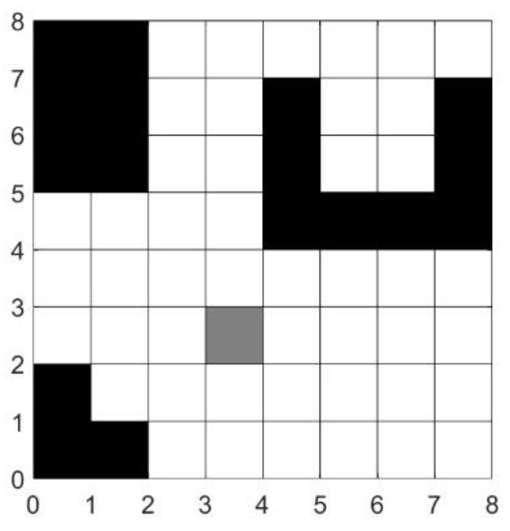
Figure 2.
Child Nodes of the Traditional A* Algorithm.
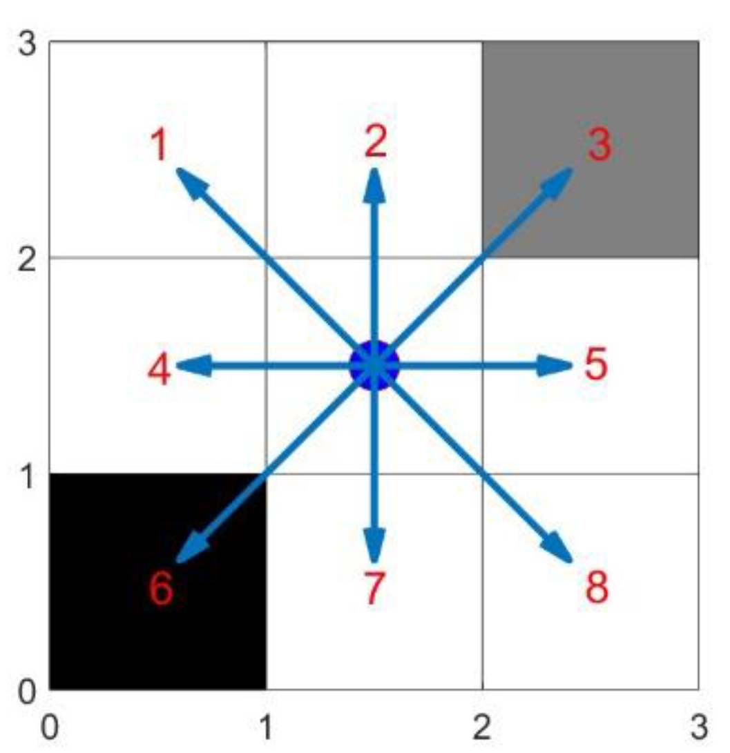
Figure 3.
Pathfinding Flow of the Traditional A* Algorithm.
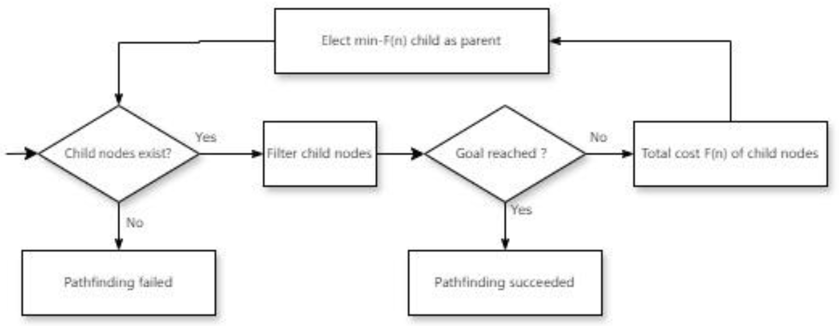
Figure 4.
Example Diagram of Key Point Extraction: (a) Example obstacle; (b) Diagonal positions; (c) Up, down, left, right, and the obstacle itself; (d) Key points.
Figure 4.
Example Diagram of Key Point Extraction: (a) Example obstacle; (b) Diagonal positions; (c) Up, down, left, right, and the obstacle itself; (d) Key points.
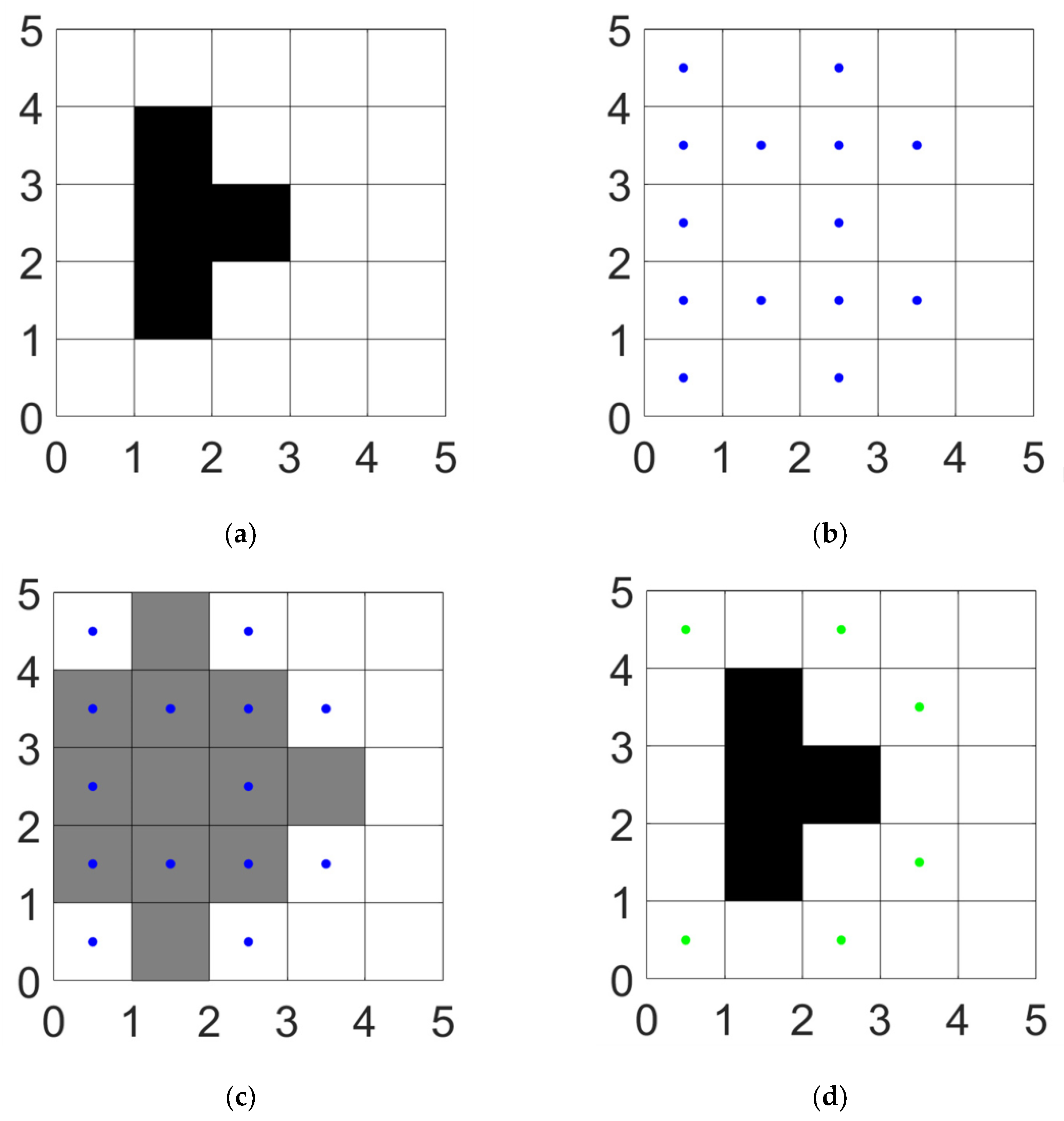
Figure 5.
Extraction of Global Key Points.
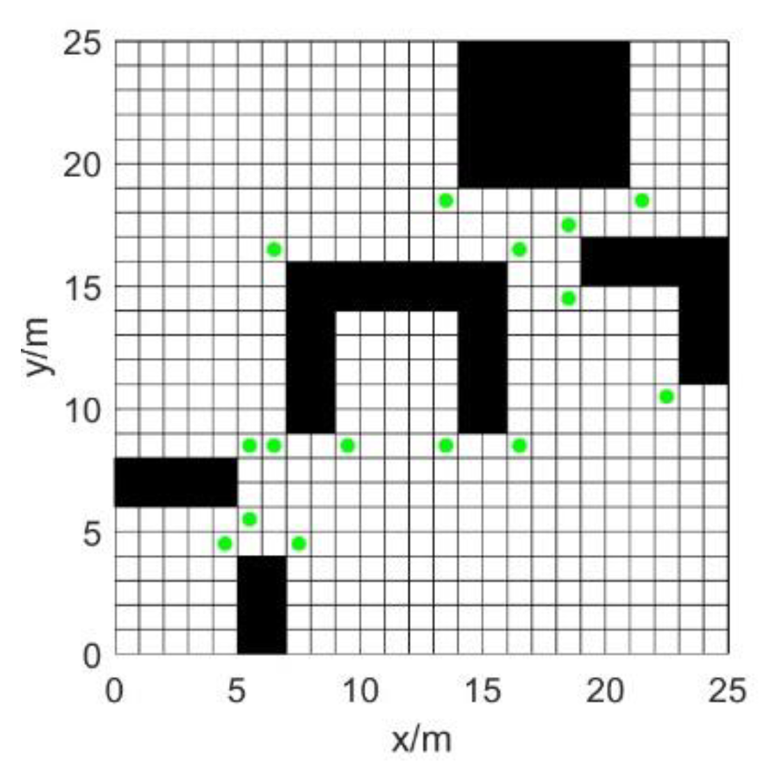
Figure 6.
Child Nodes of the Current Point.
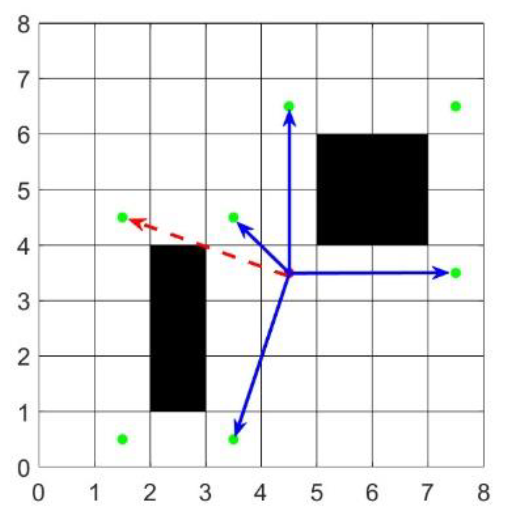
Figure 7.
Decision-Making Flow of the Improved A* Algorithm.
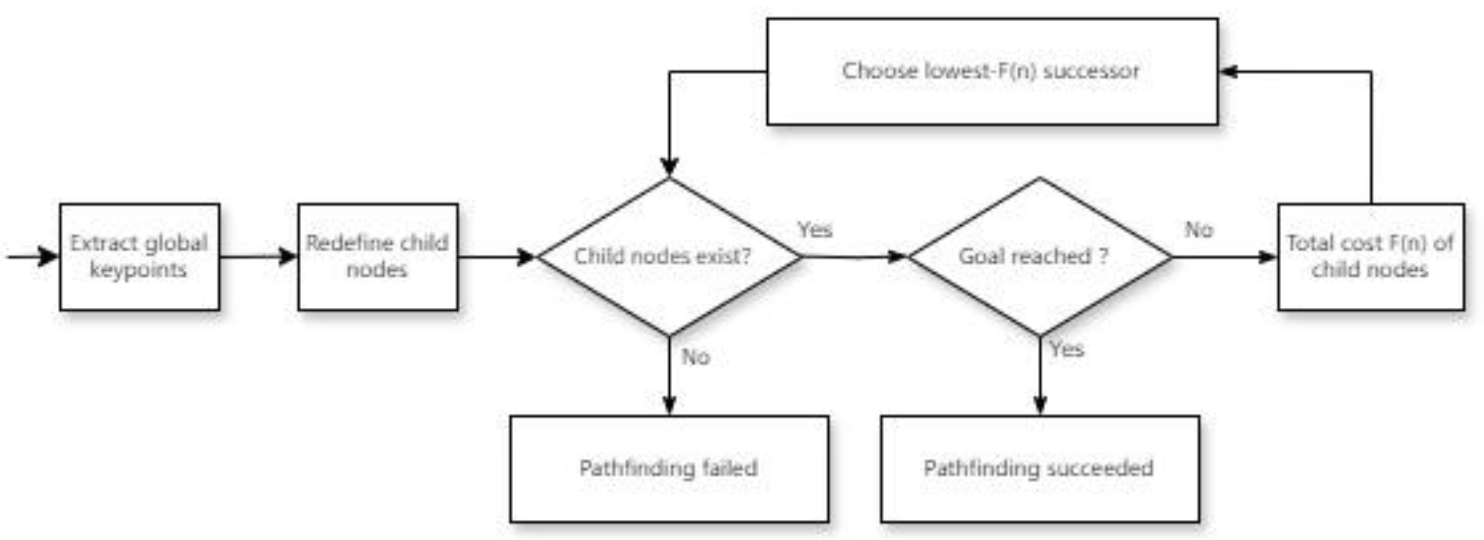
Figure 8.
AGV kinematic model.
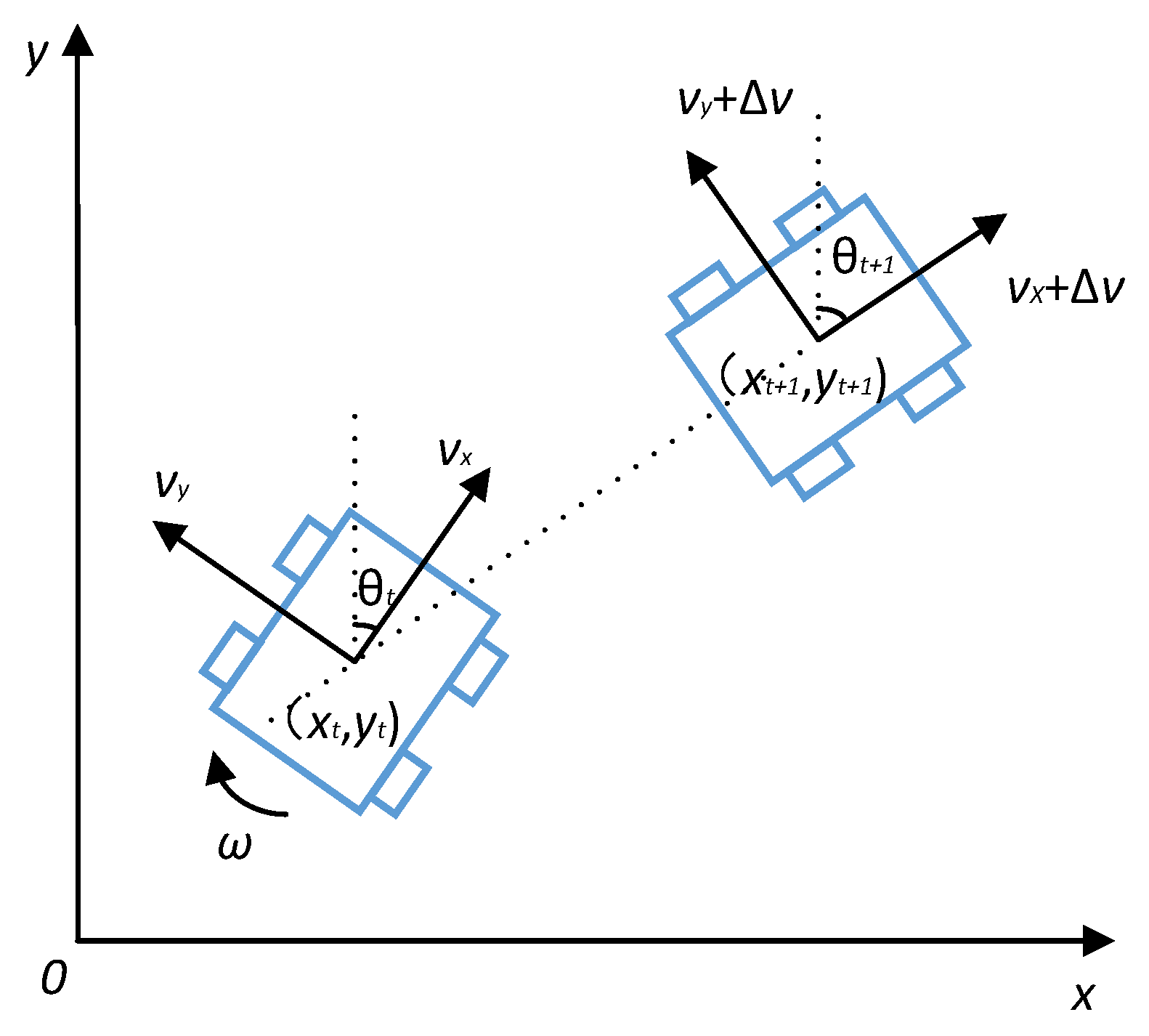
Figure 9.
Flowchart of the hybrid algorithm.
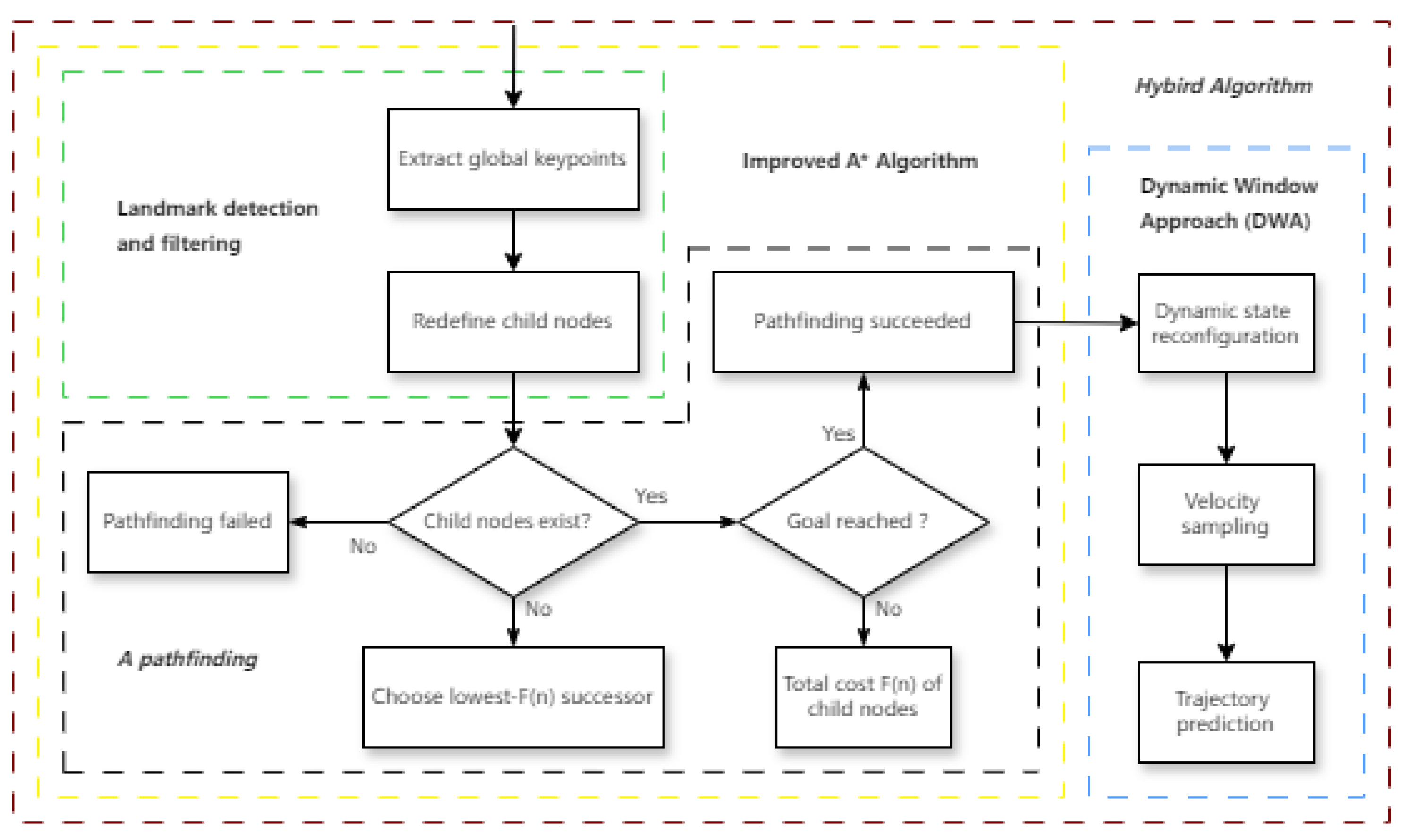
Figure 10.
Comparison of Global Paths Among Several A* Algorithms: (a) Traditional A* Algorithm; (b) Reference[18]; (c) Improved A* Algorithm.
Figure 10.
Comparison of Global Paths Among Several A* Algorithms: (a) Traditional A* Algorithm; (b) Reference[18]; (c) Improved A* Algorithm.
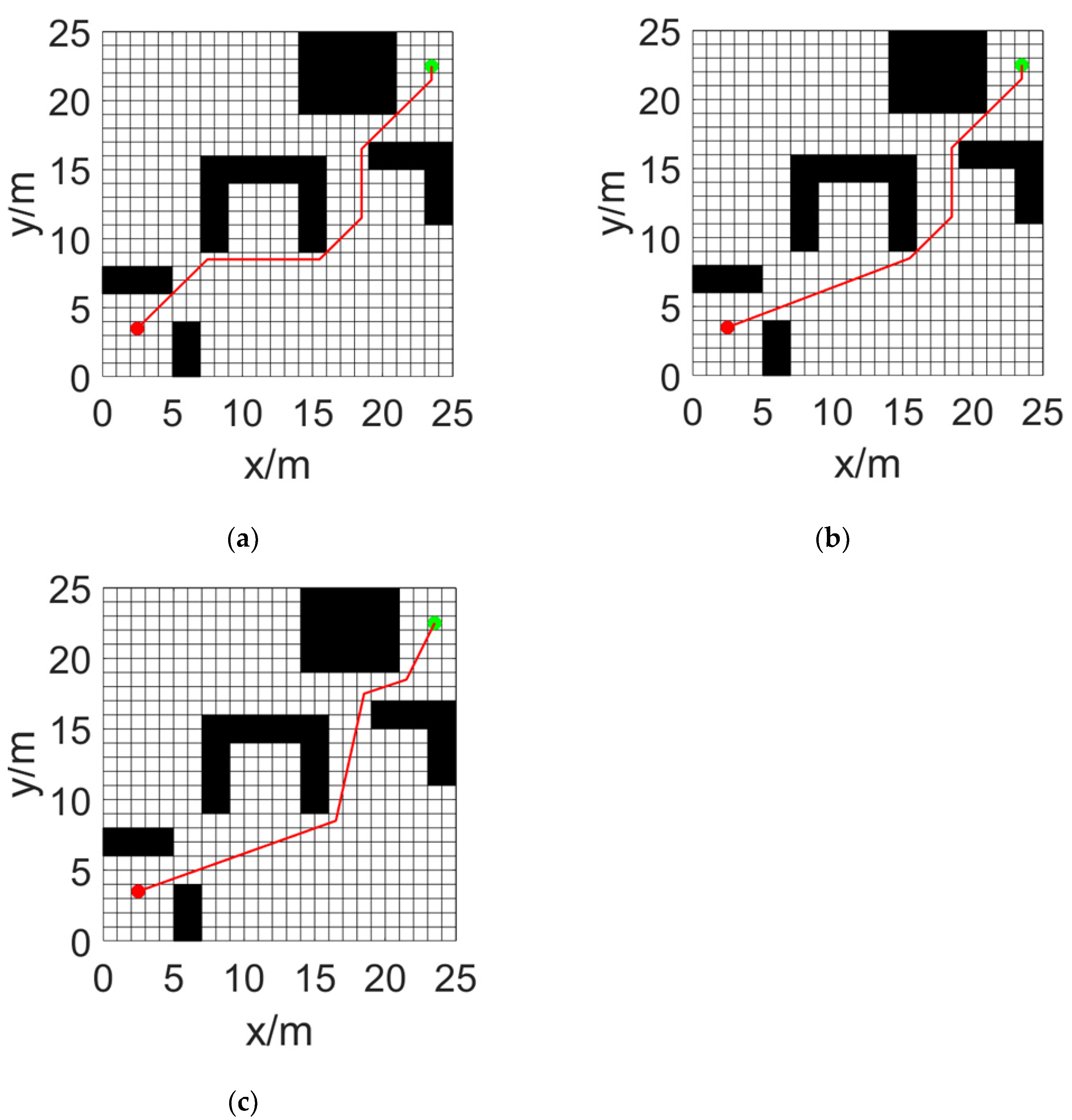
Figure 11.
Path Comparison of the Hybrid Algorithm.
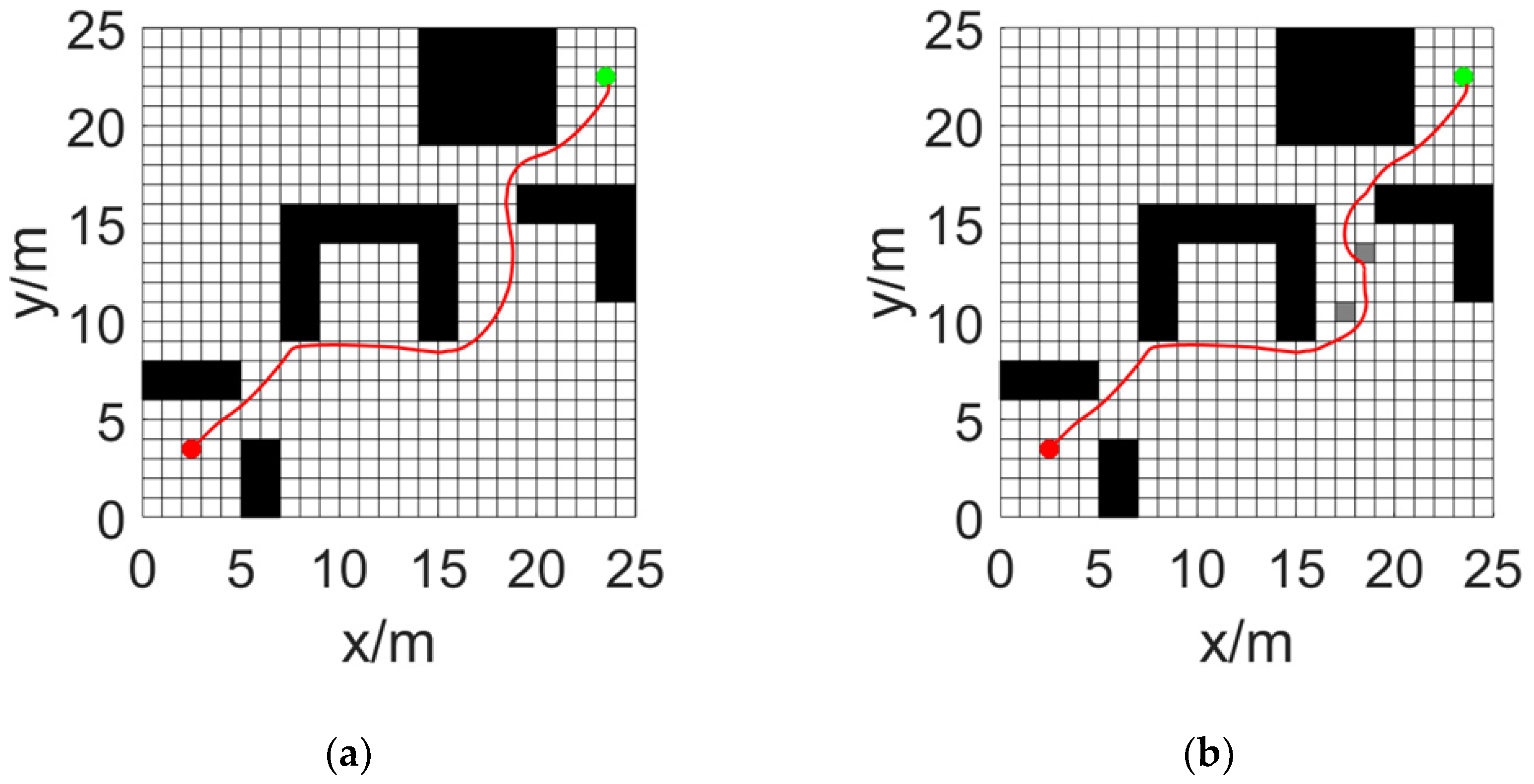
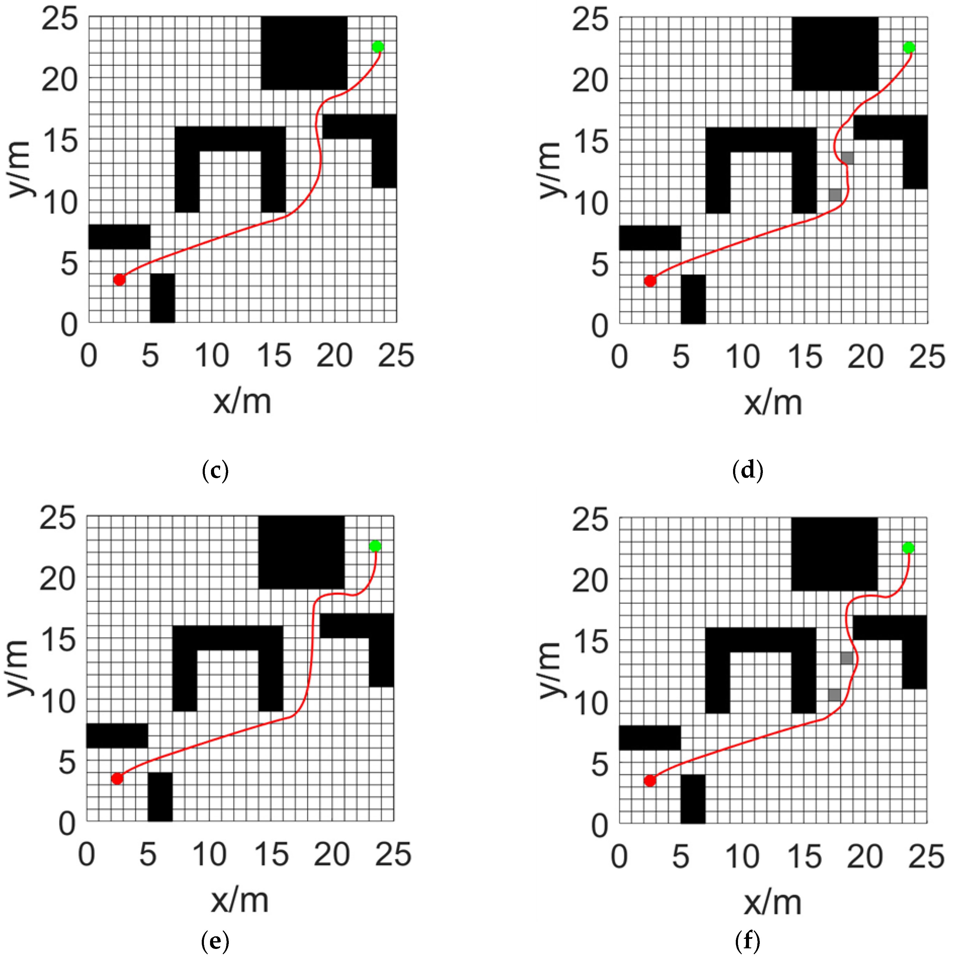
Figure 12.
Variations of Heading Angle, Linear Velocity, and Angular Velocity.
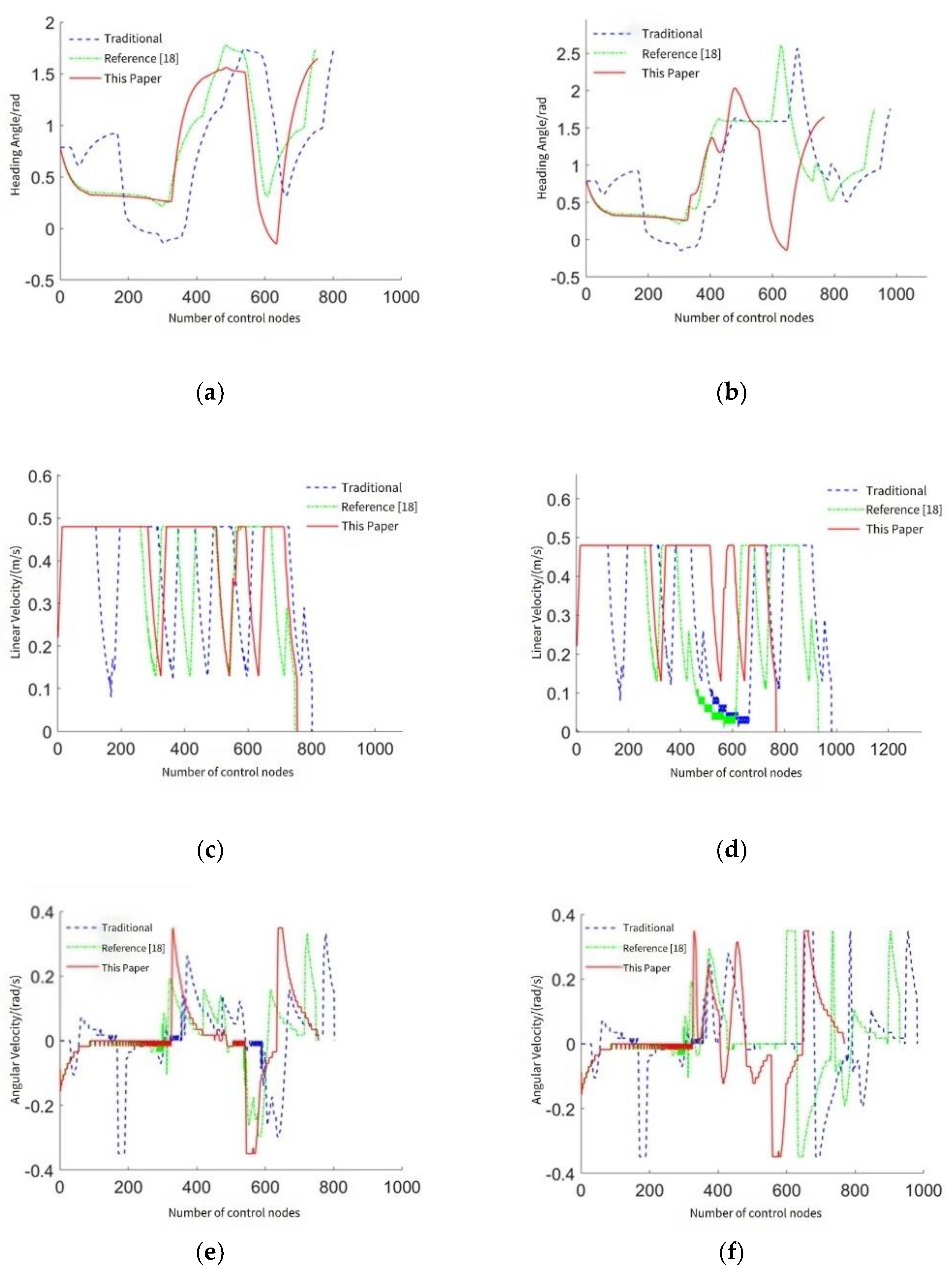
Table 1.
Comparison of Several A* Algorithms.
| Indicator | Traditional A* | Reference [18] | This Paper |
| 0.1827 | 0.1623 | 0.1385 | |
| Inflection Points | 5 | 4 | 3 |
| 32.20 | 31.24 | 31.72 |
1 Tables may have a footer.
Table 2.
AGV Own Attributes.
| Parameter | Value |
| 1.0 | |
| 20.0 | |
| 0.2 | |
| 50.0 | |
| 0.01 | |
| 1.0 |
Table 3.
Initial Attributes of the Dynamic Window Approach (DWA).
| Parameter | Value |
| 0.05 | |
| 0.2 | |
| 0.1 | |
| 3.0 | |
| 0.1 | |
| 0.5 |
Table 5.
Variance of Each Motion Parameter.
| Hybrid Algorithm | Variance | |||
| Variations of Heading Angle | Linear Velocity | Angular Velocity | ||
| Obstacle-Free Env. | Traditional | 0.3147 | 0.0165 | 0.0135 |
| Reference [18] | 0.2463 | 0.0146 | 0.0103 | |
| This Paper | 0.3110 | 0.0119 | 0.0149 | |
| With Random Obstacles | Traditional | 0.3999 | 0.0290 | 0.0176 |
| Reference [18] | 0.3494 | 0.0300 | 0.0156 | |
| This Paper | 0.3502 | 0.0118 | 0.0176 | |
Disclaimer/Publisher’s Note: The statements, opinions and data contained in all publications are solely those of the individual author(s) and contributor(s) and not of MDPI and/or the editor(s). MDPI and/or the editor(s) disclaim responsibility for any injury to people or property resulting from any ideas, methods, instructions or products referred to in the content. |
© 2025 by the authors. Licensee MDPI, Basel, Switzerland. This article is an open access article distributed under the terms and conditions of the Creative Commons Attribution (CC BY) license (http://creativecommons.org/licenses/by/4.0/).
Copyright: This open access article is published under a Creative Commons CC BY 4.0 license, which permit the free download, distribution, and reuse, provided that the author and preprint are cited in any reuse.


