Submitted:
25 October 2025
Posted:
28 October 2025
You are already at the latest version
Abstract
Climate change is expected to have significant yet distinct impacts on arthropods. Studying the species distribution of odonates, which are considered a model taxon for studying climate change and a flagship group for assessing ecosystem health, can reveal potential future patterns of geographic change. My study predicts the impacts of different climate change scenarios on the future habitat and distribution of odonates. I used MaxEnt to construct species distribution models (SDMs) for 30 North American odonate species across seven functional groups, categorized based on functional traits about each genus’s life history, dispersal, morphology, and ecology. Each model was applied to three future years and three different Shared Socio-economic Pathways (SSPs). My results show that odonates will experience increasing overall habitat suitability and increasing range size with shifts northward; however, the total suitable habitat will shrink into smaller, geographically separated pockets. While most functional groups will follow the aforementioned trends, Libellula will experience a decrease in range size, and Aeshna will move the furthest north while experiencing the greatest increase in overall habitat suitability and range size. Overall, SSP5 will result in increased variability among functional groups in their habitat and distribution. This study has implications for understanding invertebrate responses to global change, and may refocus conservation efforts on species with specific functional traits. The functional approach used here may be further applicable to other organisms and regions.
Keywords:
species distribution model
; odonates
; functional group
; habitat
; climate change
; shared socio-economic pathways
1. Introduction
Future anthropogenic climate change [1] will almost inevitably lead to an accelerated loss in biodiversity [2,3]. However, the effects of climate change will vary across species [4,5], making detailed analyses in specific geographic contexts necessary. Meanwhile, the exact magnitude of future climate change will vary significantly based on the choices made for global socio-economic development [2], including greenhouse gas emissions and land use patterns [6]. The Shared Socio-economic Pathways (SSPs), five qualitative narratives describing potential human development trajectories in the 21st century [7,8], outline distinct environmental scenarios [7], providing quantified data to model potential future changes in global biodiversity [7,8,9].
Arthropods are an important component of global biodiversity. Ubiquitously distributed and frequently observed, arthropods provide various important services in ecosystems, such as pollination and decomposition [10]. In future climate change scenarios, arthropods of the same species will experience climate change impacts very differently across distinct habitats [11]. Analyzing future spatial distribution of arthropods is thus relevant for understanding potential changes in their ecosystem services and overall biodiversity.
Among arthropods, odonates, which includes dragonflies and damselflies, has been described as a model taxon [12] for studying the effects of climate change because they are sensitive to both changes in air temperature, which can directly affect water temperature and influence odonate distribution [13], and changes in precipitation patterns, which can affect the structure and organization of odonate microhabitat, such as vernal ponds [14]. Odonates are also often considered a flagship group strongly associated with ecosystem health [15], monitoring and modeling their distributions can potentially reveal wider patterns for freshwater ecosystems even other arthropods. Moreover, as a charismatic taxa [5], abundant historical and current data for odonate distribution is readily available from both scientific research and amateur observation [12].
Odonates possess distinct functional traits that can contribute to wider ecosystem services [12]: as predators, they contribute to pest regulation; as aquatic species sensitive to water quality, they are indicators of freshwater ecosystem health [16]. The diversity of functional traits can contribute to the provision of a wider range of ecosystem services by directly influencing community assembly and function [17,18]. While previous studies have mainly focused on taxonomic classifications [19], this study characterizes species into functional groups based on functional traits. Compared to taxonomic groups, this slightly more flexible approach allows more meaningful interpretations, particularly on how specific communities respond to and influence the environment [3,17].
To understand how odonate functional groups will respond differently to climate change, I built MaxEnt species distribution models to analyze changes to their distributions across future years and SSPs. Species distribution models use algorithms to apply the presence data of a species on selected environmental variables to predict its geographic distribution [20]. Species distribution models have been employed mainly to guide conservation and restoration efforts [20], but could also be helpful when projecting future scenarios under climate change [5]. When an appropriate algorithm is employed [21], this more holistic method could facilitate addressing the complex, nonlinear changes in diversity and distribution [22]. My study thus conducts species distribution modeling on selected functional groups of odonates to predict changes in their habitats in varying future scenarios.
2. Methods
2.1. Defining the Scopes
Following Woods and McGarvey [23], I categorized odonate species into seven functional groups based on 11 functional traits distributed across four categories: life history, dispersal, morphology, and ecology. The seven functional groups were represented by seven specific genera [23] – Argia, Aeshna, Calopteryx, Hetaerina, Libellula, Sympetrum, and Plathemis – based on record abundance. For further details on the functional group classifications, please refer to Woods and McGarvey [23].
I chose the continent of North America, where there are currently only a few existing attempts to apply species distribution models to odonates [5], as the geographic scope. Based on data accessibility, my study roughly considered North America as all land within the range of 180∘W to 50∘W and 5∘N to 85∘N. This definition included all land masses and islands around the North American continent, except for parts of Greenland.
My study modeled odonate distributions in 2020, 2050, 2075, and 2100. The year 2020 served as a baseline for the construction of the models before they were applied to future scenarios due to the availability of data on environmental variables. The subsequent 25-year intervals were a balance between the aim of modeling gradual changes in detail and the reality of computational limitations.
The Shared Socio-economic Pathways (SSPs) provide narratives that help define the scope of future variability. To capture a wider range of estimates for future odonate distributions while balancing computational demands and limited availability of future predictive data, I selected three SSPs: SSP1-2.6, in which the world gradually shifts to sustainable development, achieving relatively low levels of climate change; SSP2-4.5, in which the world follows a steady, typical development pathway; and SSP5-8.5, in which development is accelerated by increased use of fossil fuel, leading to more drastic effects of climate change.
2.2. Retrieving and Cleaning Data
Presence-only data for North American odonates was retrieved from the Odonata Central dataset [24] hosted on the Global Biodiversity Information Facility (GBIF) platform. The download on April 26, 2025 with 248,533 records [25] was filtered to include only North American records during the period 2015–2025 to align with the defined geographic and temporal scopes, so that historical or geographically irrelevant records do not interfere with the analysis. The data were cleaned using the package pandas (Python, version 2.2.3) [26]. Since our study would explicitly focus on the seven representative genera in North America, all records irrelevant to the selected genera were removed. Since the performance of species distribution models tend to decrease at low species occurrences [21], among all 129 species across the seven selected genera, 41 of them with less than 30 occurrence records were removed. A maximum of 5 species with the most occurrence records were selected from the remaining species in each of the seven genera; notably, there were only 2 existing species in the genus Plathemis, and only 3 Hetaerina species had enough records to be included in the analysis. After unnecessary entries were removed, the remaining 59,307 records, covering a total of 30 species under the seven genera as described in Table 1, were used as presence points in the model.
To capture a range of variables that may influence odonate species distribution, I included climate, human population density, and land use changes in my analysis. Climate has been the primary determinant of species distribution at a continental spatial scale [27]. I retrieved future predictions of 19 bioclimatic variables based on the output of the HadGEM3-GC31-LL global climate model from WorldClim [28]. These predictions, with a spatial resolution of 2.5 , were presented as averages over 20-year periods ranging from 2021–2040 to 2081–2100 under three SSP scenarios. I cropped the dataset to the defined geographic scope and rescaled it to a resolution of 1 using the package terra (R, version 1.8-5) [29].
Human population density could also help account for future anthropogenic influences on the habitats of odonates [5]. Future predictions of population density at 5-year intervals with a spatial resolution of 1 were retrieved from [30], then cleaned to the defined geographic scope using the package terra (R, version 1.8-5) [29].
Land use changes, which have rarely been included in existing species distribution models [5], may similarly influence the habitats of odonates. Future predictions of land use at 5-year intervals with a spatial resolution of 1 were retrieved from [31], transposed to ensure that the x and y axes match longitude and latitude, respectively, using the package xarray (Python, version 2025.1.1) [32], then cleaned to the defined geographic scope using the package terra (R, version 1.8-5) [29]. All land uses for irrigated crops were combined in a single new “Irrigated Crops Cumulative” category, and rainfed crops in “Rainfed Crops Cumulative”.
Selected topographic factors, such as slope, could also influence drainage basin characteristics and thus the distribution of odonates [5]. Unlike other factors, topographic data would likely have few changes throughout the defined temporal scope and were therefore modeled consistently across all the selected years. Slope and terrain roughness data with a spatial resolution of 1 was retrieved from [33], then cleaned to the defined geographic scope using the package terra (R, version 1.8-5) [29].
2.3. Selecting Background Points and Environmental Variables
Since the Odonata Central database provided presence-only data, which contains information on observed species presence but not absence [34], pseudo-absence background points were randomly sampled to facilitate the construction of species distribution models [21]. Increasing the number of background points could capture a more comprehensive sample of most potential combinations of environmental factors, allowing for a better performance, but would simultaneously bring a higher computational burden [21]. Nine preliminary MaxEnt models were fitted to different numbers of background points (256 to 65,536). All retrieved variables were included without further selection. The species Aeshna sedula was selected for the preliminary model since it had 1,866 records in total, close to the mean number of records, 1,976.9, of all 30 selected species. To balance performance and runtime, 8,192 background points were used in all subsequent models.
Multicollinearity between the bioclimatic, land use, human population density, and topographic variables was assessed with variable inflation factor (VIF) test using the package usdm (R, version 2.1-7) [35]. I adopted a relatively lenient VIF threshold of 25, reflecting the large sample size and the high variance of the independent variable [36]. After 18 variables were removed, the multicollinearity of the remaining 22 environmental variables (Table 2) satisfied the selected threshold.
I conducted a second round of screening to select the main environmental variables [37,38]. For each of the 30 species (Table 1), an initial MaxEnt species distribution model with presence records and background points was fitted to all 22 remaining variables using the maxent function in the package dismo (R, version 1.3-16) [39]. All variables that did not meet a permutation importance threshold of 2.5 were dropped for the respective species; the remaining variables were included in the final models. The number of selected variables ranged from 3 for Sympetrum ambiguum to 10 for Argia fumipennis, Hetaerina vulnerata, Plathemis lydia, and Sympetrum corruptum.
2.4. Constructing Final Species Distribution Models
MaxEnt (maximum entropy) [40] is considered an efficient and well-performing option for species distribution models [21]. MaxEnt is a machine-learning technique that estimates probability distributions from incomplete information that are closest to uniform, calculated under the constraint that the expected value of each environmental variable under this estimated distribution matches the empirical average from the species occurrence data [40]. It was also specifically designed for handling presence-only data [40], suitable for the Odonata Central database [24].
The 8,192 background points were randomly sampled from the defined geographic scope, then combined with the existing presence-only data for each of the 30 species. The combined data was randomly divided through an 80:20 train-test split using the folds function in the package predicts (R, version 0.1-17) [41]. The larger training set was used to construct a final MaxEnt model based on the environmental variables selected through the initial models for the baseline year of 2020 using the maxent function in the R package dismo (R, version 1.3-16) [39]. The smaller testing set was used to evaluate the final model through the area under the receiver operating characteristic curve (), a number within the range , using the pa_evaluate function in the package predicts (R, version 0.1-17) [41]. A random prediction would result in , while would indicate that the model was well-fitted [42]. The 30 models for the species had a mean testing with a standard deviation of , suggesting that all models were well-fitted.
The models were then extrapolated to each of the year-SSP combinations in the defined temporal and variability scopes. The output for each estimation was given in the form of a continuous estimate of suitability from 0 to 1; a higher value indicates greater suitability. The average estimate of suitability throughout the defined geographic scope was recorded as the overall habitat suitability.
A threshold was used to convert the model’s continuous estimate into a binary prediction. The maximum sum of specificity sensitivity (maxSSS) threshold would find the highest value of the sum of specificity (true presences) and sensitivity (true absences) [43]. This threshold has been proven effective in previous studies [44,45] and was especially suitable for this scenario due to the abundance of presence data points [44]; though traditionally used on presence-absence data, it has demonstrated good performance on presence-only data [43]. In the resulting binary prediction, range size was defined as the area of all 1 grids predicted as the habitat. The centroid, a coordinate pair, was calculated as the mean coordinate of all grids marked as the predicted habitat. Range size and centroid were recorded for each species under each year-SSP combination.
In total, each model returned three key outputs for analysis. Overall habitat suitability was the mean of the direct predictive output of the species distribution model – a value between 0 and 1 – under the defined geographic scope. Range size was the total area of a species’ predicted habitat obtained by applying the maximum sensitivity specificity sum (maxSSS) threshold to the direct output of the species distribution model. Centroid change was the Euclidean distance between the geometric centroid of the predicted habitat of a species in a specific future scenario and the geometric centroid of the habitat in the baseline year of 2020.
2.5. Analysis
Changes between each of the predicted future scenarios and the baseline scenario of the respective species were calculated based on the raw outputs of the MaxEnt models. Percent change from baseline was calculated for overall habitat suitability and range size, while Euclidean distance from baseline was calculated for centroid.
A linear model was fit to the log-transformed response variables using lm function from stats (R, version 4.4.3) [46], with year as an independent variable alongside SSP and genus as interacting terms. Logarithmic transformation was applied to account for the non-negative, right-skewed nature of the data. Since the models on overall habitat suitability and range size did not meet all assumptions of residual normality, we performed non-parametric bootstrapping using the package boots (R, version 1.3-31) [47] to evaluate the stability of coefficient estimates and confidence intervals. Most of the resulting confidence intervals of the coefficients were within acceptable ranges to validate the linear models, though slight deviations for the interacting factors of SSP2:Hetaerina and SSP2:Plathemis, presumably due to the lower number of selected species in the respective genera, suggests that these particular results should be interpreted with more caution.
Marginal means for each genus and each SSP scenario were then calculated using the R package emmeans [48], allowing direct comparison across genera and SSPs. Statistical significance was evaluated through a non-parametric assessment on the 95% confidence intervals of the marginal means [49]. Furthermore, the permutation importance of each environmental variable, calculated as the normalized percent decrease in training AUC after random permutation of its values [50], was retrieved from the final models to assess which environmental variables were more significant at influencing odonate habitats; variables excluded from the initial models, and thus unused in the final models, were considered to have a permutation importance of 0.
3. Results
3.1. Overall Habitat Suitability Changes
All seven functional groups showed an increase in overall habitat suitability, which reflects whether the environment across North America is generally more or less conducive to the survival of a species (Figure 1), with six groups being statistically significant. Aeshna (, ) will experience the largest increase. Sympetrum (, ), Hetaerina (, ), and Calopteryx (, ) shared similar and overlapping predictions. The exception is the functional group represented by Libellula (, ), whose increase in overall habitat suitability is not statistically significant, suggesting a potential future risk of competitive disadvantage, vulnerability, and the need for conservation focus compared to the other species.
The effects of SSP scenarios varied across genera (Figure 2). SSP1, which describes more sustainable development, displayed the smallest differences between functional groups, consistently leading to slight increases ranging from (Sympetrum) to (Aeshna). By contrast, SSP5, which describes an accelerated climate change, led to the largest differences between predicted changes and current suitability, resulting in a considerable increase in overall habitat suitability for functional groups such as those represented by Aeshna () and Hetaerina (). In some functional groups, however, the effects of SSP was not significant, such as those represented by Calopteryx (SSP1 , SSP5 ) and Libellula (SSP1 , SSP5 ).
3.2. Range Size Changes
Range size change across functional groups, which reflects whether more or less area is considered favorable for the genera, similarly increased (Figure 3). All functional groups but Libellula (, ) were predicted to have a greater range size, from Sympetrum (, ) to Aeshna (, ). For three of the seven functional groups (Libellula, Sympetrum, and Calopteryx), the predicted increase in range size was not statistically significant.
Varying effects of SSP on range size across functional groups also resembled the results on overall habitat suitability (Figure 4). SSP1 generally displayed the smallest differences between functional groups, leading to slight changes ranging from (Sympetrum) to (Aeshna). SSP5 led to the largest differences between functional groups, with Aeshna increasing (), and Libellula decreasing ().
3.3. Centroid Change
Centroid change, or how far a species has migrated from its original habitat, varied significantly among species (Figure 5). The functional group represented by Aeshna was predicted to experience the greatest centroid change (, ), with a statistically significant difference compared to all the other functional groups, followed by a more moderate change experienced by the functional group represented by Sympetrum (, ). The functional groups represented by Libellula, Plathemis, and Argia were the least affected with a centroid change of ; they also had the narrowest confidence intervals, suggesting prediction robustness.
The effects of SSP on centroid were consistent across functional groups (Figure 6). SSP5 led to the highest change in centroid, with a change of for Aeshna. SSP2, the intermediate scenario, typically led to a moderate change, ranging from 48.069% (Libellula) to 71.075% (Hetaerina) compared to the changes shown in SSP5 scenarios. SSP1 resulted in the lowest changes overall, such as merely for Plathemis, again suggesting how this more sustainable scenario could bring more certainty and assurance to future conservation efforts.

Table 3.
Summary of marginal means and confidence intervals, grouped by genus, for overall habitat suitability (adjusted by ), range size (adjusted by ), and range centroid distance change.
Table 3.
Summary of marginal means and confidence intervals, grouped by genus, for overall habitat suitability (adjusted by ), range size (adjusted by ), and range centroid distance change.
| Genus | General Suitability (%) | Range Size (%) | Centroid Distance () | |||
| Aeshna | ||||||
| Argia | ||||||
| Calopteryx | ||||||
| Hetaerina | ||||||
| Libellula | ||||||
| Plathemis | ||||||
| Sympetrum | ||||||
3.4. Environmental Variable Permutation Importance
Permutation importance of environmental variables were collected from the final models to evaluate their influence on odonate distributions (Figure 7). The results suggested that bioclimatic variables, especially temperature-related variables like Annual Mean Temperature (BIO1, , ) were a particularly strong determinant of odonate distributions, followed by Annual Mean Precipitation (BIO12, , ) and Temperature Annual Range (BIO7, , ). Selected land use types like Needleleaf Evergreen Tree Boreal (PFT2, , ) and Human Population Density (HPD, , ) also had relatively significant contributions. However, most land use types, as well as topographic slope (, ), had much smaller influence overall, suggesting that they had low relevance to odonate species distribution.
4. Discussion
The results of MaxEnt and linear models revealed that the aggregate habitat of all odonate functional groups will shift to the north and expand into smaller pockets, with the greatest changes observed under SSP5. Among the environmental predictor variables, bioclimatic variables such as Annual Mean Temperature (BIO1) showed the most significant impact. Significant differences were observed between functional groups, indicating a functional approach to species distribution modeling under global change scenarios may be an effective way to understand potential changes to ecosystem services.
The statistically significant predictions on distance shift indicate that all odonate species will migrate to the north (polewards) in the coming decades. This kind of habitat shift may be feasible for odonates since North America does not have major east-west geographic constraints, such as the Alps in Europe, that would prevent such movement [12]. However, the habitat shift of odonates may trigger chain reactions leading to habitat shifts of multiple related species in a shared ecosystem [51], creating new challenges and opportunities for species conservation of and beyond odonates.
Notably, stronger habitat changes compared to the baseline scenario and greater differences between functional groups are observed under SSP5, the trajectory with more severe global warming. All species are expected to shift further to the north. Species whose overall suitabilities are predicted to increase will have even larger range sizes, while species with lower overall suitabilities will likely require more conservation attention. This highlights the uncertainty that a less sustainable pathway might bring to future biodiversity and conservation efforts, underscoring the necessity to reduce carbon emissions to meet the 2 degrees climate target [52].
As the habitat of species shifts to the north in future decades, many will encounter changes in landforms that split a species into relatively isolated smaller fragments, potentially leading to a loss in genetic diversity within a species and eventually higher extinction risks [53]. This is supported by the model’s predictions that range size is predicted to increase slower than overall habitat suitability. As a case study, the predicted distribution changes for Calopteryx angustipennis, or Appalachian Jewelwing, in 2100 under SSP5 shows a drastic shift to the north from its baseline distribution in southern United States to enter Canada (Figure 8). Compared to the current large cluster in the southeastern United States, the species will likely split into four smaller fragments, occupying Nova Scotia, the tri-state area, the Great Lakes, and the peaks of the Appalachian Mountains.
Of all the environmental variables used to predict future habitat changes, the high permutation importance of all temperature variables lends further support to the projected impacts of climate on odonates [5,12]. On the other hand, slope and many land use types had low permutation importance. Future efforts at modeling species distribution should focus more on climatic variables, but can potentially keep the few most relevant land use types for odonates in the region, such as Needleleaf Evergreen Tree Boreal (PFT2) in North America, as supplementary determinants.
The models and analyses have some limitations worth further consideration. Geographically, the isolation between the eastern and western sides of North America can lead to overprediction of species distributions. Since major north-south features in North America, such as the Rocky Mountains and the Great Plains, can prevent east-to-west migration, a species from one side of North America would be unable to colonize a region on the other side even if the climate and land use patterns are similar. For instance, though C. angustipennis is currently only found in the southeastern states [24], the baseline model falsely suggested an additional tiny piece of C. angustipennis habitat in central Mexico, where similar environmental variables are present (Figure 8). The model could thus potentially overpredict overall habitat suitability and range size and shift all range centroids to the west. However, this consideration applies to all predictions, including the baseline year and in future scenarios. Since the final analyses compare the future changes to the baseline year, the generalizable results still reflect relatively accurate changes throughout the years. Additionally, the uneven representation across genera, from 2 for Plathemis to 5 for the other genera, resulted in stronger uncertainties in functional groups represented by less species, limiting the strength of interpretation.
Despite potential limitations, this study’s results can help to design conservation strategies. Of the seven representative genera included in the study, species with negative predicted range size changes and higher habitat fragmentation should be considered more vulnerable and ought to be prioritized in conservation efforts. Such conservation efforts can be applied to other genera in the same functional group. Alternatively, the more vulnerable functional groups identified by my study can be primary targets for additional species distribution modeling to further specify the variations within the functional groups.
Though the study was limited to North America, it would be important to project the methods and findings of the study to a global scope. Species distribution modeling has only been applied to less than a quarter of all discovered odonate species [5]. Since the current study revealed that responses to climate change could vary significantly among functional groups, more modeling attempts would be necessary to discover patterns for different functional groups in other spatial contexts. Notably, the quality of presence data in other spatial contexts can be vulnerable to sample selection bias, in which more presence observations are recorded in easily accessible areas [55], which can be mitigated by extracting such bias from the presence-only dataset to be intentionally introduced when selecting background points [55]. Meanwhile, the study can also include other potential environmental variables for more robust predictions. For instance, data describing river characteristics such as water chemistry [5] and agrochemical usage [56] could impact earlier stages of odonate life cycle, especially naiads, and thus influence the distribution of adult odonates [5]: potential anthropogenic damages to water quality, for example, might reduce future habitats for odonates. Beyond modeling with environmental variables, some studies have highlighted the interactive effects of flora and vegetation on odonate abundance [57]; however, others have found weaker correlations between plant diversity and odonate distribution, instead recommending the current approach[58]. Expanding the scope of the study could help identify the causes of nonlinear variations in predicted biodiversity changes, facilitating the conservation of important practical and cultural values in diverse ecosystems [3].
By modeling the distribution of North American odonate functional groups using MaxEnt, this study took a novel approach to categorizing species for species distribution modeling and provided insights into the future distribution of odonates under climate change scenarios. In particular, most functional groups will experience northward range expansions, increased habitat suitability, and greater fragmentation, with effects amplified under SSP5 and Libellula experiencing potential range contractions. These findings emphasize the need for targeted conservation strategies tailored to each functional group under different climate scenarios, especially in functional groups predicted to suffer from habitat fragmentation. Future research can consider adapting the functional-group-based approach to other taxonomic groups and geographic regions to provide critical insights for conservation planning that considers both species vulnerability and cascading effects on ecosystem services.
Funding
This research received no external funding.
Data Availability Statement
No new data were created in this study. The original analysis presented in the study is available from https://doi.org/10.5281/zenodo.17427083.
Acknowledgments
I would like to thank Dr. Nathalie Sommer for her invaluable guidance throughout this research.
Conflicts of Interest
The author declares no conflicts of interest.
References
- IPCC. Climate Change 2001: The Scientific Basis; 2001.
- Pereira, H.M.; Leadley, P.W.; Proença, V.; Alkemade, R.; Scharlemann, J.P.W.; Fernandez-Manjarrés, J.F.; Araújo, M.B.; Balvanera, P.; Biggs, R.; Cheung, W.W.L.; et al. Scenarios for Global Biodiversity in the 21st Century. Science 2010, 330, 1496–1501. [Google Scholar] [CrossRef]
- Chapin III, F.S.; Zavaleta, E.S.; Eviner, V.T.; Naylor, R.L.; Vitousek, P.M.; Reynolds, H.L.; Hooper, D.U.; Lavorel, S.; Sala, O.E.; Hobbie, S.E.; et al. Consequences of changing biodiversity. Nature 2000, 405, 234–242. [Google Scholar] [CrossRef]
- Bellard, C.; Bertelsmeier, C.; Leadley, P.; Thuiller, W.; Courchamp, F. Impacts of climate change on the future of biodiversity. Ecology Letters 2012, 15, 365–377. [Google Scholar] [CrossRef]
- Collins, S.D.; McIntyre, N.E. Modeling the distribution of odonates: a review. Freshwater Science 2015, 34, 1144–1158. [Google Scholar] [CrossRef]
- Riahi, K.; Van Vuuren, D.P.; Kriegler, E.; Edmonds, J.; O’Neill, B.C.; Fujimori, S.; Bauer, N.; Calvin, K.; Dellink, R.; Fricko, O.; et al. The Shared Socioeconomic Pathways and their energy, land use, and greenhouse gas emissions implications: An overview. Global Environmental Change 2017, 42, 153–168. [Google Scholar] [CrossRef]
- O’Neill, B.C.; Kriegler, E.; Ebi, K.L.; Kemp-Benedict, E.; Riahi, K.; Rothman, D.S.; Van Ruijven, B.J.; Van Vuuren, D.P.; Birkmann, J.; Kok, K.; et al. The roads ahead: Narratives for shared socioeconomic pathways describing world futures in the 21st century. Global Environmental Change 2017, 42, 169–180. [Google Scholar] [CrossRef]
- Van Vuuren, D.P.; Riahi, K.; Calvin, K.; Dellink, R.; Emmerling, J.; Fujimori, S.; Kc, S.; Kriegler, E.; O’Neill, B. The Shared Socio-economic Pathways: Trajectories for human development and global environmental change. Global Environmental Change 2017, 42, 148–152. [Google Scholar] [CrossRef]
- Kok, M.T.J.; Kok, K.; Peterson, G.D.; Hill, R.; Agard, J.; Carpenter, S.R. Biodiversity and ecosystem services require IPBES to take novel approach to scenarios. Sustainability Science 2017, 12, 177–181. [Google Scholar] [CrossRef]
- Price, P.W.; Denno, R.F.; Eubanks, M.D.; Finke, D.L.; Kaplan, I. Insect Ecology: Behavior, Populations and Communities, 1 ed.; Cambridge University Press, 2011. [Google Scholar] [CrossRef]
- Thomas, J.A.; Rose, R.J.; Clarke, R.T.; Thomas, C.D.; Webb, N.R. Intraspecific variation in habitat availability among ectothermic animals near their climatic limits and their centres of range. Functional Ecology 1999, 13, 55–64. [Google Scholar] [CrossRef]
- Hassall, C.; Thompson, D.J. The effects of environmental warming on Odonata: a review. International Journal of Odonatology 2008, 11, 131–153. [Google Scholar] [CrossRef]
- Caissie, D. The thermal regime of rivers: a review. Freshwater Biology 2006, 51, 1389–1406. [Google Scholar] [CrossRef]
- Buisson, L.; Thuiller, W.; Lek, S.; Lim, P.; Grenouillet, G. Climate change hastens the turnover of stream fish assemblages. Global Change Biology 2008, 14, 2232–2248. [Google Scholar] [CrossRef]
- Oertli, B.; Joye, D.A.; Castella, E.; Juge, R.; Cambin, D.; Lachavanne, J.B. Does size matter? The relationship between pond area and biodiversity. Biological Conservation 2002, 104, 59–70. [Google Scholar] [CrossRef]
- May, M.L. Odonata: Who They Are and What They Have Done for Us Lately: Classification and Ecosystem Services of Dragonflies. Insects 2019, 10. [Google Scholar] [CrossRef]
- Nock, C.A.; Vogt, R.J.; Beisner, B.E. Functional Traits. In Encyclopedia of Life Sciences, 1 ed.; Wiley, 2016; pp. 1–8. [Google Scholar] [CrossRef]
- Cadotte, M.W.; Carscadden, K.; Mirotchnick, N. Beyond species: functional diversity and the maintenance of ecological processes and services. Journal of Applied Ecology 2011, 48, 1079–1087. [Google Scholar] [CrossRef]
- Renault, D.; Leclerc, C.; Colleu, M.; Boutet, A.; Hotte, H.; Colinet, H.; Chown, S.L.; Convey, P. The rising threat of climate change for arthropods from Earth’s cold regions: Taxonomic rather than native status drives species sensitivity. Global Change Biology 2022, 28, 5914–5927. [Google Scholar] [CrossRef]
- Rathore, M.K.; Sharma, L.K. Efficacy of species distribution models (SDMs) for ecological realms to ascertain biological conservation and practices. Biodiversity and Conservation 2023, 32, 3053–3087. [Google Scholar] [CrossRef]
- Valavi, R.; Guillera-Arroita, G.; Lahoz-Monfort, J.J.; Elith, J. Predictive performance of presence-only species distribution models: a benchmark study with reproducible code. Ecological Monographs 2022, 92, e01486. [Google Scholar] [CrossRef]
- Høye, T.T.; Loboda, S.; Koltz, A.M.; Gillespie, M.A.K.; Bowden, J.J.; Schmidt, N.M. Nonlinear trends in abundance and diversity and complex responses to climate change in Arctic arthropods. Proceedings of the National Academy of Sciences 2021, 118, e2002557117. [Google Scholar] [CrossRef] [PubMed]
- Woods, T.; McGarvey, D.J. Drivers of Odonata flight timing revealed by natural history collection data. Journal of Animal Ecology 2023, 92, 310–323. [Google Scholar] [CrossRef] [PubMed]
- Abbott, J.C. Odonata Central, 2025. [CrossRef]
- GBIF.org. Occurrence Download, 2025. [CrossRef]
- The Pandas Development Team. pandas-dev/pandas: Pandas, 2020. [CrossRef]
- Pearson, R.G.; Dawson, T.P. Predicting the impacts of climate change on the distribution of species: are bioclimate envelope models useful? Global Ecology and Biogeography 2003, 12, 361–371. [Google Scholar] [CrossRef]
- Fick, S.E.; Hijmans, R.J. WorldClim 2: new 1-km spatial resolution climate surfaces for global land areas. International Journal of Climatology 2017, 37, 4302–4315. [Google Scholar] [CrossRef]
- Hijmans, R.J. terra: Spatial Data Analysis; 2024.
- Wang, X.; Meng, X.; Long, Y. Projecting 1 km-grid population distributions from 2020 to 2100 globally under shared socioeconomic pathways. Scientific Data 2022, 9, 563. [Google Scholar] [CrossRef]
- Chen, M.; Vernon, C.R.; Graham, N.T.; Hejazi, M.; Huang, M.; Cheng, Y.; Calvin, K. Global land use for 2015–2100 at 0.05° resolution under diverse socioeconomic and climate scenarios. Scientific Data 2020, 7, 320. [Google Scholar] [CrossRef]
- Hoyer, S.; Joseph, H. xarray: N-D labeled Arrays and Datasets in Python. Journal of Open Research Software 2017, 5. [Google Scholar] [CrossRef]
- Amatulli, G.; Domisch, S.; Tuanmu, M.N.; Parmentier, B.; Ranipeta, A.; Malczyk, J.; Jetz, W. A suite of global, cross-scale topographic variables for environmental and biodiversity modeling. Scientific Data 2018, 5. Publisher: Springer Science and Business Media LLC. [Google Scholar] [CrossRef] [PubMed]
- Pearce, J.L.; Boyce, M.S. Modelling distribution and abundance with presence-only data. Journal of Applied Ecology 2006, 43, 405–412. [Google Scholar] [CrossRef]
- Naimi, B.; Hamm, N.a.s.; Groen, T.A.; Skidmore, A.K.; Toxopeus, A.G. Where is positional uncertainty a problem for species distribution modelling. Ecography 2014, 37, 191–203. [Google Scholar] [CrossRef]
- O’Brien, R.M. A Caution Regarding Rules of Thumb for Variance Inflation Factors. Quality & Quantity 2007, 41, 673–690. [Google Scholar] [CrossRef]
- Schnase, J.L.; Carroll, M.L. Automatic variable selection in ecological niche modeling: A case study using Cassin’s Sparrow (Peucaea cassinii). PLOS ONE 2022, 17, e0257502. [Google Scholar] [CrossRef] [PubMed]
- Ab Lah, N.Z.; Yusop, Z.; Hashim, M.; Mohd Salim, J.; Numata, S. Predicting the Habitat Suitability of Melaleuca cajuputi Based on the MaxEnt Species Distribution Model. Forests 2021, 12, 1449. [Google Scholar] [CrossRef]
- Hijmans, R.J.; Phillips, S.; Leathwick, J.; Elith, J. dismo: Species Distribution Modeling; 2024.
- Phillips, S.J.; Anderson, R.P.; Schapire, R.E. Maximum entropy modeling of species geographic distributions. Ecological Modelling 2006, 190, 231–259. [Google Scholar] [CrossRef]
- Hijmans, R.J. predicts: Spatial Prediction Tools; 2024.
- Elith, J.; H. Graham, C.; P. Anderson, R.; Dudík, M.; Ferrier, S.; Guisan, A.; J. Hijmans, R.; Huettmann, F.; R. Leathwick, J.; Lehmann, A.; et al. Novel methods improve prediction of species’ distributions from occurrence data. Ecography 2006, 29, 129–151. [Google Scholar] [CrossRef]
- Liu, C.; Newell, G.; White, M. On the selection of thresholds for predicting species occurrence with presence-only data. Ecology and Evolution 2016, 6, 337–348. [Google Scholar] [CrossRef]
- Liu, C.; Berry, P.M.; Dawson, T.P.; Pearson, R.G. Selecting thresholds of occurrence in the prediction of species distributions. Ecography 2005, 28, 385–393. [Google Scholar] [CrossRef]
- Jiménez-Valverde, A.; Lobo, J.M. Threshold criteria for conversion of probability of species presence to either–or presence–absence. Acta Oecologica 2007, 31, 361–369. [Google Scholar] [CrossRef]
- R Core Team. R: A Language and Environment for Statistical Computing; R Foundation for Statistical Computing: Vienna, Austria, 2025. [Google Scholar]
- Davison, A.C.; Hinkley, D.V. Bootstrap Methods and Their Applications; Cambridge University Press: Cambridge, 1997. [Google Scholar]
- Lenth, R.V. emmeans: Estimated Marginal Means, aka Least-Squares Means; 2025.
- O’Brien, S.F.; Yi, Q.L. How do I interpret a confidence interval? Transfusion 2016, 56, 1680–1683. [Google Scholar] [CrossRef]
- Phillips, S.J. A brief tutorial on Maxent. Available online: https://web.archive.org/web/20060504165624/https://www.cs.princeton.edu/~schapire/maxent/tutorial/tutorial.doc (accessed on 4 May 2006).
- Wallingford, P.D.; Morelli, T.L.; Allen, J.M.; Beaury, E.M.; Blumenthal, D.M.; Bradley, B.A.; Dukes, J.S.; Early, R.; Fusco, E.J.; Goldberg, D.E.; et al. Adjusting the lens of invasion biology to focus on the impacts of climate-driven range shifts. Nature Climate Change 2020, 10, 398–405. [Google Scholar] [CrossRef]
- Randalls, S. History of the 2° C climate target. WIREs Climate Change 2010, 1, 598–605. [Google Scholar] [CrossRef]
- Fahrig, L. Effects of Habitat Fragmentation on Biodiversity. Annual Review of Ecology, Evolution, and Systematics 2003, 34, 487–515. [Google Scholar] [CrossRef]
- Esri. Topographic. Available online: https://www.arcgis.com/home/item.html?id=67372ff42cd145319639a99152b15bc3 (accessed on 2 June 2025).
- Phillips, S.J.; Dudík, M.; Elith, J.; Graham, C.H.; Lehmann, A.; Leathwick, J.; Ferrier, S. Sample selection bias and presence-only distribution models: implications for background and pseudo-absence data. Ecological Applications 2009, 19, 181–197. [Google Scholar] [CrossRef]
- Muirhead-Thompson, R.C. Laboratory evaluation of pesticide impact on stream invertebrates. Freshwater Biology 1973, 3, 479–498. [Google Scholar] [CrossRef]
- Mabry, C.; Dettman, C. Odonata Richness and Abundance in Relation to Vegetation Structure in Restored and Native Wetlands of the Prairie Pothole Region, USA. Ecological Restoration 2010, 28, 475–484. [Google Scholar] [CrossRef]
- Van Schalkwyk, J.; Pryke, J.S.; Samways, M.J.; Gaigher, R. Congruence between arthropod and plant diversity in a biodiversity hotspot largely driven by underlying abiotic factors. Ecological Applications 2019, 29, e01883. [Google Scholar] [CrossRef] [PubMed]
- Beier, P.; Noss, R.F. Do Habitat Corridors Provide Connectivity? Conservation Biology 1998, 12, 1241–1252. [Google Scholar] [CrossRef]
Figure 1.
Marginal means for overall habitat suitability, grouped by genus. X-axis shows the change in suitability, with 100% representing the baseline scenario; on Y-axis are the seven functional groups.
Figure 1.
Marginal means for overall habitat suitability, grouped by genus. X-axis shows the change in suitability, with 100% representing the baseline scenario; on Y-axis are the seven functional groups.
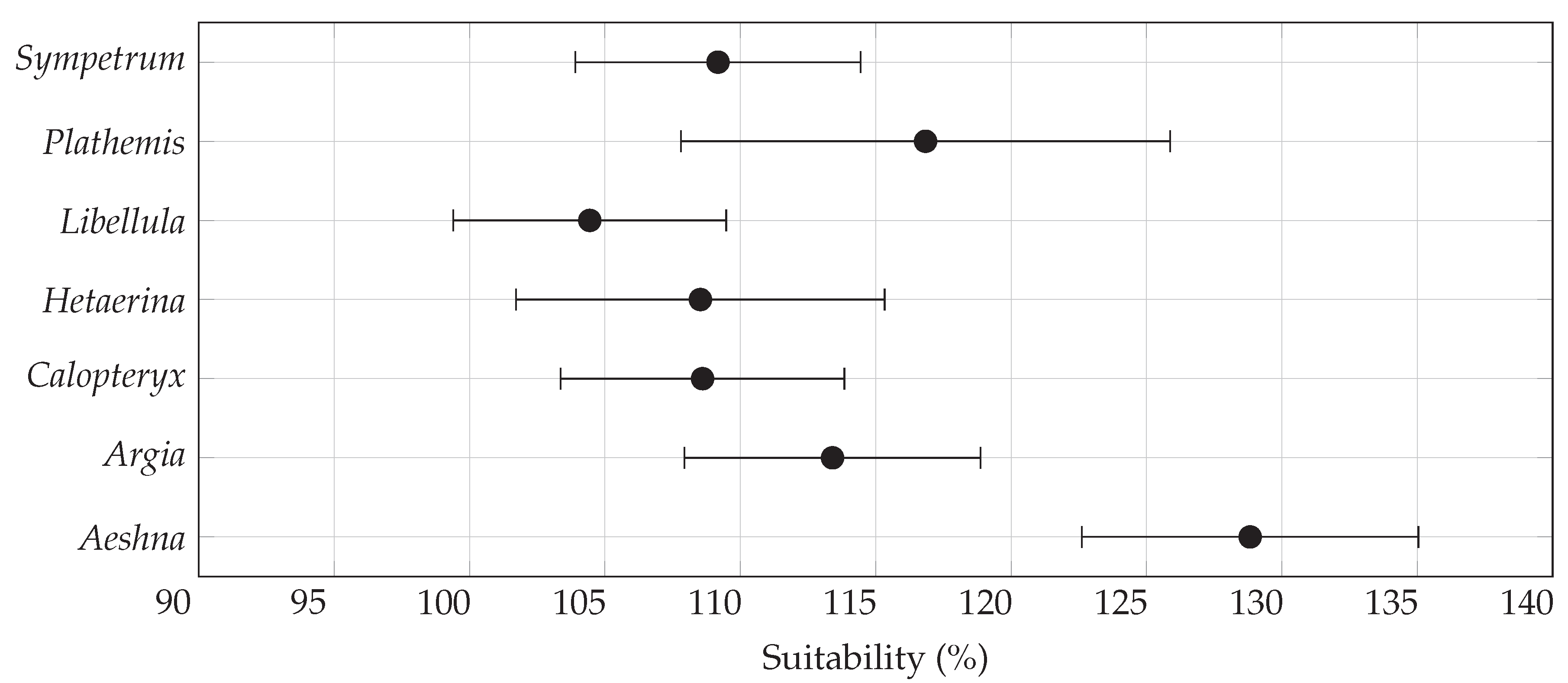
Figure 2.
Marginal means for overall habitat suitability, grouped by genus and SSP. X-axis shows the change in suitability, with 100% representing the baseline scenario; on Y-axis are the seven functional groups.
Figure 2.
Marginal means for overall habitat suitability, grouped by genus and SSP. X-axis shows the change in suitability, with 100% representing the baseline scenario; on Y-axis are the seven functional groups.
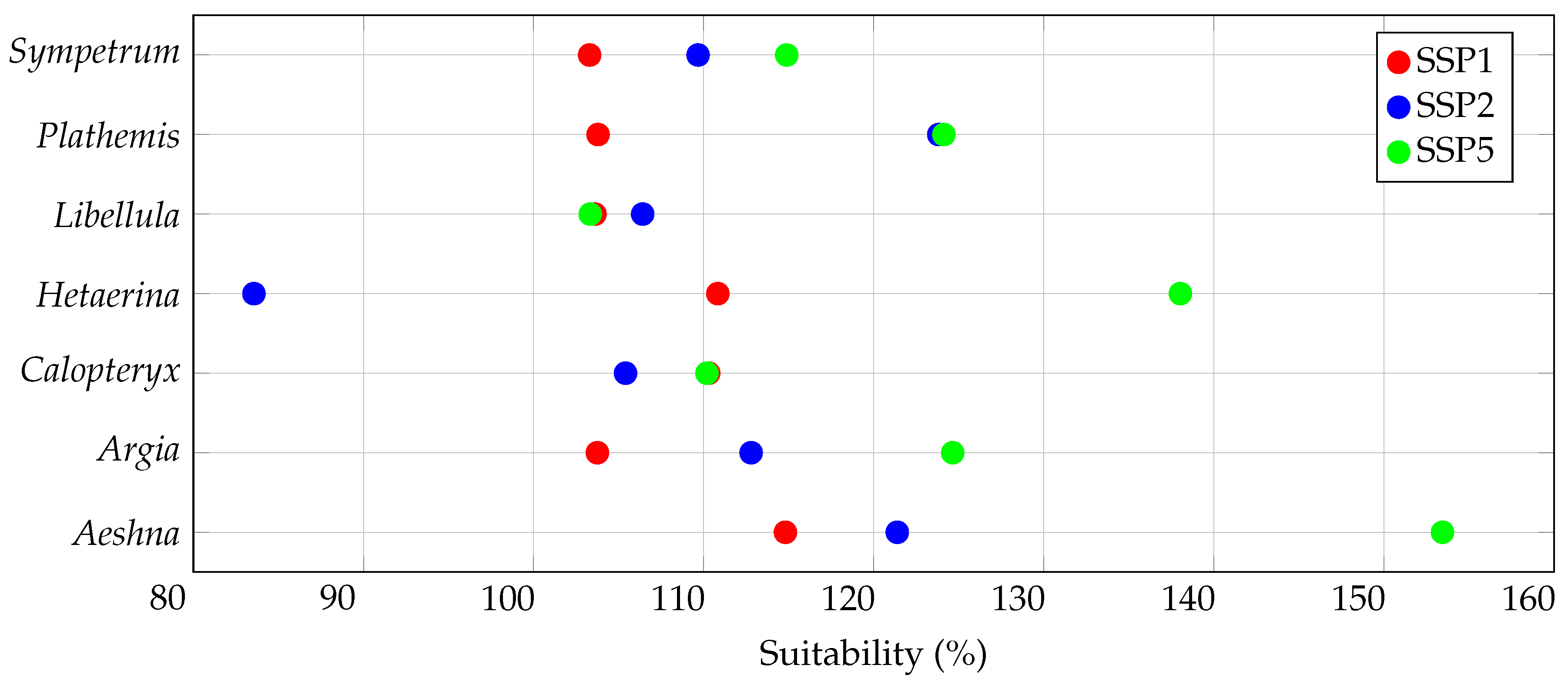
Figure 3.
Marginal means for range size, grouped by genus. X-axis shows the change in range, with 100% representing the baseline scenario; on Y-axis are the seven functional groups.
Figure 3.
Marginal means for range size, grouped by genus. X-axis shows the change in range, with 100% representing the baseline scenario; on Y-axis are the seven functional groups.
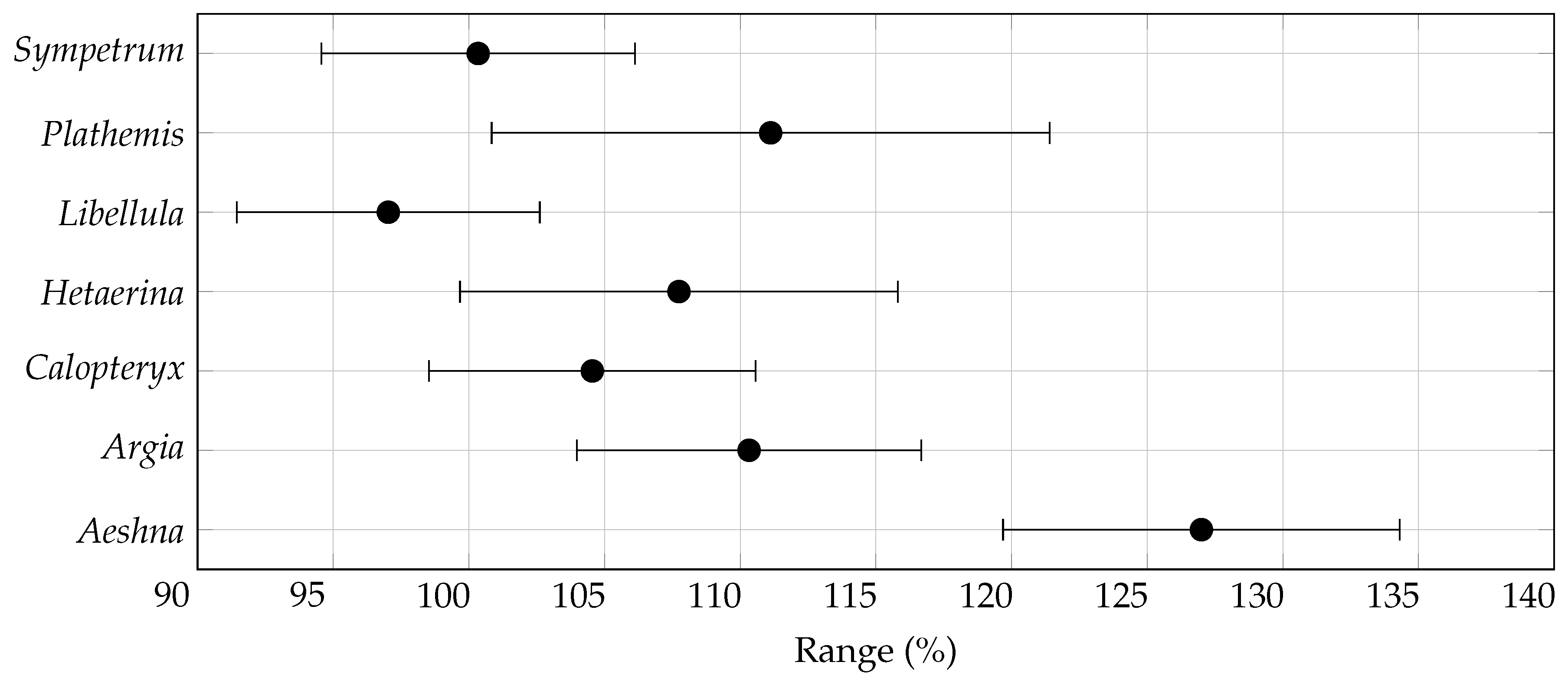
Figure 4.
Marginal means for range size, grouped by genus and SSP. X-axis shows the change in range, with 100% representing the baseline scenario; on Y-axis are the seven functional groups.
Figure 4.
Marginal means for range size, grouped by genus and SSP. X-axis shows the change in range, with 100% representing the baseline scenario; on Y-axis are the seven functional groups.
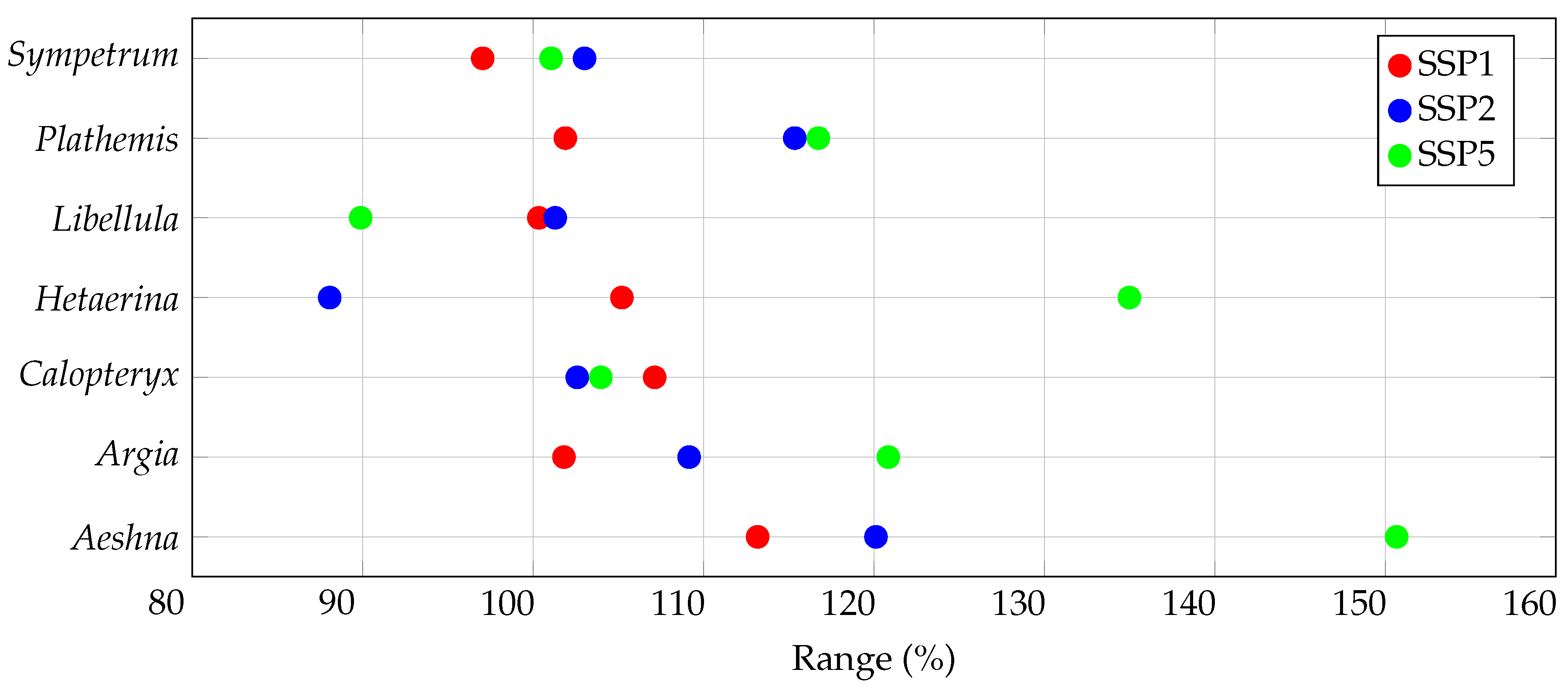
Figure 5.
Marginal means for centroid change, grouped by genus. X-axis shows the change in centroid, with 0 representing the baseline scenario; on Y-axis are the seven functional groups.
Figure 5.
Marginal means for centroid change, grouped by genus. X-axis shows the change in centroid, with 0 representing the baseline scenario; on Y-axis are the seven functional groups.
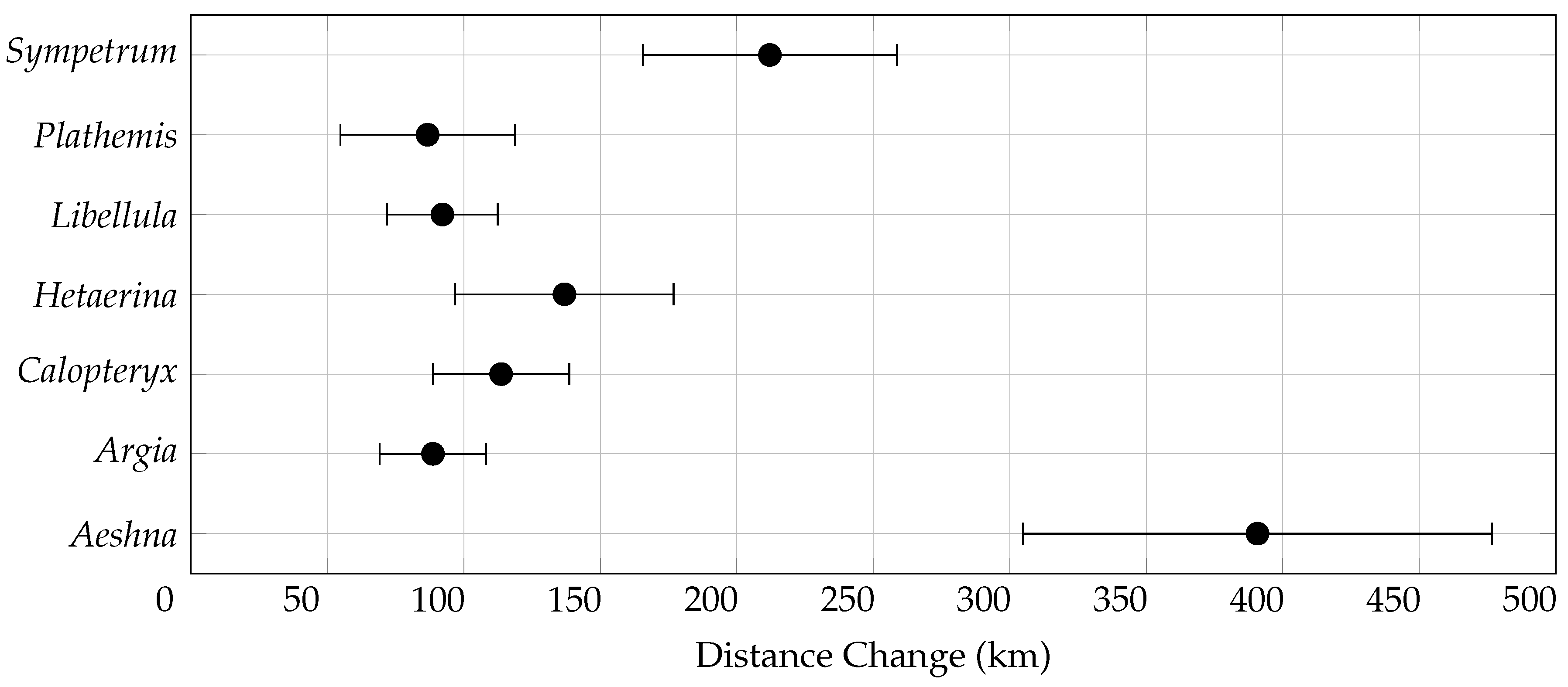
Figure 6.
Marginal means for centroid change, grouped by genus and SSP. X-axis shows the change in centroid, with 0 representing the baseline scenario; on Y-axis are the seven functional groups.
Figure 6.
Marginal means for centroid change, grouped by genus and SSP. X-axis shows the change in centroid, with 0 representing the baseline scenario; on Y-axis are the seven functional groups.
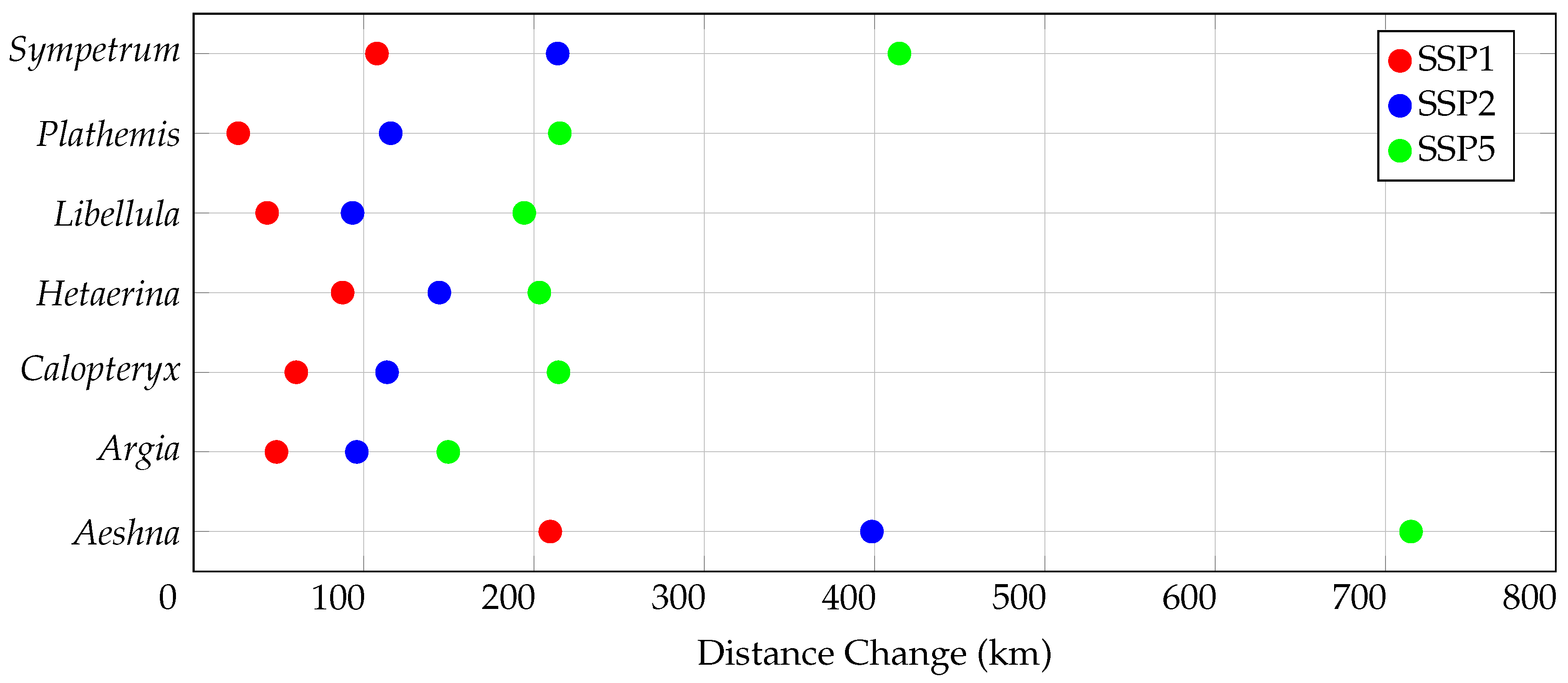
Figure 7.
Permutation importance of environmental variables. See Table 2 for a full list of explanations of variable abbreviations.
Figure 7.
Permutation importance of environmental variables. See Table 2 for a full list of explanations of variable abbreviations.
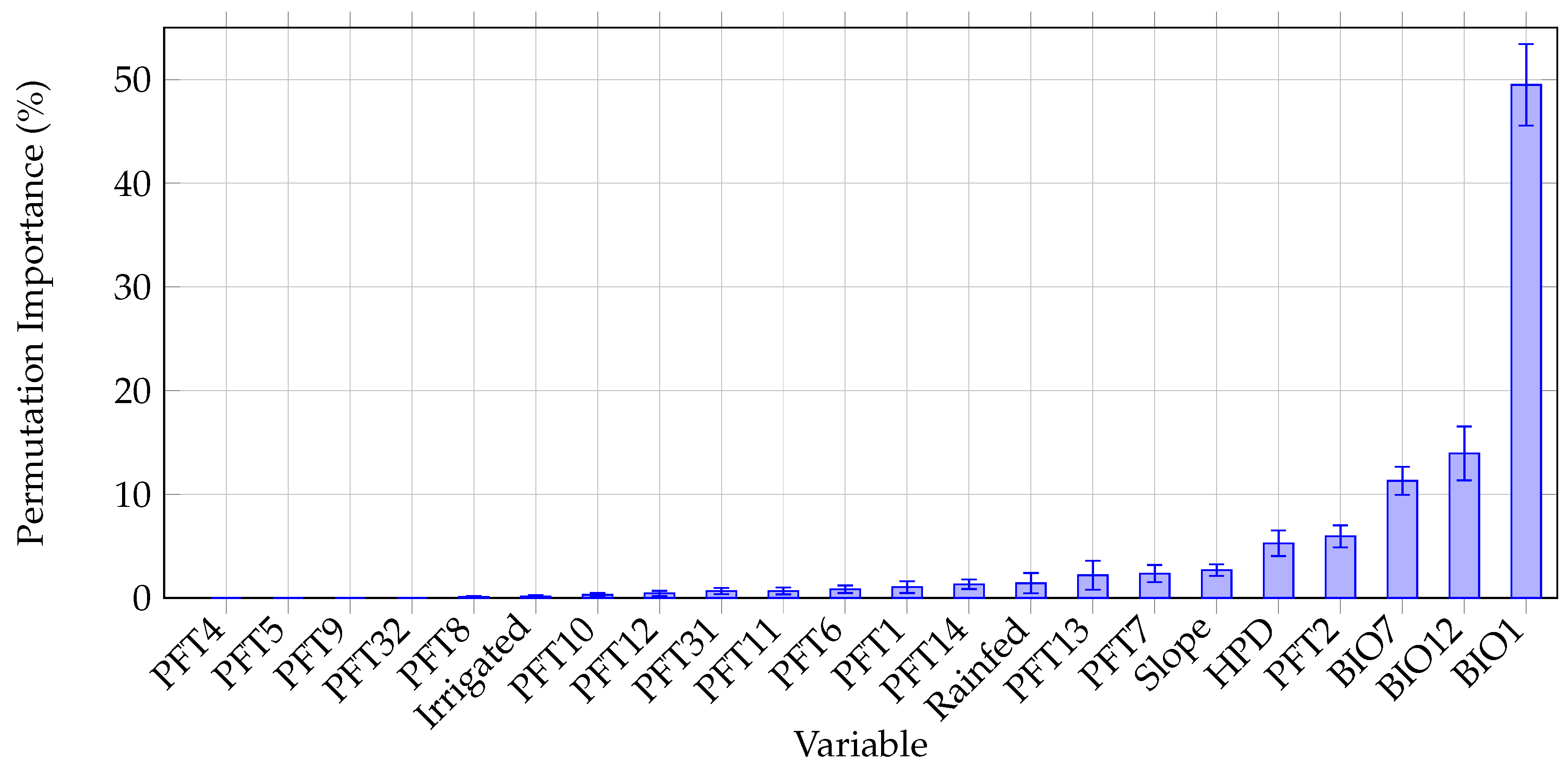
Figure 8.
Case study: predicted distribution of Calopteryx angustipennis in 2020 (baseline; blue), and in 2100 under SSP5 (scenario with the most drastic changes; red). Predicted habitat would move north and fragment into four smaller pieces. Overlay generated from predictions by my models; basemap by Esri [54].
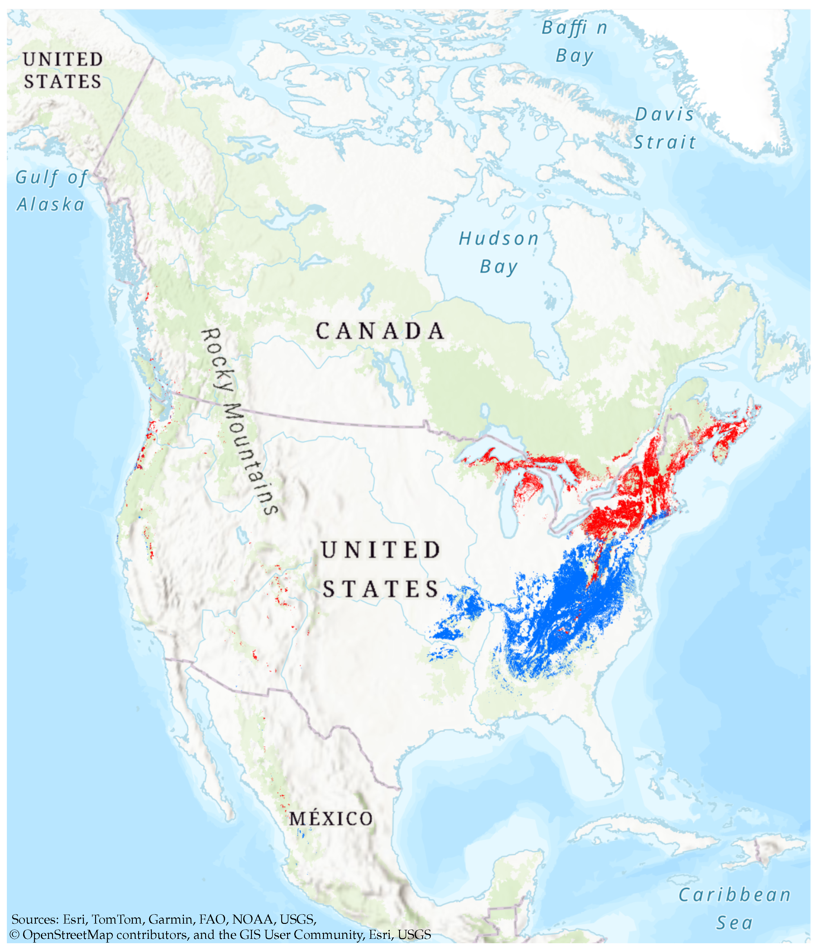
Table 1.
The 30 selected species representing the seven genera and their respective number of records during the period 2015–2025.
Table 1.
The 30 selected species representing the seven genera and their respective number of records during the period 2015–2025.
| Species | Records | Species | Records |
| Aeshna umbrosa | 1,010 | Hetaerina americana | 2,509 |
| Aeshna palmata | 578 | Hetaerina titia | 540 |
| Aeshna canadensis | 496 | Hetaerina vulnerata | 179 |
| Aeshna interrupta | 428 | Libellula luctuosa | 6,393 |
| Aeshna constricta | 291 | Libellula incesta | 5,135 |
| Argia fumipennis | 2,922 | Libellula pulchella | 3,959 |
| Argia apicalis | 2,858 | Libellula vibrans | 2,656 |
| Argia moesta | 2,678 | Libellula cyanea | 1,691 |
| Argia sedula | 1,866 | Plathemis lydia | 8,991 |
| Argia tibialis | 1,614 | Plathemis subornata | 127 |
| Calopteryx maculata | 3,669 | Sympetrum vicinum | 2,880 |
| Calopteryx aequabilis | 514 | Sympetrum corruptum | 2,157 |
| Calopteryx dimidiata | 307 | Sympetrum semicinctum | 1,073 |
| Calopteryx angustipennis | 89 | Sympetrum obtrusum | 876 |
| Calopteryx amata | 72 | Sympetrum ambiguum | 749 |
Table 2.
VIF values for the 22 selected variables. Variables with the prefix “BIO” are bioclimatic, while variables with the prefix “PFT” are plant functional types (land use). “Ndlf” = Needleleaf, “Bdlf” = Broadleaf, “Evgr” = Evergreen, “Dcds” = Deciduous.
Table 2.
VIF values for the 22 selected variables. Variables with the prefix “BIO” are bioclimatic, while variables with the prefix “PFT” are plant functional types (land use). “Ndlf” = Needleleaf, “Bdlf” = Broadleaf, “Evgr” = Evergreen, “Dcds” = Deciduous.
| Variables | VIF | Variables | VIF |
| BIO1 (Annual Mean Temperature) | 11.350 | PFT10 (Bdlf Dcds Shrub Temperate) | 4.303 |
| BIO7 (Temperature Annual Range) | 5.164 | PFT11 (Bdlf Dcds Shrub Boreal) | 7.013 |
| BIO12 (Annual Precipitation) | 3.031 | PFT12 (C3 Arctic) | 3.776 |
| PFT1 (Ndlf Evgr Tree Temperate) | 5.136 | PFT13 (C3 Grass) | 11.423 |
| PFT2 (Ndlf Evgr Tree Boreal) | 20.126 | PFT14 (C4 Grass) | 6.675 |
| PFT4 (Bdlf Evgr Tree Tropical) | 3.705 | PFT31 (Urban) | 1.352 |
| PFT5 (Bdlf Evgr Tree Temperate) | 1.389 | PFT32 (Barren) | 5.640 |
| PFT6 (Bdlf Dcds Tree Tropical) | 2.528 | PFT Rainfed Crops Cumulative | 5.035 |
| PFT7 (Bdlf Dcds Tree Temperate) | 3.566 | PFT Irrigated Crops Cumulative | 1.497 |
| PFT8 (Bdlf Dcds Tree Boreal) | 1.798 | HPD (Human Population Density) | 1.028 |
| PFT9 (Bdlf Evgr Shrub Temperate) | 1.011 | Slope | 1.377 |
Disclaimer/Publisher’s Note: The statements, opinions and data contained in all publications are solely those of the individual author(s) and contributor(s) and not of MDPI and/or the editor(s). MDPI and/or the editor(s) disclaim responsibility for any injury to people or property resulting from any ideas, methods, instructions or products referred to in the content. |
© 2025 by the author. Licensee MDPI, Basel, Switzerland. This article is an open access article distributed under the terms and conditions of the Creative Commons Attribution (CC BY) license (http://creativecommons.org/licenses/by/4.0/).
Copyright: This open access article is published under a Creative Commons CC BY 4.0 license, which permit the free download, distribution, and reuse, provided that the author and preprint are cited in any reuse.


