
Submitted:
23 October 2025
Posted:
24 October 2025
You are already at the latest version
Abstract
Supercritical carbon dioxide (sCO2) is characterized by low viscosity and a peak in specific heat capacity near the pseudo--critical point, making it a promising coolant for microelectronics cooling. However, most existing sCO2 test rigs are designed for large-scale thermodynamic cycle studies and lack the capability for controlled, localized heat transfer measurements in small channels. This work presents CO2-SASS (Scientific Assessment of heat transfer in the Supercritical State), a modular, high-pressure test rig designed to measure local heat transfer coefficients and pressure drops in stainless-steel tubes with diameters in the order of 1-3 mm. The system provides independent control of pressure, mass flow and heating, with direct local wall and fluid temperature as well as precise absolute and differential pressure measurements. Particular emphasis is placed on high-accuracy temperature acquisition, including individual thermocouple calibration and cold-junction bias correction. A detailed uncertainty analysis highlights the dominant role of temperature measurement accuracy, especially for small wall-fluid temperature differences near the pseudo-critical point.
Keywords:
carbon dioxide
; cooling
; supercritical
; microelectronics
; heat transfer coefficient
; pressure drop
; experimental
; small channel
1. Introduction
In the field of thermal management, supercritical carbon dioxide (sCO2) has gained significant attention as a promising coolant for various applications, particularly in high performance heat exchangers and microelectronics cooling. The favorable thermophysical properties of sCO2—such as its high density, low viscosity and large specific heat capacity near the critical point—enable the development of compact heat exchangers, significantly reducing the size of thermal systems while maintaining performance [1]. This compactness and thermal efficiency make sCO2 particularly applicable in microelectronics cooling, where space constraints and high heat fluxes are common. A preliminary study by ElGenk demonstrated its viability in such applications [2], where high heat transfer coefficients were reported in an additively manufactured cold plate. Furthermore, Fronk and Rattner [3] discussed the potential use of sCO2 as the working fluid for high-flux thermal management. They highlighted the need for key research before its practical application, including solving the uncertainty in supercritical heat transfer coefficients and characterizing the heat transfer effects in small channels.
As most of the research in supercritical fluids throughout history has been focused on nuclear reactor cooling applications, the studies so far have had very different conditions compared to the typical ones in microelectronics cooling, being the most important one the pipe diameter. For CO2, most studies have measured heat transfer coefficients in heated pipes with sizes ranging 4 to 10 mm; see [4,5,6]. Only two studies have reported convective heat transfer coefficients in pipe sizes below 2 mm[7,8] and have not provided enough conclusive data to properly understand the effect of different system variables: inlet temperature, hydraulic diameter, heat flux. Additionally, they only reported heat transfer coefficient and missed to comment on the pressure drop results, although their test rigs did measure them.
The potential of supercritical CO2 as a coolant arises from the change in its thermophysical properties around the critical region. Figure 1 shows the variation of density, heat capacity, viscosity, and thermal conductivity with temperature at different pressures. The critical point of CO2 is at 73.8 bar. Below this value, at subcritical conditions, an isobaric addition of heat into a system induces boiling, and therefore the coexistence of liquid and vapor phases. Above it, two distinct phases can no longer coexist and the fluid instead behaves as a single phase with properties that combine features of both liquids and gases: a liquid-like density, which enhances convective heat transfer per unit volume, and a gas-like viscosity, which reduces pumping power requirements.
A particularly interesting feature occurs near the so-called pseudo–critical point 1, where the specific heat capacity exhibits a pronounced peak. In this regime, large amounts of heat can be absorbed with only a modest increase in fluid temperature. However, this sharp dependence on pressure and temperature also explains why cooling with supercritical fluids remains difficult to characterize. Small variations in operating conditions strongly affect the heat transfer response, and existing correlations often fail to reproduce experimental data consistently. Up to date, no universally applicable correlation for a given geometry has been established [10], highlighting the need for systematic parametric measurements.
This lack of consistent correlations is closely linked to the extreme sensitivity of heat transfer coefficients near the pseudo-critical region. Even minor deviations in measured temperature or pressure can cause large variations in the calculated values. As a result, reported data in the literature often differ significantly from one another [11].
Moreover, the experimental tools available to explore the potential of sCO2 as a refrigerant remain limited. Most existing test rigs are developed for applications such as thermodynamic cycle optimization, turbomachinery validation, or compact heat exchanger design, often focusing on integral system performance rather than localized thermal behavior. These setups typically operate at high total flow rates in larger channels, and are not designed to study the localized heat transfer behavior at the high mass fluxes and small hydraulic diameters relevant to microelectronics-scale applications. As a result, they lack the flexibility to conduct controlled, repeatable parametric studies of sCO2 heat transfer under conditions relevant to small-scale, high-flux thermal management.
To address this gap, a modular test rig has been designed and constructed in order to investigate sCO2 heat transfer across a wide range of flow rates, pressures, and heat fluxes under conditions relevant to microelectronics cooling. The system enables direct measurement of local wall and fluid temperatures, as well as pressure drop across a small-diameter test section (in the range of 1 to 3 mm), additionally offering the flexibility to adjust layout, inlet conditions and sensor positioning for high-resolution thermal characterization.
Finally, the operating conditions of the test rig have been selected to enable direct comparison between subcritical and supercritical regimes. By using the same instrumentation and equipment, the setup can replicate both evaporative heat transfer below the critical point and single-phase heat transfer above it. This unique capability allows systematic investigation of the fundamental differences between the two regimes, which remain poorly understood and insufficiently documented in the literature [5].
2. Design
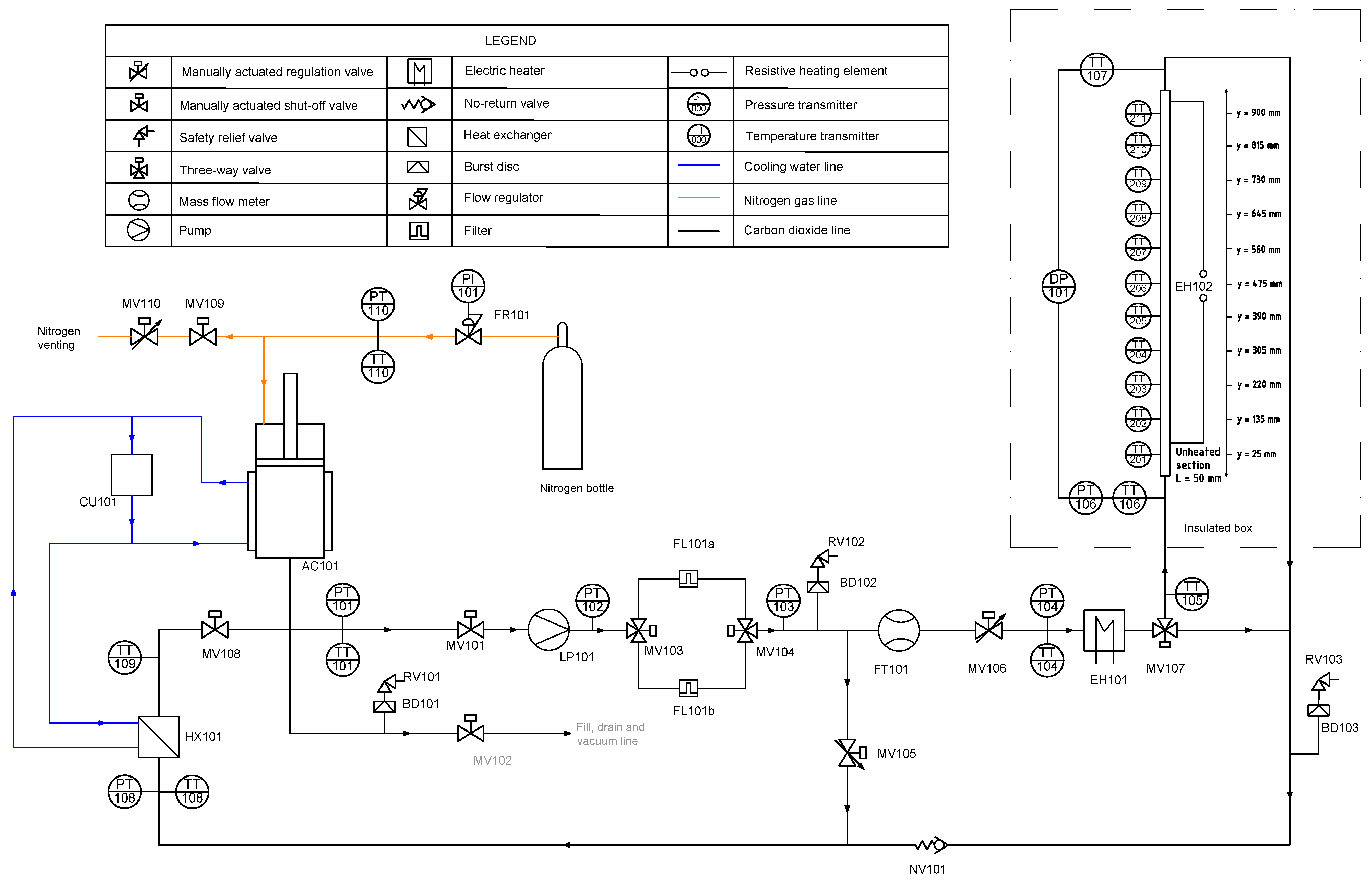
The test rig was designed to investigate sCO2 heat transfer in a capillary geometry, with precise control over pressure, mass flow rate, heat input, and flow orientation. The process and instrumentation diagram (P&ID) is shown in Figure 3. A detailed description is included in this section, as well as the Bill of Materials (Table 2). As this section contains all the necessary information respective to hardware, Table 1 lists the sensor uncertainties, while their specific calculation methods are detailed further in 6. Operating instructions are included in Section 4.
Carbon dioxide is pressurized by using nitrogen gas inside a combined metal bellows–piston accumulator (AC101), equipped with a cooling coil. The bellows and piston sections are mechanically coupled, enabling a maximum displacement volume of 3 liters. This configuration allows dynamic pressure regulation while fully isolating the nitrogen and CO2 sides, preventing any cross-contamination.
The accumulator serves as the system’s pressure setpoint controller and maintains pressures in the 50–120 bar range. It also functions as a thermal buffer, stabilizing the stored liquid by accommodating volume changes and avoiding pressure spikes. Although the role of the accumulator is functionally similar to that of a commercial hydraulic accumulator, a custom design was implemented to ensure long-term safety and purity of the working fluid. Several alternatives were considered, including piston, bladder/diaphragm, and bellows accumulators. However, while piston and bladder types could allow long-term nitrogen permeation, metal bellows are highly sensitive to overpressure. In this regard, given the long-term nature of the experimental program and the involvement of multiple operators, a fail-safe configuration was prioritized. This led to the selection of a coupled piston–bellows accumulator, which combines the contamination-free characteristics of a bellows with the mechanical robustness of a piston. While the exact internal configuration of the current accumulator is proprietary, equivalent functionality could be achieved using a coupled system of two commercially available accumulators: one charged with a high pressure gas and one containing CO2, mechanically linked to transmit pressure without fluid contact.
Alternatively, if maintaining strict fluid purity is essential, for example, in experiments targeting precise heat transfer coefficient measurements, a single metal bellows accumulator can be used, provided it is paired with a carefully designed control strategy to manage system filling and pressure adjustments. On the other hand, for less demanding applications, where a small degree of nitrogen–CO2 cross-contamination is acceptable, a piston accumulator with a PTFE seal may offer a simpler and more cost-effective solution.
Downstream of the accumulator, the fluid is circulated by a magnetically driven rotary vane pump (LP101), controlled by a variable frequency drive (VFD). As this is a dry pump, the continuously rotating cartridge (housing the vanes) is subject to wear. This means that clearances gradually increase and the pump is expected to lose head, therefore flow performance over time. Absolute pressure is measured before and after the pump to monitor this degradation. An inline filter (FL101) removes debris immediately downstream. To allow for continuous operation without emptying the test rig, two filters in parallel are installed. With time, the filter will become saturated with debris and have to be cleaned. An absolute pressure sensor has been installed directly downstream to detect increasing pressure drop and switch between filters. To protect the pump and maintain stable operation, a bypass valve (MV101) is installed directly downstream. This ensures continuous circulation even when flow demand is low, avoiding conditions where the pump would otherwise operate at insufficient flow rates.
The remaining mass flow rate is measured by a Coriolis flow meter (FT101), which is the actual flow passing through the test section. In this section of the rig, two manual valves (MV106 and MV107) can be used characterizing and diagnosing the pump. During normal operation, the regulation valve is kept fully open and the three-way valve always points at the test section. The fluid is then preheated using an electric heater (EH101) before entering the test section. Temperatures are measured up and downstream the electric heater to monitor its correct operation.
After this, the fluid enters the test section, which consists of a 1 m long stainless steel (304L) capillary with an inner diameter of 1.00 mm and outer diameter of 1.59 mm. Resistive heating is applied via clamped electrodes (EH102), powered by a DC power supply. To avoid parasitic current leakage, dielectric fittings are placed at both ends of the test section. Up and downstream adiabatic segments ensure flow development prior to the heated zone.
Wall temperatures are measured at eleven points along the heated pipe using K-type thermocouples directly attached to the outer surface. The sensors are calibrated as described in Section 5.2 and installed afterwards using epoxy steel putty and thermal paste. In-fluid PT-100 temperature sensors are also installed at both the inlet and outlet of the test section, while absolute pressure is measured only at the inlet. Instead of direct pressure measurement at the outlet, a differential pressure sensor measures pressure drop along the tested area. After the test section, the fluid passes through a compact heat exchanger, cooled by a chiller unit (CU101), before returning to AC101 to complete the loop.
The entire test section is mounted within an insulated, tiltable support frame, enabling experiments at various flow orientations without modifying instrumentation. The test section can also be easily removed, so that different types of pipes or configurations can be tested using the same rig.

Table 1.
System variable sensors nomenclature, type of sensor and their uncertainties.
| Measured variable | Designator | Number | Sensor type | Derived uncertainty |
| Absolute pressure | PT | 101-110 | Piezoresistive sensor | 0.2 bar |
| Differential pressure | DP | 201 | Capacitive sensor | 0.003 bar |
| Mass flow | FT | 101 | Coriolis flow meter | 0.04 g/s |
| Fluid temperature | TT | 101-110 | PT100 | 0.05 K (after calibration) |
| Wall temperature | TT | 201-211 | Type K thermocouple | 0.07 K (after calibration) |
Table 2.
Bill of Materials (BOM) for CO2-SASS.
| Quantity | Component | Source / Manufacturer | Material type | Approx. cost/unit (EUR) |
| 1 | Piston–bellows accumulator (AC101) | HYDAC (bespoke design) | Stainless steel | Upon request |
| 3 | High-purity bursting disc (BD101) | Schlesinger, Type U | Stainless steel | 500 |
| 1 | Chiller unit (CU101) | Van der Heijden, VDH5000A | Mixed metals/plastics | 15000 |
| 1 | Electric heater (EH101) | WATLOW, CAST X-500 | Stainless steel / aluminium | 1500 |
| 2 | Inline filter (FL101) | LEWA, FMI2, 3 µm | Stainless steel | 600 |
| 1 | Pressure regulator (FR101) | Gloor, 200 bar | Stainless steel | 500 |
| 1 | Plate heat exchanger (HX101) | SWEP, B4THx30 | Stainless steel | 160 |
| 1 | Rotary vane pump (LP101) | M-PUMPS, VA01 MODULAR 2S | Stainless steel | 19000 |
| 1 | High-pressure relief valve (RV101) | Parker, HPRV | Stainless steel | 600 |
| 10 | Manual valves (MV, shut-off) | Swagelok, 43G Series | Stainless steel | 160 |
| 3 | Manual valves (MV, regulation) | Swagelok, 31 Series | Stainless steel | 150 |
| 10 | PT100 in-fluid temperature sensors | Rodax, Class A, 4-wire | Platinum RTD | 120 |
| 11 | K-type wall thermocouples | Roessel Messtechnik | NiCr/NiAl | 14 |
| 7 | Absolute pressure sensors (PT1xx) | Keller AG, 23SX | Stainless steel | 380 |
| 1 | Differential pressure transmitter | Endress+Hauser, PMD75B | Stainless steel | 2800 |
| 1 | Thermal insulation sheet | RS Components | Glass wool | 120 |
| 1 | Thermal insulation | Armacell, Armaflex | Elastomer foam | Upon request |
| - | Fittings | Swagelok | Stainless steel | Upon request |
| - | Structural aluminium extruded profiles | Aldiance | Aluminium | Upon request |
Figure 2.
Images of the CO2-SASS experimental system.
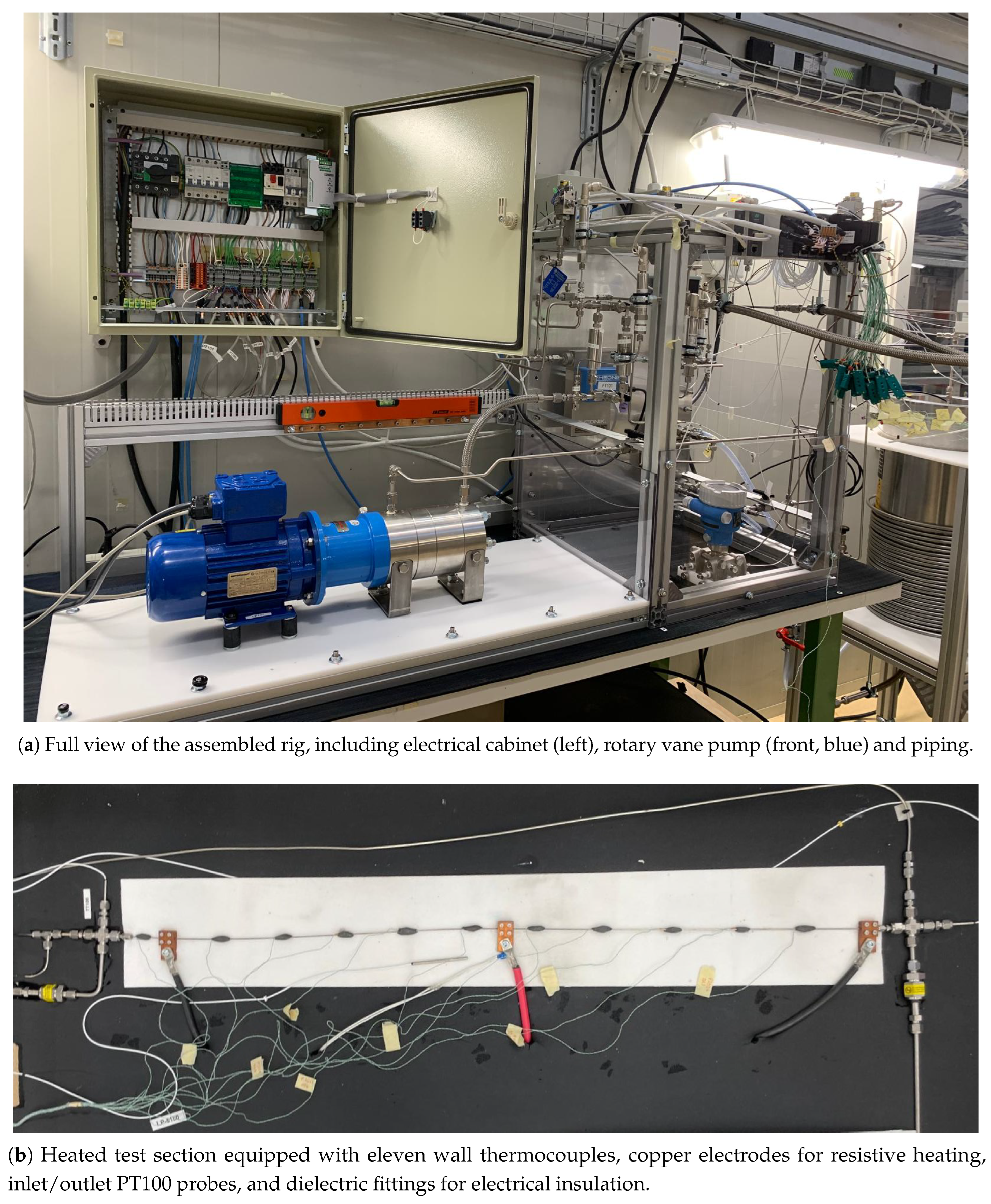
Figure 3.
Piping and instrumentation diagram (P&ID) of the CO2-SASS setup. All major components are shown, including pressure and temperature sensors (PT, TT respectively), heaters, valves, and flow elements.
Figure 3.
Piping and instrumentation diagram (P&ID) of the CO2-SASS setup. All major components are shown, including pressure and temperature sensors (PT, TT respectively), heaters, valves, and flow elements.
Data acquisition and control are handled using National Instruments (NI) hardware and custom LabVIEW-based software for process control and logging. Process signals and parameters are collected in a cDAQ-9178, which forms the heart of the monitoring system. Figure 4 summarizes the modules and their associated signal types. While a detailed explanation of each module is omitted here for brevity, except for the uncertainty derivation discussed in Section 5.2, interested readers may refer to the figure and manufacturer website for further insight.
3. Build Instructions
The construction of the CO2-SASS rig follows directly from the design choices described in Section 2. The steps below outline the assembly process in sufficient detail to enable reproduction.
- Frame and structural support: Assemble the main support frame using extruded aluminium profiles. The frame must be dimensioned to accommodate the accumulator, pump, filters, heat exchanger, and test section. Install an insulated tiltable mount for the test section to allow experiments at different orientations, if desired.
- Piping: Use stainless steel 316L tubing with 4 mm inner diameter and 6 mm outer diameter for the main CO2 loop. For the pressure sensor lines, use in. OD stainless steel tubing. Connect all tubing with Swagelok VCR fittings to facilitate repeated assembly and disassembly without loss of sealing performance.
- Accumulator (AC101): Install the piston–bellows accumulator upstream of the pump. Connect one side to the CO2 loop and the other to the nitrogen regulator (FR101) for pressure control. Ensure a cooling coil is fitted around the accumulator body for thermal stabilization.
- Pump and filters: Mount the magnetically driven rotary vane pump (LP101) downstream of the accumulator. Install a bypass valve (MV105) directly after the pump outlet to protect against low-flow conditions. Place two inline filters (FL101) in parallel, with valves to isolate each filter for maintenance. Connect an absolute pressure sensor downstream of the filters to monitor clogging.
- Flow and heating section: Install the Coriolis flow meter (FT101) downstream of the filters. Place the electric preheater (EH101) after the flow meter. Install manual valves MV106 and MV107 to allow pump characterization during commissioning.
- Test section: Mount the 1 m stainless steel capillary (1.00 mm ID, 1.59 mm OD) within the insulated tiltable support. Attach copper electrodes for resistive heating (EH102) at both ends, ensuring dielectric fittings prevent leakage currents. Apply thermal paste and epoxy steel putty to fix eleven K-type thermocouples (TT201–TT211) along the outer wall. Install PT100 probes at the inlet and outlet, and connect the differential pressure transmitter to the test section ends.
- Cooling section: Route the outlet flow through the plate heat exchanger (HX101), cooled by the chiller unit (CU101). Connect the return line to the accumulator to close the loop.
- Instrumentation and control: Connect all pressure, temperature, and flow sensors to the NI cDAQ-9178 chassis, using the modules specified in Figure 4. Wire the heaters and pump drive to the control cabinet. Install safety devices, including the high-pressure relief valve (RV101) and bursting discs (BD101), at appropriate positions.
- Insulation: Apply glass wool insulation sheets around the test section and thermally insulating elastomer foam around the tubing to minimize heat loss and ensure stable thermal conditions.
All parts listed in Table 2 are commercially available and can be assembled using standard laboratory tools. Deviations such as larger tubing diameters or alternative valves may be implemented depending on the target flow rate and available equipment.
4. Operating Instructions
4.1. Filling the System
The system must be fully vacuumed before charging it with carbon dioxide. A vacuum pump is connected to MV102 and left for one hour, having all the rest of the valves open to properly vent the entirety of the setup of any air. Afterwards, a bottle containing two-phase carbon dioxide (quality 48), equipped with a pressure regulator, is placed on a scale and connected to the same valve. The line is then filled with liquid carbon dioxide while keeping MV102 in closed position. This step ensures that there is no air going inside the setup from the hose. The scale is then zeroed.
MV102 is then opened again to allow carbon dioxide to flow inside the system. Once stabilized, the regulator is further opened to increase the pressure on the system side. The pressure is firstly set to 20 bar and allowed to equalize for 15 minutes. Then, pressure is increased in 10 bar increments and allowed to rest. Finally, when the pressure of the bottle has been reached, the system is allowed to stabilize. MV102 is closed when the scale measurement has reached kg.
The fill pressure will be the maximum pressure attainable with the CO2 bottle, which will depend on the mass contained and the ambient temperature. To achieve higher pressures inside the rig, nitrogen has to be filled on the other side of the accumulator. For this, FR101 must be opened to pressurize with nitrogen gas. A very precise control of the system pressure can be achieved when working together with FR101, to allow nitrogen in the system, and MV110, to vent excess pressure.
4.2. Steady Operation
To operate the test rig, firstly an initial operating pressure is chosen and set with FR101. The pump LP101 can then be started to set a stable operating condition. After equalization of temperatures, depending on the initial state, the pressure will have changed and can be readjusted to its desired value in PT106 by means of opening MV110. The mass flow can also be adjusted to its value of interest using MV105. Heaters EH101 and/or EH102 will be then used depending on the nature of the tests to be carried out. This is done by means of the LabVIEW software, which can be found in the Supplementary Materials.
A steady state point is considered only when the temperature variation at each sensor remains within K for a period of five minutes, ensuring negligible transient effects. This threshold is well below the absolute uncertainty of the temperature sensors and confirms thermal stability during each measurement point. At the moment, due to the nature of the software, the acquisition rate is fixed at 1 Hz; however, it is planned to remove this constraint in the future.
5. Fundamentals
5.1. Convective Heat Transfer Coefficient
In convective heat transfer, the local heat transfer coefficient represents the rate of heat transfer per unit area and per unit temperature difference between the surface and the fluid. This coefficient is the most fundamental parameter of convective heat transfer, while at the same time its derivation is highly indirect: the value is obtained after a long chain of measurements and is therefore heavily affected by errors. The SI units are and its value can be experimentally derived as:
Where is the local heat flux, obtained from the heat flow (Q) per unit area:
calculated by evaluating the enthalpy rise of the working fluid across the test section.
Here, is the measured mass flow rate, and , are the specific enthalpies at the inlet and outlet of the heated section, respectively. Inlet enthalpy is calculated using directly measured pressure and temperature values, while outlet enthalpy is obtained from the outlet temperature and a pressure value determined as , with measured across the entire test section (DP101 in Figure 3).
5.2. General Uncertainty Calculation
The derived uncertainties for all measured variables are obtained using the standard uncertainty propagation method based on a first-order Taylor series expansion:
In this formula, is the overall uncertainty of the result variable y, which is affected by the uncertainties of the other variables it depends on. The terms are called sensitivity coefficients and show how much the result changes when each variable changes.
This approach assumes that the input variables are uncorrelated. In cases where strong correlations are present, a full covariance matrix is required. All reported uncertainties correspond to one standard deviation (1), unless otherwise noted.
In practical terms, when the measured variables are not strongly dependent on one another, the total uncertainty is simply the square root of the sum of the squares of the individual uncertainties.
6. System Calibration and Measurement Uncertainty
Wall temperatures are universally measured using thermocouples when the pipe size is below 2 mm in supercritical systems2. However, the methods for their placement and signal interpretation vary significantly across studies, as there is no established standard. In some cases, thermocouples are sheathed and embedded in a copper block surrounding the heated section [8]. In other cases, thermocouples are directly soldered or spot-welded to the pipe wall [4], which reduces thermal mass and contact resistances but is not feasible in thin-walled tubes.
Moreover, a key element that is rarely addressed in detail when using thermocouples is the treatment of the cold junction. While modern acquisition systems offer automatic cold junction compensation, the typical accuracy of these modules (cold junction temperature measurement accuracy) is on the order of ±0.25 K to K. Any errors in reading the cold junction temperature will contribute directly to errors in the final temperature measurement if one considers Taylor’s propagation of uncertainty. Some studies report thermocouple uncertainties below this limit, without clarifying the reference method or compensation strategy used. Whether this is due to post-calibration, unreported ice bath references, or optimistic estimates remains unclear. The lack of transparent discussion on this topic further complicates the comparison of heat transfer data across the literature and could be one of the main contributors to the scattered distribution of the data at supercritical conditions.
All temperature measurements in CO2-SASS have been referenced to the ITS-90 temperature scale.
6.1. Thermocouples
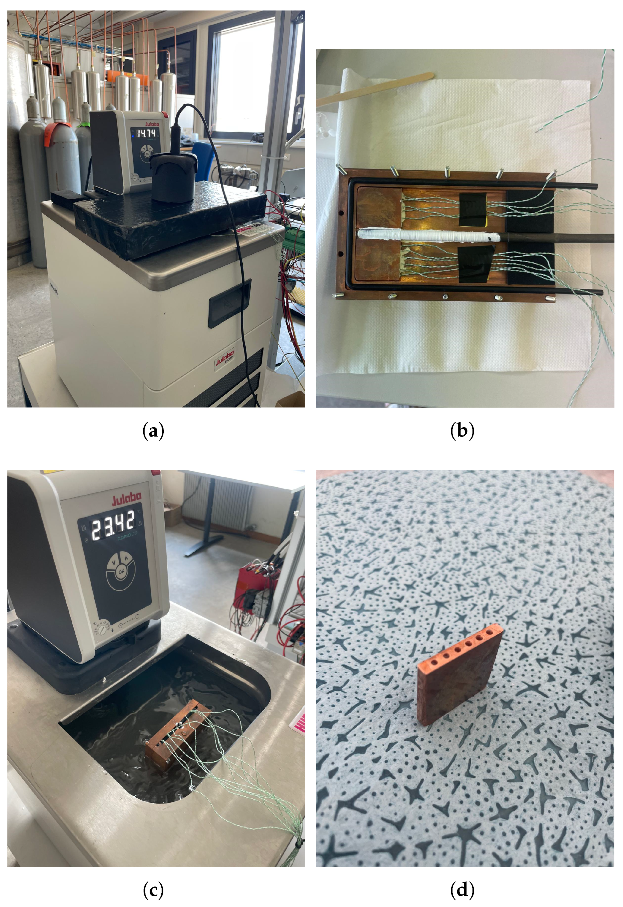
Type K thermocouples were used for wall temperature measurements. To characterize each individual thermocouple in the DAQ chain, they were embedded in an in-house built copper block, submerged in a temperature-controlled bath. An insert was machined to tightly contain the probes, which were covered in electrical insulation beforehand and placed inside the insert, together with thermal paste. Figure 5 shows different steps and equipment used for the calibration. A range of temperatures from 0 to 100 oC was covered, in intervals of 10 oC. The voltage measured by each thermocouple was compared to that of a Fluke SPRT (Standard Platinum Resistance Thermometer) embedded in the same copper block, at a similar height. Voltage signals were acquired using NI-9214 modules. The uncertainty of the temperature signal in this case includes sensor tolerance, thermoelectric voltage nonlinearity, and cold junction error.
To correct systematic measurement bias, a calibration equation was obtained for each thermocouple. The problem of thermocouples is that one can get as precise as the cold junction can get, and this can really spoil the whole process of calibration. To counter this, the cold junction was calibrated with a probe placed in an ice bath at the same time as the rest of the sensors. The ice bath was achieved by filling a container with crushed ice and covering the volume with water, as specified by the National Institute of Standards and Technology [12]. The mixture was then mixed and let sit inside a polystyrene box for some seconds right before starting the recording via the software for data acquisition. This was only performed when the temperature of the probes inside the copper block were considered stable.
This correction ensures consistency with the ice bath calibration and improves measurement accuracy by compensating for the cold junction bias. However, having an ice bathconstantly ready and available during an entire data campaign could result quite impractical. For the first results of the rig, a method was followed so that the ice bath was prepared once per day. This procedure assumes that the cold junction temperature remained stable during the testing time, which is valid considering that the temperature in the laboratory did not change significantly from the morning to the afternoon.
In practice, the calibration using the electronic cold junction will be used for all thermocouple measurements, due to its practicality during continuous operation. The ice bath is instead prepared once per day to evaluate the cold junction bias, which is then treated as a constant voltage correction (typically mV) applied to all measurements of that day. Therefore, the ice bath is not used to generate a separate calibration curve, but to correct the electronic CJC-based calibration for systematic error once per day.
The rest of the components of the wall temperature measurement were the uncertainty of the polynomial conversion ( K), the voltage measurement uncertainty of the DAQ module ( K), the uncertainty of the SPRT, ( K) and its readout ( K). These, combined with the regression uncertainty and inserted into Equation 5.2 result in an uncertainty of K.
The calibration procedure is included in Appendix A.
Figure 5.
Steps and equipment used for the calibration of thermocouples. (a) Chiller unit used in the calibration setup; (b) Copper block used to hold sensors; (c) Copper block submerged in temperature-controlled bath; (d) Small copper insert for thermocouple positioning.
Figure 5.
Steps and equipment used for the calibration of thermocouples. (a) Chiller unit used in the calibration setup; (b) Copper block used to hold sensors; (c) Copper block submerged in temperature-controlled bath; (d) Small copper insert for thermocouple positioning.
6.2. PT100
PT100 resistance temperature detectors (RTDs) are used to measure fluid temperatures. The resistance is acquired using NI 9216 and 9217 modules. The uncertainty was derived considering the calibration error and DAQ module resolution.
The calibration curve of each sensor was obtained following the ITS-90 standard for PT100. The calibration process was carried out in a controlled temperature bath set to a series of fixed setpoints spanning the range from 0oC to 100oC. Additionally, measurements at the triple point of water (TPW) were included to provide an absolute reference.
For each setpoint, sensor resistances and the Fluke SPRT reference temperature were recorded simultaneously using a LabVIEW script.
The procedure for the application of the ITS-90 is included in Appendix B.
The total resulting error of the PT100 calibration is K. Combining this with the DAQ card error ( K) and the SPRT and readout error, with the same values used for the thermocouples, results in a total maximum error of K for the fluid temperature.
6.3. Pressures
Absolute and differential pressures were measured using piezoresistive and capacitive sensors. The accuracy of the absolute pressure measurement is a function of the measured value, and it is reported by the manufacturer as . Considering that the measurement range for the sensors on the CO2 side is 0-160 bar, the maximum absolute error is bar. For the nitrogen side, the sensor has a higher range, up to 200 bar, resulting in an absolute error of bar.
The differential pressure sensor has an accuracy of . Being the maximum value 3 bar, this results in bar absolute error.
The error of the acquisition card NI9203 is given by the manufacturer and results in mA. Combining this with the individual sensor sensitivities and adding it to the sensor error calculation results in:
- CO2 absolute sensors: bar.
- N2 absolute sensors: bar.
- Differential sensor: bar.
6.4. Pipe Diameter
The inner diameter was measured in 5 different samples from the same batch via X-ray tomography. The value used for the uncertainty is the standard deviation of the measurements, mm. The pipe roughness was also measured using a contact profilometer and resulted in m.
6.5. Mass Flow
The error in the measurement with the coriolis flow-meter was combined with that of the acquisition card NI9203. For flows above g/s, the flow meter has an error of . At the maximum reading value, this results in g/s. Combining it with the module uncertainty with its own resolution gives a final value of g/s for the maximum absolute error attainable.
6.6. Heat Flux
A calorimetric calculation of the heat input by means of a heat balance is performed for data reduction, as will be explained in the coming sections. This procedure ensures that the actual heat input is correctly used. Equation 3 shows the energy conservation equation solved for a horizontal pipe. The uncertainty of the heat flux cannot be extracted from the voltage and current provided by the power supplies, but is rather a result of other measurements. A detailed procedure of its derivation is shown in 8.
7. Data Reduction
The goal of the data reduction is to obtain local wall–fluid temperature differences and heat transfer coefficients along the test section from directly measured signals. The procedure uses a one–dimensional axial discretization of the pipe and evaluates thermophysical properties at each location.
Raw inputs are the inlet/outlet fluid temperatures (TT106), (TT107), the inlet absolute pressure (PT106), the differential pressure (DP101) across the test section, the mass flow rate , the outer wall thermocouple temperatures at the eleven locations , and the geometric data . The cross-section is . The outlet pressure is calculated as:
The fluid enthalpies at the endpoints are obtained from REFPROP at the measured states,
and the heat absorbed by the fluid is
The pipe is divided into axial segments with nodes . The fields , , and are initialized at the inlet,
and updated marching downstream. Over the heated span the applied heat is distributed uniformly, so that the segment heat and local heat flux are
and outside that interval. With evaluated from REFPROP at the current state , the superficial velocity and Reynolds number are
The friction factor is calculated as Blasius/McAdams depending on the value of the Reynolds number [13,14]:
and the segment pressure drop (Darcy–Weisbach) and enthalpy rise are
The pressure and temperature are recalculated at each segment as:
with evaluated by REFPROP.
The bulk temperature and pressure at the exact thermocouple axial locations are then obtained by linear interpolation.
The inner-wall temperature is calculated with the one-dimensional solution of the Fourier law for an annular tube with heat generation inside the tube. In this way, the radial temperature drop through the pipe thickness at each thermocouple location is:
, where
The local inner-wall temperature and the experimental local heat transfer coefficient follow directly:
For comparison with a known correlation, the correlation by Gnielinski (Equation 17) is computed at the same using properties at and the friction factor interpolated from the segment values. The heat transfer coefficient is calculated then with Equation 18, where the thermal conductivity, k is extracted via REFPROP.
8. Uncertainty Derivation in CO2-SASS
Any precise measurement of a heat transfer coefficient should come accompanied by a pressure drop measurement, as well as an acurate estimate of the contributions of all measured uncertainties. Considering Equation 1, the derivation of the uncertainty of the heat transfer coefficient results in:
Considering that
the derivated relative uncertainty results in:
In view of Equation 21, the uncertainty of the heat transfer coefficient depends on the individual uncertainties of the heat flux and the temperatures. In general, the higher the heat flux, the higher the temperature difference. At higher heat fluxes, the error in the heat transfer coefficient is less, while it increases at either small temperature difference or flux.
As an example, Figure 6 illustrates the resulting relative error in the heat transfer coefficient as a function of the true temperature difference, assuming a fixed temperature measurement uncertainty of K and no error in the heat flux measure. In this analysis, the error increases sharply for small values, reaching over relative error when the temperature difference falls below the uncertainty value. The zoomed figure shows the asymptotic decay of the error at higher temperature differences.
Depending on the method of calculation of the power, the error in the determination of will have to do with voltage and current (see [4]) or with pressure and temperature. Calculating directly as the product of voltage and current should also come accompanied by an energy balance and a proper calculation of for every datapoint. This can escalate and result in a complicated task, as the heat loss to ambient will be directly dependent on the heat transfer coefficient of the fluid. For short sections and uniform wall temperatures, this can be simplified. However, for long segments as well as temperature gradients along a pipe the losses will depend on the local conditions along the test section. This approach is therefore not recommendable for supercritical flows, where the fluid properties may have strong gradients along the test section, depending on the specific test conditions.
Combining Equations 3 and 1 gives equation 22, which well represents the role of enthalpy on the heat transfer coefficient determination.
Expanding Equation 21 further,
For a heat transfer surface equal to ,
The error in the length determination can be neglected if the pipe is long and the geometry is well known. The individual uncertainty of the diameter, calculated in 6.4, is used. Because the calculation of the temperature at the inner wall of the pipe considers the diameter, the contribution of the diameter is multiplied by two in Equation 24.
The enthalpy change term is non-neglectable and increasingly large when approaching the pseudo–critical point due to a little change in conditions leading to a significant change in heat capacity and, therefore, the enthalpy.
where
The derivative of enthalpy with respect to pressure at constant temperature is in general non–zero for real fluids; it can be derived from the first law of thermodynamics and the definition of enthalpy, and written as:
where v is the specific volume. For an ideal gas, this derivative is neglected because only, but in the supercritical region it becomes significant. In practice, the derivative can be evaluated numerically using REFPROP by changing the pressure while holding the temperature constant:
This approximation with a small pressure step provides an accurate evaluation of the derivative, which will depend on the fixed temperature value and increase when the pseudo-critical temperature is approached. Figure 7a shows the pressure-enthalpy diagram of carbon dioxide above the critical point. It can be seen that the variation of enthalpy is strongly dependent on temperature at pressures above the critical value. This variation becomes increasingly large at temperatures close to the pseudo-critical temperature at a fixed pressure value. This can be seen for the point at approximately bar, where the inflection point at 32oC corresponds to the pseudo–critical temperature. On the right, Figure 7b shows the enthalpy derivative at the same temperatures, where it is visually observed the effect of both pressure and temperature in the enthalpy of the fluid.
These results highlight that the contribution of the enthalpy term to the overall uncertainty is not a fixed quantity, but rather strongly dependent on the local thermodynamic state. In particular, the rapid variation of with both temperature and pressure near the pseudo–critical line (Figure 7) implies that a single, representative value of cannot be defined. Instead, the uncertainty of the heat flux, and consequently of the heat transfer coefficient, must be evaluated at each individual operating condition. This ensures that the propagated uncertainty reflects the actual sensitivity of enthalpy to temperature and pressure at the measurement point, rather than an average or nominal estimate.
In practice, the relative uncertainty becomes large in a few well-defined situations, consistent with Equation 21 and the expression for given above.
- When the wall–bulk temperature difference is small, the temperature terms in Equation 21 scale asand therefore grow inversely with . The effect of different alone in the uncertainty of the heat transfer coefficient was shown in Figure 6 For this reason, extreme caution must be employed when calibrating the sensors, as their effect expands heavily into the final result.
-
The enthalpy–change term can dominate near the pseudo–critical region, the heat capacity at either the inlet or the outlet can become very large, so the temperature contributions and drive . Approximating similar endpoints giveswhich shows directly that grows with and shrinks with the enthalpy rise . Because enthalpy is a state function, only the endpoints matter for this propagation: it is sufficient that either inlet or outlet lies in the high band for to increase significantly.A similar increase in error occurs when the pressure sensitivity is large near the pseudo–critical band. In that case, the pressure contributions at the pipe inlet or outlet,can rival or exceed the temperature contributions.However, in general both partial derivatives spike when either inlet or outlet is around pseudo–critical point so they dominate the uncertainty term when that is the case.
- Even away from the pseudo–critical spike, a small enthalpy rise (light heating, short ) increases for a given absolute .
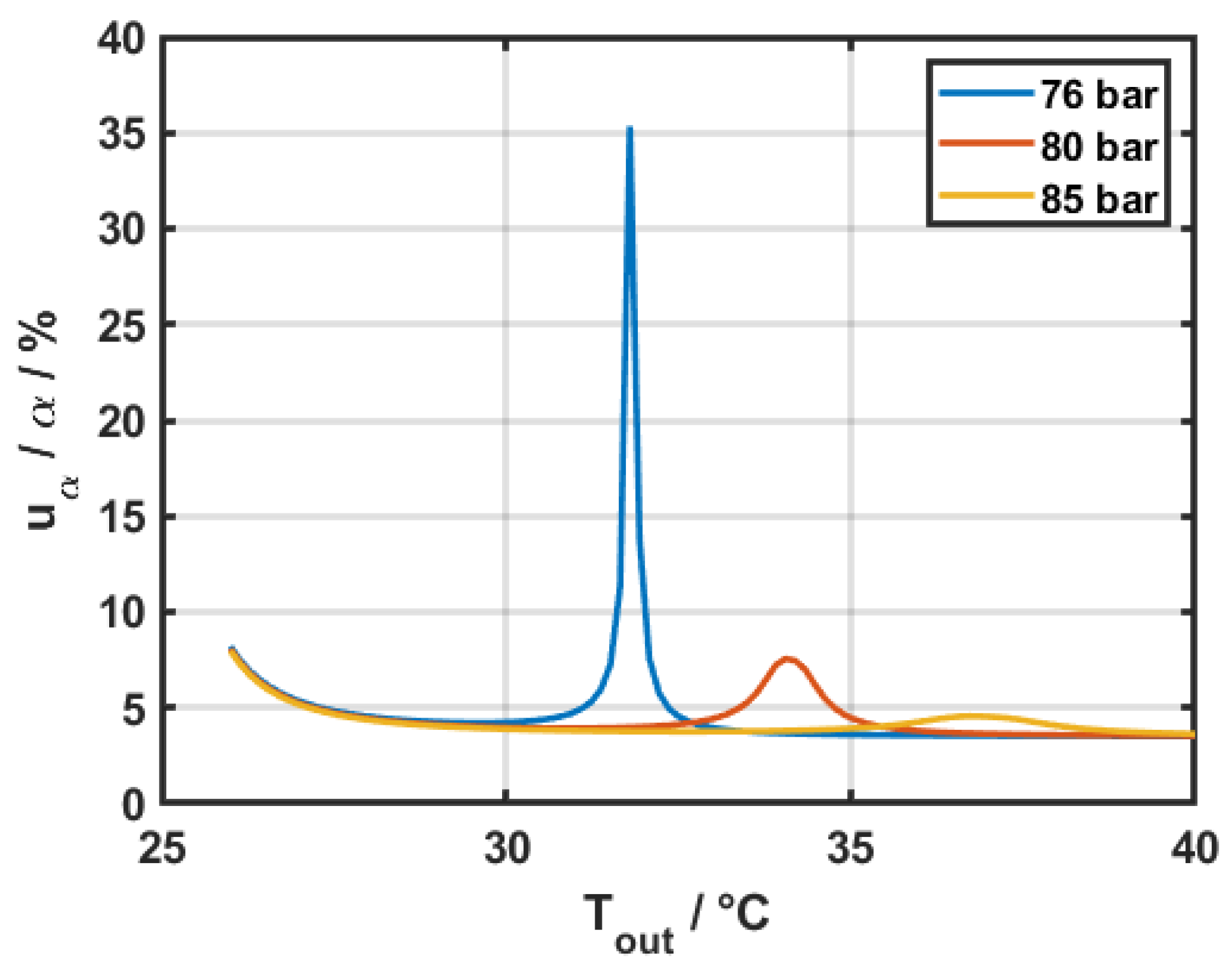
Finally, Figure 8 shows the variation of the relative error in the heat transfer coefficient for fixed inlet conditions at three different operational pressures, while varying the outlet temperature in a mm pipe with a heated length of mm. Pressure drop data was fixed at bar for all three cases and the temperature difference between wall and bulk fluid () was assumed to be 3 K.
9. Validation
Validation of the test rig under conditions where established correlations are applicable is a necessary step before extracting data in the supercritical regime. For this purpose, measurements were carried out at sub-critical liquid conditions, where the thermophysical properties do not change or vary only moderately along the pipe. Under these conditions, both the pressure drop and the heat transfer coefficient can be directly compared with well-established correlations.
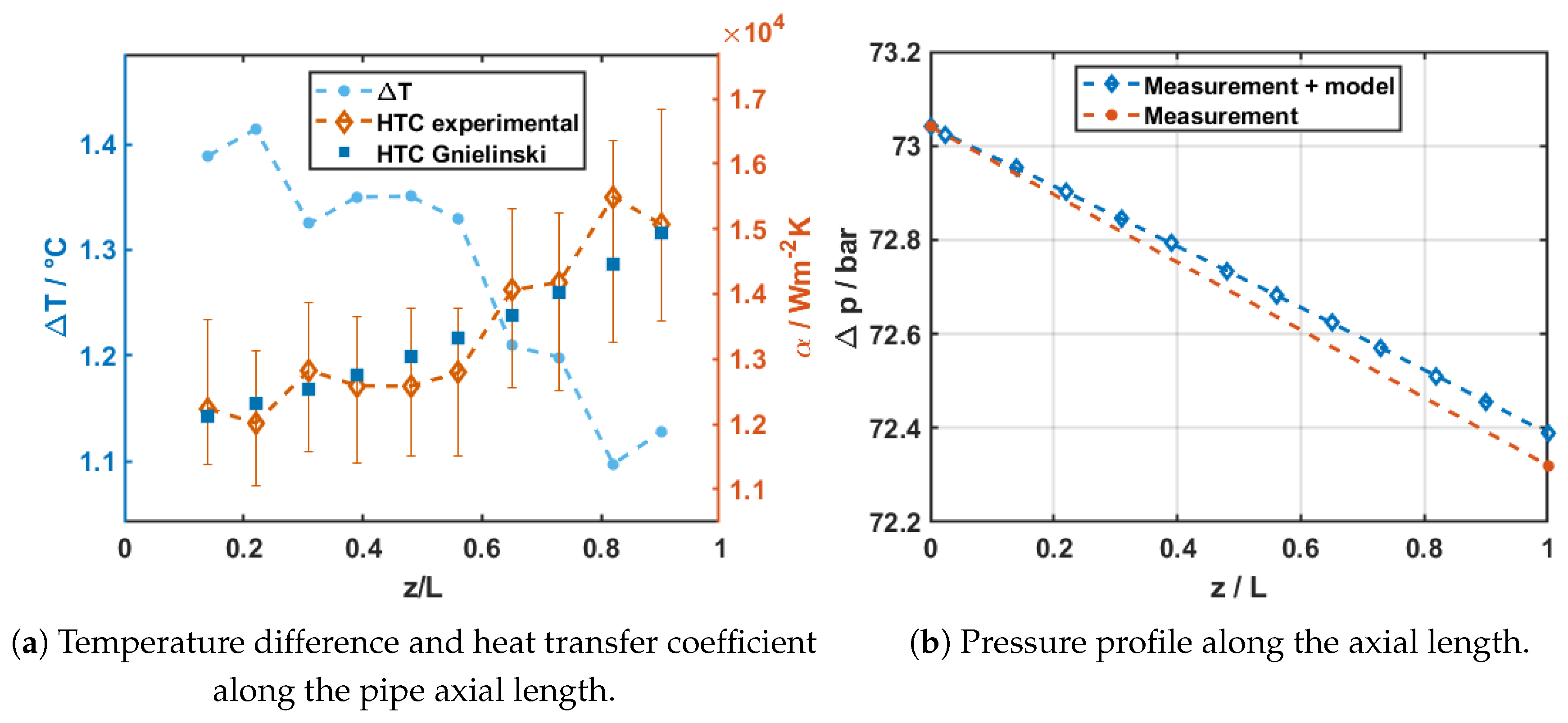
Figure 9 shows the measured wall–to–bulk temperature difference along the heated section, together with the resulting experimental heat transfer coefficient profile. For comparison, heat transfer coefficients were evaluated using the Gnielinski correlation. The data reduction procedure is that specified in Section 7.
Uncertainty bars are included, representing the propagated uncertainty of the heat transfer coefficient as described in Section 8.
Overall, the measured heat transfer coefficients are in very good agreement with the Gnielinski correlation. Additionally, the calculated pressure drops are well captured by the Darcy–Weisbach/McAdams approach, with errors below . This confirms that the test rig is operating reliably and provides confidence in its use for subsequent measurements under supercritical conditions.
In view of the Figure, it is observed that the uncertainty bars become larger at smaller values, which goes in line with the trends deducted in this manuscript.
Figure 9.
Results of the sub-critical subcooled test validation with carbon dioxide at bar, oC, W, g/s, mm, m, m.
Figure 9.
Results of the sub-critical subcooled test validation with carbon dioxide at bar, oC, W, g/s, mm, m, m.
10. Conclusions
A modular test rig to study heat transfer with supercritical carbon dioxide has been developed and validated. All necessary technical information has been included in this manuscript. In addition, the individual calibration of wall and in-fluid temperature sensors has been presented in detail and the importance of accurate temperature measurements for heat transfer coefficient derivation has been demonstrated. To support this, an in-depth calculation of the uncertainty relative to the experimental local heat transfer coefficient has been carried out. This analysis has shown that the temperature uncertainty dominates when the wall–bulk temperature difference is small, while the enthalpy-change term becomes critical near the pseudo-critical region due to its strong sensitivity with respect to temperature and pressure.
The authors therefore emphasize the importance of a detailed, individual and well reported calibration of the sensors involved in precise heat transfer coefficient measurements.
Finally, experiments with sub–critical subcooled liquid flow were carried out to validate the experimental mesurements with respect to analytical calculations. The comparison with known correlations and models has shown good agreement with the theory, showing the robustness of the rig and its acquisition system.
The rig will continue its operation and studies characterizing the heat transfer coefficient and pressure drop at supercritical conditions are soon expected.
Supplementary Materials
The following supporting information can be downloaded at the website of this paper posted on Preprints.org.
| Name | Type | Description |
| charts | Images (.zip) | Miscellaneous images used for the development of the p-h diagram in the front panel |
| config | Configuration files (.zip) | Constants related to the positions of sensors and their calibration constants specific to the current test section installed |
| controls | Control files (.zip) | Structure of certain variables contained in the main LabView code |
| pictures | Pictures (.zip) | Pictures of the test setup |
| src\labview | LabView code (.zip) | Main and subvis of CO2-SASS |
| sco2 | LabView project (.zip) | LabView project file |
Author Contributions
Pedano-Medina, C.: conceptualization, design, procurement, construction, implementation, commissioning, software, data analysis, manuscript. Petagna, P.: supervision, manuscript. Gleissle, S.: supervision.
Funding
This project has received funding from the European Union’s Horizon 2020 Research and Innovation programme under Grant Agreement No 101004761. This work was supported by the Wolfgang Gentner Programme of the German Federal Ministry of Education and Research (BMBF).
Institutional Review Board Statement
Not applicable.
Acknowledgments
The electrical cabinet of this test rig was built by Andrzej Baran (CERN). Further work performed by Jarl Pettersen (CERN). The data acquisition software was designed with the help of Elena Galetti and the BE-CEM-MTA section at CERN.
Conflicts of Interest
The authors declare no conflicts of interest.
Abbreviations
The following symbols and variables are used in this manuscript:
| A | Heat transfer surface area [m2] |
| Specific heat at constant pressure [J kg−1 K−1] | |
| Correction Factor for conduction [-] | |
| Cross-sectional area of flow [m2] | |
| Inner diameter of tube [m] | |
| Outer diameter of tube [m] | |
| f | Darcy friction factor [–] |
| h | Specific enthalpy [J kg−1] |
| L | Total tube length [m] |
| Heated length of tube [m] | |
| Mass flow rate [kg s−1] | |
| Nusselt number [–] | |
| p | Pressure [bar] |
| Inlet pressure [bar] | |
| Outlet pressure [bar] | |
| Prandtl number [–] | |
| q | Heat input [W] |
| Heat flux [W m−2] | |
| Total heat transfer rate [W] | |
| Reynolds number [–] | |
| T | Temperature [K or °C] |
| Bulk fluid temperature [K or °C] | |
| Inlet temperature [K or °C] | |
| Outlet temperature [K or °C] | |
| Wall temperature [K or °C] | |
| Enthalpy difference [J kg−1] | |
| Pressure drop [bar] | |
| Wall–to–bulk temperature difference [K] | |
| Wall temperature difference (outer–inner wall) [K] | |
| u | Standard uncertainty [various units] |
| Relative uncertainty of quantity x [%] | |
| Heat transfer coefficient [W m−2 K−1] | |
| Thermal conductivity [W m−1 K−1] | |
| Dynamic viscosity [Pa s] | |
| Geometrical relationship between outer and inner diameter [-] | |
| Density [kg m−3] | |
| z | Axial coordinate along the tube [m] |
| Dimensionless axial coordinate [–] |
Appendix A. Thermocouple Calibration
Thermocouples measure voltage difference between a hot and a cold junction. This means, when the voltage difference is the output of the DAQ, this corresponds to:
which, by the working principle of a thermocouple, corresponds to:
To calibrate each thermocouple individually from the temperature at the cold junction, must be calculated.
The cold junction temperature is obtained from the thermistor voltage using a voltage divider and the Steinhart–Hart equation:
The ITS-90 defines two equations to obtain temperature from voltage and viceversa:
To convert a measured voltage E (in millivolts) to temperature in degrees Celsius, the inverse polynomial equation is used (valid for ):
The workflow of the calibration procedure is shown in Figure A1. The data from the top is acquired at the same time in the conditions specified above. The rhomboids represent conversions or processes applied to the data. The goal of this process is to:
- Obtain individual equations to describe the thermocouple behaviour in the range of interest.
- Characterize the cold junction error and evaluate its feasibility for wall temperature measurements.
- Calculate the derived uncertainty of the wall temperature measurement.
Figure A1.
Schematic of the thermocouple calibration and correction process. The SPRT reference temperature is converted to voltage using the NIST ITS-90 equation. Each thermocouple reading is compensated for cold junction effects and corrected for individual behavior using a linear calibration.
Figure A1.
Schematic of the thermocouple calibration and correction process. The SPRT reference temperature is converted to voltage using the NIST ITS-90 equation. Each thermocouple reading is compensated for cold junction effects and corrected for individual behavior using a linear calibration.

The leftmost fit will be the individuated thermocouple result using the electronic cold junction and the rightmost will correspond to the result using an ice bath as a reference. The same applies to Figure A2, where it is observed that the systematic behaviour of the thermocouple in question is quite linear for the operating range, however the intercept of the leftmost fit shows that the systematic correction needed to compensate for the uncertainty of the cold junction temperature is 0.0156 mV. Considering that the sensitivity of a type K thermocouple is , this corresponds to a systematic correction of 0.38 oC. This agrees with the maximum accuracy value reported by NI on their NI9214.
Figure A2.
Voltage calibration for one example probe against ITS-90 equivalent reference voltage.
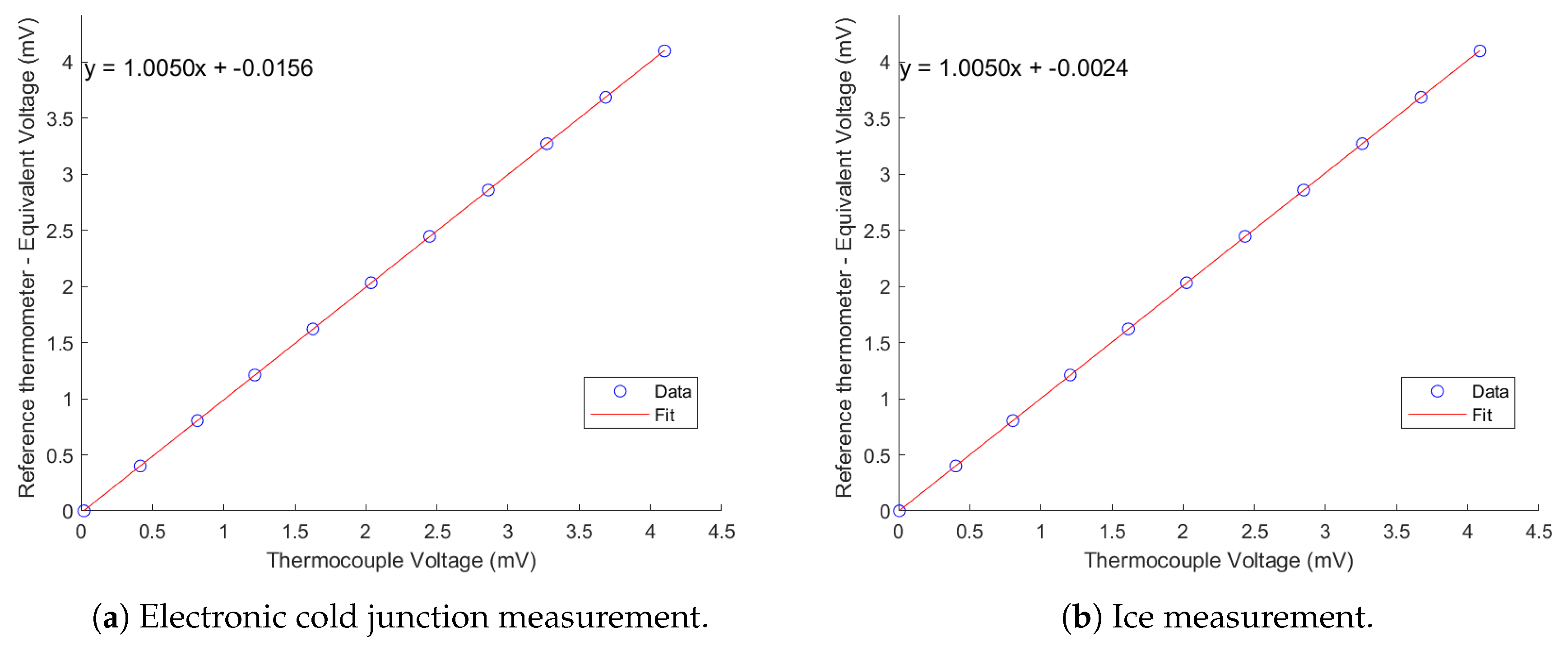
On the other hand, the rightmost fit shows a systematic correction of when the ice bath is used, translating in a systematic temperature drift of oC. This aligns better with the goal of staying below wall temperature error. The maximum error (RMSE) in both cases resulted in 0.021 oC. Physically speaking, the combination of the two offsets results in the cold junction systematic bias, which can be applied to each thermocouple individually to account for the cold junction error.
The two calibration equations obtained for the thermocouple are:
The physical meaning of this subtraction corresponds to the error of the cold junction. This implies that the cold junction measurement introduces a systematic offset of mV. Given the sensitivity of type K thermocouples, this voltage offset translates to a temperature correction of:
This means that, even if the accuracy of the thermocouple calibration is low, the electronic cold junction introduces a significant error in the wall temperature measurement equal to:
Or, equivalently, the corrected temperature could be obtained as:
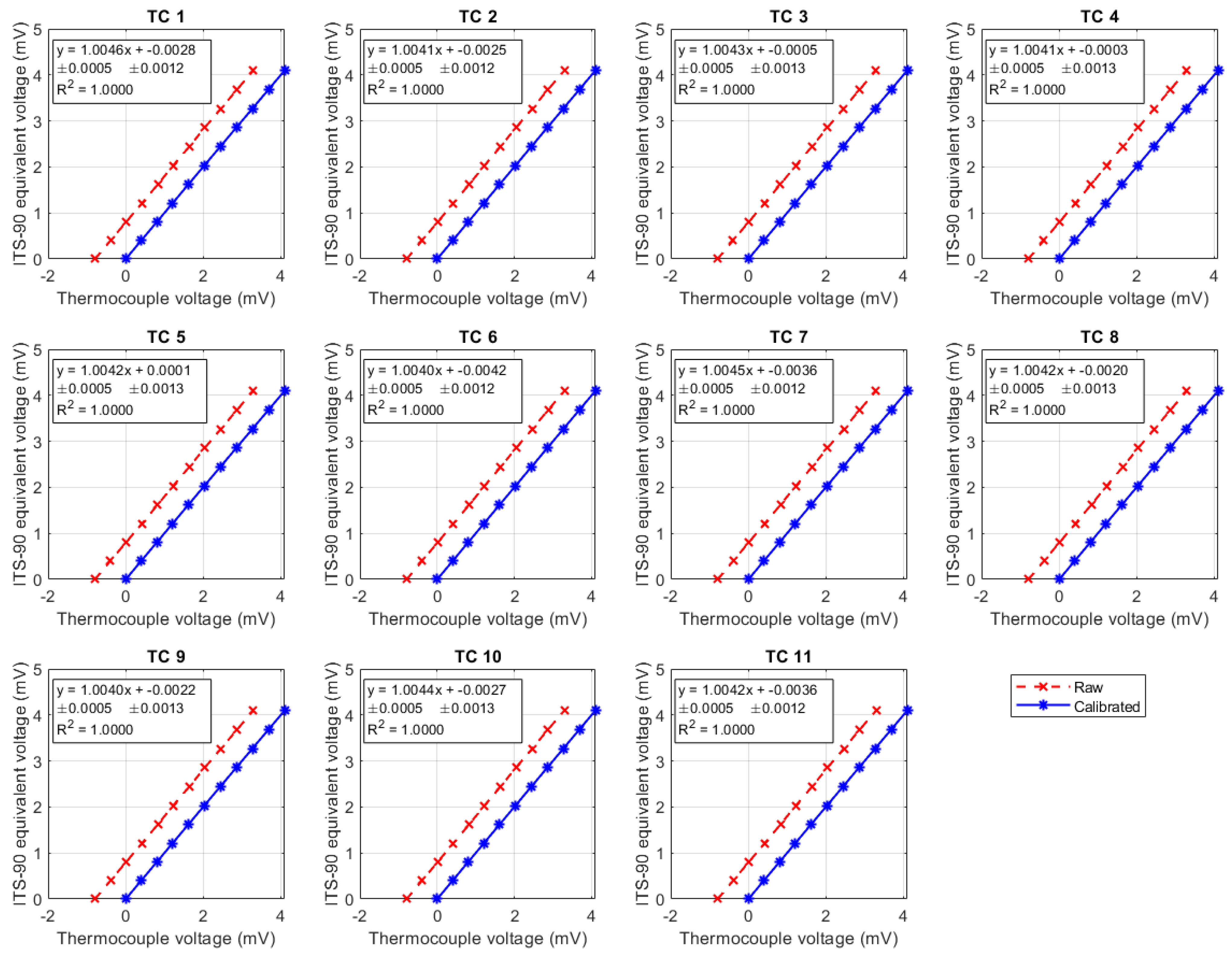
Figure A3.
Calibration fits for wall thermocouples (TC1–TC11). Red: raw measurements; blue: calibrated values. Linear fits with slope and intercept () are shown in each panel, as well as .
Figure A3.
Calibration fits for wall thermocouples (TC1–TC11). Red: raw measurements; blue: calibrated values. Linear fits with slope and intercept () are shown in each panel, as well as .
Appendix B. PT-100
The guidelines of the ITS-90 are based on comparing the resistance ratio of each individual probe to be compared to that of a precise reference thermometer. With the reference thermometer reading (in °C), the reference resistance ratio can be calculated.
The forward coefficients being:
Given the probe’s TPW resistance and the measured resistance R, the ratio and deviation function from the reference can be calculated.
A least-squares fit is performed to obtain the parameter a so that:
Finally, the RMSE can be calculated using:
For which the coefficients are:
Figure A4 shows the least-squares fit as per the ITS-90 for the range 0-oC.
Figure A4.
Calibration of PT100 sensors using the resistance ratio method. Plotted are versus for all nine sensors, with linear fits shown in red. The fitted slopes and RMSE values indicate excellent agreement and reproducibility across sensors.
Figure A4.
Calibration of PT100 sensors using the resistance ratio method. Plotted are versus for all nine sensors, with linear fits shown in red. The fitted slopes and RMSE values indicate excellent agreement and reproducibility across sensors.
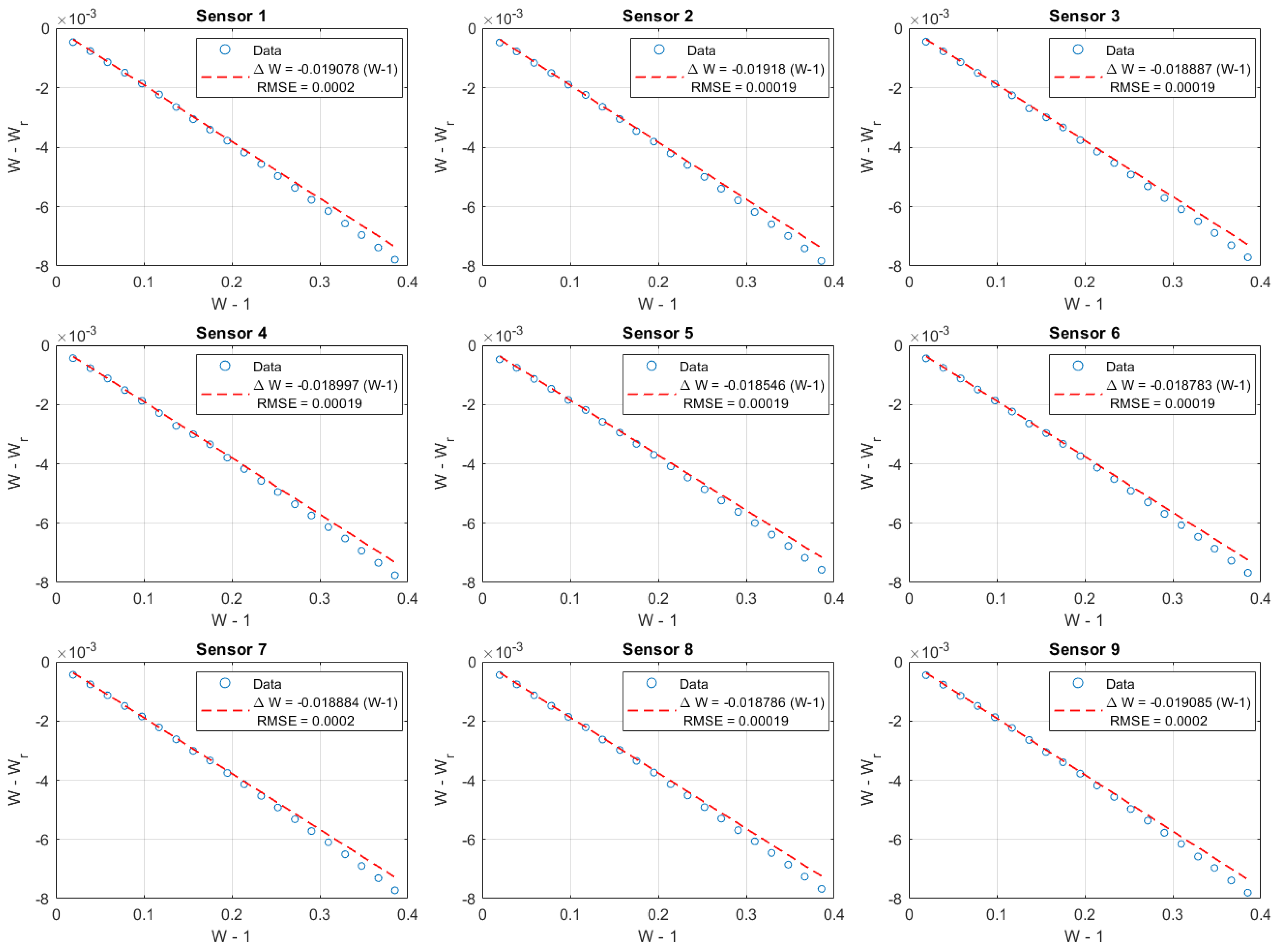
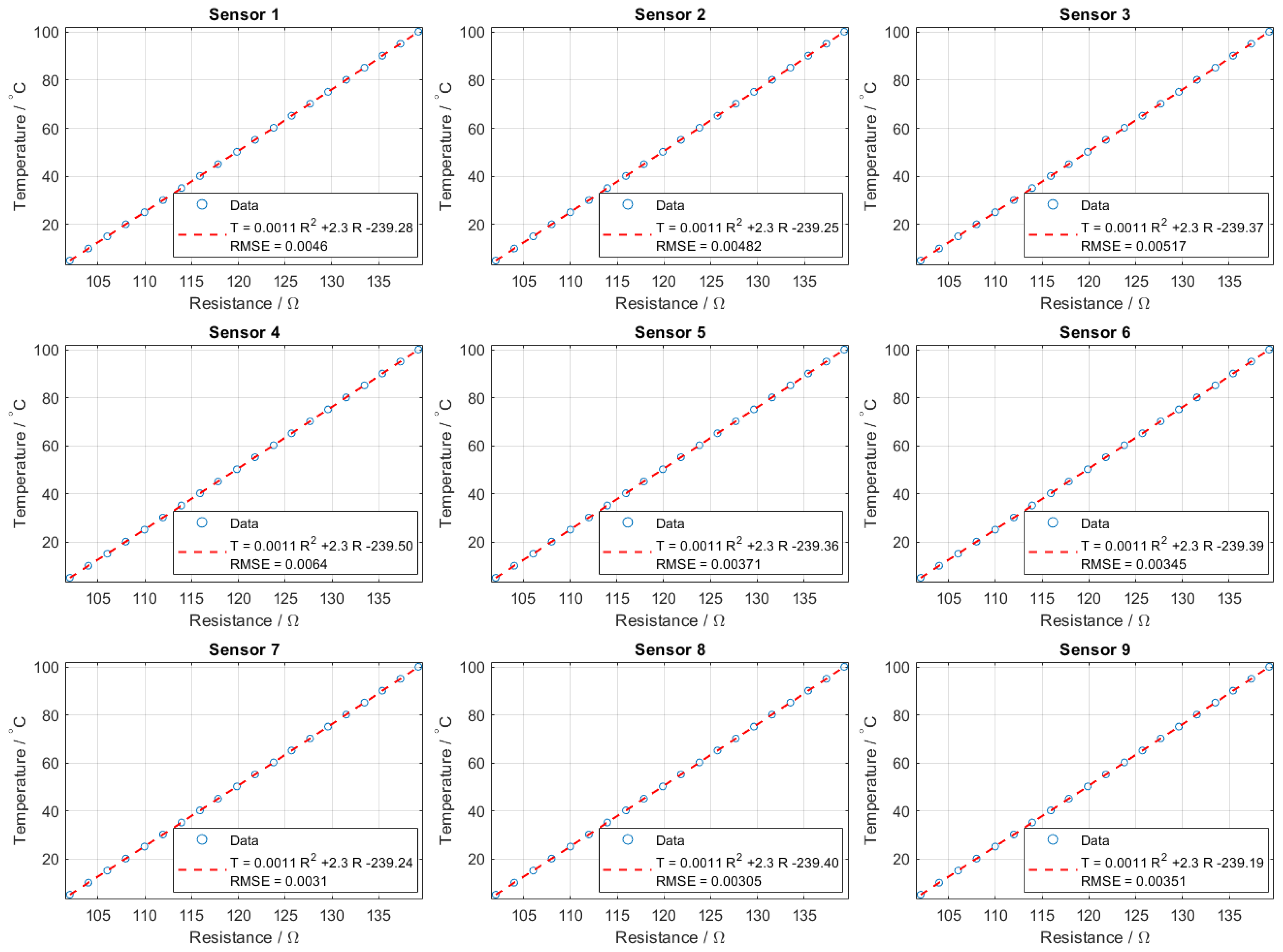
Figure A5.
Operational calibration of PT100 sensors. The plots show temperature as a function of resistance for all nine sensors, with polynomial fits (red dashed) compared against experimental data (blue). RMSE values remain below 0.01 °C, confirming the sensors’ accuracy during operation.
Figure A5.
Operational calibration of PT100 sensors. The plots show temperature as a function of resistance for all nine sensors, with polynomial fits (red dashed) compared against experimental data (blue). RMSE values remain below 0.01 °C, confirming the sensors’ accuracy during operation.
References
- Kwon, J.S.; Son, S.; Heo, J.Y.; Lee, J.I. Compact Heat Exchangers for Supercritical CO2 Power Cycle Application. Energy Conversion and Management 2020, 209, 112666. [CrossRef]
- Mohamed, S. ElGenk. Experimental Evaluation of Supercritical Carbon Dioxide as a Viable Coolant for Electronics Thermal Management. https://www.electronics-cooling.com/2023/12/experimental-evaluation-of-supercritical-carbon-dioxide-as-a-viable-coolant-for-electronics-thermal-management/, accessed on 02/07/2025.
- Fronk, B.M.; Rattner, A.S. High-Flux Thermal Management With Supercritical Fluids. Journal of Heat Transfer 2016, 138, 124501. [CrossRef]
- Guo, P.; Liu, S.; Yan, J.; Wang, J.; Zhang, Q. Experimental Study on Heat Transfer of Supercritical CO2 Flowing in a Mini Tube under Heating Conditions. International Journal of Heat and Mass Transfer 2020, 153, 119623. [CrossRef]
- Lei, X.; Peng, R.; Guo, Z.; Li, H.; Ali, K.; Zhou, X. Experimental Comparison of the Heat Transfer of Carbon Dioxide under Subcritical and Supercritical Pressures. International Journal of Heat and Mass Transfer 2020, 152, 119562. [CrossRef]
- Wang, X.; Yang, L.; Xu, B.; Chen, Z. Experimental Study on Heat Transfer and Flow Characteristics of Supercritical CO2: In-depth Analysis of Three Heat Transfer Coefficients. International Journal of Heat and Mass Transfer 2025, 241, 126748. [CrossRef]
- Liao, S.; Zhao, T. An Experimental Investigation of Convection Heat Transfer to Supercritical Carbon Dioxide in Miniature Tubes. International Journal of Heat and Mass Transfer 2002, 45, 5025–5034. [CrossRef]
- Wang, L.; Pan, Y.C.; Der Lee, J.; Wang, Y.; Fu, B.R.; Pan, C. Experimental Investigation in the Local Heat Transfer of Supercritical Carbon Dioxide in the Uniformly Heated Horizontal Miniature Tubes. International Journal of Heat and Mass Transfer 2020, 159, 120136. [CrossRef]
- Huber, M.; Harvey, A.; Lemmon, E.; Hardin, G.; Bell, I.; McLinden, M. NIST Reference Fluid Thermodynamic and Transport Properties Database (REFPROP) Version 9.1 - SRD 23, 2018. [CrossRef]
- Cabeza, L.F.; de Gracia, A.; Fernández, A.I.; Farid, M.M. Supercritical CO2 as Heat Transfer Fluid: A Review. Applied Thermal Engineering 2017, 125, 799–810. [CrossRef]
- Ferrand, T.; Oettig, J.; Schäfer, L.; Gschnaidtner, T.; Naja, M.O.; Wieland, C.; Spliethoff, H. A Limitation to Determine Heat Transfer of Water at Supercritical Pressure: The Repeatability Issue. Applied Thermal Engineering 2023, 219, 119357. [CrossRef]
- National Institute of Standards and Technology. Ice Point Calibration, 2014.
- J. Buongiorno. Methodologies to Select Friction Factor and Convective Heat Transfer Correlations for Single-Phase Fluids. https://tinyurl.com/shortened-link-to-mit-edu, 2014.
- Wang, Z.; Sun, B.; Wang, J.; Hou, L. Experimental Study on the Friction Coefficient of Supercritical Carbon Dioxide in Pipes. International Journal of Greenhouse Gas Control 2014, 25, 151–161. [CrossRef]
| 1 | The pseudo–critical point refers to a physical condition, in pressure and temperature, at which the heat capacity of a fluid above the critical point experiences a maxima. |
| 2 | Whenever space allows, RTDs would be preferred for simpler and more accurate temperature measurements. NTCs could also be an option, although unfortunately not yet commonly used in the field |
Figure 1.
Thermophysical properties of CO2 as a function of temperature (20 to 50oC) at selected pressures (70, 75, 80, 85, 90 bar). Shown are: density (kg m−3), heat capacity at constant pressure (, kJ kg−1 K−1), viscosity (, µPa s), and thermal conductivity (k, mW m−1 K−1). Property values were obtained from REFPROP [9].
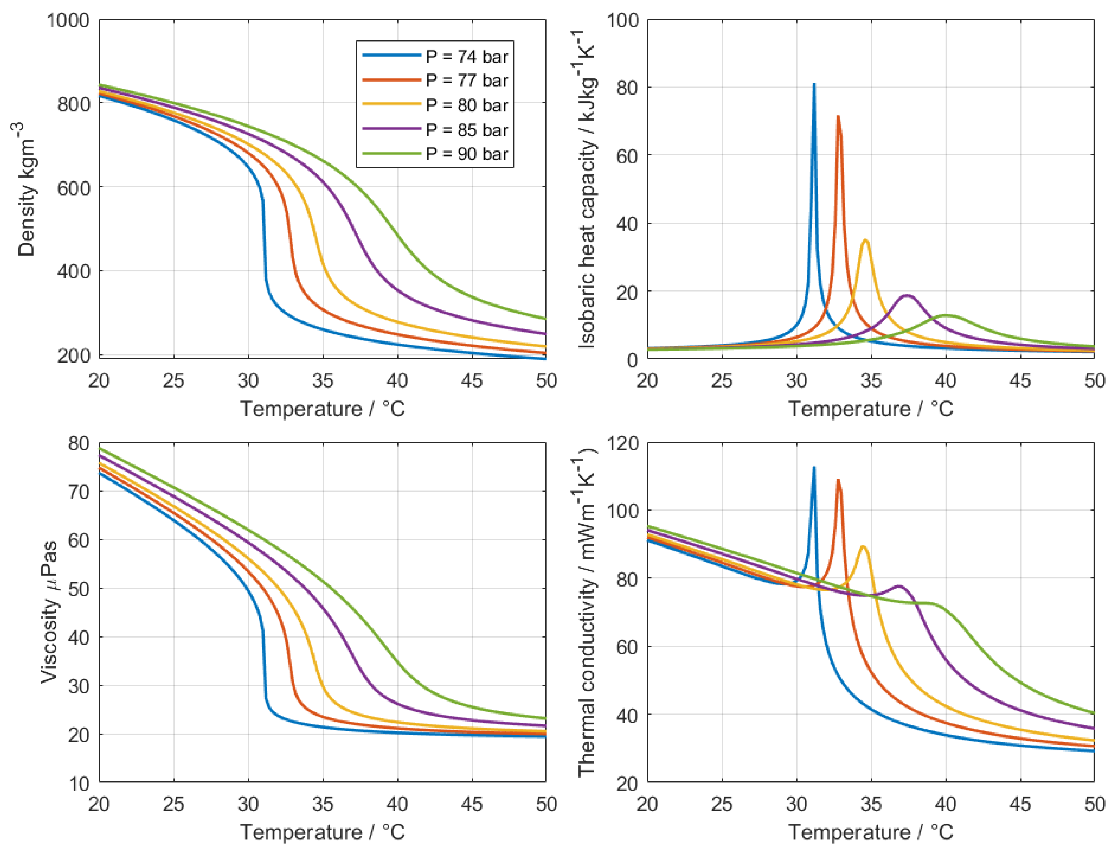
Figure 4.
Schematic representation of the NI modules in the test rig and their corresponding signal types.
Figure 4.
Schematic representation of the NI modules in the test rig and their corresponding signal types.
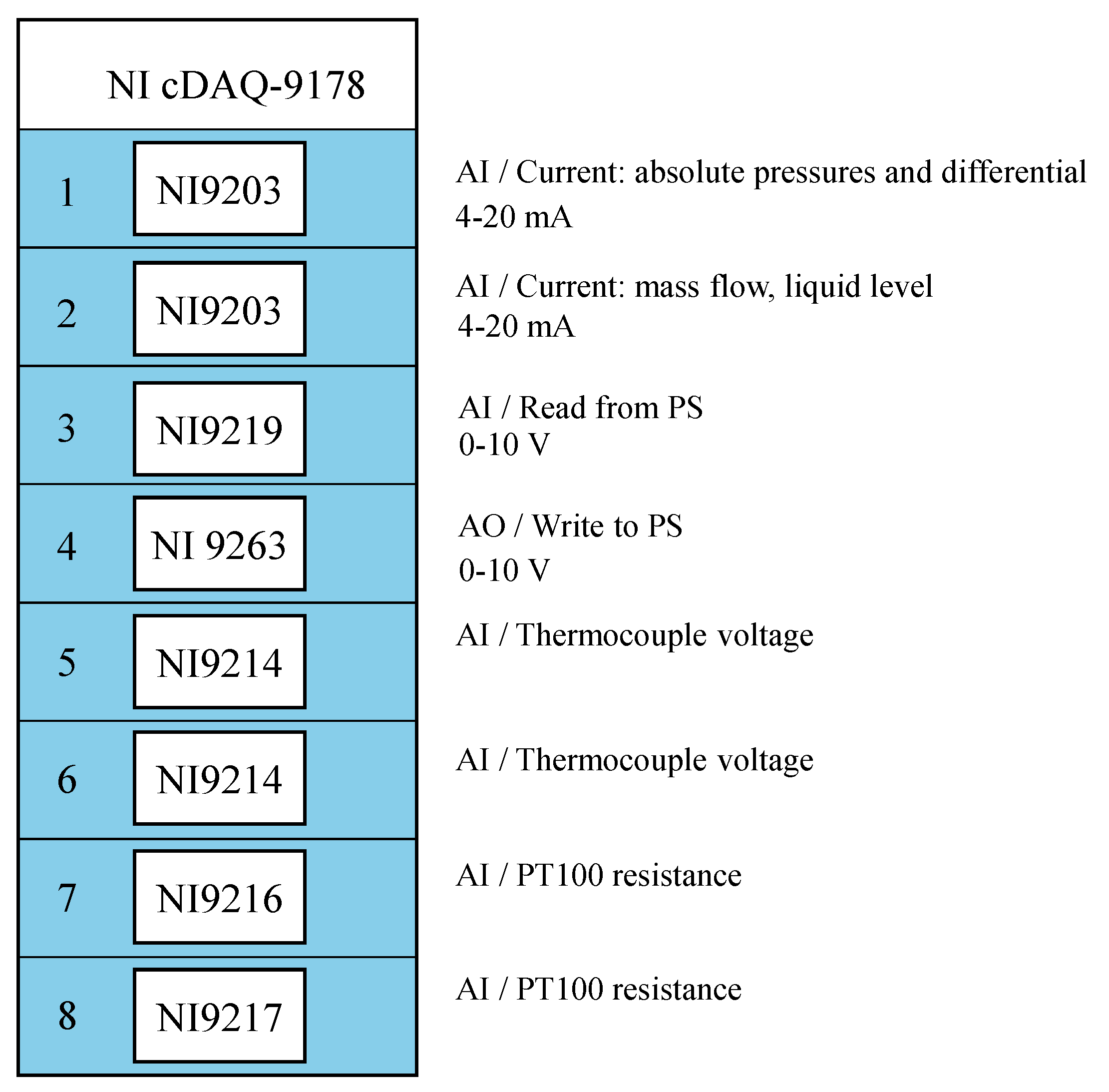
Figure 6.
Relative error in the heat transfer coefficient as a function of the true wall–bulk temperature difference , assuming a fixed measurement uncertainty of C. (a) Small temperature difference range ( (b) Zoom for C.
Figure 6.
Relative error in the heat transfer coefficient as a function of the true wall–bulk temperature difference , assuming a fixed measurement uncertainty of C. (a) Small temperature difference range ( (b) Zoom for C.
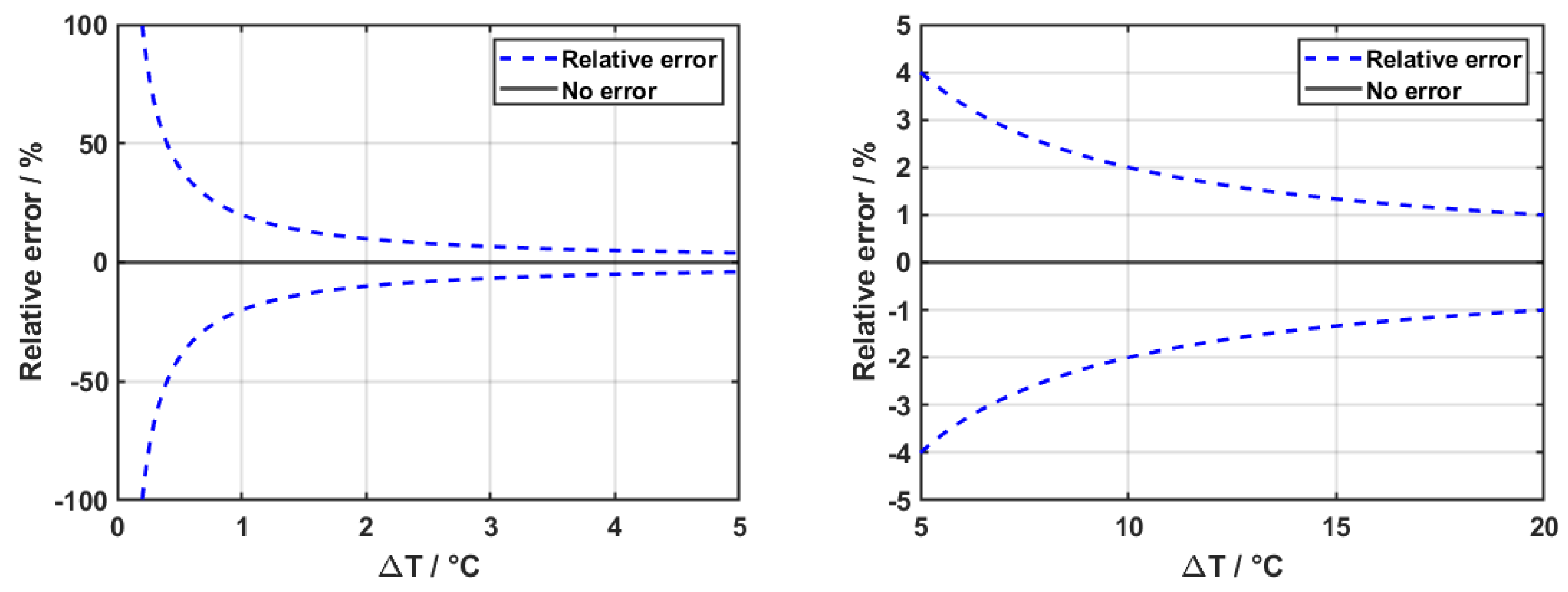
Figure 7.
Thermodynamic property evaluation of in the range 74–90 bar.
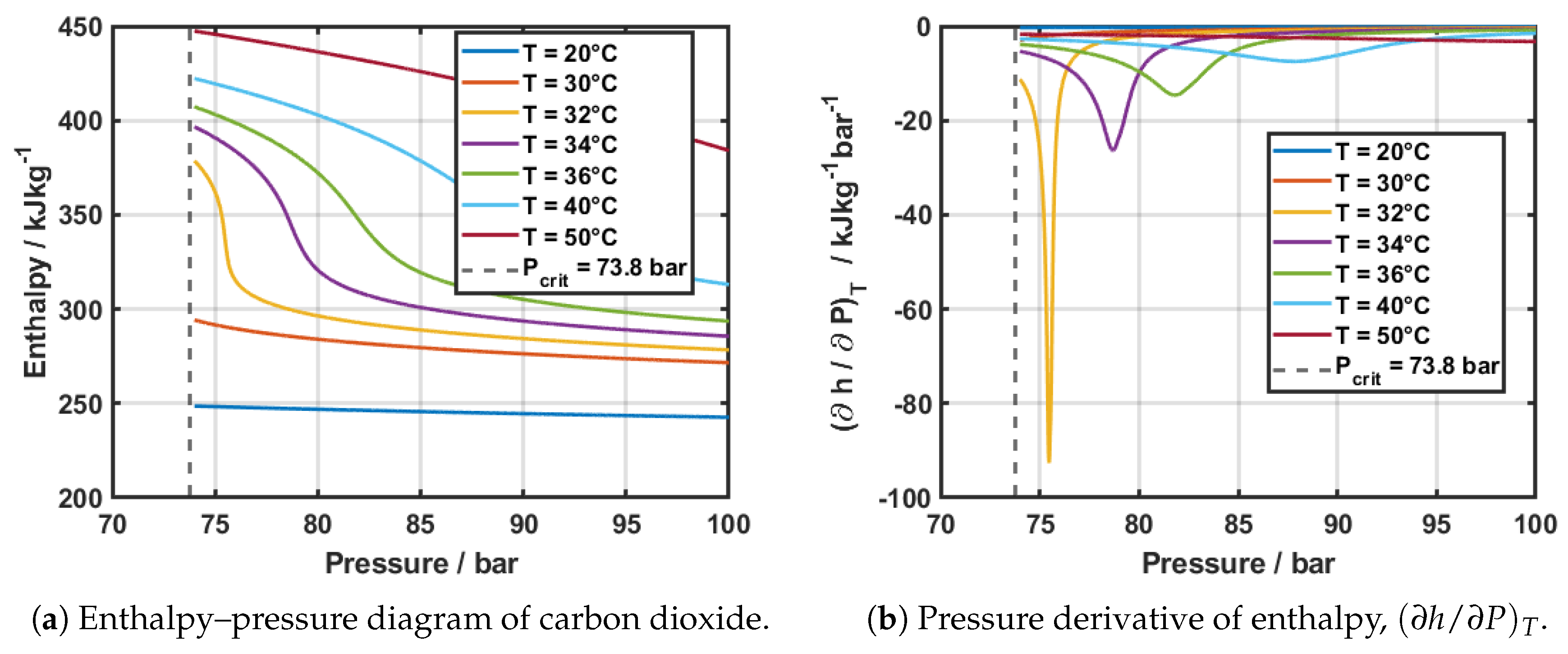
Figure 8.
Total uncertainty of the heat transfer coefficient at fixed inlet conditions: oC, bar; assuming a pressure drop of bar and K. Individual uncertainties of the process parameters are those calculated in Section 6.
Figure 8.
Total uncertainty of the heat transfer coefficient at fixed inlet conditions: oC, bar; assuming a pressure drop of bar and K. Individual uncertainties of the process parameters are those calculated in Section 6.
Disclaimer/Publisher’s Note: The statements, opinions and data contained in all publications are solely those of the individual author(s) and contributor(s) and not of MDPI and/or the editor(s). MDPI and/or the editor(s) disclaim responsibility for any injury to people or property resulting from any ideas, methods, instructions or products referred to in the content. |
© 2025 by the authors. Licensee MDPI, Basel, Switzerland. This article is an open access article distributed under the terms and conditions of the Creative Commons Attribution (CC BY) license (http://creativecommons.org/licenses/by/4.0/).
Copyright: This open access article is published under a Creative Commons CC BY 4.0 license, which permit the free download, distribution, and reuse, provided that the author and preprint are cited in any reuse.


