Improvement of Accuracy and Computational Cost in Analysing Wire Antennas and Scatterers Using CMA

Tuan Phuong Dang; Talgat Rashitovich Gazizov; Minh Tuong Nguyen

doi:10.20944/preprints202510.1863.v1

Submitted:

23 October 2025

Posted:

24 October 2025

You are already at the latest version

Abstract

Problem statement. Antennas and scatterers play a critical role in telecommunications technologies. Accurate analysis is essential for optimizing designs, reducing costs, and predicting real-world behavior. Characteristic mode analysis is a widely used method for studying these interactions, offering insights into how the structural shape and parameters affect radiation and scattering characteristics. Traditional characteristic mode analysis often relies on modal significance to identify significance modes; however, this approach does not fully consider the properties of the eigencurrent and the excitation source, which can lead to potential inaccuracies in determining significant modes.Aim. Develop an algorithm to identify the most significant modes for analysing the characteristics of antenna and scatterers when using characteristic mode analysis and presents the verification of the analysis results of the corner reflector structure using characteristic mode analysis and the effectiveness of the algorithm used.Results. Two algorithms have been developed to improve both the accuracy and the computational efficiency in analyzing wire antenna and scatterers using characteristic mode analysis. The first algorithm considers the properties of the eigencurrent and the excitation source to determine the significant modes. The second algorithm reduces the computational cost while maintaining high precision. The accuracy and effectiveness of these two algorithms have been demonstrated in the analysis of dipole antenna and a variety of corner reflector as scatterers.Practical significance. The proposed algorithms can be used to identify significant modes in the analysis of wire antenna and scatterer structures, thereby making the optimization of these structures using characteristic mode analysis more accurate.

Keywords:

antenna

;

characteristic mode analysis

;

current distribution

;

method of moments

;

scatterer

Subject:

Engineering - Electrical and Electronic Engineering

Introduction

Antennas and scatterers play an important role in many fields of modern life, from telecommunications to radar technology [1,2]. The interaction of electromagnetic waves with antennas or scatterers can significantly affect the performance of communication systems. Therefore, accurate simulation and analysis of the characteristics of antennas and scatterers is necessary to optimize the design and performance of these systems.

Modeling antennas and scatterers not only improves their designs but also aids in predicting the behavior of electromagnetic waves in practical situations. Without simulation, it is difficult to understand how electromagnetic waves interact with these elements, which can lead to suboptimal designs or unsatisfactory performance. In addition, simulations allow researchers and engineers to test different scenarios without having to build actual models, thus saving time and money [3].

There are various methods used to analyze antennas and scatterers, one of which is characteristic mode analysis (CMA). CMA was developed based on MoM [4] and focuses on analysing the modes of the structure. Each CMA mode corresponds to a specific way of energy transfer occurring in the structure, so CMA-based structure analysis helps to better understand how the shape and parameters of the structure affect its ability to radiate or scatter. Therefore, using CMA helps engineers to adjust the shape and structure of antennas to achieve good performance [3]. In addition, CMA can also be applied to structures with complex shapes and does not require the inversion of the impedance matrix like the conventional MoM [4], which is another notable advantage of it.

In the CMA-based analysis of antennas and scatterers, determining which modes have the large influence on the surface current and the far field during radiation and scattering is essential to obtain correct analysis results. Previously, researchers often relied on and pointed out that it is enough to use only a few modes with the largest modal significance (MS) values to analyze surface current [5]. However, our simulations of complex structures demonstrated that considering only MS is not enough; it is also crucial to consider the characteristics of eigencurrents and excitation vector. In addition, the creation of sparse antennas and scatterers using CMA is a new development direction worth considering. As such, determining which modes influence the analysis results (surface current and far field distribution) is clearly necessary. CMA has been widely applied in the optimization and analysis of various antenna types. On the other hand, it is also necessary to verify the analysis results of complex scatterer structures, for example, corner reflectors (CRs), using CMA to demonstrate the algorithm accuracy for such structures.

The aim of paper: develop an algorithm to identify the most significant modes for analysing the characteristics of antenna and scatterers when using CMA and presents the verification of the analysis results of the CR structure using CMA and the effectiveness of the algorithm used.

Algorithm for Determining Significant Modes

Among various electromagnetic simulation methods, MoM has attracted significant attention. After applying MoM to an antenna or scatterer, the impedance matrix Z (N×N) is obtained with N being the number of basis pulse functions (also equal to the number of segments) [6]. After applying CMA as [7], the eigenvalue λ_n, and eigenvector I_n (or characteristic current) (N×1) (where n is the index of the corresponding mode) are found for the structure based on the formula

where R and X are the real and imaginary parts of matrix Z, respectively. The surface current (i) then can be determined as following [4]:

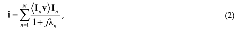
where v is the excitation vector. From (2), it is seen that i is inversely proportional to λ_n. A value presented in [8,9] to characterize the influence of the n-th mode on i is called modal significance (MS_n), and is calculated as

Equation (2) illustrates that MS_n depends only on λ_n. While λ_n has a value in the range (–∞; +∞), MS_n has a value in the range 0–1. From (2) and (3), it can be seen that if the considered modes have the same I_n value and are excited similarly, the larger the value of MS_n, the larger the obtained i and conversely, the MS_n closer to 0, the lower the contribution of that mode to i. A threshold based on the half-power modal significance is set in [8] to determine the n-th mode as significant or non-significant.

However, from (2) and some experiences through the modeling process, we found that in addition to MS_n, the characteristics of the source (amplitude, excitation position in the case of antennas; amplitude, direction, polarization of incident wave in the case of scatterers) and the I_n value of different modes also have a significant influence on the i. Therefore, we can suppose that to determine significant modes, it is not enough to consider only MS_n, as in previous studies, but it is also necessary to consider both modal excitation (scalar product <I_n, v>) and the value of I_n. Thus, it is necessary to consider the product of modal excitation, I_n and MS_n

p_n=<I_n, v>I_nMS_n. (4)

In the case of antennas, according to [10], v has the form [0, ..., V_i, ..., 0], where i is the index of the i-th segment where an antenna is excited. At this time, modal excitation <I_n, v> is determined by the product of i-th value in the I_n vector with V_i=1 V (the amplitude of the excitation voltage).

The resulting p_n is a vector for the n-th mode. If the sum of the absolute values of the entries in p_n is larger, the n-th mode has a greater influence on the i and vice versa. Comparisons between p_n are made by averaging their magnitude elements (p_n^mean). The p_n with a larger average value is considered to have more influence on i.

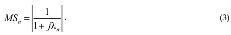
Figure 1 shows the algorithm for identifying significant modes in this study.

Dipole Antennas Analysis

When using CMA at a given frequency, the modes are usually arranged based on the increasing value of |λ_n| (decreasing value of MS_n) [4]. Therefore, according to the theory used in previous studies, the modes with smaller indexes will be considered as significant modes.

First, we determined the mode that affects the surface current most for dipole antennas D1 with the length l=2 m and the radius a=4.2 mm operating at frequency 300 MHz. The dipole is divided into 75 segments and is excited at the midpoint (38-th segment).

After using CMA, the MS_n values of modes 1–9 are respectively MS₁=0.79, MS₂=0.39, MS₃=0.38, MS₄=0.37, MS₅=0.05, MS₆=0.03, MS₇=0.00015, MS₈=6.2e-6, and MS₉=2.4e-7. Figure 2a illustrates the dependences of I_1–9 on x along the D1 length. The dependences of p_1–9 on x along the length of D1 are shown in Figure 2b. From Figure 2a, it can be seen that modes 1, 2, 4, 6, and 8 have I_n=0 value at the source position (midpoint D1), so p_n of these modes will all be 0. In addition, it can be seen that I₃ is smaller than I_{5, 7, 9} but MS₃ is much higher than MS_{5, 7, 9}, so p₃ obtained is the largest (Figure 2b). Meanwhile, mode 5 has MS₅ about 7.5 times smaller than MS₃ but the maximum of I₅ (as well as I₅ at the source position) is about double, so p₅^max is about 1/2 of p₃^max. Furthermore, Figure 2a illustrates that I_{7, 9} are much higher than I₃, ₅; however, MS_{7, 9} are very small (compared to MS_{3, 5}), so p_{7, 9} is also quite small compared to p_{3, 5}, but they still affect i (Figure 2b). These conclusions imply that when calculating i for D1 using CMA, it is necessary to use modes 3, 5, 7, and 9 to achieve accurate results.

To verify the results of the mode prediction for D1, |I| and ϕ_I obtained using MoM were compared with those obtained using CMA with different mode types (modes based on p_n were 3, 5, 7, and 9; and modes based on MS_n were 1, 2, 3, and 4) (Figure 2c,d). |I| and ϕ_I obtained using CMA with modes 3, 5, 7, and 9 demonstrate good agreement with those obtained using MoM. However, |I| and ϕ_I for modes 1–4 have completely different shapes compared to those obtained using MoM and CMA with modes 3, 5, 7, and 9. Specifically, |I| when using CMA with modes 1–4 has only 3 large peaks, while |I| when using MoM and CMA with modes 3, 5, 7, and 9 has 4 peaks.

This might have happened because using CMA with modes 1–4, only mode 3 actually has a large influence on I (I₃ is similar to the obtained |I|) without considering the contributions of other significant modes (modes 5, 7, and 9). The abrupt change of |I| at the source location occurred when using MoM but not when using CMA. This currently has no satisfactory explanation and will be considered in future work.

Next, we compared the RP obtained using MoM with that obtained using CMA with different mode types (Figure 2e). Due to the large difference between i obtained for different mode types, the RP for modes 1–4 was also different from that for modes 3, 5, 7, and 9 (as well as with MoM).

Scatterers

Dipole scatterer. Next, we determined the modes that have a strong influence on the scattering ability of the dipole scatterer structure. In this case, we considered dipole scatterers D2, that have the dimensions l=1.5 m, a=4.7 mm, is divided into 51 segments. The scatterer excitation source is a plane wave with θ-polarization, an amplitude of 1 V/m, and perpendicular to the plane containing the dipole. In this case, all segments on structures D2 have the same voltage (because they have the same length). Therefore, the excitation vector has the form [v, v, ..., v] with the size of 1*N. The modal excitation of each mode is equal to the sum of the real values of all elements in I_n. Therefore, in general case, it can be concluded that the larger the MS_n and I_n values of a mode, the more that mode contributes to i and vice versa.

The I_n and p_1–3 values for D2 depending on x are shown in Figure 3a,b. For the D2 dipole, after using CMA, the MS values obtained for the first 3 modes are respectively MS₁=0.78, MS₂=0.39, MS₃=0.39. Observing Figure 3a, one can see that I₂ is symmetric about the zero axis, p₂ is zero, i.e. it does not affect the surface current of D2 in the considered case. I₁ and I₃ are both asymmetric about the zero axis, so p_{1, 3} is different from zero and has a large influence on the current (where MS₁=0.78 is larger than MS₃=0.39, while I_{1, 3}^max are almost the same, so p₁ is also larger than p₃). From the above conclusions, it can be predicted that using mode 1 and mode 3 is sufficient to simulate i.

The current obtained using MoM was then compared with the current obtained using CMA with different modes (modes based on p_n were 1 and 3, and modes based on MS_n were 1 and 2) (Figure 3c,d). It is clearly seen that using CMA with modes 1 and 3 produced i results that match very well with MoM results, while using CMA with 1 and 2 produced i results that have a different shape than MoM. This can be explained by the fact that when using CMA with only modes 1 and 2, the shape of obtained |I| will be identical to I₁ (mode 2 has no effect on i), while I₃ also has an effect on i. When only modes 1, 2 are used without mode 3, the |I| in the segments in the middle of the dipole is higher, while the two sides are smaller than it is when using CMA with modes 1, 3. It is because I₁ and I₃ in the middle of the dipole (x=18–34) have opposite signs and the two sides (x=1–18 and x=34–51) have the same sign. In addition, ϕ_I of the dipole using CMA with modes 1 and 2 is clearly different from that using CMA with modes 1 and 3 and MoM.

Next, we calculated the scattered field by the dipole in the ϕ=0° plane using MoM and CMA with different modes (Figure 3e). Logically, the currents obtained using MoM and CMA with modes 1 and 3 match well, so the scattering field obtained by them also matches well. Meanwhile, the scattering field by the dipole when using CMA with modes 1 and 2 is significantly different from other methods even at the main lobe (10 V/m at θ=90° for MoM, 6.9 V/m at θ=45° for CMA with modes 1 and 2) and the side lobe (5.9 V/m at θ=45° for MoM, 5 V/m at θ=90° for CMA with modes 1 and 2).

Plate scatterer. Since the excitation mode of the scatterer is considered to be more complex than that of the antennas, we continued by considering the influence of modes when using CMA for more complex scatterers (SP plate). SP is located in the xOz plane, has a height H=1.6 m, a length L=1.2 m and is excited by a θ-polarization plane wave with an amplitude of 1 V/m. When simulating the plate using the wire grid (WG) model, it is divided into rectangular cells with 15 cells along the height and 10 cells along the length (a total of 325 segments) and a wire radius of 17 mm. Each WG cell wire is represented by one segment.

The case considered was the incident wave with a frequency of 300 MHz directed orthogonally to the plate surface. Using the CMA analysis, we considered 12 modes to perform the plate simulation. Based on the p_n analysis, the modes that are likely to have a large impact on i were 3, 5, 9, 13, 16, 21, 30, 32, 34, 40, 56, and 57, while the commonly used modes based on the highest MS_n values are modes 1–12. The |I| and ϕ_I values obtained using MoM were compared with the current using CMA with different modes (Figure 4a,b).

It was found that using CMA with p-based modes produced |I| and ϕ_I that match very well with those obtained using MoM. Meanwhile, using CMA with modes 1–12 results in a large deviation from i (|I| is smaller on the vertical segments at the edge of the plate and ϕ_I deviates significantly from MoM). The small current obtained at x=1–160 (horizontal wires) can be explained by the fact that the horizontal segments were not affected by θ-polarization. Meanwhile, the |I| value obtained using CMA with modes 1–12 on the horizontal segments was obtained with quite high magnitude, which is unreasonable. The currents obtained at segments x=161–175 and x=311–325 (i.e. vertical segments located at the two edges of the plate) were the highest, which is consistent with the scattering properties of the flat plate.

Next, the scattered field obtained using different methods was analyzed (Figure 4c,d). It was found that in both ϕ=90° and θ=90° planes, the CMA based on p_n produced a scattered field that is in good agreement with the MoM. However, the CMA with modes 1–12 is more deviated (deviation for maximum E is about 10 V/m, and for side lobe in θ=90° plane it is about 2.8 V/m). The main lobe level when using the CMA with modes 1–12 is lower than that when using MoM because the |I| obtained is significantly lower on the vertical segments located on the edges of the plate. The main lobe in the θ=90° plane is wider than in the ϕ=90° plane because the length is smaller than the height.

Reduction of Computational Resources When Analyzing Scatterers Using CMA

Sections III and IV presented the revealing of the most significant modes when analyzing simple antennas and scatterers using CMA. However, the determination of the number of modes needed to analyze the structures was not considered. At the same time, it was found that calculating pn of all modes and analyzing the influence of each mode in complex structures (made up of many segments) can make the analysis time very large. Therefore, reducing the computational cost when analyzing complex structures using CMA is really necessary.

The algorithm for reducing computational resources when analyzing scatterers using CMA is shown in Figure 5. The reduction in computational time is based on selecting the most significant modes by comparing the p_n^mean values with T_p×p_n^mean_max (where T_p is a chosen threshold value). In this paper, we use T_p=0.1 to obtain accurate results while reducing the time required for analysis. Note that choosing a high T_p may result in inaccurate analysis results, while a low T_p will increase computational time.

However, considering significant modes using only T_p helps to reduce analysis time. Specifically, to analyze complex structures that require many segments (for example, tens of thousands), it is necessary to store all I_n and MS_n to determine all p_n and then compare them with T_p×p_n^mean_max which will require a lot of memory. Therefore, in this work, we use the thresholds T_I and T_MS to initially remove modes with small I_n and MS_n. This will help to store I_n, MS_n, and p_n which requires less memory if compared with the case of considering all modes. In this work, we use T_I=T_MS=0.01.

To verify the results of CMA based on our algorithm obtained for scatterers, different structures were considered: plate scatterer S1 from [11], dihedral CR (DCR) S2 from [11], S3 from [12], S4 from [13], and triagular trihedral CR (TTCR) S5 from [14]. The backscattering cross section (BSCS) results obtained using CMA were compared with those obtained using measurement and other numerical methods such as: MoM with piecewise-sinusoidal basis function (PWS) [11], Physical Theory of Diffraction (PTD) [12], MoM in FEKO, Ray Launching-Geometrical Optics (RL-GO) [13], shooting and bouncing ray (SBR), multilevel fast multipole method (MLFMM) [14], and MoM based on WG with pulse basis function (PBF).

The equivalent WG DCR and TTCR structures are illustrated in Figure 6. DCR structure is formed by two rectangular plates (A and B) whose intersection coincides with the Oz axis and the angle between them is 2γ (for S2, it is 130°, and for S3 and S4, it is 90°). Both plates are characterized by the height (H) and the length (L).

The perfect conducting TTCR is made of 3 isosceles right triangles, with the height H and the length of the base leg L. The surfaces of the TTCR lie in the xOz, yOz, xOy planes, and they are orthogonal to each other. The origin of the coordinate system coincides with the intersection point between their surfaces.

In this publication, solid scatterers were first approximated by WG, then these WGs were analyzed using CMA with the approach mentioned in Figure 5 and compared with the scattering characteristics of the solid structure taken from the published papers [11,12,13,14]. When modeling the considered scatterers by WG, their plates were divided into cells of equal size and edge length of Δ (Figure 6) (each WG cell edge was considered to be as one wire represented by one segment with a length Δ). The value of Δ was determined as: λ/6≥Δ≥λ/20, while the wire radius was a=Δ/2π. To excite the scatterers, incident plane waves had different linear polarizations (θ, ϕ) and directions defined by φ^inc and θ^inc. The scattered waves had directions defined by φ^s and θ^s. The parameters of scatterers, the incident plane wave used to excite them, and the methods used to analyze them according to the papers considering them are listed in Table 1.

First, the BSCS obtained for S1 using CMA based on our algorithm was compared with that obtained using MoM with PWS and experimentally in [11] (Figure 7). It was found that the BSCSs obtained using numerical methods and measurements agree quite well with each other. In particular, the BSCSs using MoM with PBF and CMA almost agree with each other. Moreover, it can be seen from Figure 7 that CMA and MoM with PBF results agree even more with the measurement results than MoM with PWS in θ=0° plane. Although the BSCSs obtained using MoM with PBF and CMA in the side lobes differ from the measurement results, the differences are not large. In addition, main lobes agree quite well with each other; the deviation at maximum BSCS magnitude is about 0.5 dB, and the maximum deviation in xOy-plane is about 1.7 dB and yOz-plane is about 6 dB.

Next, the BSCS results for S2 in the θ=90° and ϕ=0° planes calculated using CMA were compared with those obtained experimentally and numerically using MoM with PBF and MoM with PWS in [11] (Figure 8). Similarly to S1, the CMA results are in good agreement with those obtained by MoM with PBF (almost a complete match) and experimentally (the maximum deviation is less than 1.5 dB in the θ=90° plane and less than 0.25 dB in the ϕ=0° plane). Figure 8 also shows that the CMA results are closer to the measured ones than those of MoM with PWS. The maximum deviations calculated when comparing CMA (and MoM with PBF) and MoM with PWS results are about 9 dB in the θ=90° plane and 3.5 dB in the ϕ=0° plane.

The main lobe width in ϕ=0° plane is approximately the same as that in θ=90° plane (about 25°). In the θ=90° plane, it is seen that when the incident wave deviates from ϕ=0° the BSCS starts to decrease rapidly and reaches a low value at ϕ=30°. In the θ=90° plane, when the incident wave is at ϕ=30° direction, it is perpendicular to the opposite plane and the energy scattered by this plane is in the same direction as the incident wave. However, the wave reflected by the remaining plane is scattered in other directions, and the energy returns in a direction that differs from that of the incident wave.

Next, the BSCSs for S3 were calculated by CMA and compared with the experimental and numerical results using MoM with PBF and PTD in [12] (Figure 9a).

The results show that the CMA results have acceptable agreement with the PTD results in the main lobe (deviation is 1.3 dB with PTD and 0 dB with meassurements), but the deviation between them increases in the side lobes (10 dB with PTD and 9 dB with measurements). As can be seen in Figure 9a, the BSCS of the DCR scatterer with 2γ=90° reaches a maximum at φ_inc=0°. This value varies slightly over the range of azimuthal angles (–15°; 15°), but decreases rapidly outside this range. This is due to the fact that in this range most of the scattered energy is returned in the direction opposite to the incident wave. In addition, the BSCS value increases suddenly in the ranges (–50°; –40°) and (40°; 50°). This can be explained by the fact that the plane wave is directed orthogonally to one of the DCR plates.

Next, the BSCSs for S4 were considered. Their values obtained using CMA were compared with those obtained experimentally and numerically using MoM with PBF, MoM in FEKO, and RL_GO in FEKO in [13] (Figure 9b). The results are in good agreement with each other in the main lobe and are more deviated in the side lobe. Similar to the above cases, the BSCSs obtained using CMA and MoM with PBF are very similar. From Figure 9, it can be seen that the optical method is more deviated than the measurement results and the remaining methods. When the incident wave has ϕ-polarization, the BSCS also has a shape similar to those when the incident wave has θ-polarization (reach the magnitude maximum at ϕ=0° and have 2 peaks at ϕ=±45°).

Finally, the BSCS results for S5 obtained using CMA were compared with those obtained using MoM_PBF, MLFMM, and SBR in [14] (Figure 10). It is seen that the CMA results deviate slightly from those obtained using MoM with PBF (maximum deviation is about 4.2 dB), SBR (maximum deviation is about 4 dB), and MLFMM (maximum deviation is about 4 dB). The maximum BSCS magnitudes match quite well for all methods (15.55 dB for CMA and MoM, 15.51 dB for MLFMM, and 14.9 dB for SBR). In general, the results match well with each other at the main region except that the BSCS using MLFMM deviates more than the other methods. In addition, the magnitude of BSCS using CMA deviates slightly from that using MoM and SBR at about θ≈48°. When the incident wave excites at the θ-plane, the obtained BSCS shape is asymmetric because of the asymmetry of the structure in this plane. The BSCS results for all methods reach the maximum magnitude at ϕ=45°, θ≈55° (about 15.5 dB).

All the above verification results proved the correctness of the proposed algorithm. Meanwhile, we compared the time and memory required to calculate the surface current and the scattered field when using CMA with different threshold factors. The obtained results are shown in Table 2.

The data in Table 2 demonstrate that the computational cost required using CMA with our algorithm (T_I=T_MS=0.01, T_p=0.1) was greatly reduced compared to CMA when using all modes (T_I=T_MS=0, T_p=0). When T_I=T_MS=0 and T_p=0.1, the simulation time was greatly reduced compared to CMA when considering all modes; however, the memory was not considerably reduced. This might have happened because when T_I=T_MS=0, the determination of the most significant modes still requires calculating p_n of all modes. Therefore, the memory required to store I_n, λ_n, MS_n, and p_n for all modes is still quite high. However, using T_I=T_MS=0.01 helped to slightly reduce the required memory (Table 2).

It was also found that when analysing the S1 and S2 structures, the time and memory required for their analysis in different planes are almost the same. The small difference may be explained by the fact that the influence of the excitation wave changed in these planes, causing the number of significant modes to change slightly.

When using CMA with all modes to analyze the S4 and S5 structures, the computation time in one angle for S5 (5259 s) is almost the same as that for S4 in one angle (5166 s). This can be explained by the fact that these structures have the same number of segments (14910 for S5 and 14580 for S4), and thus the number of modes is also almost the same.

As for the case of analysing S5 using CMA with T_I=T_MS=0.01, T_p=0.1, the calculation time at one angle (201 s) is high compared to that of the S4 structure (32 s), although when analyzing these 2 structures we used almost the same number of segments. This can be explained by the fact that the TTCR structure is more complex, so it needs more meaningful modes to simulate (about 400–500 modes). By contrast, to analyze S4, only about 80–90 modes are needed. However, it can be seen that using CMA with our algorithm still helps to considerably reduce the required memory compared to the remaining CMA cases.

Discussion

In summary, the obtained results demonstrate the correctness and effectiveness of using our algorithm to determine the significant modes as well as the reduction of the required computational cost. However, in the results obtained using our algorithm, the use of T_I=T_MS=0.01, T_p=0.1 was still entirely based on the authors’ experience. The choice of these thresholds affects not only the computational resources but also the accuracy of the obtained results. Specifically, when reducing the number of considered modes, the deviation of the results will increase, but when increasing the number of modes, the computational cost will increase. At the same time, it should be noted that it is necessary to consider the choice of the appropriate simulation method, for example, complex structures especially sparse [15] often require many modes for analysis, which will inadvertently increase the analysis time.

Conclusion

In this paper, we have analyzed the influence of factors such as excitation source characteristics, characteristic currents, and modal significance on the determination of significant modes and their number for the analysis of wire antennas and scatterers by CMA. The results of surface current and far-field analysis for these structures by CMA have been verified by comparing them with the measured results and those obtained using other numerical methods. The findings show that the use of our algorithm for the determination of significant modes and the analysis of wire structures is completely reasonable. In the future, the obtained results will be used to create and analyze more complex structures, especially sparse antennas and scatterers.

Funding

This research was funded by the Ministry of Science and Higher Education of the Russian Federation project FEWM-2023-0014

References

Vilar E. Antennas and propagation: a telecommunications system subject. IEE Colloquium on Teaching Antennas and Propagation to Undergraduates. London. UK. 1988. P. 6.
Falconi M. Forward scatter radar for air surveillance: characterizing the target-receiver transition from far-field to near-field regions. Remote Sens. 2017. V. 9. №1. P. 50. [CrossRef]
Elias B. B. Q. A review of antenna analysis using characteristic modes. IEEE Access. 2021. V. 9. P. 98833–98862. [CrossRef]
Harrington R., Mautz J. Theory of characteristic modes for conducting bodies. IEEE Trans. Antennas Propag. 1971. V. 19. №5. P. 622–628. doi: 0.1109/TAP.1971.1139999.
Garbacz R., Turpin R. A generalized expansion for radiated and scattered fields. IEEE Trans. Antennas Propag. 1971. V. 19. №3. P. 348–358. [CrossRef]
Dang T. P., Hasan A. F. A., Gazizov T. R. Analyzing the wire scatterer using the method of moments with the step basis functions. 2024 Wave Electronics and its Application in Information and Telecommunication Systems (WECONF). St. Petersburg. Russian Federation. 2024. P. 1–8. [CrossRef]
Harrington R., Mautz J. Computation of characteristic modes for conducting bodies. IEEE Trans. Antennas Propag. 1971. V. 19. №5. P. 629–639. [CrossRef]
Yikai C., Wang C. F. Characteristic modes: Theory and applications in antenna engineering. John Wiley & Sons. 2015.
Cabedo F. M. Systematic design of antennas using the theory of characteristic modes. Diss. Universitat Politècnica de València. 2007.
Harrington R. F. Matrix methods for field problems. Proc. IEEE. 1967. V. 55. №2. P. 136–149. [CrossRef]
Wang N., Richmond J., Gilreath M. Sinusoidal reaction formulation for radiation and scattering from conducting surfaces. IEEE Trans. Antennas Propag. 1975. V. 23. №3. P. 376–382. [CrossRef]
Griesser T., Balanis C. Backscatter analysis of dihedral corner reflectors using physical optics and the physical theory of diffraction. IEEE Trans. Antennas Propag. 1987. V. 35. №10. P. 1137–1147. [CrossRef]
Helmi G., Ali K., Philippe P. and Oussmane L. P. Experimental results and numerical simulation of the target RCS using Gaussian beam summation method. Adv. Sci. Technol. Eng. Syst. J. 2018. V. 3. №3. P. 01–06. [CrossRef]
Zan G., Guo L., Liu S. Scattering characteristics of the multi-corner reflector based on SBR method. 2018 12th International Symposium on Antennas, Propagation and EM Theory (ISAPE). Hangzhou. China. 2018. P. 1–4. doi: 10.1109/ISAPE.2018.8634124.
Nguyen M. T. Innovative approaches to the design of sparse wire-grid antennas: development of algorithms and evaluation of their effectiveness. Systems of Control, Communication and Security. 2024. No. 4. P. 1–47. (in Russian). [CrossRef]

Figure 1. Algorithm for determining significant modes.

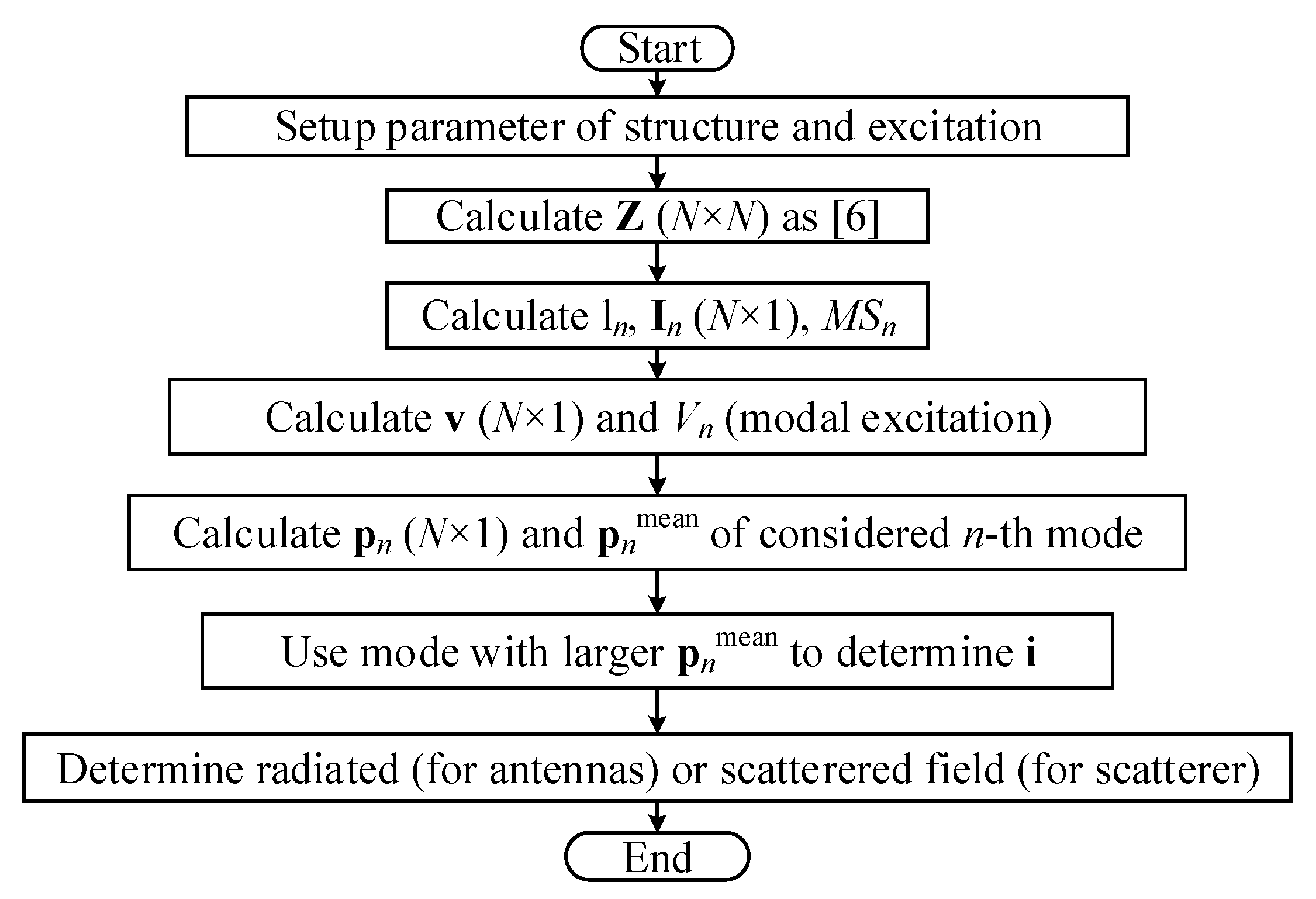
Figure 2. The dependences of I_1–9 (a), p_1–9 (b), |I| (c) and ϕ_I (d) on x along D1 and the RP of the D1 (e).

Figure 3. The dependences of I_1–3 (a), p_1–3 (b), |I| (c) and ϕ_I (d) on x along D2 and the scattered field of D2 (e).

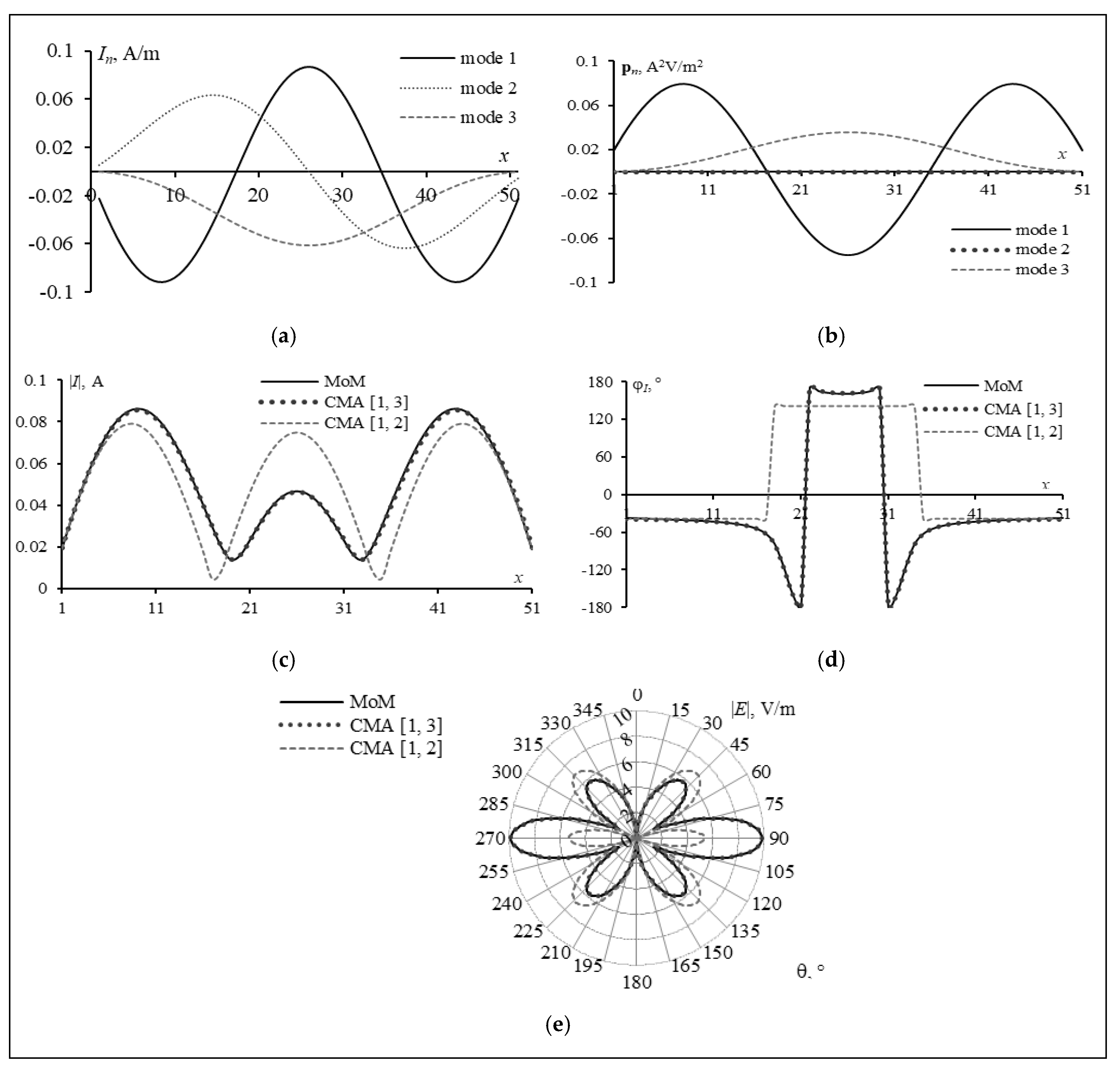
Figure 4. The dependences of |I| (a), ϕ_I (b) on x along SP and the scattered field for SP in the ϕ=90° (c) and θ=90° (d) planes when θ^inc=ϕ^inc=90°.

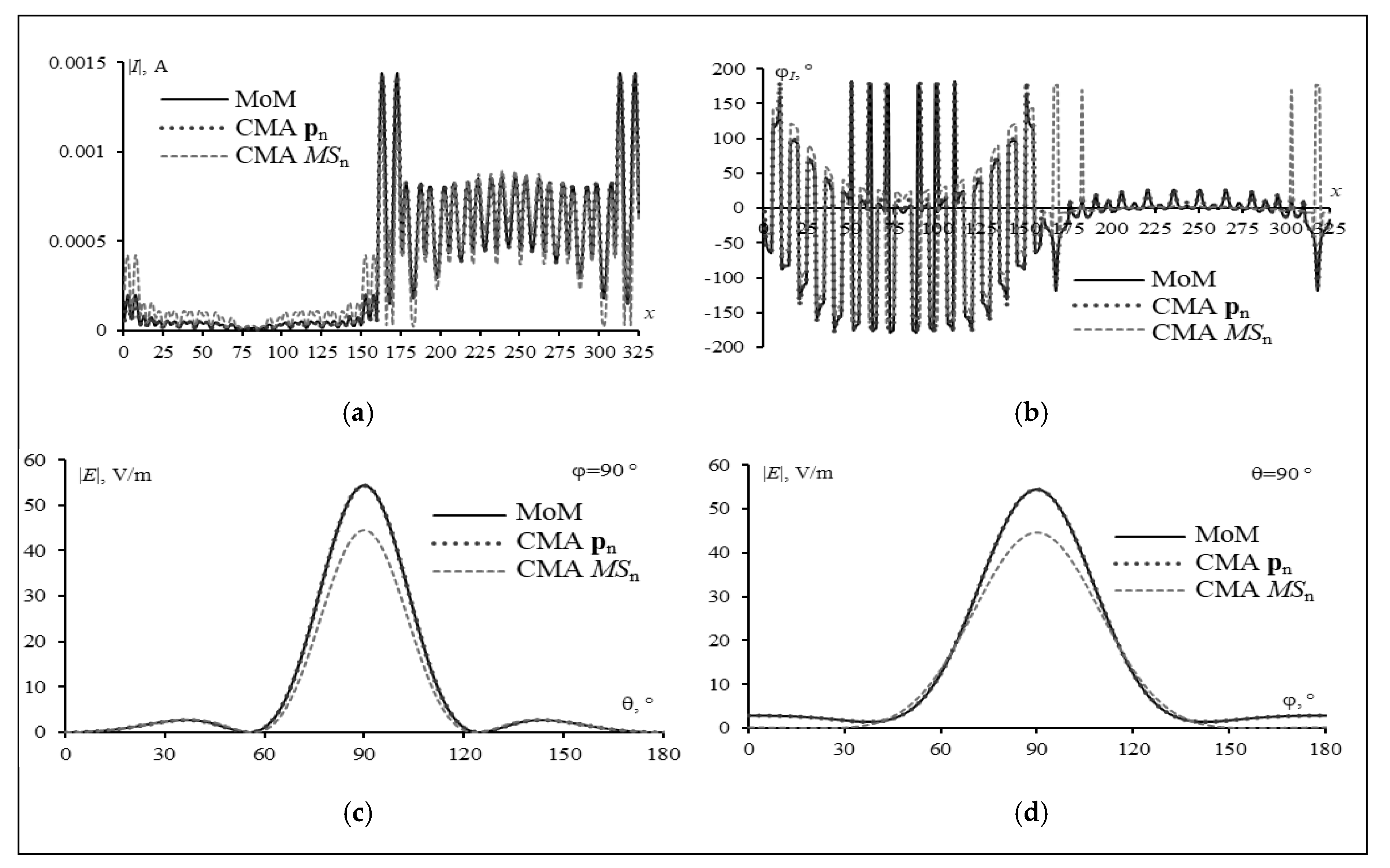
Figure 5. The algorithm that improves accuracy and computational resources in antennas and scatterers analyses using CMA.

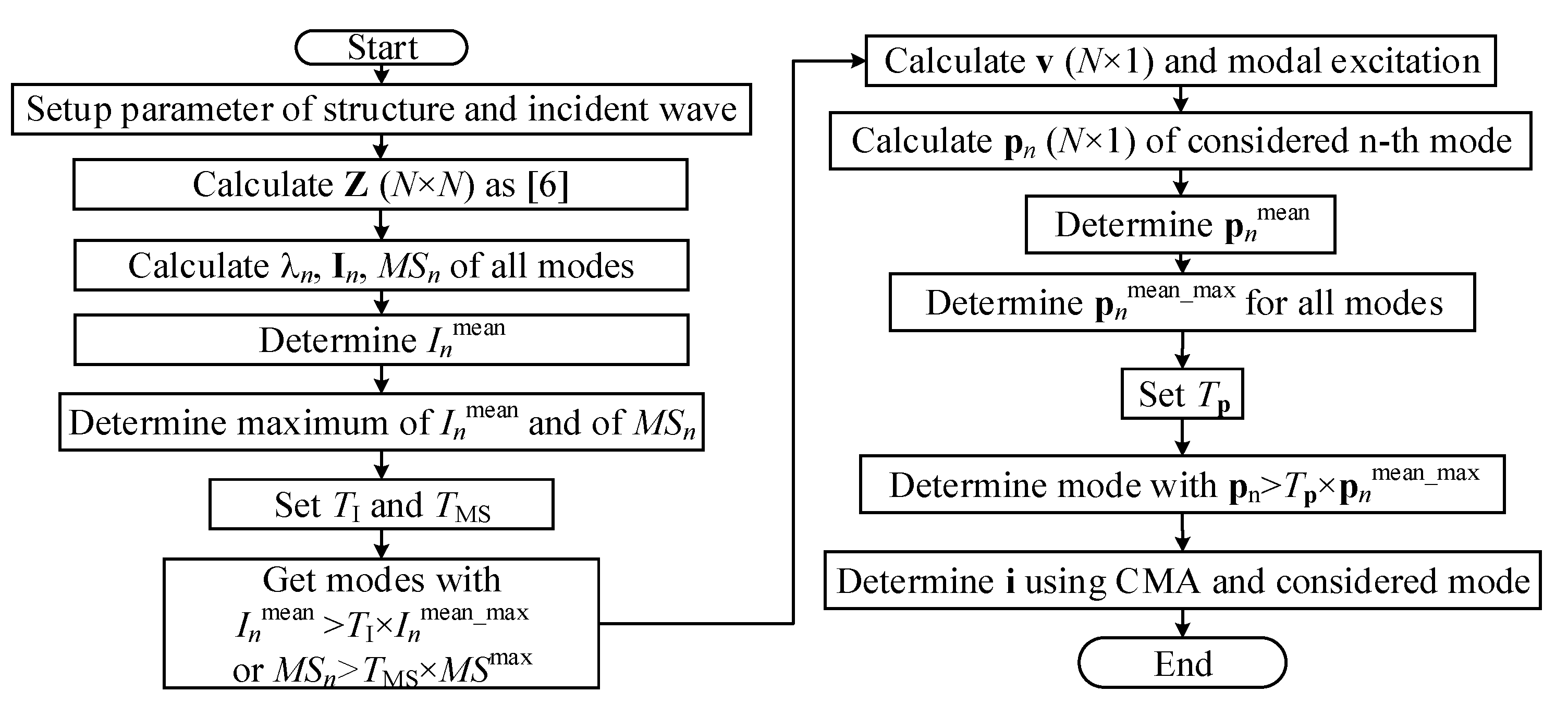
Figure 6. The equivalent WG of a solid perfectly conducting DCR (a) and TTCR (b) structures.

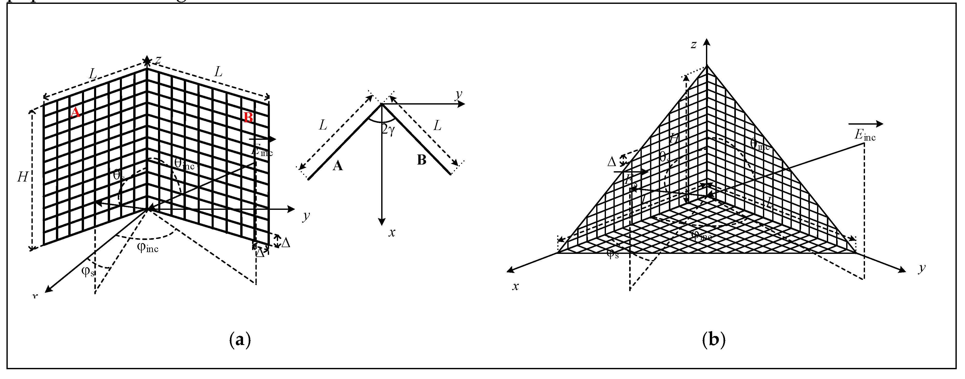
Figure 7. The measured and calculated BSCS results for S1 in the xOy (a) and yOz (b) planes.

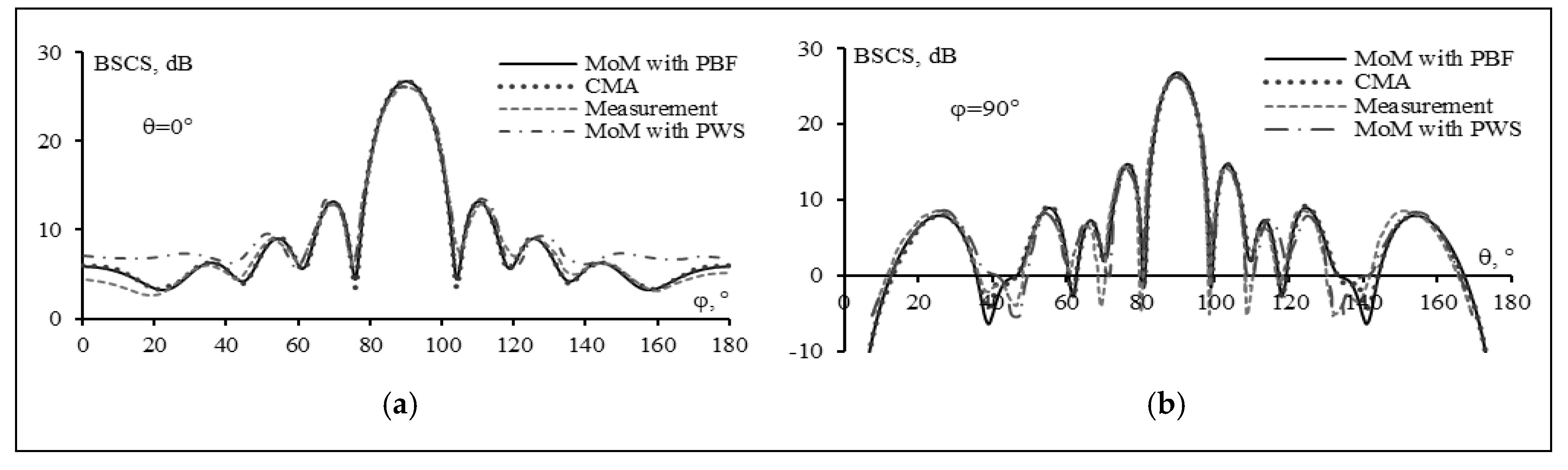
Figure 8. The measured and calculated BSCS results for S2 in the xOy (a) and yOz (b) planes.

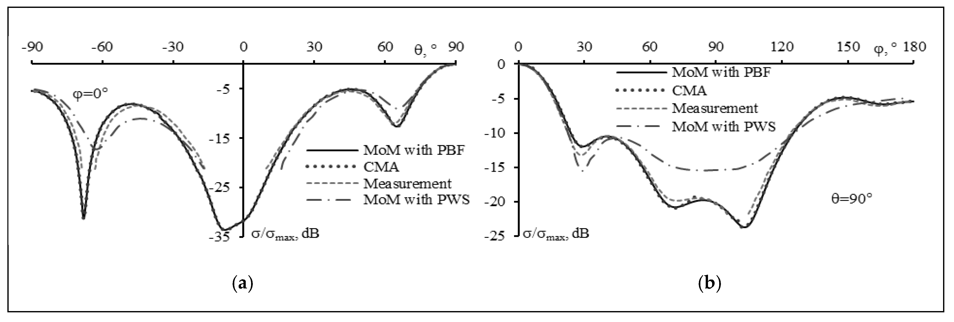
Figure 9. The measured and calculated BSCS results for S3 (a) and S4 (b) in the θ=90° plane.

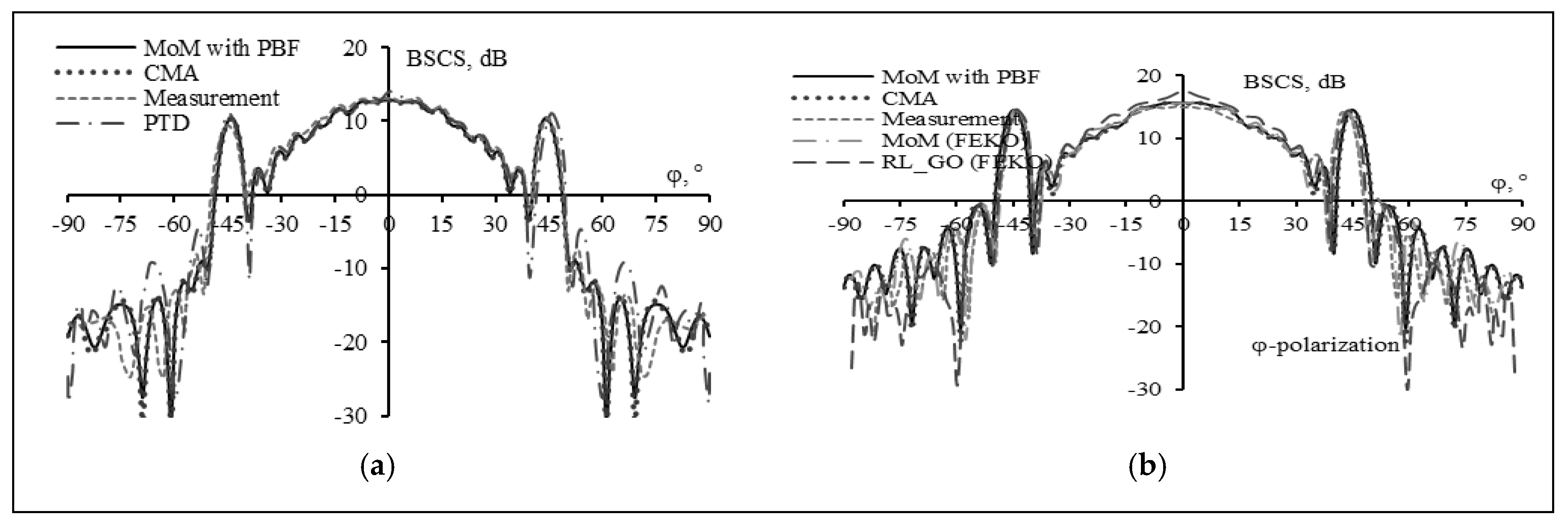
Figure 10. The calculated BSCS results for S5 in the ϕ=45° plane.

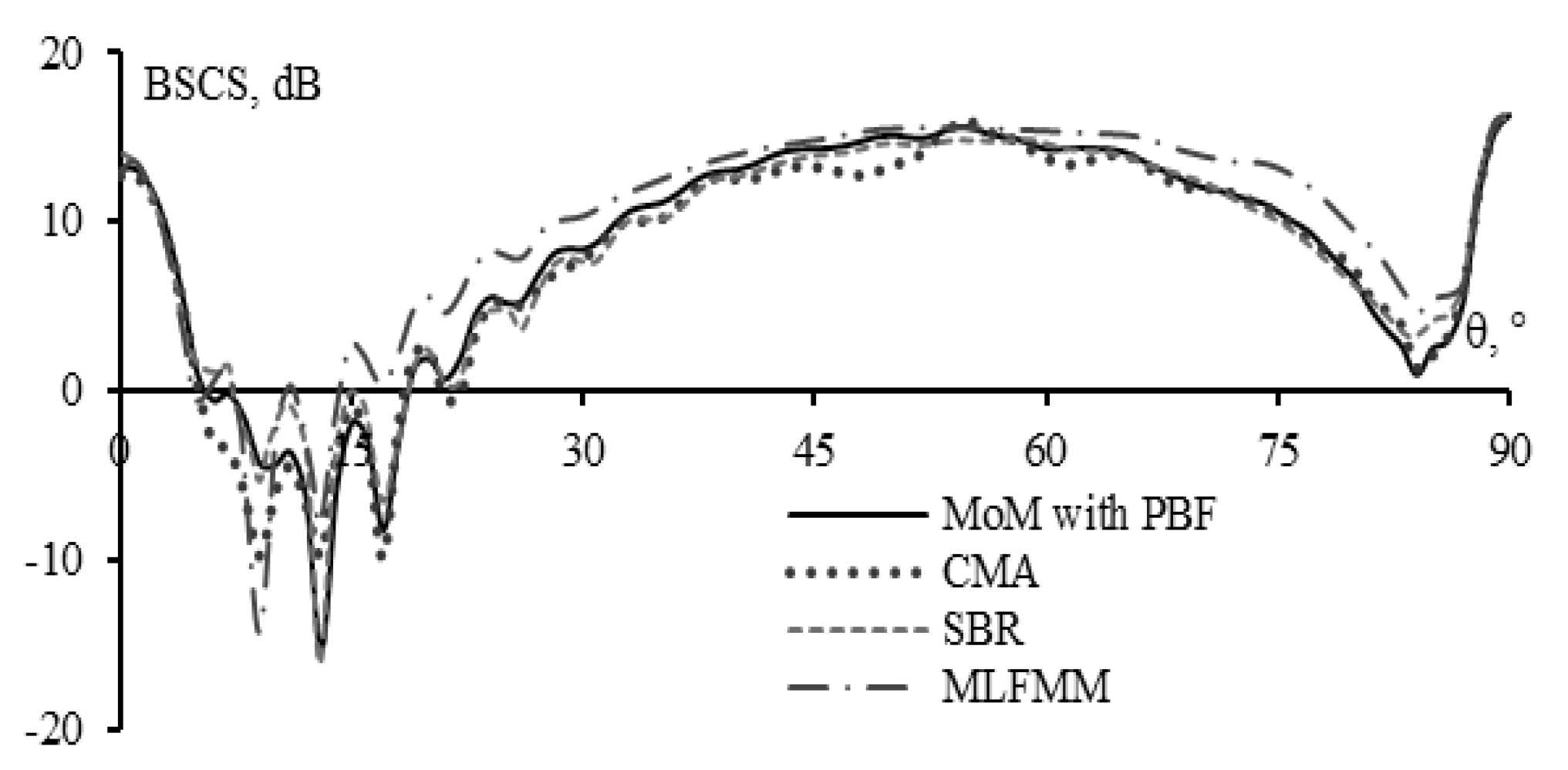
Table 1. Parameters of the structures under consideration and the incident wave used in analyses.

Structure	Size		Number of cells	Number of segments	Polarization	φ^inc, °	θ^inc, °	f, GHz	Analysis methods
	H, m	L, m
Plate [11]	3	2	30×20	1250	θ	0…180°	90°	0.3	MoM-PWS / experiment
						90°	0…180°
DCR [11]	1	0.5	20×10	840	θ	0	–90…90°	0.3	MoM-PWS / experiment
						–180°…0	90°
DCR [12]	0.18	0.18	33×33×33	4455	θ	–90…90°	90°	9.4	PTD / experiment
DCR [13]	0.3	0.3	60×60×60	14580	ϕ	–90…90°	90°	5	MoM / RL_GO / experiment
TTCR [14]	0.3	0.3	70×70×70	14910	θ	45°	0…90°	10	SBR / MLFMM

Table 2. Computational cost required to analyze different scatterers by CMA.

Structure	φ^inc, °	θ^inc, °	Time, s			Memory, MB
Structure	φ^inc, °	θ^inc, °	T_I=T_MS=0, T_p=0	T_I=T_MS=0, T_p=0.1	T_I=T_MS=0.01, T_p=0.1	T_I=T_MS=0, T_p=0	T_I=T_MS=0, T_p=0.1	T_I=T_MS=0.01, T_p=0.1
S1	0…180°	90°	667	21	20	25	20	10
S1	90°	0…180°	670	19	19	24	17	11
S2	0°	–90…90°	231	7	6	13	6	2
S2	–180…0	90°	227	7	7	12	7	3
S3	–90…90°	90°	24138	679	651	431	279	168
S4	–90…90°	90°	935064	6257	5824	3943	2521	1443
S5	45°	0…90°	478584	20226	18331	4133	3043	2504

Disclaimer/Publisher’s Note: The statements, opinions and data contained in all publications are solely those of the individual author(s) and contributor(s) and not of MDPI and/or the editor(s). MDPI and/or the editor(s) disclaim responsibility for any injury to people or property resulting from any ideas, methods, instructions or products referred to in the content.

© 2025 by the authors. Licensee MDPI, Basel, Switzerland. This article is an open access article distributed under the terms and conditions of the Creative Commons Attribution (CC BY) license (http://creativecommons.org/licenses/by/4.0/).

Copyright: This open access article is published under a Creative Commons CC BY 4.0 license, which permit the free download, distribution, and reuse, provided that the author and preprint are cited in any reuse.