
Submitted:
22 October 2025
Posted:
23 October 2025
You are already at the latest version
Abstract
This investigation examines the efficacy of the Time Series Informer (TSI) architecture in forecasting stock prices, positioning it as a pivotal instrument within business intelligence (BI) paradigms. Amid the escalating intricacy and nonlinear dynamics inherent to financial markets, deep learning frameworks have emerged as preeminent modalities for delineating sequential dependencies. Employing a comprehensive historical dataset of stock prices sourced from Google, the present analysis juxtaposes the TSI with the Long Short-Term Memory (LSTM) model. Performance is rigorously benchmarked through dual quantitative indices: The Root Mean Square Error (RMSE) and the Pearson correlation coefficient. Supplementary assessments encompass convergence trajectories, computational parsimony, and temporal overheads associated with model training. Empirical findings substantiate the superior predictive fidelity and correlative fidelity of TSI vis-à-vis LSTM, underscoring its adeptness at encapsulating protracted temporal interdependencies in financial chronologies. Visualization of convergence profiles evinces accelerated and more resilient optimization dynamics for TSI. Collectively, this multifaceted juxtaposition elucidates the model's viability for pragmatic stock market prognostication, thereby illuminating the transformative prospective of advanced neural architectures in fortifying strategic business intelligence infrastructures.
Keywords:
deep learning
; stock market
; informer
; transformers
; LSTM
1. Introduction
Financial markets are among the most complex and dynamic systems in the world, characterized by nonlinearity, high volatility, and intricate dependencies on various socio-economic factors. Accurately predicting stock prices remains a holy grail in financial analysis, with implications for investors, portfolio managers, and policy-makers. Traditionally, statistical models like ARIMA, GARCH, and linear regression have been employed to forecast prices; however, these often fall short in capturing nonlinear patterns and intricate temporal relationships inherent in stock data. Therefore, advent of AI, which is a step forward from numerical and mathematical concept to stochastically context, has changed our world economically as well as computationally (Moazezi Khah Tehran et al. 2025). In recent years, deep learning models, especially Recurrent Neural Networks (RNNs) (Mienye et al. 2024, Tariq et al. 2023) and their variants like Long Short-Term Memory (LSTM), have shown remarkable success in modeling sequential data due to their ability to retain information over long periods (Nguyen-Trang et al. 2025; Tuhin et al. 2025). RNNs, while historically significant, are often limited by the vanishing gradient problem, making them less suitable for long-term dependencies. LSTM models, with their specialized architecture containing memory cells and gating mechanisms, overcome these limitations (Hafshejani et al. 2025).
The main downside of the Long Short-Term Memory (LSTM) method is that it is computationally expensive and difficult to train due to its complex architecture, which includes multiple gates and parameters. This complexity leads to longer training times and higher resource consumption compared to simpler models or modern alternatives such as Transformers. LSTMs also struggle with capturing very long-term dependencies when sequences become extremely long, and they can be sensitive to hyperparameter choices and initialization. Additionally, because they process data sequentially, LSTMs are less parallelizable, making them less efficient for large-scale or real-time applications (Kim and Kim 2024).
The transformer architecture, introduced in 2017, revolutionized sequence modeling by supplanting recurrence with self-attention mechanisms, which parallelize computations and adeptly discern global dependencies irrespective of distance. In time series domains, transformers have supplanted RNNs in tasks requiring multivariate forecasting, with empirical validations showing marginal yet consistent gains in absolute price prediction for electronic trading scenarios. Comparative analyses further illuminate these dynamics: while LSTMs excel in resource-constrained environments for short-term horizons, transformers, including gated recurrent unit (GRU) hybrids, outperform in trend classification for equities like Tesla, leveraging attention to mitigate overfitting on noisy inputs. However, vanilla transformers suffer from prohibitive memory footprints in long-sequence regimes, prompting innovations like the Informer model.
Developed as an efficient ProbSparse self-attention variant, the Informer (or TSI herein) distills transformer efficacy for long-sequence time-series forecasting by curtailing query-key interactions to dominant elements, achieving linear complexity and up to 90% reduction in training latency compared to baselines. Its generative-style decoder further bolsters multi-step predictions, rendering it apt for financial chronologies where foresight beyond immediate horizons informs BI-driven hedging and allocation. Applications in finance have proliferated: Informer has been hybridized with empirical mode decomposition for denoising volatility surfaces in option pricing, yielding superior mean absolute errors over LSTM counterparts, and extended to multi-source integrations for meteorological-financial forecasting, though challenges persist in hyperparameter sensitivity and interpretability within opaque market microstructures. Recent enhancements, such as diffusion-augmented Informers, address distributional shifts in extreme events, amplifying its utility in stress-tested BI pipelines.
Despite these strides, a lacuna endures in the literature: while isolated deployments of Informer in financial contexts abound, rigorous, head-to-head benchmarking against entrenched models like LSTM, framed explicitly through a BI lens, remains sparse. Extant reviews aggregate hybrid DL paradigms but seldom dissect efficiency trade-offs in production-grade stock prediction, overlooking convergence stability and correlative fidelity as proxies for BI integrability. Moreover, evaluations often confine to synthetic or curtailed datasets, neglecting comprehensive historical corpora like Google stock prices, which embody tech-sector idiosyncrasies such as earnings-driven surges and algorithmic trading artifacts. This oversight hampers the translation of DL innovations into actionable BI artifacts, where not only accuracy but also parsimony and resilience under stochastic perturbations dictate adoption.
To bridge this void, the present study systematically appraises the TSI model’s efficacy for stock market prediction, juxtaposing it against LSTM within a BI-oriented framework. Leveraging a granular historical dataset of Google (Alphabet Inc.) stock prices, spanning daily closes, volumes, and adjacencies from 2004 onward, we benchmark predictive fidelity via root mean square error (RMSE) and Pearson correlation coefficient, augmented by assays of convergence trajectories, computational overheads, and training epochs. Our hypotheses posit TSI’s preeminence in encapsulating long-range dependencies, evinced by steeper learning curves and heightened correlation with empirical trajectories, thereby affirming its salience for scalable BI deployments.
The manuscript unfolds as follows: Section 2 delineates the theoretical underpinnings of TSI and LSTM, alongside dataset curation, as well as encompassing hyperparameter tuning and validation protocols. Section 3 proffers empirical results, replete with visualizations of performance metrics. Concluding remarks synthesize contributions and prospective trajectories.
2. Materials and Methods
2.1. Data Description and Preparation
The dataset employed comprises historical daily closing prices of Google (GOOGL), available via Yahoo Finance. This dataset spans roughly a decade, providing a rich temporal sequence for modeling. Importantly, stock prices are influenced by multifaceted factors; however, for the scope of this study, we focus purely on historical close prices to assess the models’ ability to learn temporal dependencies. The dataset is depicted in Figure 1. Data preprocessing begins with normalization through MinMaxScaler to compress values into the [0,1] range, facilitating stable training. We then truncate the series into sequences of length 60 days, where each sequence predicts the subsequent day’s price. This windowing approach is their standard in time series deep learning applications. The dataset is split into training and testing subsets, with 80% allocated for training to enable robust learning, and the remaining 20% used for evaluation and comparison. The sequences are reshaped appropriately to fit into the models, with each sample being a 3D tensor: (samples, timesteps, features).
2.2. LSTM Model
The LSTM model incorporates an LSTM layer with 50 units, favored for its gating mechanisms that mitigate vanishing gradient issues, followed by the Dense output. The model is compiled with the Adam optimizer, a popular choice for time series forecasting, employing Mean Squared Error (MSE) as the loss function. Figure 2 depict the individual architectures of the LSTM model, illustrating the flow of data and gating mechanisms.
2.2.1. Hyperparameters of the LSTM Network
The LSTM model is configured with the following hyperparameters: input_size=1 (for the univariate close price feature), hidden_size=50 (number of units in each LSTM layer), num_layers=2 (stacked LSTM layers for capturing complex dependencies), output_size=1 (for predicting the next close price), learning_rate=0.001 (for the Adam optimizer), epochs=50 (training iterations), batch_size=32 (mini-batch size for efficient gradient updates), and MSELoss as the loss function (mean squared error for regression tasks). These parameters balance model capacity and computational efficiency, with the 2-layer structure enabling hierarchical pattern learning in time series data.
2.2.2. LSTM Architecture
The architecture consists of a stacked LSTM network followed by a linear output layer. Input sequences (shape: batch size × sequence length × 1) are processed through two LSTM layers, where each layer updates the hidden state ht and cell state Ct using forget, input, and output gates to mitigate vanishing gradients and capture long-term dependencies. The final hidden state from the second layer is passed to a fully connected linear layer for single-value prediction. The diagram below illustrates a single LSTM unit in the chain, showing recurrent connections for input Xt, hidden state ht, and cell state Ct, with gates (σ for sigmoid, tanh for hyperbolic tangent) controlling information flow
2.3. Time Series Informer (TSI)
Transformer neural networks (Vaswani 2017) are machine learning models proposed mainly to overcome LSTM drawbacks. The concept of this method is the attention not only to the events that occur before a specific predictand, but also to the events that happen after it. This concept has attracted much attention from researchers and scientists in many research areas, such as information retrieval, text classification, and document summarization. In addition to language related applications, Transformers have also been utilized in computer vision (Nicolas et al. 2020), chemistry (Schwaller et al. 2019), life sciences (Rives et al. 2016), and river level prediction (Castangia et al. 2023). Transformer method suffers from some drawbacks. For example, the skill of the method for sharp changes is relatively low (Ye et al. 2022). Inspired by the works of Zhou et al. (2021) and Naisipour et al. (2025a) we feed long-term ENSO time series into the Informer network and receive a two years long prediction. The overall architecture of Informer network , as shown in Figure 3, consists of five main components.
Given a time sequence at time t and the output corresponding sequence , the module encodes the input representations into a hidden state representation and decodes an output representations from . The extracted features of each series are added to the positional encoders, after the input series have been embedded and representative features have been created by the embedding module. We consider that we have t-th sequence input and p types of global time stamps and the feature dimension after input representation is . We first use a fixed position embedding to maintain the local context:
where . A learnable stamp embedding utilizes every global time stamp with limited vocab size. Since the self-attention’s similarity computation can have access to global context, the computation consuming is affordable on long inputs. we project the scalar context into -dim vector with 1-D convolutional filters with kernel width equal to 3 and stride one to align the dimension. Thus, we have the feeding vector:
In this equation, is the factor balancing the magnitude between the scalar projection and local/global embedding that is set to 1 in this study, and .
ProbSparse Self-attention. We apply the ProbSparse self-attention by allowing each key to only attend to the u dominant queries:
where Q is a sparse matrix of the same size of q and it only contains the Top-u queries under the sparsity measurement .
Encoder. The encoder’s purpose is to extract from the lengthy sequential inputs the reliable long-range dependency. As the input representation is done, the matrix will be the new shape of the t-th sequence input .
Self-attention Distilling. We use the distilling operation to privilege the superior ones with dominating features, because the natural consequence of the ProbSparse self-attention mechanism has redundant combinations of value . This also makes a focused self-attention feature map in the next layer. Observing the n-heads weights matrix of the Attention blocks in Figure 4, it drastically reduces the input’s time dimension. According to Equation (6), the applied procedure forwards from j-th layer into (j + 1)-th layer.
In this formula, represents the attention block, is the activation function and is an 1D convolutional filter with kernel width of three. To reduces the whole memory usage, a max-pooling layer with stride 2 down samples into its half slice.
Decoder. We use a stack of two identical multi-head attention layers as the decoder, and to alleviate the speed plunge in long prediction, we apply the generative inference. The following vectors are given to the vanilla decoder as the input:
where and are is the start token and placeholder for the target sequence, respectively. The final layer is a dense layer that generates the results. Table 1 is a detailed description of the TSI model’s hyperparameters.
2.4. Generative Inference
We use one of the best data augmentation methods called Generative Adversarial Network (GAN) to increase input data that can be trained to imitate a data distribution. GAN was first proposed in 2014 by Ian Goodfellow et al. This method learns to produce fresh data with the same statistics as the training set given a training set. GANs have shown beneficial for semi-supervised learning (Salimans et al. 2016) while being first proposed as a type of generative model for unsupervised learning. They also have been successful in fully supervised learning (Isola et al. 2017) and reinforcement learning (Ho and Ermon 2016). GANs can improve astronomical images (Schawinski et al. 2017) and simulate gravitational lensing for dark matter research. They were used to model the distribution of dark matter in the universe and to predict the occurrence of gravitational lensing (Mustafa. et al. 2019) GANs have been proposed as a fast and accurate way of modeling high-energy jet formation (Paganini et al. 2017) and modeling showers through calorimeters of high-energy physics experiments (Erdmann et al. 2019) They have also been trained to approximate bottlenecks in simulations of particle physics experiments (Salamani et al. 2018).
The GAN consist of “indirect” training through the discriminator and another neural network that can tell how “realistic” the input seems, which itself is also being updated dynamically. This means that the generator is not trained to minimize the distance to a specific image, but rather to fool the discriminator. In this study, Each probability space (Ω, μref) defines a GAN game. There are two players called generator and discriminator. The generator’s strategy set is P (Ω), the set of all probability measures μG on (Ω). The discriminator’s strategy set is the set of Markov kernels μD: Ω → P [0,1] where P [0,1] is the set of probability measures on [0,1]. The GAN game is a zero-sum game, with the objective function:
The generator aims to minimize the objective, and the discriminator aims to maximize the objective. The generative network’s training goal is to increase the error rate of the discriminative network (Luc et al. 2016; Karpathy et al. 2016). GANs are implicit generative models (Mohamed et al. 2016) that do not explicitly model the likelihood function nor provide a means for finding the latent variable corresponding to a given sample.
Start token is efficiently applied in NLP’s dynamic decoding (Devlin et al. 2018), and we extend it into a generative way. We sample a long sequence in the input sequence, so contains target sequence’s time stamp, that is the context at the target. Instead of the cumbersome “dynamic decoding” in the vanilla encoder-decoder blocks, the decoder used in this study forecasts outputs by a forward procedure. We chose the MSE loss function across the entire Informer module.
2.5. Ensembling Procedure
Ensembling constitutes a fundamental methodology in machine learning designed to enhance predictive performance and model robustness by aggregating the outputs of multiple individual models (Ganji et al. 2025a). Rather than relying on a single estimator, ensemble approaches, such as bagging, boosting, and stacking, leverage the diversity and complementary strengths of multiple learners to mitigate variance, reduce bias, and improve generalization (Naisipour et al. 2024a). This paradigm capitalizes on the premise that aggregated predictions often outperform any constituent model, particularly in complex domains characterized by high variability or nonlinear interactions, such as financial time series forecasting or climatic phenomena (Naisipour et al. 2024b). By synthesizing multiple model inferences, ensembling not only stabilizes predictions against stochastic fluctuations due to random initialization or data sampling but also attenuates the risk of overfitting (Ganji et al. 2025b).
In the present investigation, an ensemble-based approach was employed to further refine the predictive accuracy of both the TSI and LSTM architectures inspired by the study of (Naisipour et al. 2025b). Each model was independently trained ten times using distinct random weight initializations while maintaining consistent data partitions and hyperparameter configurations. The outputs from these ten individual runs were subsequently averaged to produce a single consolidated prediction for each model. This averaging strategy effectively smooths out the variability stemming from random initialization, yielding more stable and reliable forecasts. Consequently, the ensemble outputs represent a statistically more robust estimation of each model’s predictive capability, thereby ensuring a fair and reproducible comparative evaluation between TSI and LSTM frameworks.
2.6. Training Procedure
The models are trained for 20 epochs with a batch size of 32, and a validation split of 20% helps monitor overfitting and convergence. Early stopping could be incorporated, but here we seek to analyze the raw convergence behaviors.
2.7. Evaluation Metrics
In modeling and numerical simulation, ensuring fairness and accuracy through appropriate performance metrics is indispensable: only by employing reliable and interpretable error indicators can one ensure that a model performs correctly and equitably across its domain of application (Naisipour et al. 2009; Labibzadeh et al. 2008). Extending this principle to data-driven contexts, recent studies emphasize the decisive role of metric selection in evaluating deep learning convolutional neural networks, demonstrating that inappropriate metrics can distort model assessment and lead to biased interpretations of predictive skill (Labibzadeh, et al. 2015). Collectively, these studies underscore that fair model evaluation demands metrics that are rigorously derived, physically or statistically relevant, and sensitive to both global performance and local deviations; without such precision, models risk producing overconfident, biased, or misleading results that compromise scientific validity and practical applicability (Naisipour et al. 2024c).
Thus in this study, models are evaluated based on RMSE for accuracy and Pearson correlation coefficient to ascertain the strength of linear association with true prices. These metrics are calculated on the test set.
Below are the formulas for each metric and the explanation of their parameters:
Pearson Correlation Coefficient (PCC):
The PCC measures the strength and direction of the linear relationship between predicted and observed Niño 3.4 values. This metric is particularly useful for assessing the model’s ability to track the temporal dynamics events. The metric is a dimensionless one that calculates the strength and direction of the linear relationship between the predicted and observed values. Values range between -1 and +1.
Root Mean Squared Error (RMSE):
RMSE gives greater weight to larger errors by squaring the differences between predicted and actual values. This metric is useful for identifying significant outliers or instances where the model deviates substantially from observed patterns.
RMSE Unit is the same as the predicted variable. Since RMSE is the square root of MSE, it brings the metric back to the original units of the target variable, making interpretation of prediction errors easier. In these formulae, is the actual value and denotes the prediction result. Here, m is the calendar month.
The performance evaluation of the model in this study is grounded in two widely accepted metrics, each stemming from established methodologies that offer distinct perspectives on model accuracy and predictive power. The first metric, the PCC, quantifies the linear relationship between predicted and observed values, where a higher PCC value, approaching +1, reflects a strong positive correlation, indicating effective representation of the market value (Glantz and Ramirez, 2020). The RMSE calculates the square of errors before averaging, therefore emphasizing larger errors more heavily. The RMSE, derived from the square root of MSE, maintains the same unit as the original data and is particularly sensitive to large errors, thus smaller values are preferable for a well-calibrated model (Hyndman and Athanasopoulos, 2018).
3. Results
3.1. Predictive Performance and Comparison
The predicted stock prices for the test data are plotted against actual prices in Figure 5. Visual inspection reveals the TSI’s superior ability to follow long-term trends and respond to recent fluctuations compared to the standard LSTM, which often underestimates volatility. Table 2 compares the performance and training time of two models, LSTM and TSI, using three metrics: RMSE, Pearson Correlation Coefficient, and training time in seconds. The TSI model outperforms the LSTM, achieving a lower RMSE of 1.75 compared to 2.35, indicating more accurate predictions. Additionally, TSI shows a stronger linear relationship with the target data, as reflected by a higher Pearson correlation coefficient of 0.94 versus 0.88 for LSTM. Pearson correlation analysis confirms that the TSI predictions align more closely with actual stock prices. The higher correlation underscores the model’s proficiency in capturing temporal dependencies. These results demonstrate a clear advantage of TSI over the traditional LSTM in stock forecasting, aligning with existing literature. However, this improved performance comes with a longer training time, with TSI taking 60 seconds to train compared to 45 seconds for LSTM. Overall, TSI offers better accuracy and correlation but requires more computational time.
3.2. Comparison of Convergence
Plotting the training and validation loss over epochs (Figure 6) reveals that the TSI converges faster and more smoothly than the LSTM, which exhibits greater oscillations and slower convergence due to vanishing gradients.
4. Conclusions
This comprehensive comparison underscores the efficacy of deep learning architectures, particularly TSIs, in modeling complex financial time series. Our experiments have shown that TSI model not only outperforms LSTMs in predictive accuracy but also converge faster and exhibit greater stability during training. The lower RMSE and higher correlation coefficients affirm the suitability of TSIs for practical stock market prediction tasks.
The convergence analysis indicates that TSIs can learn sparse dependencies more efficiently, which is vital in financial contexts where market movements are influenced by historical patterns extending beyond short-term windows. Despite a marginal increase in computational costs, the improved accuracy and stability make TSIs attractive for deployment in business intelligence systems.
Nevertheless, this study also highlights the importance of hyperparameter tuning, the potential for integrating additional features (such as volume, technical indicators), and the need for more rigorous testing over different stocks and market conditions. This research showed that hybrid models blending attention mechanisms with convolutional layers can boost predictive capabilities.
In real-world applications, the balance between accuracy and computational efficiency must be carefully managed, especially when deploying models for high-frequency trading or risk management systems. Overall, the results reinforce the position of TSIs as a mainstay deep learning approach for stock market forecasting, fostering more informed and strategic business decisions.
References
- Castangia, M., Grajales, L., Aliberti, A., Rossi, C., 2023, Transformer neural networks for interpretable flood forecasting, Environmental Modelling & Software, Volume 160,105581.
- Das, S., Tariq, A., Santos, T., Kantareddy, S.S., Banerjee, I. (2023). Recurrent Neural Networks (RNNs): Architectures, Training Tricks, and Introduction to Influential Research. In: Colliot, O. (eds) Machine Learning for Brain Disorders. Neuromethods, vol 197. Humana, New York, NY. [CrossRef]
- Devlin, J., et al. Bert: Pre-training of deep bidirectional transformers for language understanding. arXiv:1810.04805 (2018).
- Erdmann, M., Glombitza, J., Quast, T., 2019. Precise Simulation of Electromagnetic Calorimeter Showers Using a Wasserstein Generative Adversarial Network. Computing and Software for Big Science. 3: 4. arXiv:1807.01954.
- Glantz, M.H. and Ramirez, I.J. (2020) Reviewing the Oceanic Niño Index (ONI) to Enhance Societal Readiness for El Niño’s Impacts. International Journal of Disaster Risk Science, 11, 394-403. [CrossRef]
- Goodfellow, I. J et al. 2004. Elasto-plastic fracturing model for wellbore stability using non-penetrating fluids. arXiv, 10.48550/ARXIV.1406.2661.
- Hafshejani, M.S., Mansouri, N. Enhancing Stock Market Prediction with LSTM: A Review of Recent Developments and Comparative Analysis. Arch Computat Methods Eng (2025). [CrossRef]
- Ho, J., Ermon, S. 2016. Generative Adversarial Imitation Learning”. Advances in Neural Information Processing Systems. 29: 4565–4573. arXiv:1606.03476. Bibcode:2016arXiv160603476H.
- Hyndman, R.J. and Athanasopoulos, G. (2018) Forecasting: Principles and Practice. OTexts.
- Isola, P., Zhu, J., Zhou, T., Efros, A., 2017, Image-to-Image Translation with Conditional Adversarial Nets. Computer Vision and Pattern Recognition.
- Karpathy, A., et al. 2016, Generative Models, OpenAI.
- Kim, E., Kim, Y. Exploring the potential of spiking neural networks in biomedical applications: advantages, limitations, and future perspectives. Biomed. Eng. Lett. 14, 967–980 (2024). [CrossRef]
- Labibzadeh, M., et al., (2015). Efficiency Test of the Discrete Least Squares Meshless Method in Solving Heat Conduction Problems Using Error Estimation. Sharif: Civil Enineering, 31-2(3.2), 31-40. Sid. Https://Sid.Ir/Paper/127886/En.
- Labibzadeh, et al., (2008). An Assessment of Compressive Size Effect of Plane Concrete Using Combination of Micro-Plane Damage Based Model and 3D Finite Elements Approach. American Journal of Applied Sciences, 5(2), 106-109. [CrossRef]
- Luc, P., et al., 2016. Semantic Segmentation using Adversarial Networks. NIPS Workshop on Adversarial Training, Dec, Barcelona, Spain. arXiv:1611.08408. Bibcode:2016arXiv161108408L.
- Mienye, I. D., Swart, T. G., Obaido G.,(2024). Recurrent neural networks: A comprehensive review of architectures, variants, and applications, Information 15 (9), 517.
- Moazezi Khah Tehran, A., Hassani, A., Mohajer, S., Darvishan, S., Shafiesabet, A., & Tashakkori, A. (2025). The Impact of Financial Literacy on Financial Behavior and Financial Resilience with the Mediating Role of Financial Self-Efficacy. International Journal of Industrial Engineering and Operational Research, 7(2), 38-55. [CrossRef]
- Mohamed, S., Lakshminarayanan, B. 2016. Learning in Implicit Generative Models. arXiv:1610.03483.
- Mustafa, M., et al. 2019. CosmoGAN: creating high-fidelity weak lensing convergence maps using Generative Adversarial Networks. Computational Astrophysics and Cosmology. 6 (1): 1. arXiv:1706.02390. ISSN 2197-7909.
- Naisipour, M., Afshar, M. H., Hassani, B., Zeinali, M., 1388, (2009), An error indicator for two-dimensional elasticity problems in the discrete least squares meshless method,8th International Congress on Civil Engineering,Shiraz, https://civilica.com/doc/62892.
- Naisipour, M., Saeedpanah, I., Adib, A., Neysipour, M. H., Forecasting El Niño Six Months in Advance Utilizing Augmented Convolutional Neural Network, (2024), 14th International Conference on Computer and Knowledge Engineering (ICCKE), Mashhad, Iran, Islamic Republic of, 2024, pp. 359-364, . [CrossRef]
- Naisipour, M., Ganji, S., Saeedpanah, I., Mehrakizadeh, B., Adib, A., Novel Insights in Deep Learning for Predicting Climate Phenomena, (2024), 14th International Conference on Computer and Knowledge Engineering (ICCKE), Mashhad, Iran, Islamic Republic of, 2024, pp. 314-325, . [CrossRef]
- Naisipour, M., Saeedpanah, I., & Adib, A., Novel deep learning method for forecasting ENSO. Journal of Hydraulic Structures, 14-25 (2024). DOI: . [CrossRef]
- Naisipour, M., Saeedpanah, I. & Adib, A. Multimodal Deep Learning for Two-Year ENSO Forecast. Water Resour Manage 39, 3745–3775 (2025). [CrossRef]
- Naisipour, M., Saeedpanah, I., & Adib, A., Metrics matters: A deep assessment of deep learning CNN method for ENSO forecast, Atmospheric Research, (2025), 108545, ISSN 0169-8095, . [CrossRef]
- Nguyen-Trang, T., Lethi-Thu, T. & Vo-Van, T. Interval-Valued Time Series Prediction for Vietnam Stock Indicators Based on Ensemble Long Short-Term Memory Networks. Comput Econ (2025). [CrossRef]
- Nicolas, C., Francisco, M., Gabriel, S., Nicolas, U., Alexander, K., Sergey, Z., 2020, End-to-end object detection with transformers, Proceedings of ECCV, pp. 213-229.
- Paganini, M., de Oliveira, L., Nachman, B. 2017. Learning Particle Physics by Example: Location-Aware Generative Adversarial Networks for Physics Synthesis. Computing and Software for Big Science. 1: 4. arXiv:1701.05927. doi:10.1007/s41781-017-0004-6.
- Rives A., Meier J., Sercu T., Goyal S., et al., 2016, Biological structure and function emerge from scaling unsupervised learning to 250 million protein sequences, Proc. Natl. Acad. Sci., 118 (15), 10.1073/pnas.2016239118.
- Ganji, S., Labibzadeh, A. R., Hassani, A., et al., (2025) Leveraging GNN to Enhance MEF Method in Predicting ENSO. arXiv preprint arXiv:2508.07410v3. [CrossRef]
- Ganji, S., Naisipour, M., Hassani, A., Adib, A., (2025) Distillation of CNN Ensemble Results for Enhanced Long-Term Prediction of the ENSO Phenomenon. arXiv preprint arXiv:2509.06227. [CrossRef]
- Salamani, D., et al., 2018, Deep generative models for fast shower simulation in ATLAS. IEEE 14th International Conference on e-Science, pp. 348-348.
- Salimans T., et al. 2016. Improved Techniques for Training GANs. arXiv:1606.03498.
- Schawinski, K., et al., 2017. Generative Adversarial Networks recover features in astrophysical images of galaxies beyond the deconvolution limit. Monthly Notices of the Royal Astronomical Society: Letters. 467 (1): L110–L114.
- Schwaller P., Laino T., Gaudin T., Bolgar P., Hunter C., Bekas C., Lee A., 2019, Molecular transformer: A model for uncertainty-calibrated chemical reaction prediction, ACS Central Sci., 5 (9), pp. 1572-1583.
- Tuhin, K.H., Nobi, A., Rakib, M.H. et al. Long short-term memory autoencoder based network of financial indices. Humanit Soc Sci Commun 12, 100 (2025). [CrossRef]
- Vaswani A., Shazeer N., Parmar N., et al., 2017, Attention is all you need, Proceedings of NeurIPS, pp. 5998-6008.
- Ye, F., Hu, J., Huang, T., You, L., Weng, B., Gao, J., 2022, Transformer for EI Niño-Southern Oscillation Prediction, IEEE Geoscience and Remote Sensing Letters, vol. 19, pp. 1-5.
- Zhou, H., Zhang, S., et al. Informer: Beyond Efficient Transformer for Long Sequence Time-Series Forecasting. AAAI-21 (2021).
Figure 1.
stock prices used to evaluate models.
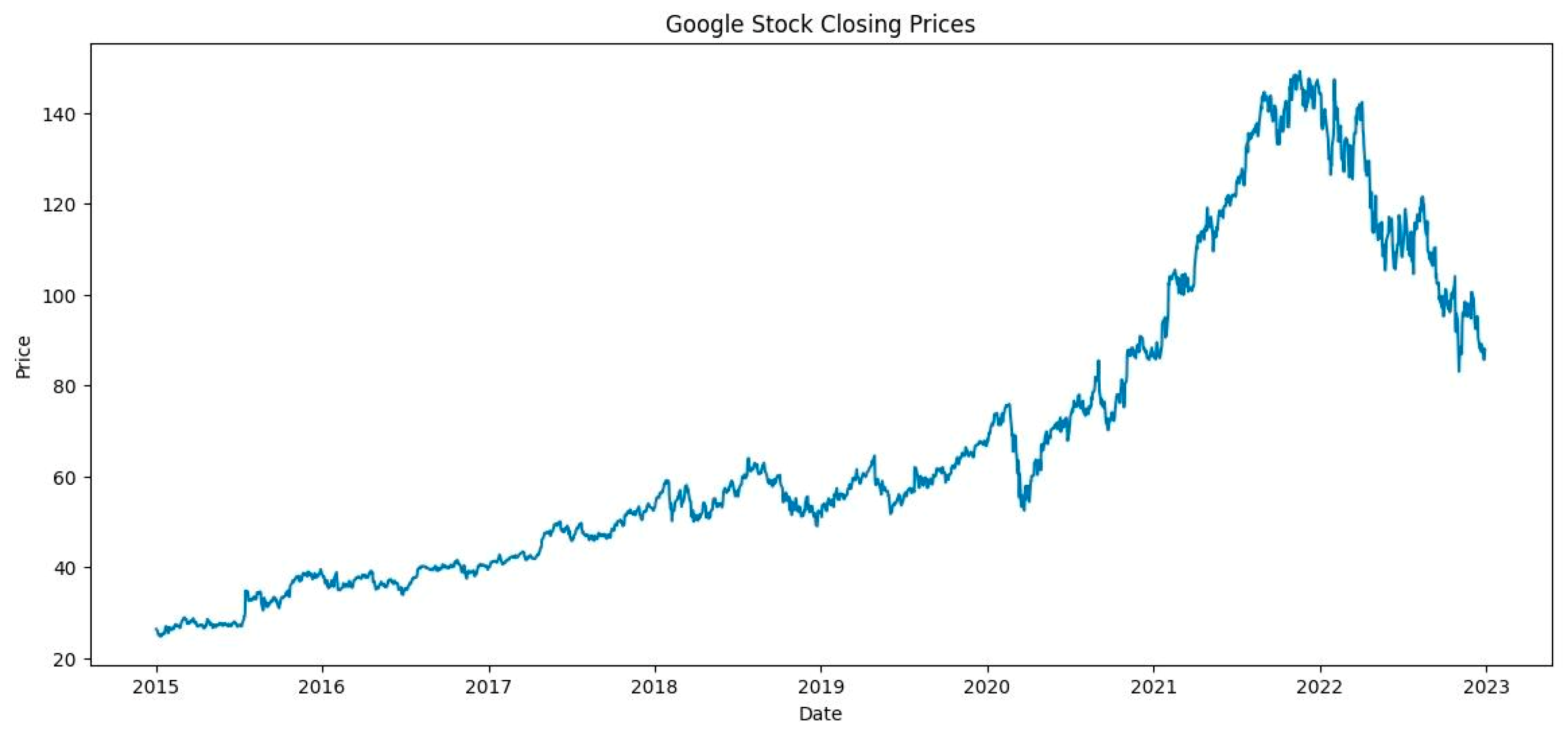
Figure 2.
LSTM model architecture.
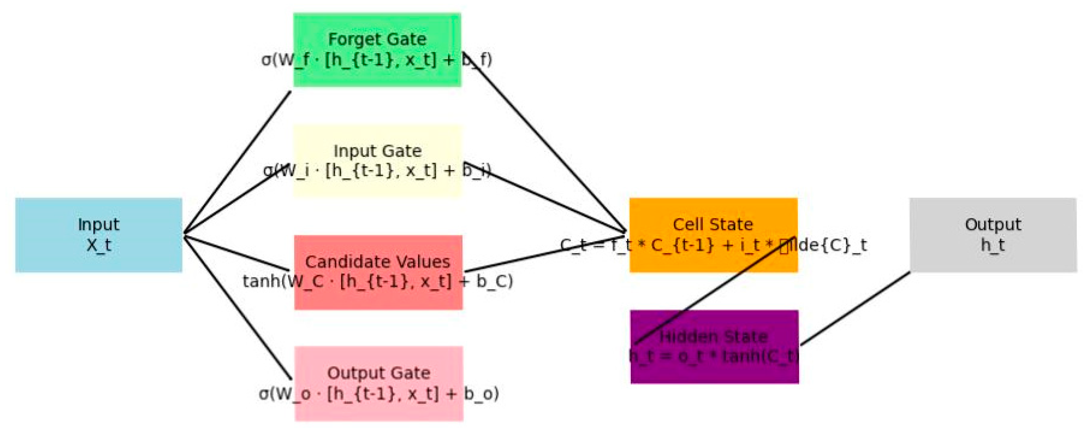
Figure 3.
Overall view of Informer Model.
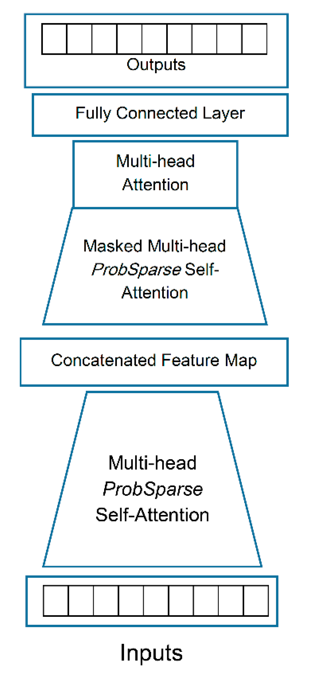
Figure 4.
The encoder’s single stack in the Informer module.
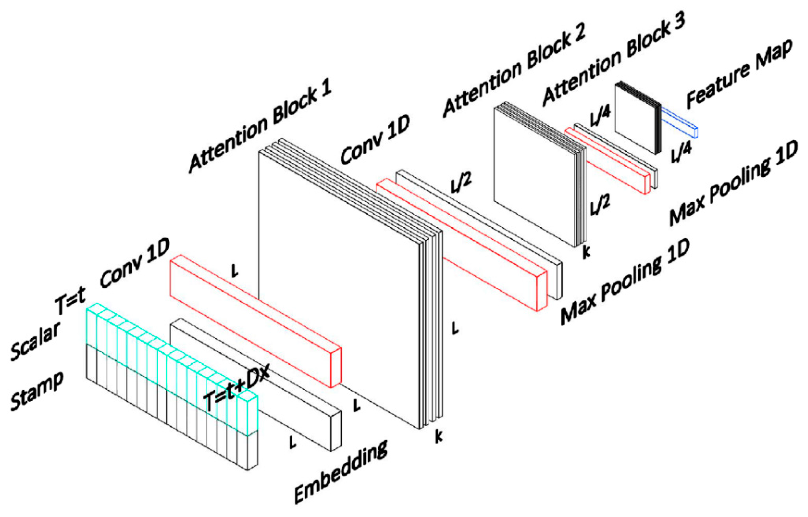
Figure 5.
The predicted stock prices for the test data are plotted against actual prices.
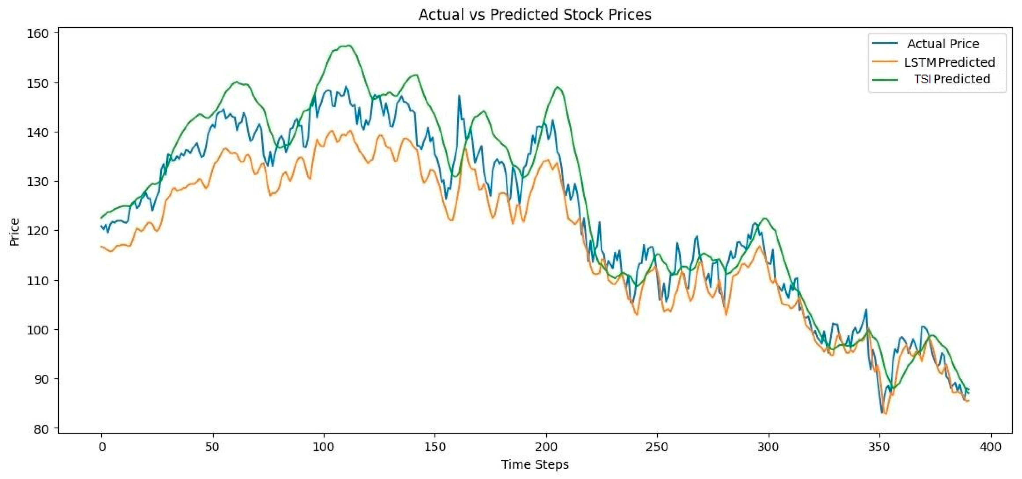
Figure 6.
Convergence Plots of Loss over Epochs.
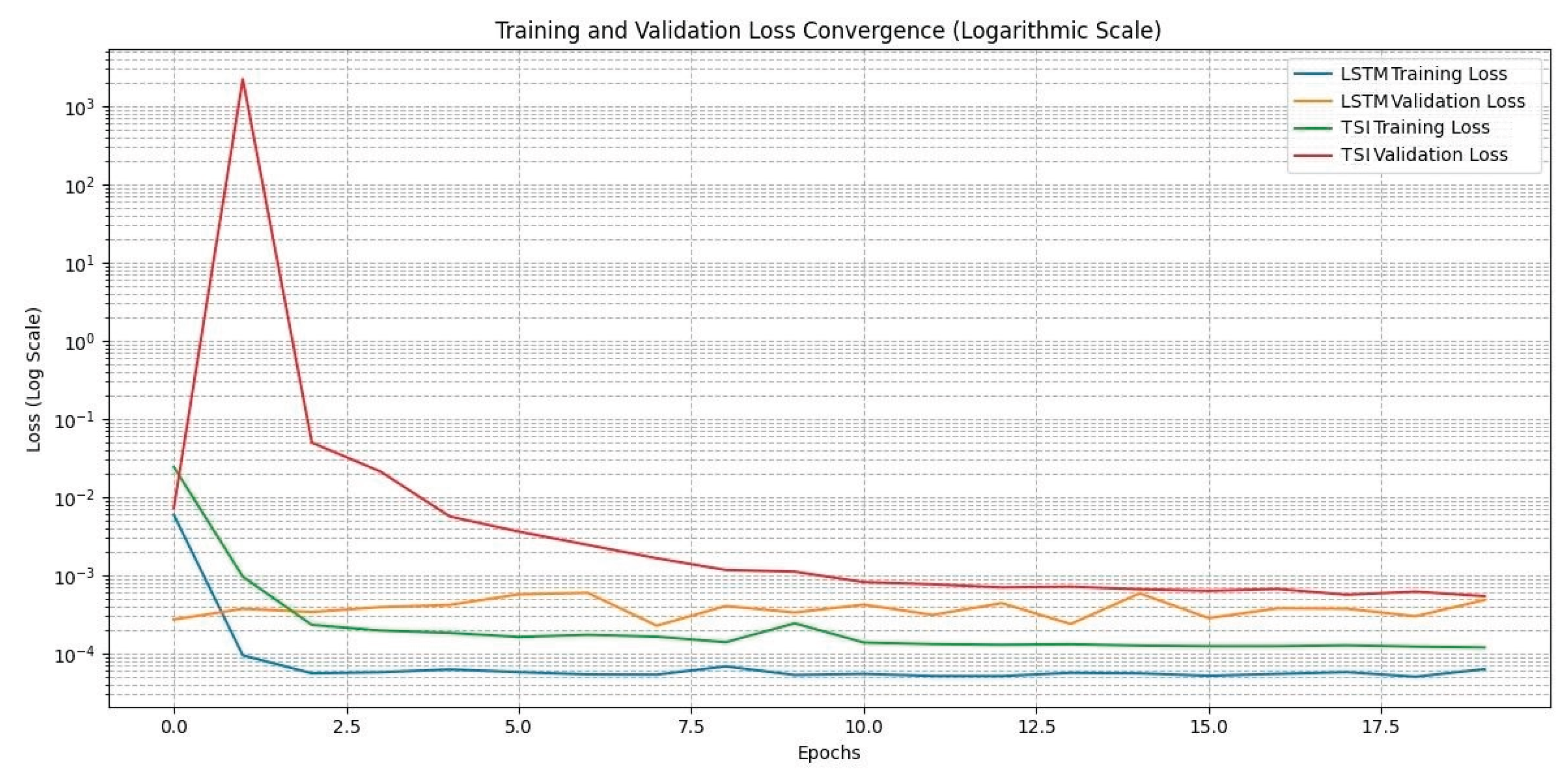

Table 1.
Hyper parameters of the TSI module.
| Input sequence length of the Informer encoder | 48 |
| Start token length of the Informer decoder | 24 |
| Encoder input size | 7 |
| Decoder input size | 7 |
| Probsparse attention factor | 5 |
| Dimension of the model | 128 |
| Number of heads | 8 |
| Number of encoder layers | 2 |
| Number of decoder layers | 1 |
| Dropout | 0.04 |
| Attention used in the encoder | Prob sparse |
| Time features encoding | fixed |
| Activation function | RELU |
| Whether to use distilling in the encoder | True |
| Padding | 0 |
| Batch size | 80 |
| Learning rate | 0.001 |
| Loss function | MSE |
| Ensemble Numbers | 10 |
Table 2.
Models’ performance and training time.
| Model | RMSE | Pearson Correlation Coefficient | Training Time (seconds) |
| LSTM | 2.35 | 0.88 | 45 |
| TSI | 1.75 | 0.94 | 60 |
Note: The training time was measured from start to finish for each model, capturing total training duration.
Disclaimer/Publisher’s Note: The statements, opinions and data contained in all publications are solely those of the individual author(s) and contributor(s) and not of MDPI and/or the editor(s). MDPI and/or the editor(s) disclaim responsibility for any injury to people or property resulting from any ideas, methods, instructions or products referred to in the content. |
© 2025 by the authors. Licensee MDPI, Basel, Switzerland. This article is an open access article distributed under the terms and conditions of the Creative Commons Attribution (CC BY) license (http://creativecommons.org/licenses/by/4.0/).
Copyright: This open access article is published under a Creative Commons CC BY 4.0 license, which permit the free download, distribution, and reuse, provided that the author and preprint are cited in any reuse.


