Submitted:
25 November 2025
Posted:
27 November 2025
You are already at the latest version
Abstract
Deep-sea cages are highly susceptible to biofouling due to long-term seawater immersion, which promotes the attachment and growth of marine organisms on nets, significantly reducing fish survival. To address this issue, this study explores the use of low-pressure abrasive-water jets (LPAWJ) for cage fouling removal through numerical simulation. Based on a Box-Behnken response surface design, nozzle inlet pressure X1, nozzle outlet diameter X2, and target distance X3 were selected as optimization parameters. The peak jet impact force Z1, stable jet impact force Z2, peak abrasive-water jet velocity Z3, and peak abrasive particle velocity Z4 were chosen as evaluation indicators to characterize the jet’s instantaneous impact ability, sustained action ability, and dynamic particle behavior. Using the entropy method, weights for each indicator were determined, and the jet’s overall removal capability was calculated. A regression model was developed by integrating numerical simulation with the response surface methodology (RSM), and the optimal parameter combination was identified as X1 = 4.5 MPa, X2 = 10 mm, and X3 = 205.396 mm. Compared with the poorest experimental condition (Condition 1), the jet’s overall removal capability obtained under the optimal parameter combination increases by 101.35%. Experimental validation further confirms that the optimized parameters yield the best oyster-removal performance of the low-pressure abrasive jet, with the average removal rate improving by 100.55% relative to Condition 1. The methodology and results of this study provide a theoretical foundation and technical reference for the design and optimization of automated net-cleaning systems or net-cleaning robots equipped with low-pressure abrasive jets. By integrating the proposed model and operating parameters, future robotic systems will be able to predict and dynamically adjust jet conditions according to fouling characteristics, thereby improving the efficiency, cost-effectiveness, and sustainability of maintenance operations in marine aquaculture.
Keywords:
LPAWJ
; numerical simulation
; Box-Behnken response surface methodology
; entropy method
1. Introduction
Since the Reform and Opening-up, China’s mariculture industry has developed rapidly, driven by market demand and national policies. However, long-term high-density farming in coastal waters has accelerated marine pollution, deteriorated water quality, and reduced the quality of aquatic products, thereby creating bottlenecks for nearshore cage aquaculture. In contrast, deep-sea cage aquaculture has attracted significant attention in China due to its advantages of high productivity, low environmental impact, and high-quality aquatic products. It is regarded as an important approach for structural adjustment in fisheries, facilitating the sustainable development of deep-sea aquaculture, alleviating nearshore aquaculture pressure, and reducing environmental pollution [1].
A deep-sea cage mainly consists of a float system, a netting system, a mooring system, and an operation platform. Among them, the netting system, being constantly immersed in seawater, provides a surface for algae, shellfish, and other organisms to attach and proliferate rapidly. This leads to mesh clogging, obstructs water exchange inside and outside the cage, and reduces dissolved oxygen and food supply [2]. Therefore, the cleanliness of the netting is directly related to fish growth and survival rate [3].
Traditional cleaning methods often rely on high-pressure water jets and mechanical friction to remove biofouling. For instance, Zhang et al. [4] designed a manifold-type underwater high-pressure water jet cleaning machine that utilized cavitation jet impact to address net cleaning issues. Zhuang et al. [5] developed a swirling-type deep-sea net cleaning device integrated with underwater robots, where manifold-type rotating water jets served as the cleaning power source. A specially designed dual-float system adjusted underwater posture and direction, enabling cleaning in multiple orientations. Song et al. [6] developed a deep-sea cage net cleaning system composed of a surface workboat and an underwater cleaning device. The workboat was equipped with a small generator and crane, while rotary brushes performed intense frictional cleaning on the net surface to remove fouling organisms. Although high-pressure water jets offer high efficiency, their performance is limited by the pressure-bearing capacity of the netting. To overcome this limitation, the present study proposes incorporating abrasives into the jet, transforming cleaning from continuous water impact into particle cutting. This enables strong removal capability under low pressure [7]. Sheng et al. [8] experimentally compared the paint removal performance of low-pressure water jets with that of LPAWJ, confirming the superior effectiveness of the latter. The nozzle structure is a critical factor influencing the efficiency of abrasive water jets. Related studies have employed orthogonal experimental designs and RSM to optimize nozzle parameters and enhance cleaning performance [9]. Qiu et al. [10] utilized RSM combined with numerical simulation to optimize the high-pressure water jet parameters for cleaning deep-sea mining vehicles and identified the optimal combination for maximum impact performance. Wang et al. [11] applied orthogonal design to investigate the effects of key structural parameters on spray nozzle atomization and dust suppression performance, deriving the influence laws of nozzle design on efficiency. Sun et al. [12] studied a conventional Helmholtz nozzle by adding an expansion tube structure at the outlet to enhance cavitation effects, and numerically analyzed the effects of nozzle cavity height, cavity width, expansion angle, and pump pressure on cavitation jet performance. Previous studies have often focused on optimizing single indicators such as jet impact force, jet exit velocity, or jet flushing width, or conducted simultaneous optimization of multiple indicators [13]. However, these approaches either lacked comprehensiveness or required complex experimental setups. To balance efficiency and accuracy, this study introduces the entropy method to assign objective weights to multiple evaluation indicators, enabling a comprehensive assessment of cleaning performance across experimental conditions. The entropy method, known for its objectivity and adaptability, has been widely applied in environmental and enterprise performance evaluations [14].
In this paper, oysters were selected as the target fouling organisms. Using numerical simulation, the Box-Behnken design method, and the entropy method, the study investigates the influence of nozzle inlet pressure, nozzle outlet diameter, and target distance on the jet’s overall removal capability, establishes a regression model, and determines the optimal parameter combination. Furthermore, the results predicted by the numerical simulation and response surface model were validated through tests conducted on the constructed LPAWJ experimental platform.
2. Methods
2.1. CFD Method
FLUENT, as one of the most widely used commercial computational fluid dynamics (CFD) software packages internationally, offers significant advantages in simulating complex phenomena such as turbulence characteristics, multiphase flows, and transient dynamics. In this study, FLUENT is selected as the simulation tool to perform numerical analysis of the flow field resulting from the mixing of low-pressure water jets with abrasives for the removal of oyster biofouling on cage net.
2.1.1. Geometric Model
Common nozzle types include cylindrical [15], fan-shaped [16], and custom-shaped designs [17]. In this study, based on the application of LPAWJ, a commercially available conical-straight nozzle was selected for modeling. To reduce the impact on the netting and meet environmental protection requirements, quartz sand was chosen as the abrasive, and a premixing method was employed to mix water and sand. As shown in Figure 1(a), the cleaning assembly consists of a water inlet interface, sand inlet interface, mixing chamber, and nozzle. High-pressure water enters the mixing chamber and creates a negative pressure that draws in the quartz sand. The water-abrasive mixture is then expelled through the nozzle to remove oyster fouling. The nozzle structure, shown in Figure 1(b), mainly comprises an inlet, contraction section, compression section, and outlet. Considering that the outlet diameter significantly affects abrasive velocity and jet impact force [18], it is selected as the key optimization parameter in this study. Other geometric parameters are kept constant: inlet diameter of 13.42 mm, contraction angle of 20°, compression section length of 24.8 mm, while the contraction section length is adjusted accordingly with the outlet diameter.
For numerical simulation, the flow field model of the nozzle was first constructed in DesignModeler, as shown in Figure 2. Based on statistical data, oysters were simplified as a cuboid measuring 60 × 40 × 3 mm. Simulation results show that abrasives maintain high velocity within 100-300 mm from the nozzle exit, forming an “abrasive velocity core” [19] that is crucial for effective fouling removal. Therefore, the target distance is set within the 100-300 mm range and is considered a key flow parameter. To prevent divergence in the flow field, the lateral width outside the nozzle is set to 20 mm, ensuring both energy efficiency and cleaning performance.
The geometric model was imported into Meshing, where the nozzle region was discretized using a sweep method to ensure vertical continuity. Due to the steep pressure gradients inside the nozzle, additional sweep partitions were introduced for local mesh refinement, enhancing the accuracy in capturing flow characteristics. The external flow field and oyster region were meshed using hexahedral elements. The final mesh configuration is shown in Figure 3.
2.1.2. Governing Equation
- (1)
- Fluid Flow Equation
Water jets are treated as incompressible fluids, and the flow within the jet is governed by the continuity equation, momentum equation, and energy equation. The governing equations are as follows:
According to the Reynolds number estimated using the Reynolds formula, all three conical-straight nozzles used in this study exhibit Reynolds numbers greater than 2300 under various operating conditions, indicating fully developed turbulent flow. Therefore, the SST - two-equation turbulence model is adopted to solve the high-Reynolds-number turbulent flow within the LPAWJ. The transport equations for turbulent kinetic energy and specific dissipation rate are given as follows:
In the numerical simulation using FLUENT, the empirical constants are set as follows, =0.9,=1.0,=1.3 [20].
- (2)
- Particle trajectory calculation equation
In FLUENT, when the volume fraction of solid particles in the flow within is less than 10%, the Discrete Phase Model (DPM) is typically used for simulation [21]. Given that the volume fraction of quartz sand abrasives in this study is relatively low, the quartz sand particles are treated as a discrete phase, and the DPM is employed to calculate their transport trajectories.
This study accounts for the effects of additional forces acting on abrasive particles in the flow field (such as virtual mass force and pressure gradient force). Under a Cartesian coordinate system, the force balance equation for a single abrasive particle can be expressed as:
2.1.3. Boundary Conditions and Solution Settings
To improve the accuracy of the numerical simulation, appropriate boundary conditions were defined in this study. The nozzle inlet was set as a pressure inlet, the outlet as a pressure outlet, and all other surfaces were defined as no-slip adiabatic walls. The nozzle outlet pressure was fixed at 101,325 Pa. According to Bernoulli’s principle, the inlet pressure directly affects the jet exit velocity, which in turn influences the effectiveness of fouling removal. Therefore, inlet pressure was selected as a key parameter. Quartz sand particles were modeled as rigid spheres of uniform size, with detailed parameters listed in Table 1. At wall boundaries, particles were assigned the “Reflect” condition. At the outlet, the “Escape” condition was applied, allowing particles to exit the flow within [22].
Since the oyster removal process by LPAWJ involves both water and air phases, the Volume of Fluid (VOF) model with transient tracking capability was employed [23], with the two phases set as immiscible. To enhance pressure calculation accuracy, the Pressure-Implicit with Splitting of Operators(PISO) algorithm was used for transient solution [24].
To validate the simulation results, a comparison was made between the theoretical and simulated jet velocities at the nozzle inlet under different inlet pressures. Based on Bernoulli’s principle, the relationship between jet velocity and inlet pressure can be simplified as:
A comparison of the theoretical and simulated inlet jet velocities is shown in Table 2. The results indicate that the error between the simulated and theoretical velocities ranges from 0.095% to 0.01%, demonstrating strong agreement and confirming the high accuracy of the numerical simulation.
2.1.4. Mesh Independence Verification
Generally, mesh size has a significant impact on the accuracy of flow within calculations [25]. In this study, four meshing schemes were developed by adjusting the mesh size under the conditions of a nozzle inlet pressure of 3.5 MPa, nozzle outlet diameter of 6 mm, particle mass flow rate of 0.1 kg/s, and target distance of 100 mm. As shown in Table 3, the evaluation indicators used include the fluid outlet velocity and the peak jet impact force. The simulation results from schemes W1 to W4 indicate that when the mesh count is 15,547 (W1), the resolution is too coarse, leading to significant computational deviation. When the mesh count exceeds 22,586, the variations in both evaluation indicators become relatively small. Considering both computational accuracy and efficiency, mesh scheme W3 was selected as the optimal configuration for this study.
2.2. Multi-Parameter Optimization Design Method
The Box-Behnken design is an advanced statistical experimental design method within the framework of RSM, capable of systematically evaluating the effects of multiple independent variables and their interactions on a response variable [26]. Compared to full factorial designs, the Box-Behnken approach requires fewer experimental runs, thereby saving time and resources. Moreover, it avoids extreme parameter combinations, which helps prevent divergence in simulations. Therefore, the Box-Behnken design was employed to investigate the fouling removal characteristics of LPAWJ for cage net cleaning.
2.2.1. Selection of Optimization Parameters
The optimization parameters in this study include nozzle inlet pressure X1, nozzle outlet diameter X2, and target distance X3. While the parameter ranges for X₂ and X₃ have been analyzed in the preceding sections, determining the appropriate range for the nozzle inlet pressure X₁ is particularly critical.
Numerical simulations were performed on the flow field of LPAWJ removing oysters attached to cage nets. When the jet impact force exceeds the compressive strength of the oyster shell, localized stress concentration on the shell surface leads to the initiation and propagation of microcracks, resulting in a reduction of the shell’s structural stiffness. As the cracks further develop, the interfacial bonding strength between the oyster and the net substrate gradually weakens, which significantly reduces the adhesion strength, enabling the jet to achieve effective removal. Therefore, it is essential to first determine the compressive limit of the oyster shell. Due to the lack of relevant data in existing literature, compression tests were conducted using a tensile-compression testing machine on 20 oysters of varying shapes, focusing on the thickest part of each shell. The experimental setup for the oyster compression test is illustrated in Figure 5. As shown in Figure 4, the minimum critical compressive load of the oyster shell is 183 N, the maximum critical compressive load is 273 N, and the average critical compressive load is 228 N. This dispersion primarily arises from the natural heterogeneity of oyster shells, including local thickness variations, irregular curvature, and microstructural anisotropy. By uniformly applying ink to the contact surface of the indenter, the contact area between the indenter and oyster shell was determined to be approximately 7.6 × 10⁻⁵ m². This leads to an estimated compressive strength of the oyster shell of about 2.3~3.5 MPa. Based on this compressive strength and the previously determined ranges for X₂ and X₃, the suitable range for nozzle inlet pressure X₁ was established through numerical simulations. The experimental ranges and levels for all optimization parameters are presented in Table 4.
Figure 4.
Oyster ultimate pressure test.
Figure 5.
Oyster ultimate pressure test.
2.2.2. Selection of Target Response
In multi-scheme evaluations, multi-criteria decision-making methods play a crucial role in enabling scientifically grounded decisions. Among these, the entropy method is a widely adopted objective weighting approach, frequently used for comprehensive assessments. Its procedure involves data normalization, calculation of information entropy, determination of the divergence coefficient, computation of weights, and ultimately, the calculation of a comprehensive score [27]. Information entropy is an indicator used to measure the degree of uncertainty in information. The entropy method, based on the principle of information entropy, quantifies the dispersion of each evaluation indicator by calculating its information entropy value. The rationale for adopting the entropy method in this study lies in its ability to reflect the relative sensitivity of each indicator to variations in the operating parameters — namely, nozzle inlet pressure (X1), nozzle outlet diameter (X2), and target distance (X3). The more significantly an indicator varies under different experimental conditions, the greater its informational contribution to the overall evaluation of the jet’s overall removal capability. Its procedure includes data standardization, calculation of information entropy, difference coefficients, weights, and comprehensive scores. In this study, the removal capability of LPAWJ was characterized by four indicators: peak jet impact force Z1, stable jet impact force Z2, peak abrasive-water jet velocity Z3, and peak abrasive particle velocity Z4. Z1 reflects whether the jet can achieve fouling removal, while Z2 represents the jet’s sustained removal performance. Both Z1 and Z3 are positively correlated, and Z4 determines the abrasive particle’s impact effect and the associated rebound phenomenon upon contacting the fouling surface. Rebound effects alter the velocity distribution and impact frequency of subsequent particles, thereby influencing removal efficiency. Consequently, these four indicators were selected as evaluation metrics for the jet’s overall removal capability. Based on the results of the Box-Behnken design simulations, the four evaluation indicators were normalized in a dimensionless manner to determine their respective weights. The weighted summation of the four normalized indicators yielded the composite score Y for each experimental condition, representing the jet’s overall removal capability (Dimensionless). The computational process of the entropy method is illustrated in Figure 6.
After defining the optimization parameters and response objective, a total of 17 sets of numerical simulation experiments (including 5 center points) were designed using the coded values from Table 4. Each simulation was repeated three times, and the average values of the four evaluation indicators were obtained using FLUENT. The results are presented in Table 5. These indicator data were uploaded to the SPASSAU platform, where the entropy method was used to compute the weighting coefficients, as shown in Table 6. Results showed that the contribution order of the indicators to the jet’s overall removal capability was Z₂ > Z₁ > Z₃ > Z₄. Using the derived weights, the jet’s overall removal capability for each experimental point was calculated, with the results also listed in Table 5. Subsequently, Design-Expert software was employed to analyze the experimental results, and a response surface model was constructed using the least-squares method [28], with the following expression:
In the model expression, Y represents the response variable (target response), denotes the optimization parameters, are the coefficients of the linear terms, is the slope of parameter , is the quadratic term of parameter , and are the coefficients of the interaction terms between parameters and .
3. Results and Discussion
3.1. Regression Equation
Using Design-Expert software to perform multiple regression analysis, the polynomial regression model between the three optimization parameters and the response was obtained as follows:
Y=8421040-2088820X1-1208700X2+8930.94X3+30489.88X1X2+911.59X1X3
-539.53X2X3+331175X12+74039.25X22-13.67X32
-539.53X2X3+331175X12+74039.25X22-13.67X32
3.2. Analysis of Variance (ANOVA)
Table 7 presents the ANOVA results for the regression model, which examines the relationship between the three optimization parameters and the jet’s overall removal capability. The p-value is used to assess statistical significance, where p < 0.01 indicates a highly significant effect, and p < 0.05 indicates a significant effect [29]. The results show that the overall model has a p-value less than 0.0001, indicating that the response surface model is highly significant. In terms of individual factor effects, both X₁ (nozzle inlet pressure) and X₃ (target distance) have p-value below 0.0001, demonstrating extremely significant influence. X₂ (nozzle outlet diameter) has a p-value of 0.0191, indicating a relatively smaller but still significant effect. Based on the f-value, the factors’ influence on the response follows the order: X₁ > X₃ > X₂. Regarding two-factor interactions, the p-value for X₁ × X₃ and X₂ × X₃ are 0.0062 and 0.0026, respectively, indicating significant interaction effects. The interaction between X₁ and X₂ also shows a significant effect with a p-value of 0.0362, though it is comparatively weaker.
The quality of the regression model was further evaluated using the coefficient of determination (R²), adjusted R² (Adj R²), predicted R² (Pred R²), adequate precision (Adeq Precision), and coefficient of variation (C.V) [30], as shown in Table 8. The results indicate that R², Adj R², and Pred R² are 0.9968, 0.9928, and 0.9524, respectively,all close to 1. The difference between Adj R² and Pred R² is less than 0.2, confirming the model’s strong fit and coefficient reliability. Figure 7 presents a comparative analysis between the predicted values of the jet’s overall removal capability obtained from the regression model and the simulated values derived from numerical simulation and the entropy weighting method. It can be observed that the data points from the 17 experimental cases are almost entirely distributed along or near the y = x line, indicating that the predicted values are highly consistent with the simulated ones. This further demonstrates the strong predictive performance of the regression model. The Adeq Precision is 52.447, far exceeding the threshold of 4, while the C.V is 2.02%, well below 10%, indicating low variability in prediction error [31]. In summary, the regression model demonstrated high reliability in predicting jet’s overall removal capability under varying conditions.
3.3. Single Parameter Analysis
This section examines the influence of the three optimized parameters on the jet’s overall removal capability. As illustrated in Figure 8(a), the jet’s overall removal capability exhibits an approximately parabolic increase with rising nozzle inlet pressure. When the inlet pressure exceeds 3.5 MPa, the growth rate becomes notably higher, as the increased pressure enhances the kinetic energy of both water and abrasive particles within the nozzle. Consequently, the peak jet velocity and impact force rise, leading to improved overall removal capability.Figure 8(b) shows that the jet’s overall removal capability initially decreases and then increases with increasing nozzle outlet diameter, indicating that the nozzle type should be selected according to specific operational requirements.As seen in Figure 8(c), the jet’s overall removal capability gradually increases with target distance within the experimental range, but the rate of increase diminishes beyond 200 mm and shows a downward trend when the distance approaches or exceeds 300 mm. This occurs because the jet velocity and impact force begin to decay at larger distances, reducing the kinetic energy transferred to the target surface and thus decreasing the overall removal capability.
3.4. Two-Parameter Analysis
This section analyzes the interactive effects of three parameter combinations on the jet’s overall removal capability. As shown in Figure 9, the combination of nozzle inlet pressure and outlet diameter achieves a peak removal capacity of 3,377,709 when X1 = 4.5 MPa and X2 = 10 mm. When the inlet pressure is held constant, the removal capability first decreases and then increases with the outlet diameter. Conversely, with a fixed outlet diameter, the removal capacity increases significantly with the inlet pressure, indicating that inlet pressure has a greater influence. The presence of both circular and elliptical contour lines in the figure suggests that the interaction between the two parameters is not significant [32].
Figure 10 illustrates the interactive effect between nozzle inlet pressure and target distance on the jet’s overall removal capability. The peak value occurs at X1 = 4.5 MPa and X3 = 300 mm, corresponding to a removal capacity of 3,225,590. Using the same analytical approach, it is evident that both parameters have significant effects, with inlet pressure exerting a stronger influence. Compared to the first parameter combination, the response surface in this case exhibits a steeper slope and greater gradient, with elliptical contour lines, indicating a more pronounced interaction between the two parameters and a stronger overall effect.
Figure 11 illustrates the interactive effect of nozzle outlet diameter and target distance on the jet’s overall removal capability. The peak value is observed at X2 = 6 mm and X3 = 300 mm, with a corresponding removal capacity of 2,621,828. Using the same analytical method, it can be concluded that both parameters have significant effects, with target distance exerting a stronger influence. Compared to the second parameter combination, this response surface exhibits a lower slope and gentler gradient; however, the presence of elliptical contour lines indicates that the interaction between these two parameters remains significant.
3.5. Multi-Parameter Optimization Design and Optimization Results
After establishing the polynomial regression model describing the relationship between the three optimization parameters and the jet’s overall removal capability, the Design-Expert software was used to maximize the objective function. The goal was to identify the optimal combination of parameters-within the defined experimental range-that yields the highest jet’s overall removal capability based on the regression model:
FindMaxY=[X1,X2,X3]T(2.5MPa<X1<4.5MPa,6mm<X2<10mm,100mm<X3<300mm)
As shown in Table 5, experimental point 15 resulted in the lowest removal capability, with both the peak jet impact force Z1 and the stable jet impact force Z2 being insufficient to remove oysters. This condition is referred to as Condition 1 in this study. In contrast, experimental point 6 achieved the highest removal capability and is designated as Condition 2. By solving the regression model, the optimal parameter combination was determined to be: nozzle inlet pressure X1 = 4.5 MPa, nozzle outlet diameter X2 = 10 mm, and target distance X3 = 205.396 mm. This optimal condition is referred to as Condition 3, with a predicted maximum jet’s overall removal capability of 3,408,646. A numerical simulation was conducted using this optimized parameter set to obtain the actual values of the evaluation indicators, from which the actual jet’s overall removal capability was calculated, as shown in Table 9. The deviation between the predicted and actual values was only 1.89%, indicating a high level of reliability in the optimization results.
Figure 12 compares the velocity and pressure contour plots for the three operating conditions. It is evident that the trends of velocity and pressure variations of the abrasive water jet are largely consistent across different conditions. Before reaching the oyster surface, the abrasive jet maintains a relatively high velocity and low pressure. Upon impact with the oyster surface, the pressure rises sharply, generating a substantial jet impact force that facilitates the fragmentation and removal of the oysters. Simultaneously, both the water jet and abrasive particles experience rebound and splashing, resulting in a subsequent reduction in velocity.
Figure 13 compares the axial abrasive water jet velocity, axial abrasive particle velocity, and jet impact force under the three working conditions. From Figure 13(a), Figure 13(b), and Figure 12, the abrasive water jet and abrasive particle velocities in Conditions 2 and 3 are significantly higher than those in Condition 1, with peak velocities occurring near the oyster surface. Specifically, the peak abrasive water jet velocities in Conditions 2 and 3 increase by 40.46% and 35.22%, respectively, compared to Condition 1, while the peak abrasive particle velocities rise by 39.66% and 37.37%. These increases are attributed to the higher nozzle inlet pressure, which provides greater kinetic energy to the water jet. This energy enhances the entrainment and acceleration of abrasive particles, enabling more effective removal upon contact with the oyster surface. Figure 13(c) shows that the peak jet impact forces in Conditions 2 and 3 rise by 107.31% and 119.96%, respectively, relative to Condition 1, while their stable impact forces increase by 94.19% and 88.72%. Despite Conditions 2 and 3 sharing identical inlet pressure X1 and nozzle diameter X2, the peak jet and abrasive velocities in Condition 2 are slightly higher. However, its impact force is lower than that of Condition 3. This is explained by Figure 14: at a target distance of 200 mm (Condition 2), the abrasive particles have not yet reached the oyster surface when the water jet makes initial contact. In contrast, at 205.396 mm (Condition 3), the slightly reduced jet velocity is offset by the simultaneous impact of both water and abrasives. The synchronized action produces a stronger peak impact force, enhancing the overall removal capability. The jet’s overall removal capability under Condition 3 is improved by 101.35% compared with Condition 1, highlighting the superior performance of Condition 3 as the optimal parameter combination.
4. Test
4.1. Test Platform
In this study, an LPAWJ cleaning test platform was constructed, as illustrated in Figure 15. The platform consists of a mobile water jet cleaner, an abrasive tank, a two-phase flow nozzle, the fouled cage net to be cleaned, and a distance adjustment device. One end of the nozzle is connected to the spray gun of the water jet cleaner, while the other end is connected to the sand hose of the abrasive tank. The spray gun is movably fixed at the cleaning position using a custom-designed clamping device.
In the distance adjustment system, two aluminum profiles serve as the base fixed on a wooden board, while the other two profiles are movably connected to the base using angle brackets and bolts. The fouled cage net is secured between the aluminum profiles using nylon ties.
To obtain oyster-fouled netting samples, nine nets of uniform size (400 × 300 mm) were immersed and suspended for two days at an oyster aquaculture site located in Tong’an District, Xiamen, Fujian Province, China.
To evaluate the removal performance of the abrasive jet under the optimized parameter combination, cleaning experiments were conducted under the three operating conditions described above. After the preparation work was completed—including setting the nozzle inlet pressure, replacing nozzles with different outlet diameters, and adjusting the target distance—the water jet cleaner and sandblasting unit were activated. Once the water and quartz sand were uniformly mixed within the nozzle and produced a stable jet, the cleaning machine was moved at a speed of 0.6 m/min. (Due to experimental constraints, the cleaning machine could only remove oysters located in the central region of the net). The test concluded when the abrasive jet fully passed over the net surface.
4.2. Experimental Results and Analysis
To objectively evaluate the removal effectiveness of the abrasive jet, the nets before and after cleaning were detached from the aluminum frame and placed on a black plastic background, which created a clear contrast between the oysters and the net for subsequent image processing. The results are shown in Figure 16, Figure 17 and Figure 18 (each figure, from top to bottom, corresponds to the first to third replicate experiments under each operating condition). The images on the left represent the nets before cleaning, while those on the right show the nets after cleaning. In MATLAB, image processing was performed by identifying the brightness and saturation differences between the pre- and post-cleaning images to extract the oyster-covered regions. The oyster coverage rate was calculated for both cases, and the oyster removal rate was then determined using the following equation:
The oyster removal rates under the three operating conditions are presented in Table 10. The calculated average removal rates were 16.23%, 31.46%, and 32.55% for Conditions 1, 2, and 3, respectively. As shown in the images, under Condition 1, the abrasive jet could only remove smaller oysters or those with greater shell curvature (since larger curvature corresponds to a smaller contact area and weaker adhesion), demonstrating limited removal capability. However, a substantial number of oysters remained attached after cleaning, indicating a relatively low overall jet removal capability. Under Condition 2, oyster adhesion on the net was significantly reduced, and the abrasive jet could remove larger oyster individuals, exhibiting improved removal performance. Under Condition 3, corresponding to the optimized parameter combination, nearly no oysters remained on the cleaned net, and the removal efficiency of the abrasive jet was the highest. Compared with Condition 1, the average removal rate under Condition 3 increased by 100.55%. These experimental results further verified the predictions of the simulation and the response surface model.
5. Conclusions
This study integrates numerical simulation, the Box-Behnken response surface method, and the entropy method to analyze the effects of nozzle inlet pressure, nozzle outlet diameter, and target distance on the jet’s overall removal capability. A regression model was established, and the optimal parameter combination was determined. The main conclusions are as follows:
- (1)
- Evaluation Indicators and Weighting: Four indicators were selected to evaluate the jet’s overall removal capability: peak jet impact force Z1, stable jet impact force Z2, peak abrasive-water jet velocity Z3, and peak abrasive particle velocity Z4. Using the entropy method, the weights of these indicators were determined. Results showed that their contributions to removal capability ranked as follows: Z2 > Z1 > Z3 > Z4.
- (2)
- Significance Analysis: Analysis of variance and parameter analysis revealed that all three optimization parameters significantly influenced the jet’s overall removal capability. The order of influence was: nozzle inlet pressure > target distance > nozzle outlet diameter. Furthermore, significant interaction effects were observed between parameters, particularly between nozzle inlet pressure and target distance, and between nozzle outlet diameter and target distance.
- (3)
- Optimization Results: Optimization based on the response surface regression model yielded the optimal parameter combination: nozzle inlet pressure X1 = 4.5 MPa, nozzle outlet diameter X2 = 10 mm, and target distance X3 = 205.396 mm. Under this parameter combination, the water jet and abrasive particles can simultaneously act on the oyster surface, increasing the jet’s peak impact force. Consequently, the jet’s overall removal capability obtained under this combination is 101.35% higher than that of Condition 1.
- (4)
- Experimental Results: Along the cleaning path of the water-jet cleaning system, under condition 1, the abrasive jet could only remove small-sized oysters or those with highly curved shell surfaces. Under condition 2, the adhesion of oysters on the net was noticeably reduced after cleaning, and the abrasive jet was able to detach some larger oysters. Under Condition 3, almost no oysters remain attached to the netting after cleaning, and the average oyster removal rate is 100.55% higher than that of Condition 1.
- (5)
- Application Scenarios: The results demonstrated that the optimized parameter combination significantly enhances the jet’s comprehensive removal capability, and the validated response surface model can serve as a predictive tool for estimating the cleaning performance under different operating conditions. These findings provide a theoretical basis and technical reference for the design and optimization of automated net-cleaning systems or net-cleaning robots equipped with low-pressure abrasive jets. By integrating the proposed model and operating parameters, future robotic systems can predict and adaptively adjust jet conditions according to fouling characteristics, thereby improving the efficiency, economy, and sustainability of marine aquaculture maintenance operations.
Author Contributions
Writing—original draft preparation, Y.W.; Software, Y.W.; Writing–review and editing, Y.T.; Investigation, B.D. and G.X.; Formal analysis, H.L.; Methodology, H.C. All authors have read and agreed to the published version of the manuscript.
Funding
This research received no external funding.
Institutional Review Board Statement
Not applicable.
Informed Consent Statement
Not applicable.
Data Availability Statement
The data presented in this study are available on request from the correonding author.
Conflicts of Interest
The authors declare no conflicts of interest.
References
- Huang, X.; et al. Review of Engineering and Equipment Technologies for Deep-Sea Cage. Aquaculture in China Progress in Fishery Sciences 2022, 43, 121–131. [Google Scholar]
- Song, X.; et al. Research progress of deep-water cage cleaning technology and devices. Fishery Modernization 2021, 48, 1–9. [Google Scholar]
- Frazer, L.N. Sea-cage aquaculture, sea lice, and declines of wild fish. Conserv Biol 2009, 23, 599–607. [Google Scholar] [CrossRef]
- Zhang, X.; et al. Design of high-pressure water-jet manifold underwater net-washing machine. South China Fisheries Science 2010, 6, 46–51. [Google Scholar]
- Zhuang, J.; et al. Design of a New Deep-sea Net Cage Cleaning Robot. Machinery 2018, 45, 72–75. [Google Scholar]
- Song, Y.; Zheng, X. Design and study of the clean equipments of deep-sea net cage. Mechanical Research & Application 2012, 25, 41–43+46. [Google Scholar]
- Li, J.-B.; et al. The flow field characteristics and rock breaking ability of cone-straight abrasive jet, rotary abrasive jet, and straight-rotating mixed abrasive jet. Petroleum Science 2025, 22, 2457–2464. [Google Scholar] [CrossRef]
- Xiong, S.; et al. Parameter Optimization and Effect Analysis of Low-Pressure Abrasive Water Jet (LPAWJ) for Paint Removal of Remanufacturing Cleaning. Sustainability 2021, 13. [Google Scholar] [CrossRef]
- Qiu, Y.; et al. Optimization design of nozzle parameters under the condition of submerged water jet breaking soil based on response surface method. Applied Ocean Research 2025, 154. [Google Scholar] [CrossRef]
- Qiu, X.; et al. A Study on the Optimization of Water Jet Decontamination Performance Parameters Based on the Response Surface Method. Applied Sciences 2024, 14. [Google Scholar] [CrossRef]
- Wang, P.; et al. Structural parameters optimization of internal mixing air atomizing nozzle based on orthogonal experiment. Coal Science and Technology 2023, 51, 129–139. [Google Scholar]
- Sun, P.; et al. Parametric Study on Self-excited Vibration Cavitation Jet Nozzles based on the CFD Method. Fluid Machinery 2019, 47, 1–7+19. [Google Scholar]
- Liu, Y.; et al. Structural optimization design of ice abrasive water jet nozzle based on multi-objective algorithm. Flow Measurement and Instrumentation 2024, 97. [Google Scholar] [CrossRef]
- Wang, B.; et al. Development of a comprehensive pollution evaluation system based on entropy weight-fuzzy evaluation model for urban rivers: A case study in North China. Journal of Water Process Engineering 2024, 67. [Google Scholar] [CrossRef]
- Hu, K.; Ai, Z.; Yu, J. Study for Cylindrical Nozzle Structure Optimization Based onResponse Surface Method. Machine Tool & Hydraulics 2014, 42, 27–30. [Google Scholar]
- Lin, X.; et al. Study of Low-pressure Jet Characteristic of Fan Nozzle. Machine Tool & Hydraulics 2015, 43, 164–167. [Google Scholar]
- Lai, Y.; et al. Experimental Study on the Jet Characteristic of Non-circle Jet Nozzle. Light Industry Machinery 2005, 23–25. [Google Scholar]
- Zhong, L.; et al. Simulation analysis and evaluation of decontamination effect of different abrasive jet process parameters on radioactively contaminated metal. Nuclear Engineering and Technology 2023, 55, 3940–3955. [Google Scholar] [CrossRef]
- Cai, C.; et al. Particle velocity distributions of abrasive liquid nitrogen jet and parametric sensitivity analysis. Journal of Natural Gas Science and Engineering 2015, 27, 1657–1666. [Google Scholar] [CrossRef]
- López, A.; et al. CFD study of Jet Impingement Test erosion using Ansys Fluent® and OpenFOAM®. Computer Physics Communications 2015, 197, 88–95. [Google Scholar] [CrossRef]
- Cheng, W.; et al. Investigation on wear induced by solid-liquid two-phase flow in a centrifugal pump based on EDEM-Fluent coupling method. Flow Measurement and Instrumentation 2024, 96. [Google Scholar] [CrossRef]
- Jerman, M.; Orbanić, H.; Valentinčič, J. CFD analysis of thermal fields for ice abrasive water jet. International Journal of Mechanical Sciences 2022, 220. [Google Scholar] [CrossRef]
- Garoosi, F.; Hooman, K. Numerical simulation of multiphase flows using an enhanced Volume-of-Fluid (VOF) method. International Journal of Mechanical Sciences 2022, 215. [Google Scholar] [CrossRef]
- Kraposhin, M.; Bovtrikova, A.; Strijhak, S. Adaptation of Kurganov-Tadmor Numerical Scheme for Applying in Combination with the PISO Method in Numerical Simulation of Flows in a Wide Range of Mach Numbers. Procedia Computer Science 2015, 66, 43–52. [Google Scholar] [CrossRef]
- Gan, J.; et al. Applicability research and experimental verification based on the coupling of turbulence model and mesh types to capture jet characteristics. Flow Measurement and Instrumentation 2024, 98. [Google Scholar] [CrossRef]
- Fu, G.; Jiang, J.; Ni, L. Research-scale three-phase jet foam generator design and foaming condition optimization based on Box–Behnken design. Process Safety and Environmental Protection 2020, 134, 217–225. [Google Scholar] [CrossRef]
- Zou, Y.; et al. Optimization of water spray parameters for an infrared suppression (IRS) device based on regression orthogonal design and AHP-entropy method. International Communications in Heat and Mass Transfer 2025, 167. [Google Scholar] [CrossRef]
- Dong, Z.; et al. Parameter identification and real-time motion prediction for a water-jet unmanned surface vehicle based on online sparse least squares support vector machine algorithm. Control Engineering Practice 2025, 164. [Google Scholar] [CrossRef]
- Ramesh, M.; et al. Evaluation and study of PBI reinforced with HDPE on abrasive wear using ANOVA and CODAS approach for protective shell applications. Journal of Pipeline Science and Engineering 2025. [Google Scholar] [CrossRef]
- Carvalho, H.D.P.d.; Oliveira, J.F.L.D.; Fagundes, R.A.D.A. Dynamic selection of ensemble-based regression models: Systematic literature review. Expert Systems with Applications 2025, 290. [Google Scholar] [CrossRef]
- Sutowski, P.; Zieliński, B.; Nadolny, K. Advanced regression model fitting to experimental results in case of the effect of grinding conditions on a cutting force with the planer technical knives. Measurement 2025, 241. [Google Scholar] [CrossRef]
- Li, B.; et al. Fluid-Structure interaction analysis of a 1000 MW supercritical Coal-Fired boiler Water-Cooled wall based on Multi-parameter simulation. Applied Thermal Engineering 2025, 274. [Google Scholar] [CrossRef]
Figure 1.
(a) Cleaning principle of low pressure quartz sand water jet; (b) Structure of nozzle.
Figure 2.
The Flow field model of the nozzle.
Figure 3.
The meshing model of the whole simulation field.
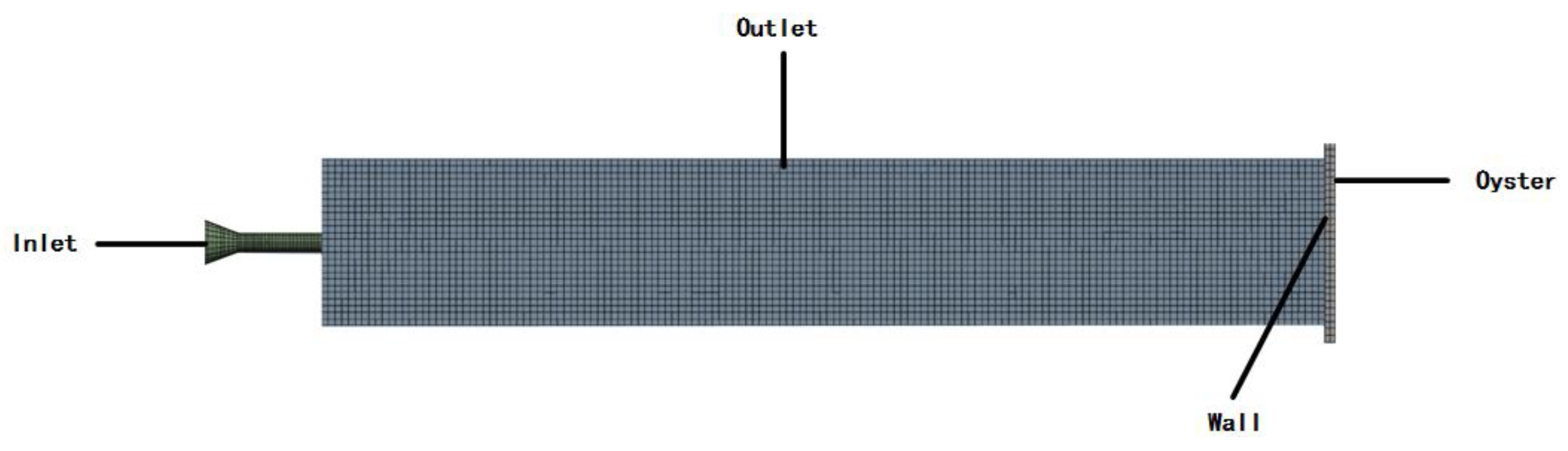
Figure 6.
The process of calculating the comprehensive score of each group of experimental points using the entropy method.
Figure 6.
The process of calculating the comprehensive score of each group of experimental points using the entropy method.
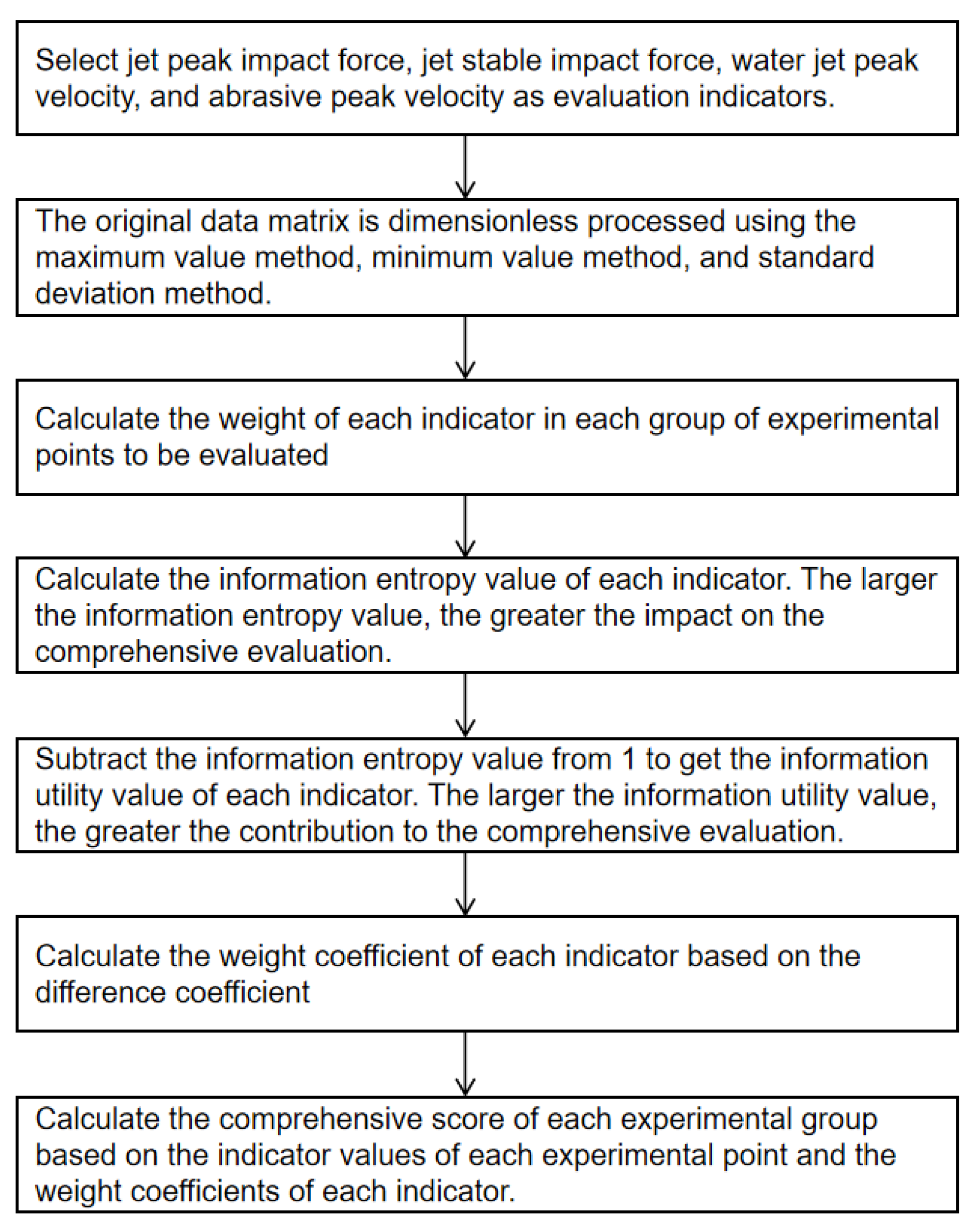
Figure 7.
Predicted values and simulated values.
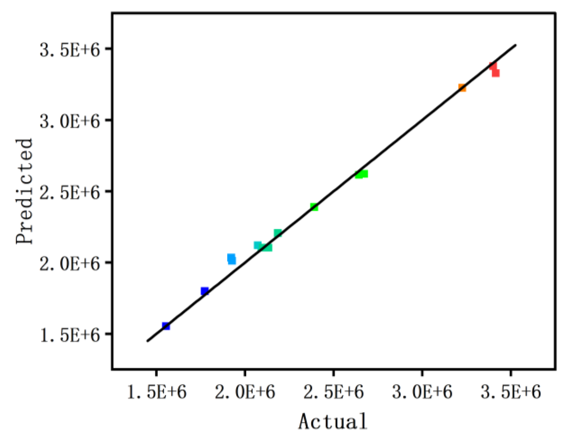
Figure 8.
(a) Relationship between jet’s overall removal capability and nozzle inlet pressure; (b) Relationship between jet’s overall removal capability and outlet diameter; (c) Relationship between jet’s overall removal capability and target distance.
Figure 8.
(a) Relationship between jet’s overall removal capability and nozzle inlet pressure; (b) Relationship between jet’s overall removal capability and outlet diameter; (c) Relationship between jet’s overall removal capability and target distance.
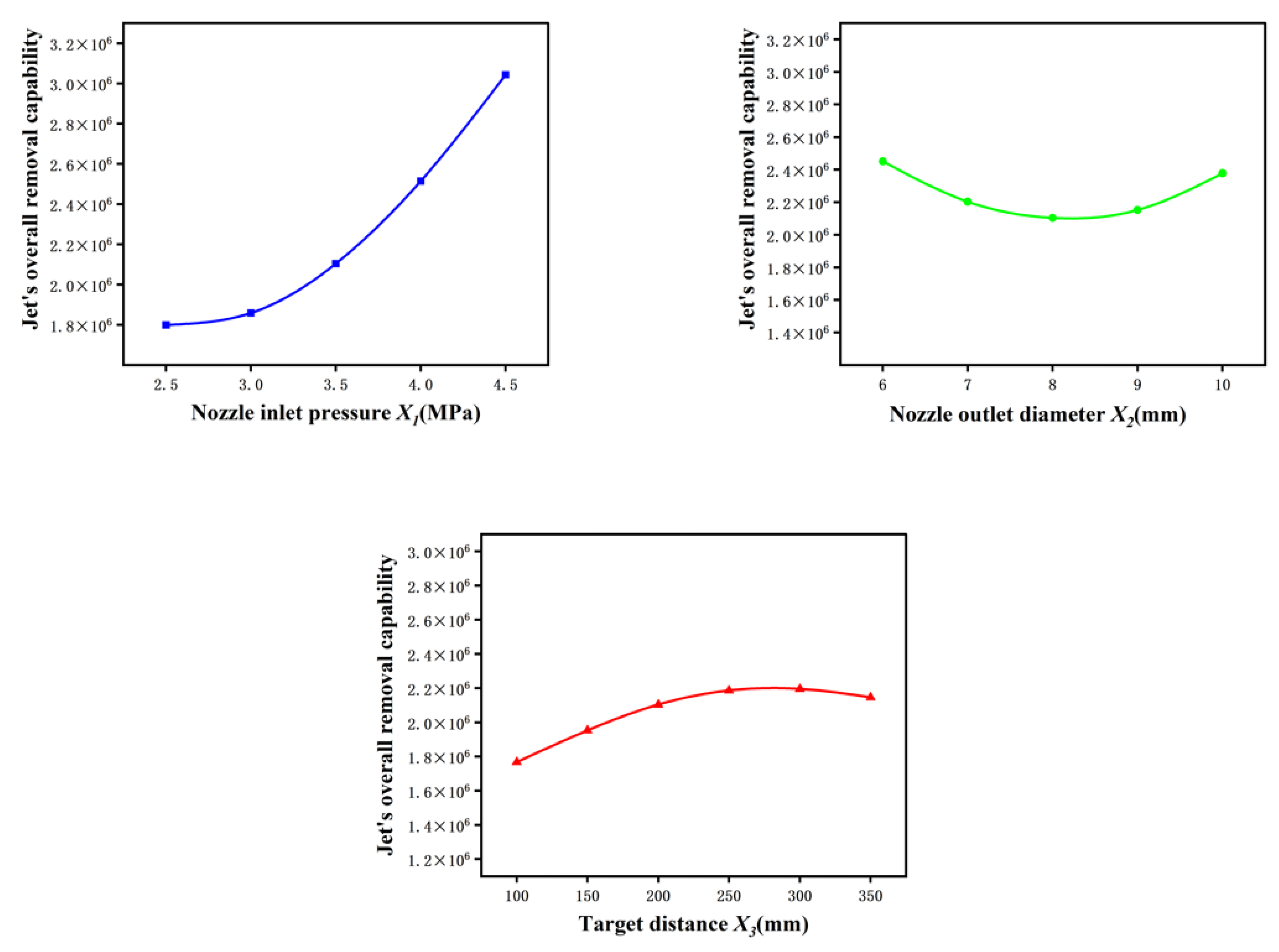
Figure 9.
Effect of the interaction between nozzle inlet pressure and nozzle outlet diameter on the comprehensive stripping ability of the jet(X3 = 200mm).
Figure 9.
Effect of the interaction between nozzle inlet pressure and nozzle outlet diameter on the comprehensive stripping ability of the jet(X3 = 200mm).
Figure 10.
Effect of the interaction between nozzle inlet pressure and target distance on the comprehensive stripping ability of the jet(X2 = 8mm).
Figure 10.
Effect of the interaction between nozzle inlet pressure and target distance on the comprehensive stripping ability of the jet(X2 = 8mm).
Figure 11.
Effect of the interaction between nozzle outlet diameter and target distance on the comprehensive stripping ability of the jet(X1 = 3.5MPa).
Figure 11.
Effect of the interaction between nozzle outlet diameter and target distance on the comprehensive stripping ability of the jet(X1 = 3.5MPa).
Figure 12.
(a) Speed cloud diagram of operating condition 1; (b) Pressure cloud diagram of operating condition 1; (c) Speed cloud diagram of operating condition 2; (d) Pressure cloud diagram of operating condition 2; (e) Speed cloud diagram of operating condition 3; (f) Pressure cloud diagram of operating condition 3.
Figure 13.
(a) The speed distribution of abrasive water jet along the axis under 3 working conditions; (b) The speed distribution of abrasive along the axis under 3 working conditions; (c) The impact force of abrasive water jet under 3 working conditions.
Figure 13.
(a) The speed distribution of abrasive water jet along the axis under 3 working conditions; (b) The speed distribution of abrasive along the axis under 3 working conditions; (c) The impact force of abrasive water jet under 3 working conditions.
Figure 14.
(a) Abrasive trajectory diagram of working conditions 2 when the water jet just contacts the oyster surface; (b) Abrasive trajectory diagram of working conditions 3 when the water jet just contacts the oyster surface.
Figure 14.
(a) Abrasive trajectory diagram of working conditions 2 when the water jet just contacts the oyster surface; (b) Abrasive trajectory diagram of working conditions 3 when the water jet just contacts the oyster surface.
Figure 15.
LPAWJ cleaning test platform.
Figure 16.
Three replicate oyster removal experiments under Condition 1.
Figure 17.
Three replicate oyster removal experiments under Condition 2.
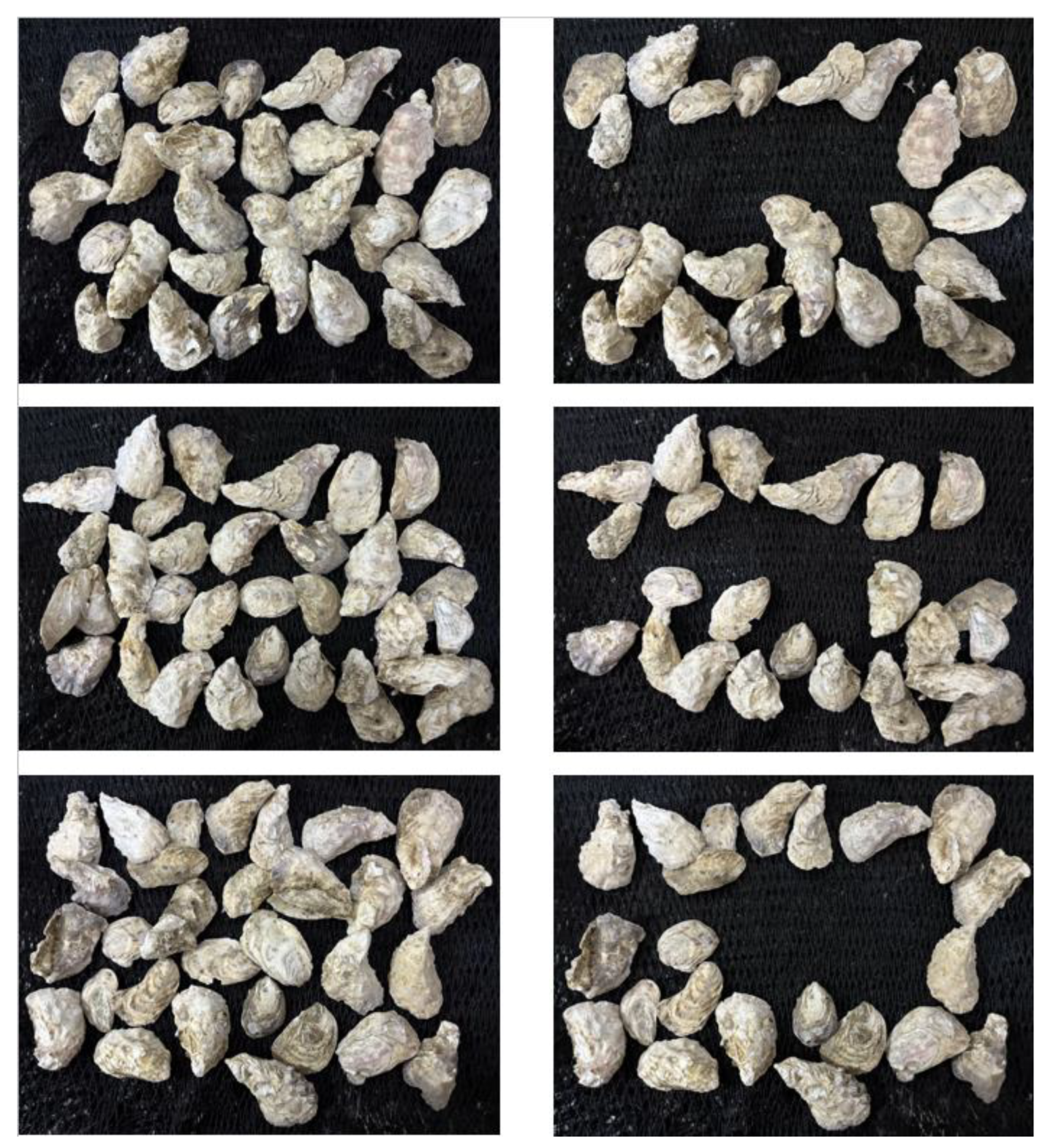
Figure 18.
Three replicate oyster removal experiments under Condition 3.
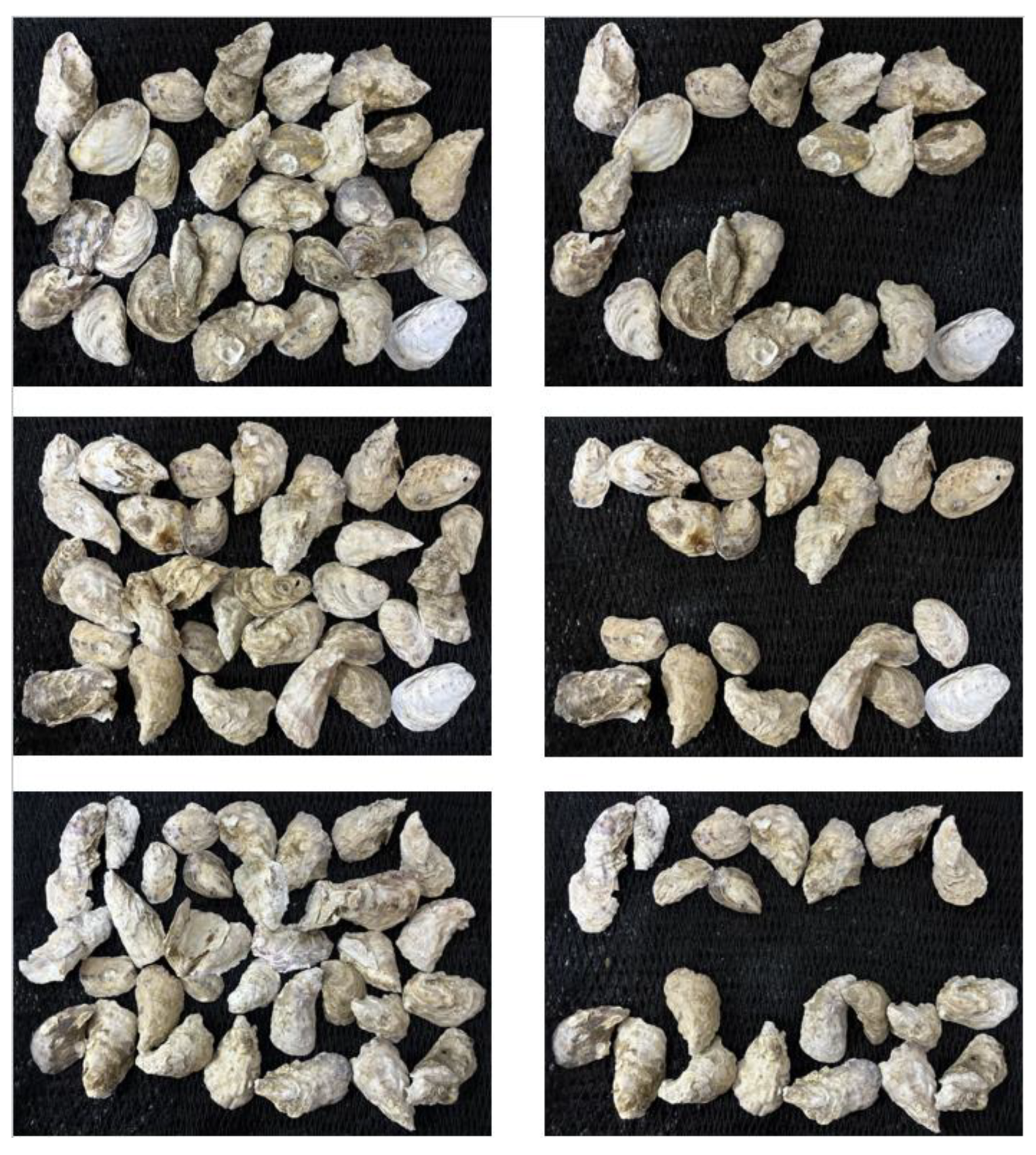

Table 1.
Parameters of quartz sand particles.
| Particle density(kg/m3) | Particle size(mm) | Particle mass flow rate(kg/s) |
|---|---|---|
| 2600 | 0.6 | 0.075 |
Table 2.
Comparison of theoretical and simulated water jet velocities at the nozzle inlet.
| Inlet pressure (MPa) |
Theoretical water jet velocity (m/s) |
Simulated water jet velocity (m/s) |
Error |
|---|---|---|---|
| 2.5 | 70.70 | 70.77 | 0.099% |
| 3.5 | 83.66 | 83.74 | 0.096% |
| 4.5 | 94.86 | 94.95 | 0.095% |
Table 3.
Mesh independence verification.
| Solution | W1 | W2 | W3 | W4 |
|---|---|---|---|---|
| Mesh cell | 15547 | 19413 | 22586 | 27306 |
| Fluid outlet velocity (m/s) | 60.2347 | 76.6049 | 76.5471 | 76.5427 |
| Peak jet impact force (Pa) | 3643625 | 4145702 | 4148243 | 4149645 |
Table 4.
Response surface experiment parameter levels.
| Optimization Parameter | Parameter Code | Unit | Lower Level(-1) | Zero Level(0) | Upper Level(1) |
|---|---|---|---|---|---|
| Nozzle inlet pressure | X1 | MPa | 2.5 | 3.5 | 4.5 |
| Nozzle outlet diameter | X2 | mm | 6 | 8 | 10 |
| Target distance | X3 | mm | 100 | 200 | 300 |
Table 5.
Experimental results.
| Run | X1(MPa) | X2(mm) | X3(mm) | Z1(Pa) | Z2(Pa) | Z3(m/s) | Z4(m/s) | Y |
|---|---|---|---|---|---|---|---|---|
| 1 | 3.5 | 8 | 200 | 3772636 | 2563217 | 83.436 | 83.873 | 2131847 |
| 2 | 3.5 | 8 | 200 | 3807649 | 2421355 | 83.400 | 83.815 | 2092102 |
| 3 | 2.5 | 8 | 300 | 2791840 | 2438962 | 80.937 | 80.836 | 1772445 |
| 4 | 3.5 | 10 | 100 | 3487516 | 2650094 | 83.885 | 82.853 | 2071570 |
| 5 | 4.5 | 6 | 200 | 5034319 | 2574198 | 90.678 | 88.586 | 2622321 |
| 6 | 4.5 | 10 | 200 | 5950920 | 4146674 | 97.620 | 95.164 | 3399931 |
| 7 | 3.5 | 6 | 300 | 4073072 | 3795392 | 105.510 | 78.577 | 2671069 |
| 8 | 3.5 | 8 | 200 | 3810632 | 2436794 | 83.396 | 83.815 | 2098607 |
| 9 | 3.5 | 8 | 200 | 3810632 | 2436794 | 83.396 | 83.815 | 2098607 |
| 10 | 4.5 | 8 | 100 | 4491512 | 3341128 | 93.687 | 91.643 | 2642102 |
| 11 | 3.5 | 6 | 100 | 3659127 | 2079154 | 79.694 | 78.368 | 1921461 |
| 12 | 2.5 | 10 | 200 | 3300805 | 2412436 | 74.987 | 73.879 | 1926242 |
| 13 | 3.5 | 8 | 200 | 3810632 | 2436794 | 83.396 | 83.815 | 2098607 |
| 14 | 3.5 | 10 | 300 | 4281541 | 3139775 | 87.091 | 86.871 | 2502358 |
| 15 | 2.5 | 8 | 100 | 2870546 | 2135317 | 69.499 | 68.141 | 1688578 |
| 16 | 2.5 | 6 | 200 | 3938491 | 2561902 | 94.761 | 84.247 | 2184601 |
| 17 | 4.5 | 8 | 300 | 5158842 | 3993358 | 108. 082 | 107.420 | 3090652 |
Table 6.
Weight coefficients of evaluation index values.
| Item | Information entropy value | Information utility value | Weight coefficient |
|---|---|---|---|
| Z1(Pa) | 0.888 | 0.112 | 32.091 |
| Z2(Pa) | 0.875 | 0.125 | 35.937 |
| Z3(m/s) | 0.94 | 0.06 | 17.145 |
| Z4(m/s) | 0.948 | 0.052 | 14.828 |
Table 7.
ANOVA for regression models.
| Source | Sum of Squares | df | Mean Squares | F-Value | P-Value |
|---|---|---|---|---|---|
| Model | 4.912 × 10¹² | 9 | 5.458 × 10¹¹ | 245.36 | < 0.0001 |
| X1 | 3.439 × 10¹² | 1 | 3.439 × 10¹² | 1545.99 | < 0.0001 |
| X2 | 2.042 × 10¹⁰ | 1 | 2.042 × 10¹⁰ | 9.18 | 0.0191 |
| X3 | 4.371 × 10¹¹ | 1 | 4.371 × 10¹¹ | 196.49 | < 0.0001 |
| X1X2 | 1.487 × 10¹⁰ | 1 | 1.487 × 10¹⁰ | 6.69 | 0.0362 |
| X1X3 | 3.324 × 10¹⁰ | 1 | 3.324 × 10¹⁰ | 14.94 | 0.0062 |
| X2X3 | 4.657 × 10¹⁰ | 1 | 4.657 × 10¹⁰ | 20.94 | 0.0026 |
| X12 | 4.618 × 10¹¹ | 1 | 4.618 × 10¹¹ | 207.61 | < 0.0001 |
| X22 | 3.693 × 10¹¹ | 1 | 3.693 × 10¹¹ | 166.02 | < 0.0001 |
| X32 | 7.868 × 10¹⁰ | 1 | 7.868 × 10¹⁰ | 35.37 | 0.0006 |
| Residual | 1.557 × 10¹⁰ | 7 | 2.224 × 10⁹ | ||
| Lack of Fit | 1.457 × 10¹⁰ | 3 | 4.856 × 10⁹ | ||
| Pure Error | 0 | 4 | 0 | ||
| Cor. Total | 4.928 × 10¹² | 16 |
Table 8.
Evaluation results of the regression model.
| R2 | Adj R2 | Pred R2 | Adeq Precision | C.V |
|---|---|---|---|---|
| 0.9968 | 0.9928 | 0.9524 | 52.447 | 2.02% |
Table 9.
Comparison of simulation results and optimization results under Condition 3.
| Z1(Pa) | Z2(Pa) | Z3(m/s) | Z4(m/s) | Actual Y value | Predicted Y value |
|---|---|---|---|---|---|
| 6313952 | 4029857 | 93.9754 | 93.6029 | 3474450 | 3408646 |
Table 10.
Oyster removal rates under the three operating conditions.
| Condition1 | Condition2 | Condition3 | |||||||
|---|---|---|---|---|---|---|---|---|---|
| Rb(%) | Ra(%) | R(%) | Rb(%) | Ra(%) | R(%) | Rb(%) | Ra(%) | R(%) | |
| Group 1 | 61. 43 | 51. 38 | 16. 35 | 54. 64 | 38. 18 | 30.11 | 61. 95 | 41. 59 | 32. 85 |
| Group 2 | 57. 26 | 47. 94 | 16. 27 | 54. 35 | 38. 01 | 30. 05 | 62. 31 | 42. 14 | 32. 37 |
| Group 3 | 61. 27 | 51. 43 | 16. 06 | 53. 91 | 37. 77 | 29. 93 | 59. 16 | 39. 97 | 32. 44 |
Disclaimer/Publisher’s Note: The statements, opinions and data contained in all publications are solely those of the individual author(s) and contributor(s) and not of MDPI and/or the editor(s). MDPI and/or the editor(s) disclaim responsibility for any injury to people or property resulting from any ideas, methods, instructions or products referred to in the content. |
© 2025 by the authors. Licensee MDPI, Basel, Switzerland. This article is an open access article distributed under the terms and conditions of the Creative Commons Attribution (CC BY) license (http://creativecommons.org/licenses/by/4.0/).
Copyright: This open access article is published under a Creative Commons CC BY 4.0 license, which permit the free download, distribution, and reuse, provided that the author and preprint are cited in any reuse.


