1. Introduction
Cavitation is the transition from the liquid state to the gas state without addition of heat (unlike boiling) because of a pressure decrease, when the pressure falls below a critical value that is approximately equal to the vapor pressure.
Cavitation can be generated in different ways [
1,
2]. (i) The geometry of the system creates velocity variations and consequently pressure variations. This type of cavitation is called hydrodynamic cavitation and it is the most common type in hydraulic machinery and hydraulic systems (ii) The pressure variations are produced by sound waves, usually ultrasound and thus it is called ultrasonic cavitation. (iii) Optical cavitation is produced by a laser that creates bubbles (usually a single bubble).
Cavitation produces the erosion of the surrounding material if the collapses take place close to it. Two main phases can be distinguished in the cavitation erosion process: 1) the incubation period, wherein only small plastic deformations (pits) due to plastic deformation can be seen, and 2) the period with material detachment and separation from the surface which follows the previous one and results in mass loss [
3].
AE is defined as the high frequency vibration induced in a solid material due to elastic waves traveling inside it [
4]. The elastic waves are the result of the energy released in the material due to sudden changes in the internal stresses, external impacts or surface contacts. As an AE source, cavitation represents external impacts resulting from bubble collapses near of a solid boundary [
5]. AE has a wide frequency band, but low frequencies below 100 kHz are usually removed to filter out unwanted noise [
5,
6]. AE has been used to detect cavitation and to study it as for example describe in the work of Escaler et al. [
7] who detected cavitation in several turbines using AE and other quantities (like vibrations and dynamic pressures). Signals were demodulated and different characteristic frequencies were identified. Another researcher, Ylönen [
8], studied erosion in cavitation tunnel using AE. The works presented in [
9] and [
10] studied the incubation period and a relationship between the cumulative distribution between the amplitude peak values and pit diameters was established. As shown in [
5], it was concluded than the shedding frequency obtained by demodulating the AE increases when erosion depth increases. Finally, a comprehensive review of the use of AE to detect and analyze cavitation was presented in [
11].
Different researchers have studied the relationship between the temperature of the liquid in which cavitation occurs and the erosion produced. Hattori et al. [
12] submitted specimens of pure copper and pure aluminium to cavitating liquid jet tests at different temperatures and they measured the mass loss. They concluded that mass loss increases as the temperature of the liquid increases until it reaches a maximum, followed by a decrease. Li et al. [
13] submitted stainless steel (AISI 304) specimens to ultrasonic cavitation at different temperatures that ranged between 20° and 80°and they measured the mass loss. They found the maximum mass loss in the range between 45° to 50°. Priyadarshi et al. [
14] submitted two kinds of cast aluminium specimens (A356.2 and A380) to ultrasonic cavitation at different temperatures that ranged from 10° to 50°, and they measured the mass loss. They found the maximum mass loss at 30°. Dular [
15] submitted aluminium specimens to cavitation in a cavitation tunnel at different temperatures that ranged from 30° to 100°. The erosion was evaluated in the incubation period by pit counting. The maximum erosion (maximum number of pits) was found at 60°.
The relationship between the roughness of the surface submitted to cavitation has been also studied. Escaler et al. [
16] found out that the cavitation aggressiveness was greater the larger the roughness of the tested specimen with a roughly linear relationship. Hao et al. [
17] studied the influence of the rugosity on the cloud cavitation behaviour. They concluded that the cavity on the rough surface could break off, shed, and collapse more than one time in a period, which could lead to more severe cavitation erosion.
In this paper, the influence of fluid temperature and material surface condition on the number and intensity of cavitation impacts has been experimentally studied. A series of measurements of cavitation-induced AEs have been carried out in a closed loop cavitation tunnel with a Venturi test section and a metallic sample. The sample has been submitted to cloud cavitation for a very long period of time to observe at simple sight cavitation damage. An AE-based parameter has been defined to evaluate cavitation impacts and to quantify the effects on cavitation aggressiveness. More specifically,
Section 2 describes the test bench, the performed tests, and the definition of the AE parameter to estimate cavitation impacts.
Section 3 presents the obtained results corresponding to operating parameters, cavitation aggressiveness levels and observed cavitation erosion. And finally,
Section 4 presents a discussion of the results and the main conclusions.
2. Materials and Methods
2.1. Test Bench Description
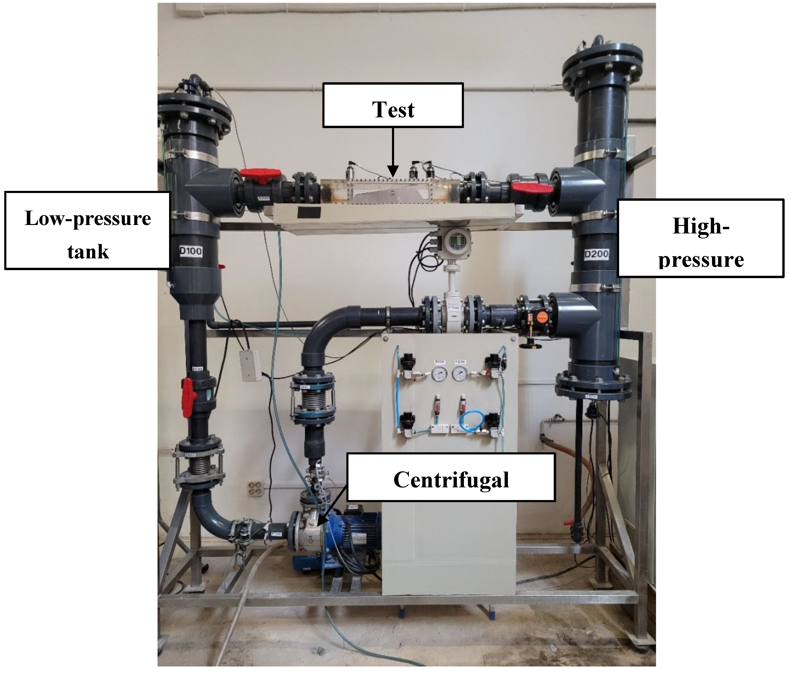
Tests were performed in a cavitation tunnel at the Barcelona Fluids & Energy Lab (IFLUIDS). The cavitation tunnel consists of a closed loop circuit made in PVC pipes (
Figure 1). Circulation of water is obtained with a 3-kW centrifugal pump whose rotating speed is controlled with a variable frequency drive. At the pump delivery a partially filled tank (high pressure tank) is used for damping the pressure fluctuations induced by the pump. Cavitation and its effects can be observed in a transparent PMMA test section where a Venturi has been placed to produce a static pressure drop at the throat and cause the corresponding cavitation (
Figure 2). After the test section there is another partially filled tank (low pressure tank) and finally the water returns to the pump.
The system is instrumented with several sensors to measure the hydraulic variables: 1) absolute pressure sensors at the pump inlet, pump outlet, high pressure-tank, low pressure tank, Venturi inlet, Venturi throat and Venturi outlet; 2) temperature sensors at the bottom of the high-pressure tank and at the top of the low-pressure tank; 3) a magnetic flowmeter; and 4) a pump’s variable frequency drive (VFD) to control the pump rotating speed. A more detailed description of the cavitation tunnel is presented in [
18].
The pressures at free surfaces of the high- and low-pressure tanks at the inlet and outlet of the Venturi, respectively, can be controlled through a pneumatic system feed with compressed air which can increase or reduce the pressures at will.
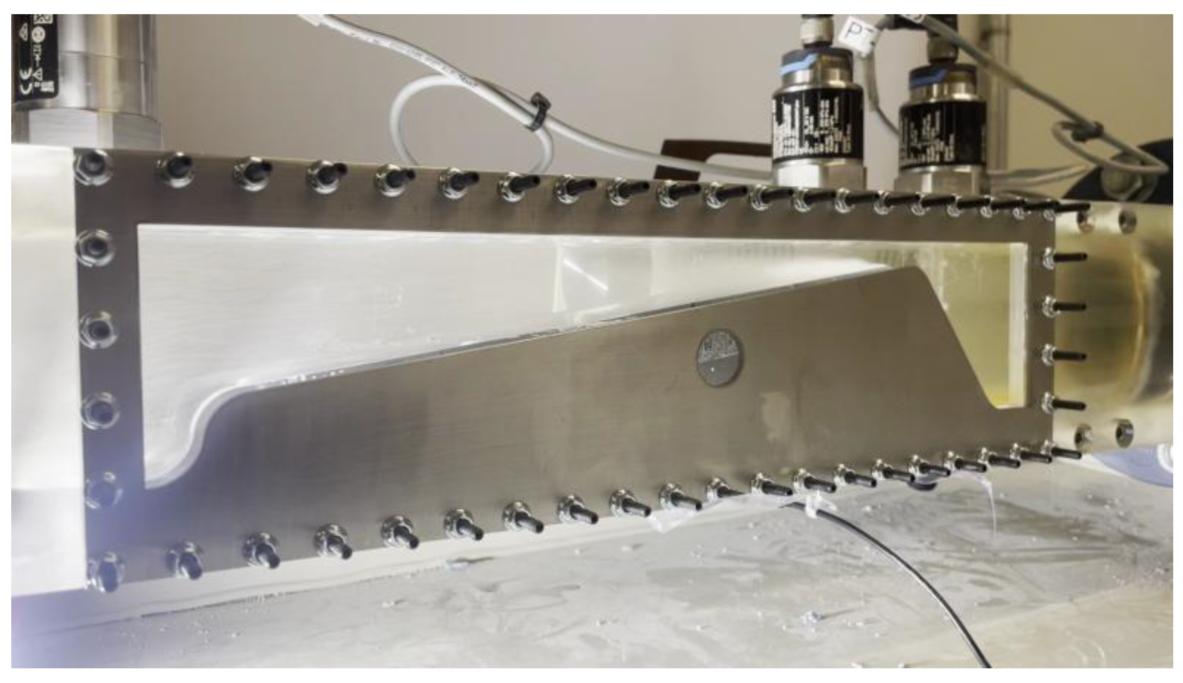
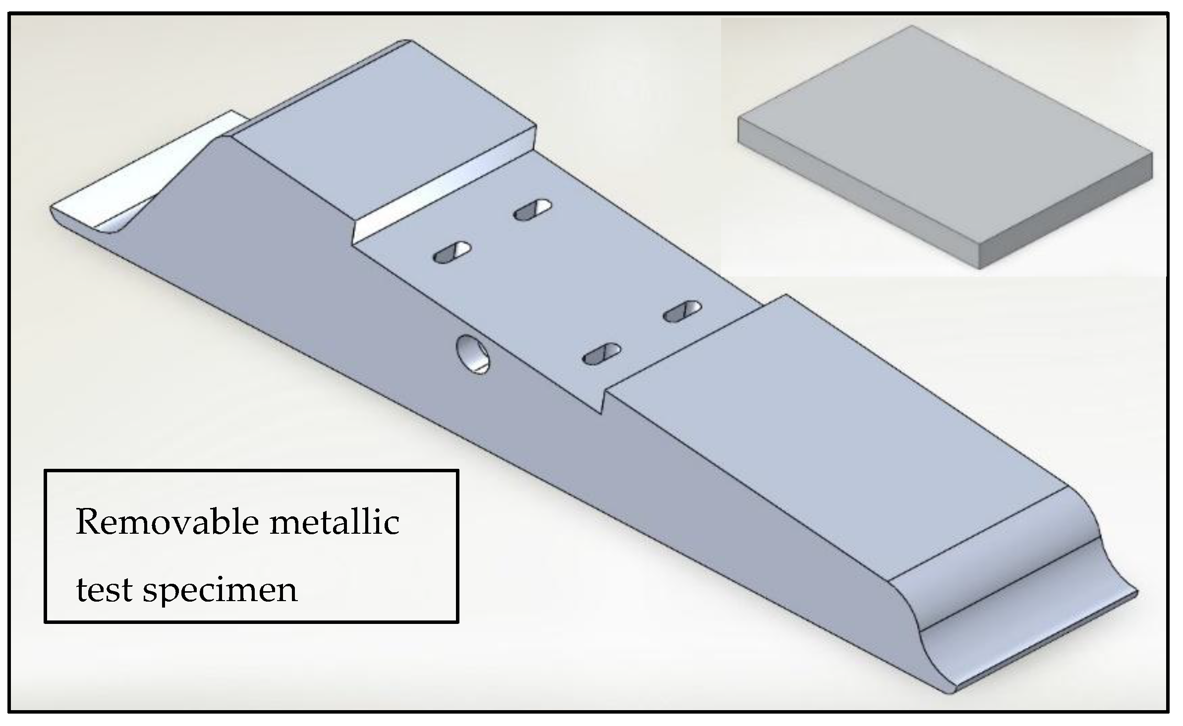
The basic geometry of the test section is a squared 72-millimeter-wide Venturi section consisting of a converging zone, followed by a throat section of 10 x 72 millimetres, and a diverging zone with an angle of 8°. The divergent zone has a housing to place the specimen as shown in
Figure 3. The throat presents a slight groove for triggering a homogeneous cavitation inception in spanwise direction. This particular geometry was designed to be effective in creating cloud cavitation with significant erosive power along the material specimens after evaluating different dimensions and shapes using numerical simulations and experiments.
2.2. Test Description
A 7075-T6 aluminum specimen was manufactured and mounted on the Venturi installed in the test section (
Figure 3). This particular material is difficult to erode due to its high strength and hardness. Its mechanical properties are a yield strength of 503 MPa, an ultimate tensile strength of 572 MPa and a Brinell hardness of 150 [
19].
A long duration erosion test was carried out for 50 hours at steady flow conditions with periodic shedding cloud cavitation. The total running time was divided in 2-hour periods in order to avoid an excessive temperature increase induced by the heating of the pump. At the beginning of each period the water was always at ambient temperature. Pressures and flow rate were maintained stable and similar for all the runs in order to achieve cloud cavitation conditions with a constant maximum length in the range between 70 and 110 mm, so the cavitation attack and the erosion always occurred within the aluminum specimen at the same location.
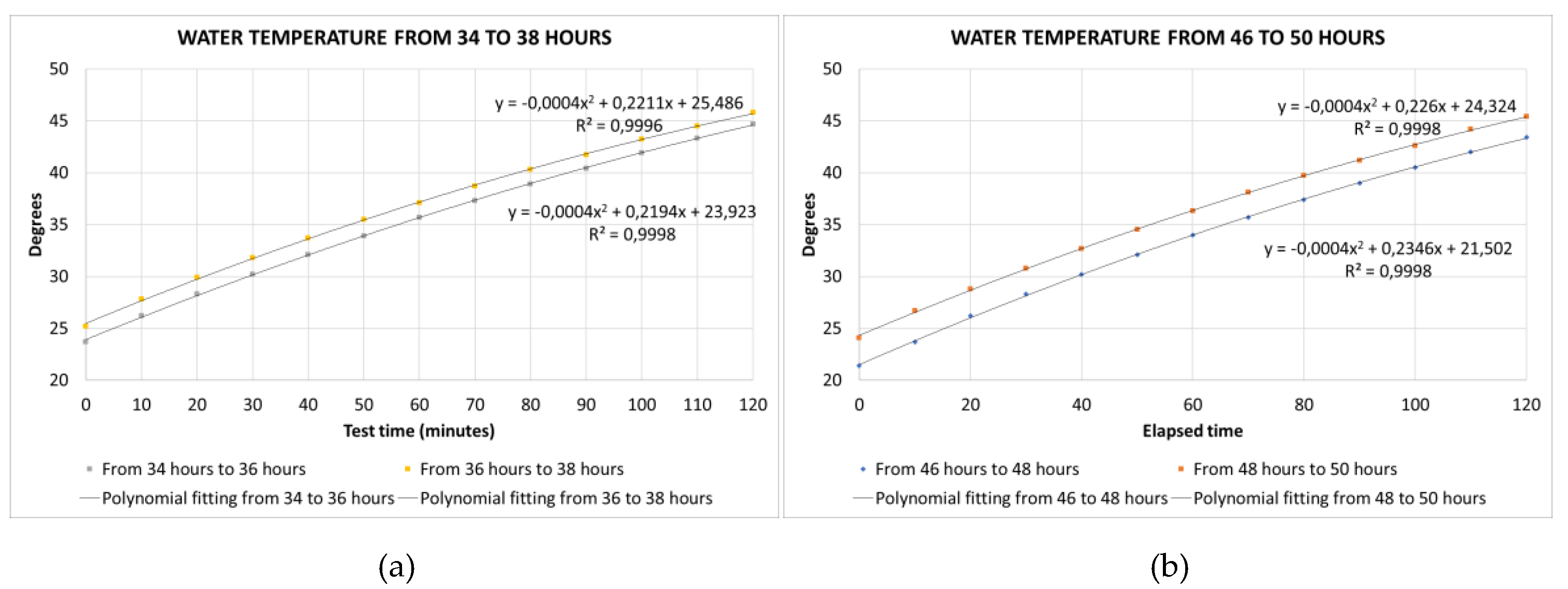
It is important to clarify that during a 2-hours period test, the temperature of the system always increases around 20° as it can be seen in the plots in
Figure 4 where the temperature evolution is presented as a function of time. This temperature increase provokes an increase of the system pressure due to the heating of the air masses above the free surfaces on the upper part of the two tanks. Consequently, a reduction of the maximum length of the cloud cavitation can be observed which needs to be corrected to keep similar aggressiveness levels and erosion location. Therefore, and in order to keep the sheet length in the range between 70 mm and 110 mm, successive purges of the air contained in upper part of the high-pressure tank have to be carried out during each 2-hours test.
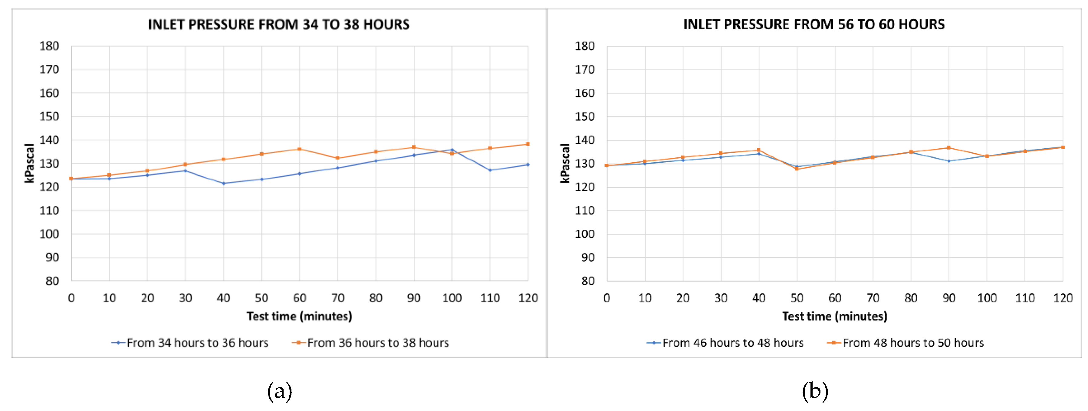
Figure 5 shows the evolution of the pressure at the Venturi inlet where the pressure drops occur during the purging process as air is released from the tank and the pressure is reduced. Between these drops, the pressure increases steadily because the temperature increases as explained before. As this correction is done manually during the tests by the tunnel operator, some differences between different runs can be observed as this process has not been automatized yet.
Two specifics time intervals of 4-hours, comprising two consecutive tests of 2-hours each, were chosen at the middle and at the end of the erosion tests. More precisely, these two periods were from 34 to 38 hours and from 46 to 50 hours, respectively. During them, AE measurements were periodically recorded each 10 minutes and photographs of the sample surface at their end were taken to assess the evolution of the erosion. The first-time interval only showed an initial erosion stage, but the second one already presented a significant amount of erosion on the sample which was not concentrated but dispersed (see Figures 14–16).
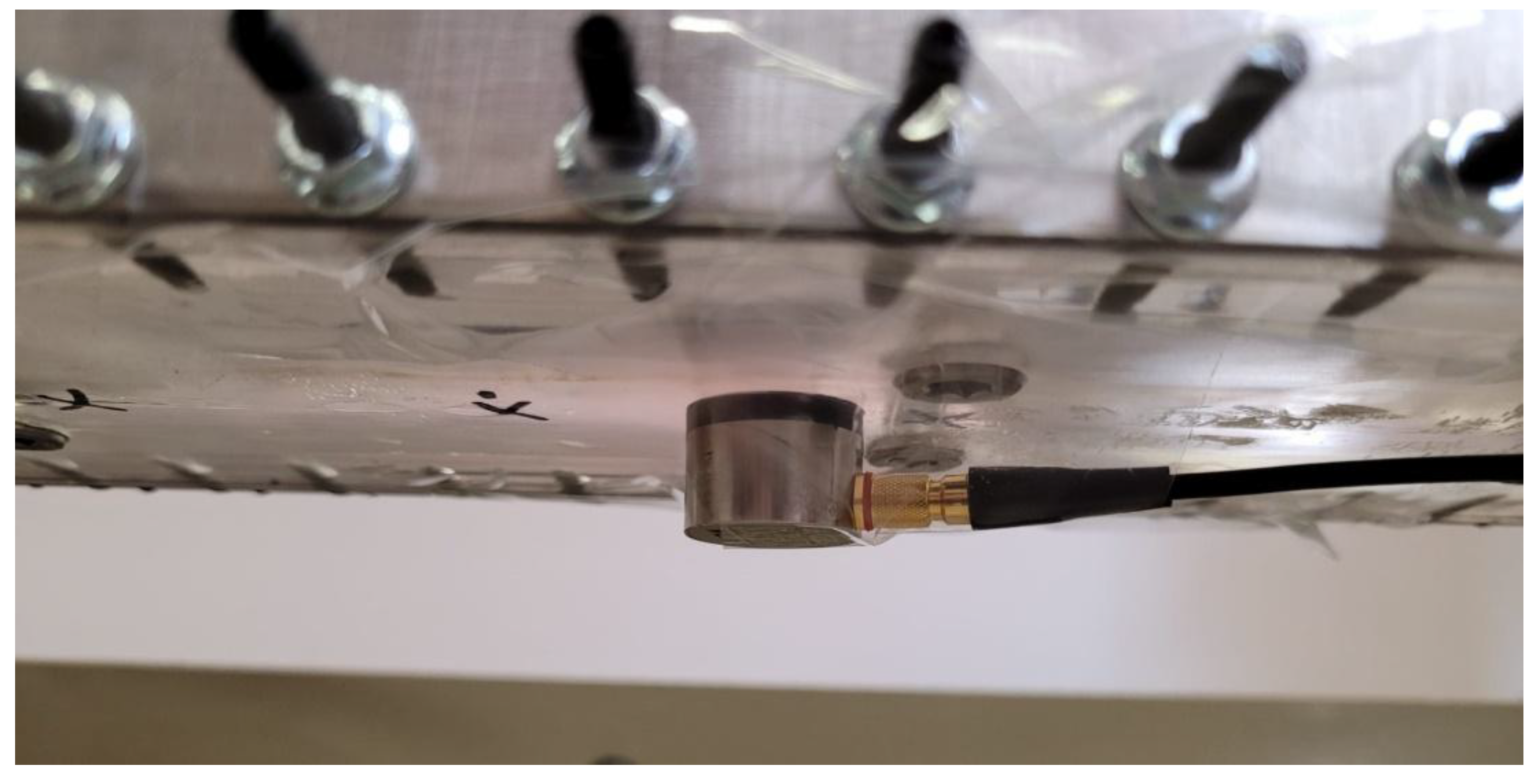
In order to measure the AE caused by the cavitation, a sensor Vallen model 150-M was fitted at the bottom of the test section as shown in
Figure 6. The rest of the AE setup is a Vallen preamplifier AEP5, a Vallen decoupling box DCPL2, and a National Instruments cDAQ 9185 that was connected to a laptop via Ethernet cable. The sampling rate was 20 kHz and the measurement duration of the records was 20 seconds. This means that each measurement consisted of 20 million samples.
2.3. Envelope Extraction of Acoustic Emissions
In order to determine the cavitation dynamic behavior from the AE induced by the cavitation attack on the aluminum sample, it is considered that each collapse of a shed cloud results in a high-pressure short duration pulse on the sample surface that excites the solid like a hammer hitting in a small area. Therefore, the AE transmitted through the Venturi and measured by the sensor on the external bottom wall of the test section appears to be modulated in amplitude at the particular shedding frequency of cloud cavitation. Then this shedding frequency can be inferred from the measured AE applying an amplitude demodulation signal processing method to its time signal.
The amplitude demodulation procedure is based on the Hilbert transform. The Hilbert transform of a real-valued time-domain signal
is another real-valued time-domain signal
, which combined in the following way
provide the so-called analytic signal
. The magnitude function of the analytic signal,
, describes the envelope of the original function
[
20].
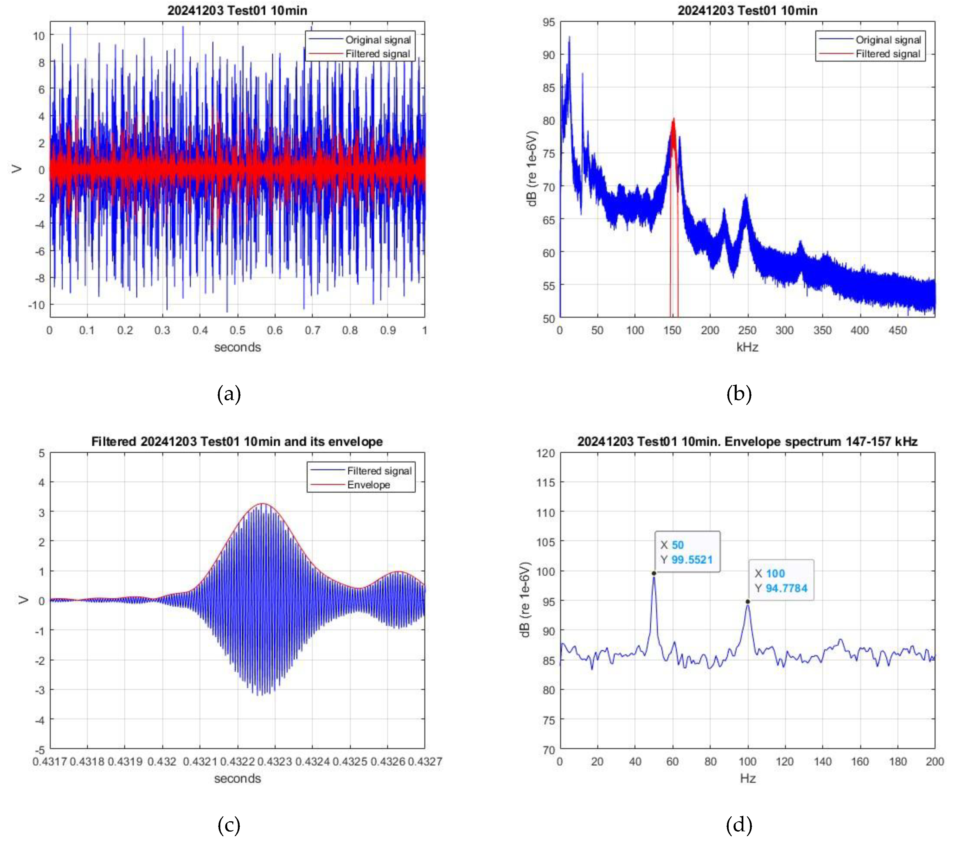
The Hilbert transform demodulation procedure requires a narrowband signal. Then the first step in this analysis is a bandpass filtering to obtain a signal to which the Hilbert procedure can be applied. The filtered signal is also modulated, as can be seen in
Figure 7(a), and it is a narrow band signal as it can be seen in
Figure 7(b) which allows the Hilbert demodulation procedure to be applied. To increase the accuracy of the method, a high signal level is required to apply the band pass filter. In our particular case, the frequency band from 147 to 157 kHz has been selected because it contains the first sensor resonance frequency (
Figure 7(b)) and it has a good signal-noise ratio. Finally, the envelope of the filtered signal is calculated with the Hilbert transform method as shown in
Figure 7(c). And finally, the spectrum of this envelope is calculated using the Fast Fourier Transform to determine the exact value of the amplitude modulation induced by the periodic collapse of the cloud cavitation as it can be seen in
Figure 7(d) with a peak frequency around 50 Hz and its second harmonic around 100 Hz.
2.4. Cavitation Power Indicator Definion
In order to estimate the aggressiveness of cavitation, a power parameter has been de-fined according to the procedure explained as follows:
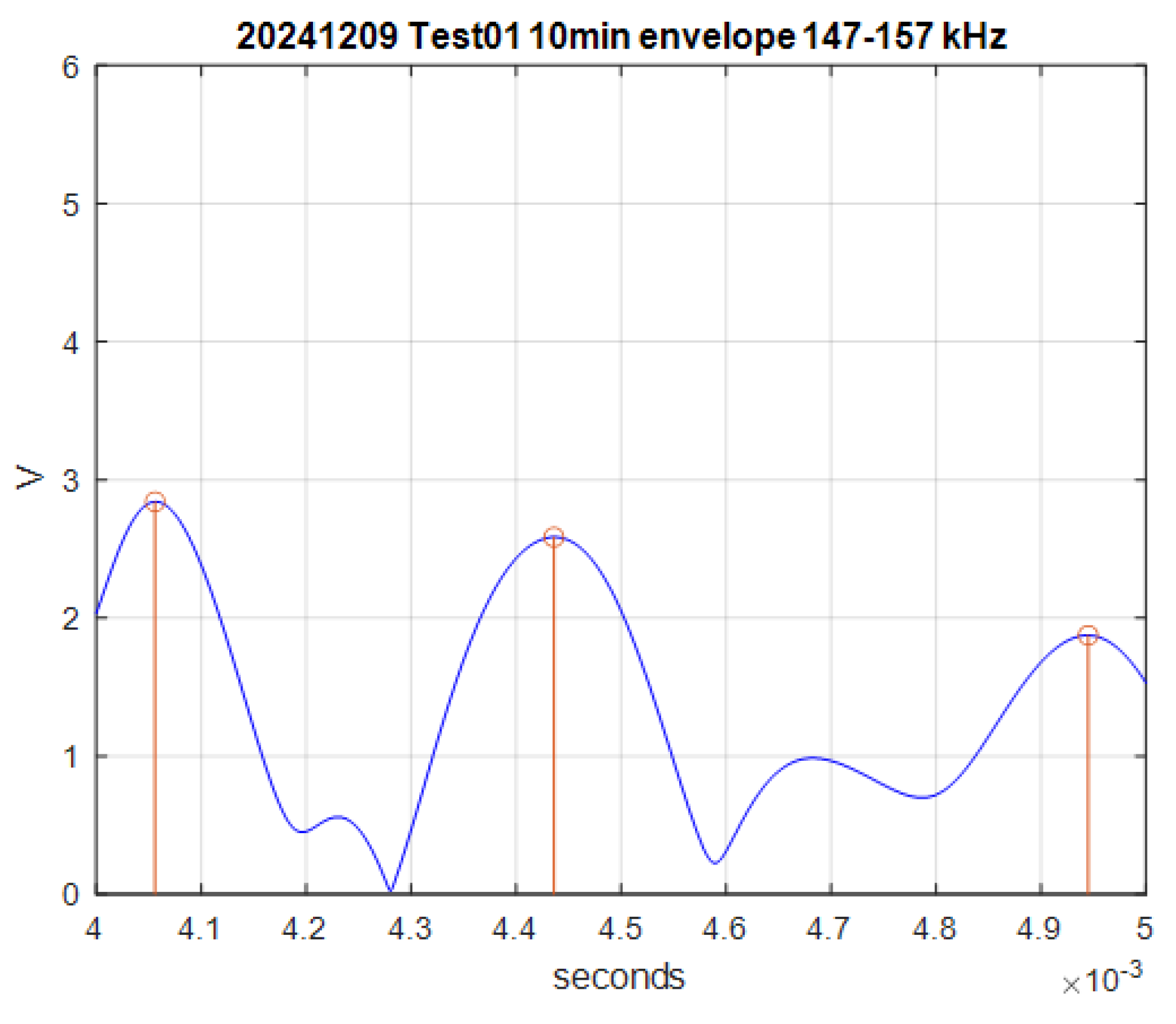
The peak values
of the envelope function, calculated following the procedure described in the previous
Section 2.3, with amplitudes higher than 1 V are counted. In
Figure 8 three of these peaks are identified in a short period of time of 1 millisecond.
The total number of the peak values are grouped in 6 clusters corresponding to increasing ranges of amplitudes: , , , , , and
Then an energy parameter,
, is defined considering all the clusters:
where
is the number of elements of the cluster
.
Finally,
is divided by the duration of the AE signal (20 seconds) to obtain a power indicator,
, that does not depend on the duration of the measured AE signal and whose units are
:
3. Results
First, the evolution of the test rig operating parameters during the tests are presented. These parameters are the temperatures, pressures, cloud cavitation shedding frequencies and cavitation numbers calculated according to the following expression:
where
is the static pressure at the outlet of the test section,
is the water vapor pressure,
is the water density, and
is the water speed at the throat.
Then, the aluminum surface condition and the identified increase of damage between them are also presented. Finally, the cavitation power indicator results are compared between the two different periods.
3.1. Evolution of Operating Parameters During the Tests
Figure 4 shows the temperatures measured at the high-pressure tank and their corresponding fitted curves. The maximum difference between the temperatures of both tanks is 0.1°. Then it can be assumed that the temperature along the cavitation zone is uniform. The temperature evolution shows an increase following a parabolic trend with downward pointing branches as seen in the equations of the fitted curves presented in
Figure 4. The plots are roughly parallel since the differences between the quadratic and linear coefficients of the different fitted parabolas are negligible (see
Figure 4). That is, the temperature evolution throughout the test depends only on its initial value.
Table 1 shows the initial and final temperatures of the tests. The temperature increases are very similar, between 20.6° and 22.0°, and their average is 21.2°.
The pressures at the inlet and outlet of the test section are shown in
Figure 5 and
Figure 9, respectively. At the beginning of each test, it can be observed the pressures increase with the increase of temperature due to the fact that the air mass on the two free-surfaces of the tanks is constant. As previously explained in
Section 2.2, periodic purges of the air contained in upper part of the high-pressure tank are manually carried out to compensate this pressure increase and to keep the pressures roughly constant.
Table 2 shows the maximum and minimum values of inlet and outlet test section pressures and their drop (inlet minus outlet pressures), corresponding to the four analyzed tests. For the intermediate tests, the inlet test section pressures fluctuate between 121.5 and 138.2 kPa, the outlet test section pressures fluctuate between 63.4 and 90.4 kPa; for the final tests, the inlet test section pressures fluctuate between 127.7 and 137.1 kPa, the outlet test section pressures fluctuate between 73.9 and 88.4 kPa. For all the tests, the average range of the test section inlet pressures is 11.7 kPa, and the average range of the test section outlet pressures is 17.9 kPa.
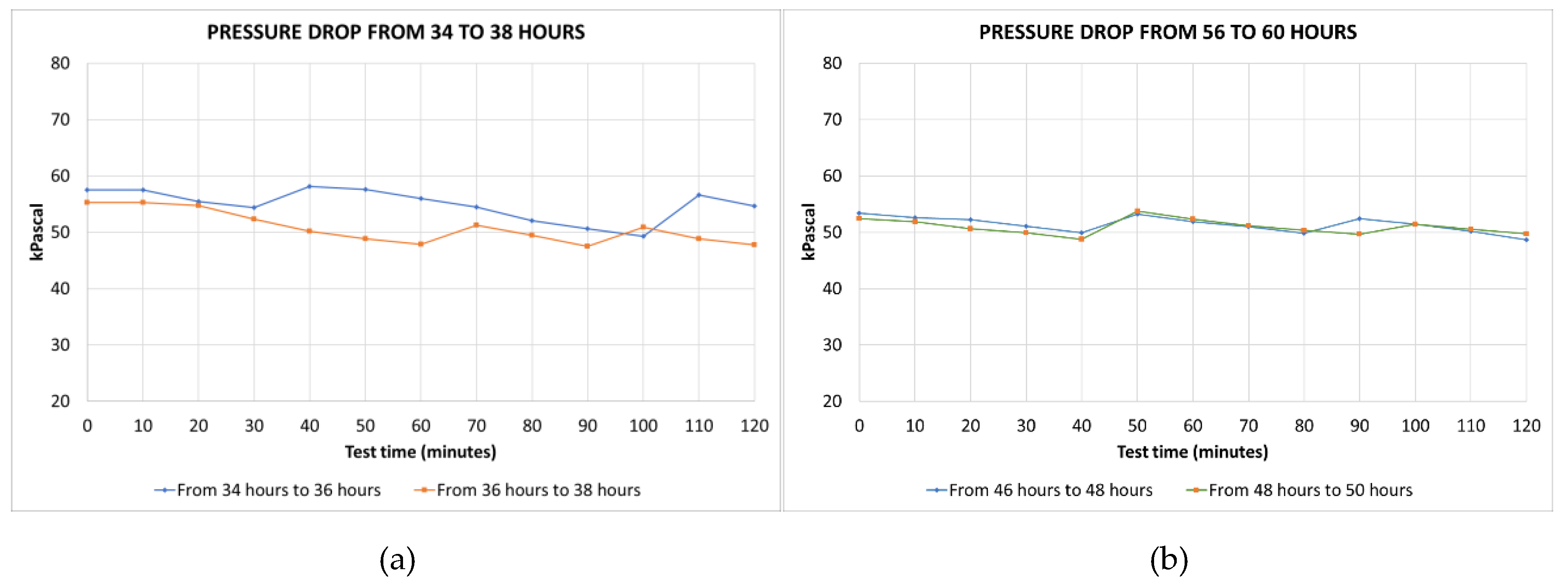
Figure 10 shows the evolution of the pressure drop in the test section (inlet pressure minus outlet pressure). The already commented fluctuations of the inlet and outlet test section pressures are clearly reflected in the pressure drop. But this has the peculiarity that it behaves in an inverse manner: when the inlet and outlet pressures show a maximum, the drop presents a minimum, and when the inlet and outlet pressures show a minimum, the drop presents a maximum. According to
Table 2, for the intermediate tests, the pressure drop fluctuates between 47.5 and 58.1 kPa, and for the final tests, the pressure drop fluctuates between 48.7 and 53.7 kPa. For all tests, the average range of the pressure drop is 6.6 kPa.
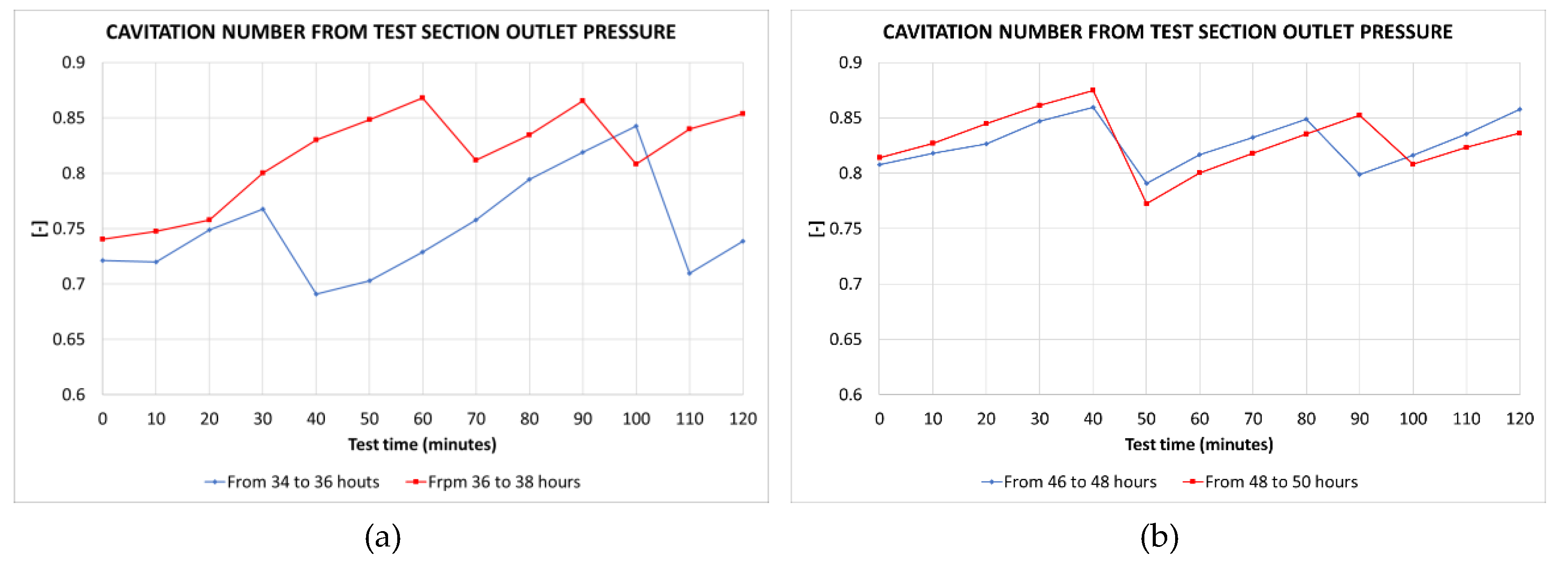
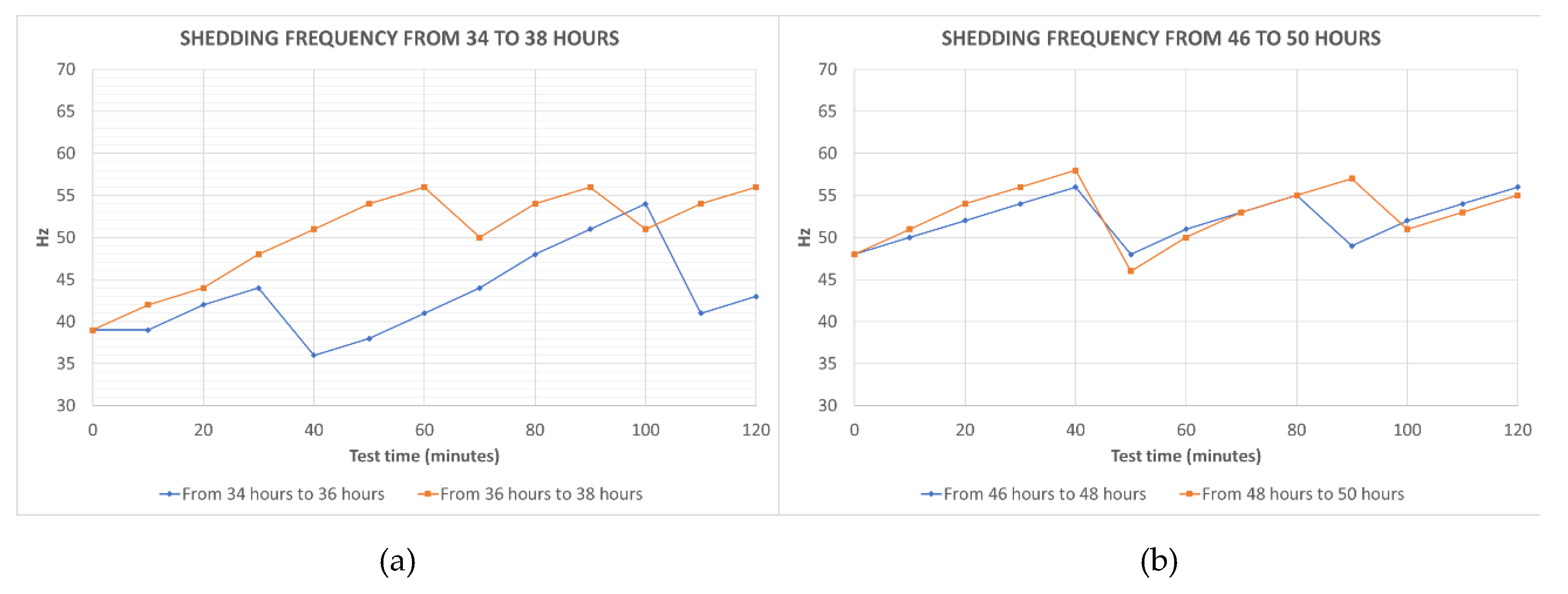
Figure 11 shows the evolution of the cavitation numbers and
Figure 12 shows the evolution of the cloud cavitation shedding frequencies identified from the frequency with a maximum amplitude in the spectrum of the envelope, as explained in
Section 2.3. The fluctuations of the inlet and outlet test section pressures are reflected in the cavitation number and in the shedding frequency values.
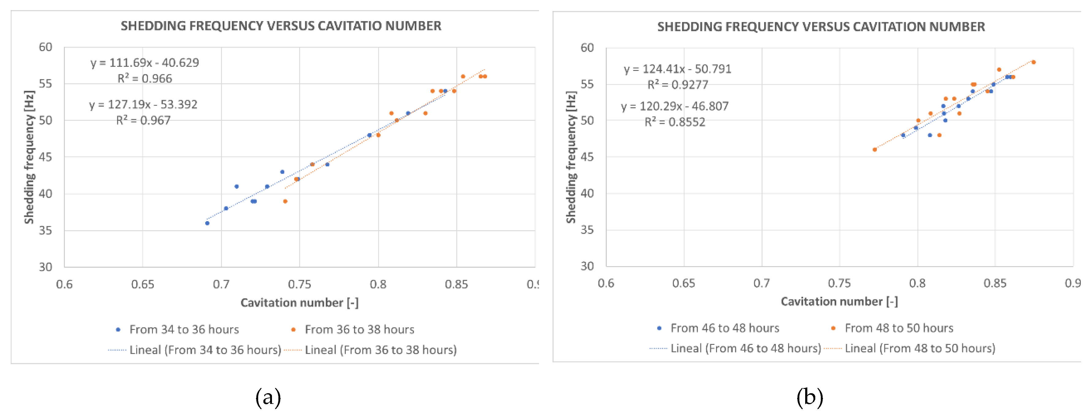
Figure 13 shows the shedding frequency versus cavitation number where a linear relationship between both quantities is noticeable which is roughly the same for the four analyzed tests as seen in the equations of the fitted straight lines presented in
Figure 13.
Then, by averaging the coefficients of the linear equations, the relationship between the cavitation number and the shedding frequency can be estimated with the following expression.
where
is the shedding frequency and
is the cavitation number according to Equation (3).
These results indicate that, when temperature increases then the test section inlet and outlet pressures also increase. Consequently, the cavitation number increases and the maximum length of the cavitation cloud decreases resulting in an increase of the shedding frequency, as it has also been confirmed by visual inspections during the tests. This behavior confirms the necessity to purge the air periodically to maintain the sheet length at an acceptable level.
3.2. Cavitation Erosion Results
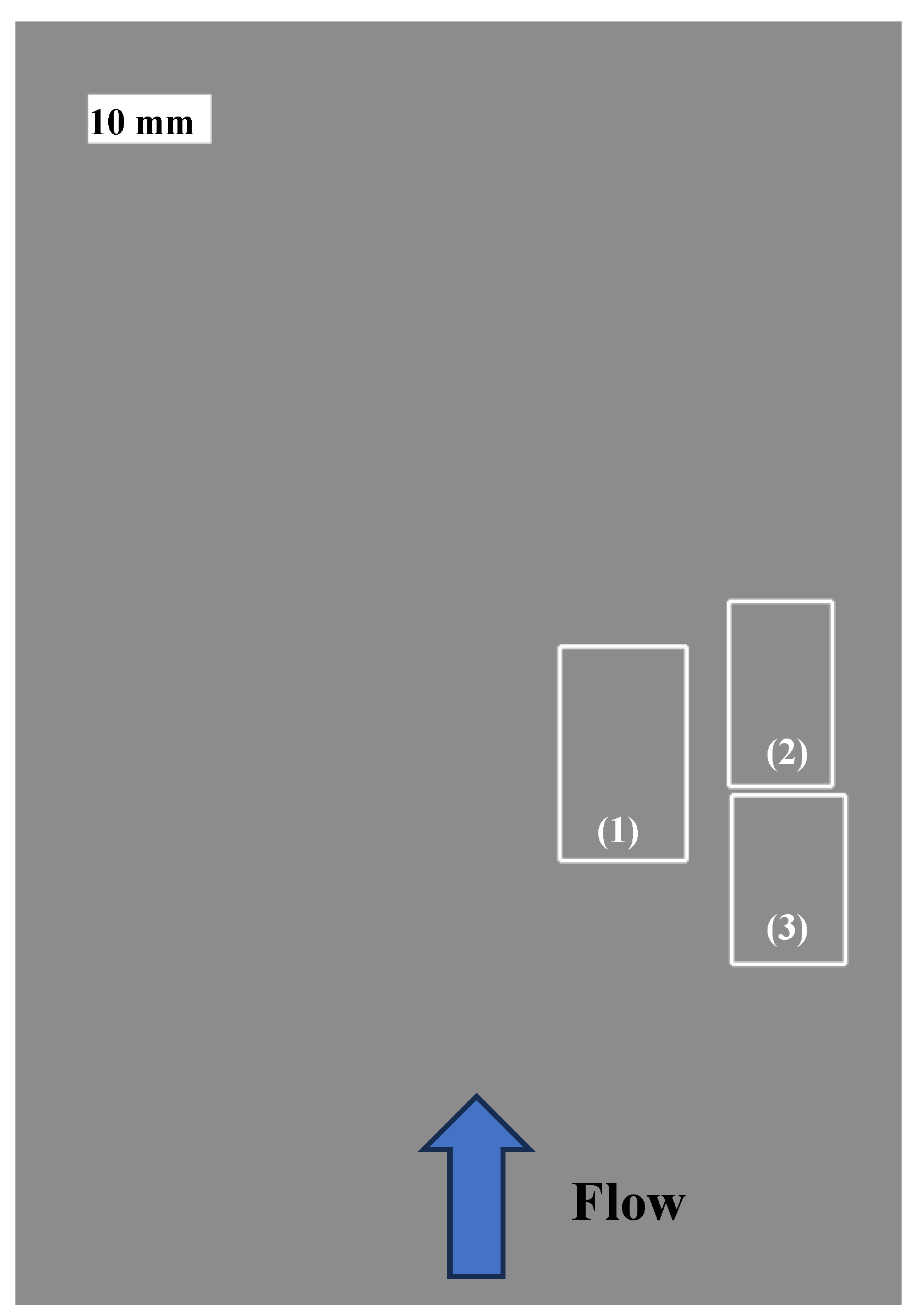
Although the specimen has been submitted to 50 hours of erosive cloud cavitation, damage has not reached yet a measurable mass loss due to the large size and mass of the specimen. In addition, and as explained before, aluminum 7075-T6 is a difficult to erode material because of its high strength and hardness. Then the specimen has not yet been uniformly damaged and not enough damage has accumulated to reach the material removal stage at macroscopic scale. For this reason, three significantly damaged areas with high concentration of pits were selected to analyze the changes in surface condition between the two analyzed periods of time. These areas have been selected because differences between both analysed periods have been observed. The sketch in
Figure 14 shows the position of these selected areas.
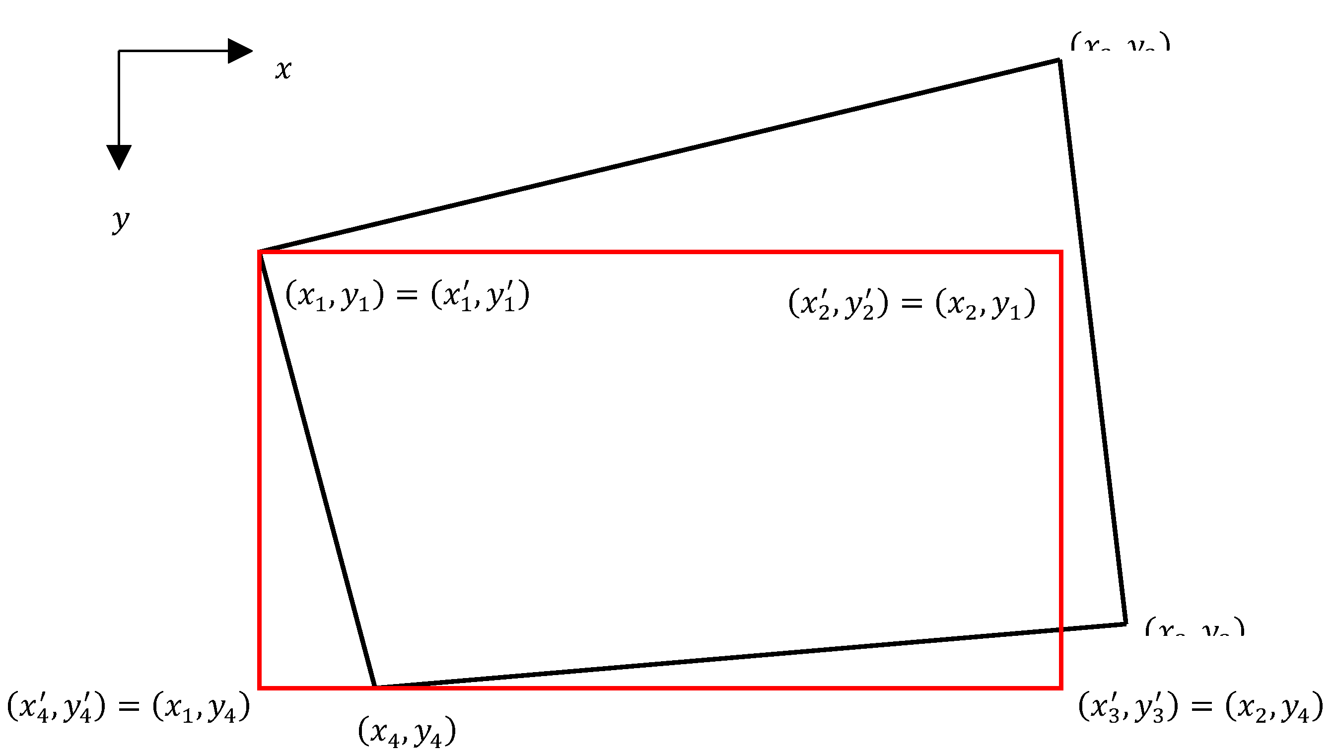
To be able to compare the digital photographs pixel by pixel, given that they were taken from slightly different views, the following procedure was performed in Matlab®:
Projective transformation using the function "tform" that applies the following transformation to the sample vertices with the coordinates shown in
Figure 15.
where
and
are the vertices of the specimen, and
,
,
and
are the vertices of the transformed specimen.
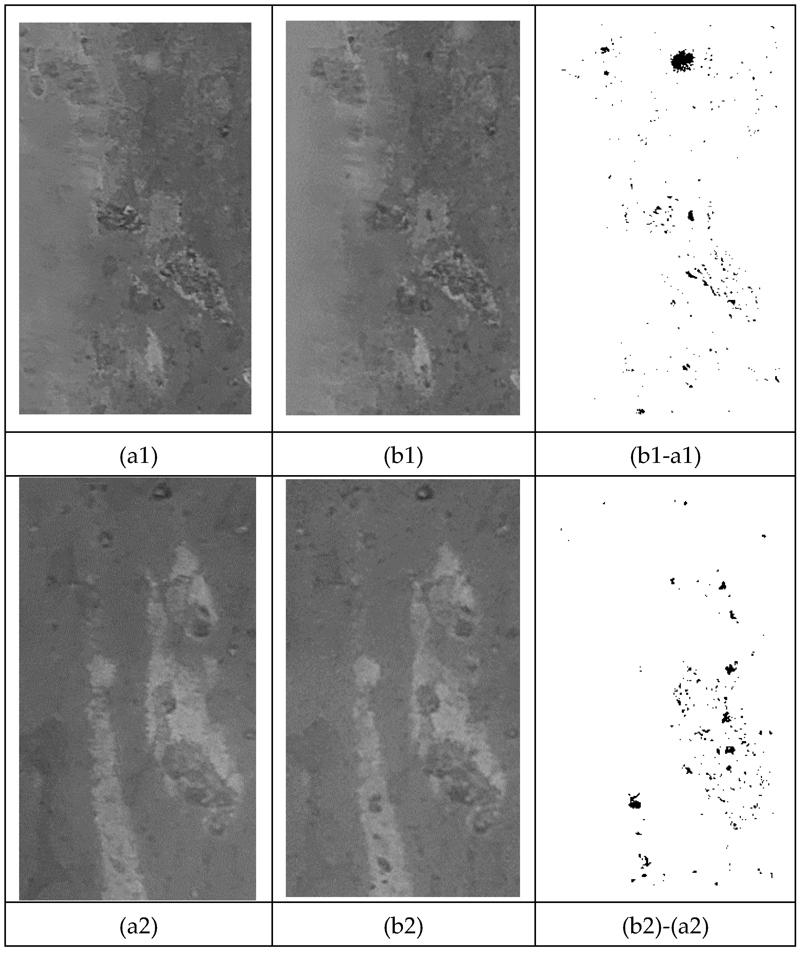
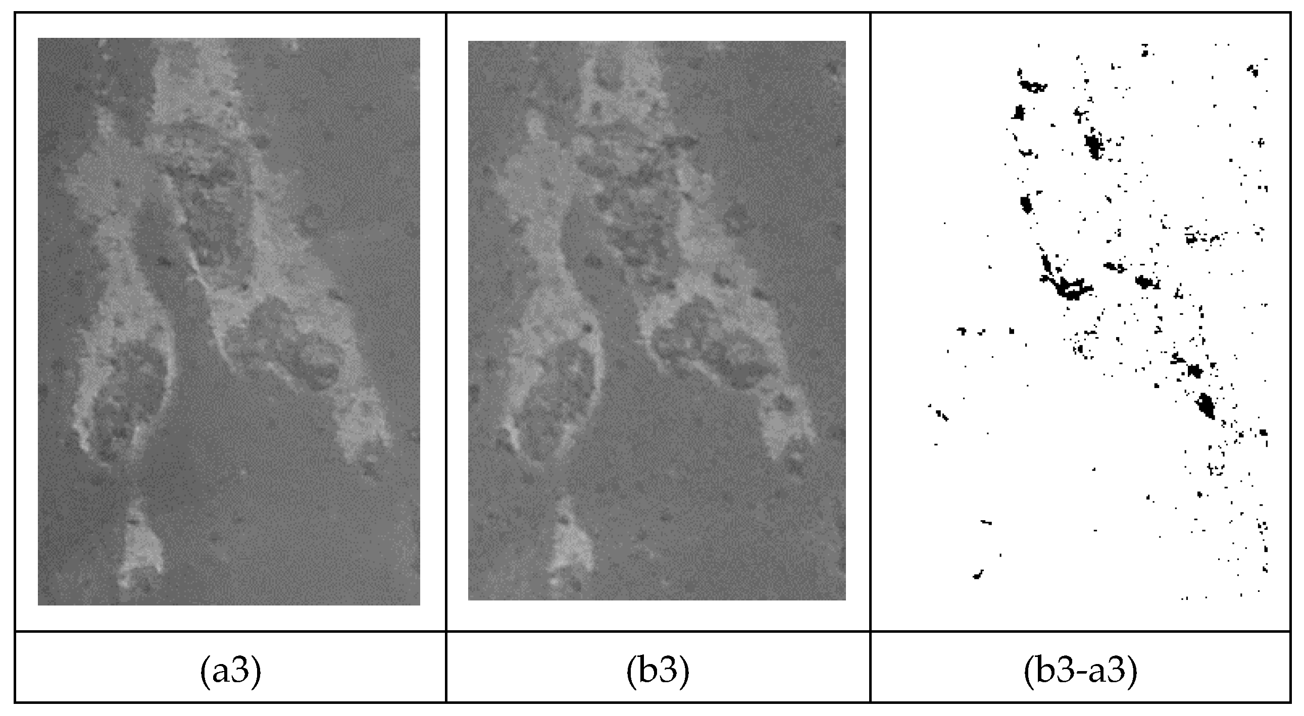
Figure 16 shows the zones 1, 2 and 3; in the first columns after 34 h of testing, named (a1), (a2), and (a3); and in the second column after 50 h of testing named (b1), (b2), and (b3). In the third column, the main differences between 34 and 50 h are indicated and presented as (b1-a1), (b2-a2), and (b3-a3). For each area, the percentage of eroded surface between 34 and 50 h of testing has been calculated by dividing the number of dark pixels by the total number of pixels, with the following results:
Area 1 (b1-a1): 1.21%;
Area 2 (b2-a2): 1.18%;
Area 3 (b3-a3): 2.33%.
3.3. Cavitation Power Indicator Results
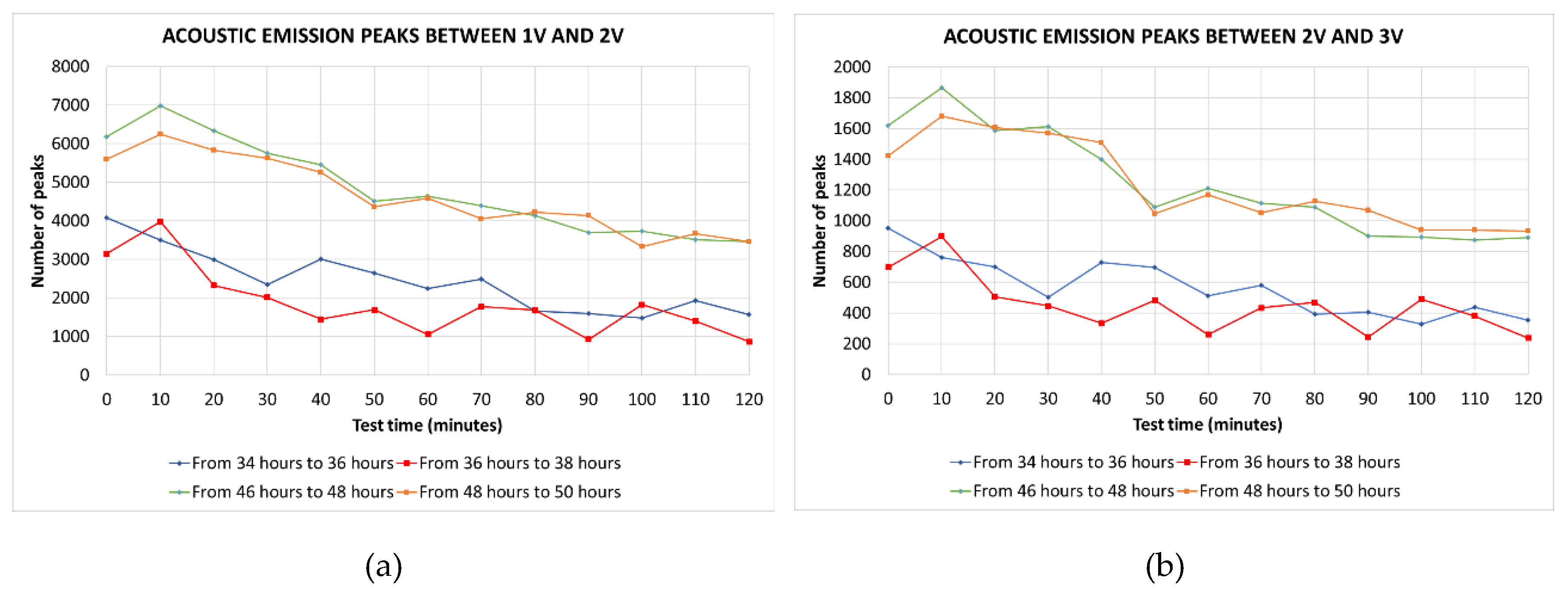
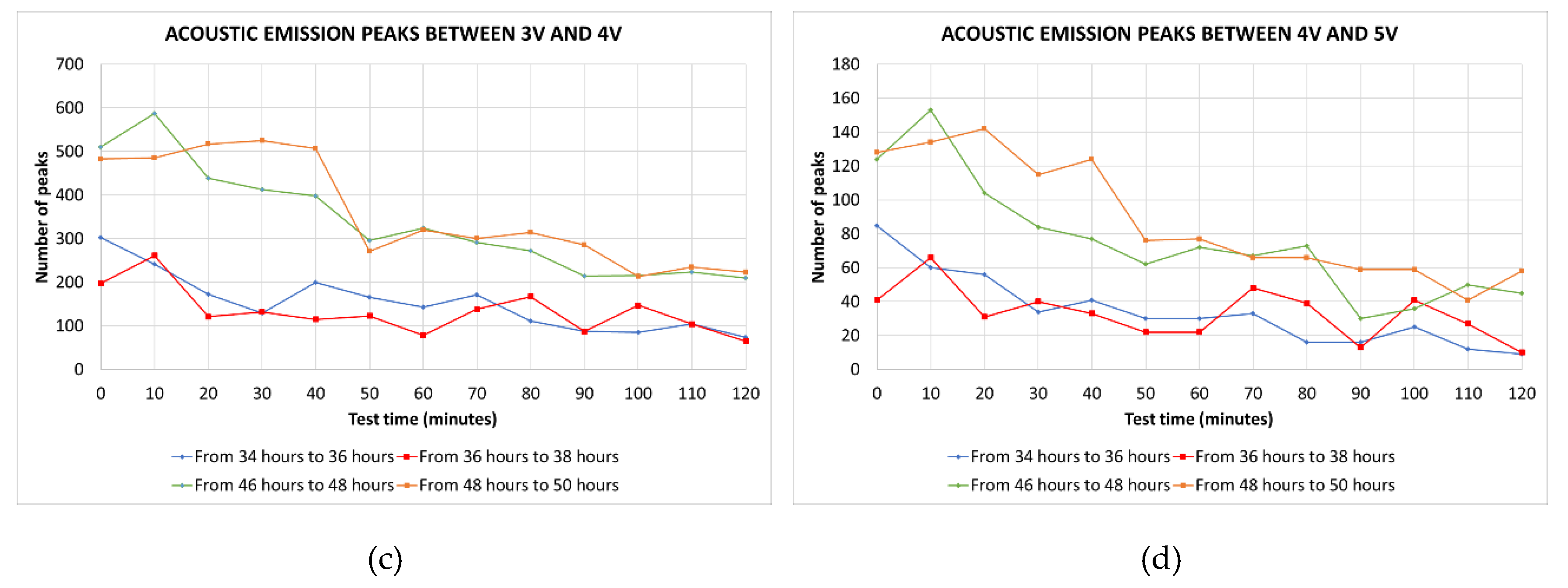
Figure 17 shows the evolution on time of the number of peaks corresponding to the clusters
,
,
, and
, as defined in
Section 2.4, corresponding to different AE measurements. It must be noted that the results from clusters
and
have not been shown because they only contained a few numbers of peaks which were not statistically significant.
Table 3 shows the mean values of the numbers of peaks corresponding to the different clusters of the tests studied.
On one hand,
Figure 16 shows that the numbers of peaks decrease over time in all short duration tests of 2h. Therefore, it can be concluded that, during a continuous test, the number of cavitation impacts decreases.
On the other hand, it is also observed that the number of peaks in the final tests is higher than in the intermediate tests. According to
Table 3, these increases range from 121.2% (cluster between 1 and 2 V) to 143.8% (cluster between 3 and 4 V). Therefore, it can be concluded that the number of cavitation impacts increases throughout the erosion process
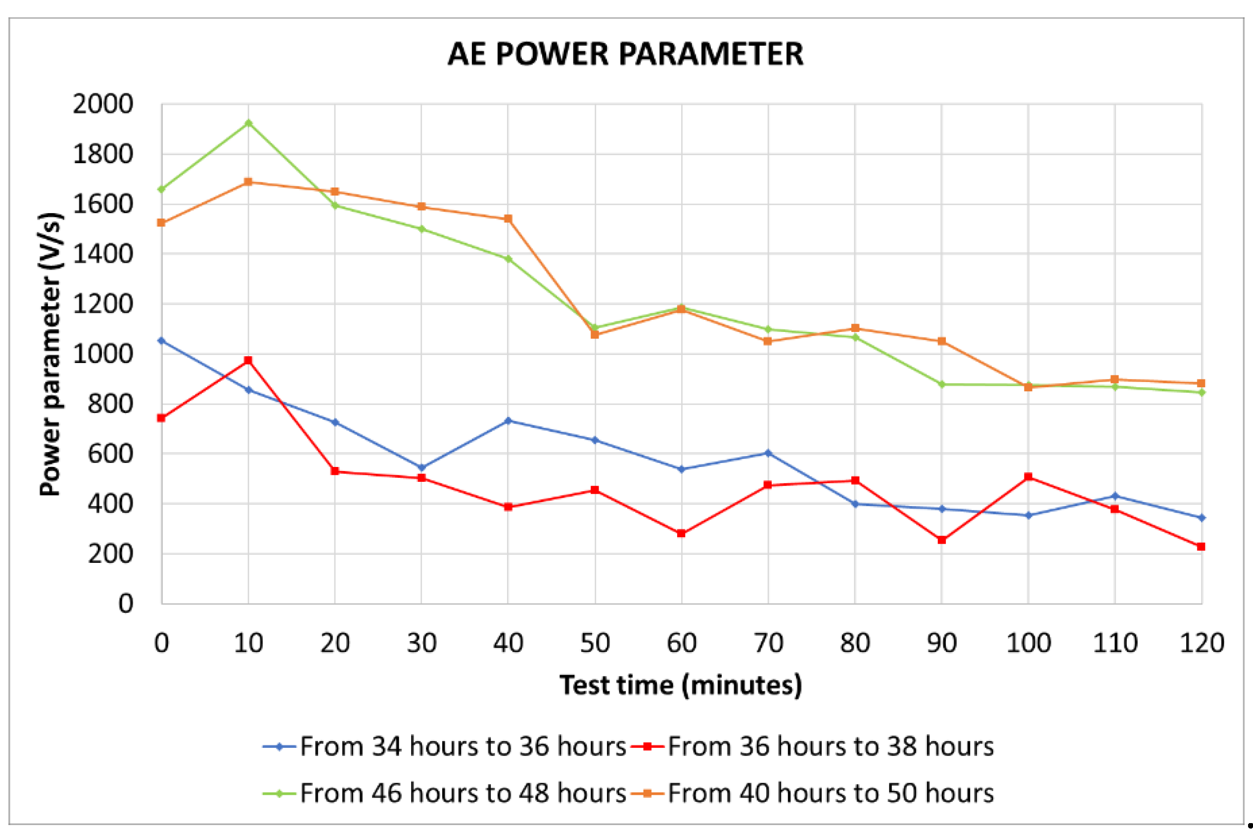
Figure 18 shows the temporal evolution of the power parameter defined in (2). This parameter is a global indicator of cavitation power (number of impacts multiplied by their squared level and divided by time).
Table 3 shows this parameter for the different tests in its last column, as well as the mean values for each group of tests.
Figure 18 indicates that, as before, the power parameter decreases throughout any continuous 2 h test. Moreover, the power parameter is significantly higher during the final tests at 50 h than during the intermediate tests at 38 h. According to
Table 3, this increase is of about 132.3%. It can be concluded that the power of cavitation impacts increases throughout the erosion process.
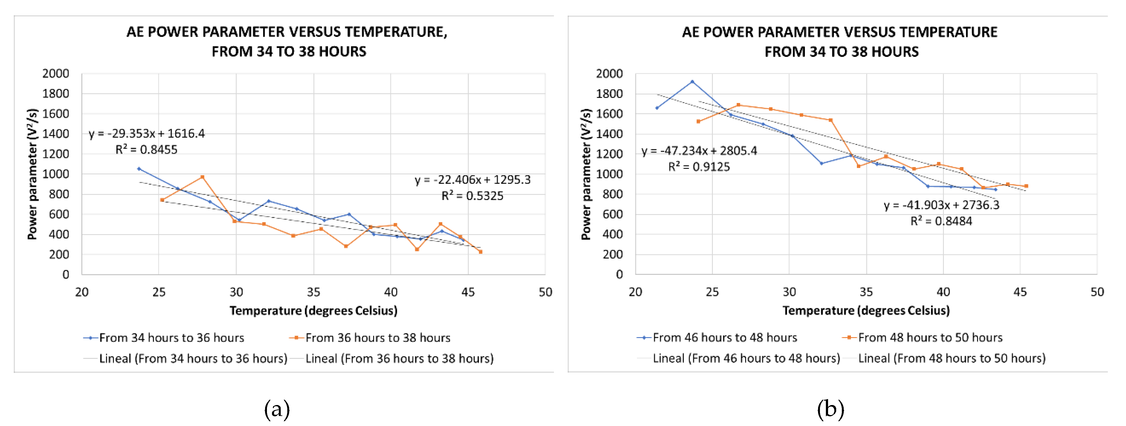
Figure 19 shows the power parameter versus temperature. The power parameter decreases when the temperature increases. In order to quantitatively evaluate the influence of temperature on the power parameter, straight lines have been fitted to the points corresponding to the different tests.
Table 4 shows the slopes of the different fitted lines and their mean values corresponding to the tests performed at the same conditions. The mean of the slopes corresponding to the intermediate tests is -28.9 °/(V
2/s) and the one corresponding to the final tests is -44.6 °/(V
2/s). So, the influence of temperature is greater in the final tests, when the extent of erosion is greater.
4. Discussion
A cavitation erosion test was carried out during 50 h in a cavitation tunnel with a Venturi equipped with an aluminum specimen and submitted to cloud cavitation. Hydraulic conditions (pressures and flow rate) were controlled to maintain a maximum cavity length between 70 and 110 mm during all the tests. The temperature increased during each short duration 2 h test because of the pump heating. This increase in temperature produced an increase in pressure which was controlled and kept constant by periodic manual purging of the air located in the upper part of the high-pressure tank.
During two specific time intervals from 34 to 38 h and from 46 to 50 h, AE measurements were taken every 10 minutes. At 38 and 50 h, photographs of the surface erosion were also taken. Three particularly damaged areas were selected to analyze the changes in surface condition between the two analyzed periods of time. The increase of eroded surface in these areas was of about 1.2%, 1.2%, and 2.3%, respectively.
The cloud cavitation shedding frequency was calculated from the AE measurements and it was found to be related with the cavitation number in a roughly linear way, which is consistent with the finding of Ylönen et al. [
5].
Based on the AE measurements, impacts grouped into classes by amplitude range were estimated, and a general "power parameter" was defined. It was then seen that that the mean number of impacts and the proposed new power parameter increased between the intermediate interval and the final one. Moreover, it was also seen that both the number of impacts and the power parameter decreased over the course of any of the short duration 2 h tests as the temperature increased continuously.
The increase in the mean number of impacts and the mean power parameter from one test to the next one after 12 hours of cavitation attack may be due to increased roughness induced by cavitation erosion. Hao et al. [
17] suggested that the cavity in a rough surface may rupture, detach, and collapse more than once over a period. This could explain the increase in cavitation impacts over time in our experiments.
The decrease in the number of impacts and the power parameter throughout a 2 h test could be due to the increase in temperature that occurs during the pump operation. Priyadarshi et al. [
14] studied the relationship between temperature and mass loss in two types of cast aluminum (A356.2 and A380) using ultrasonic cavitation. They found that mass loss increases with increasing temperature up to 30°C, followed by a decrease. Assuming that the number of impacts and the power parameter calculated from the AE are estimators of cavitation aggressiveness, and that the maximum erosion temperature of the studied aluminum (A 7075-T6) is unknown, as well as the moderate uncertainty produced by pressure oscillations, the finding of Priyadarshi et al. [
14] and the finding of the present work might be consistent.
To clarify the relationship between cavitation erosion and AE, new tests with better control of pressures and evaluation of erosion will be performed. In any case, this AE seems a promising technique for the evaluation of cavitation and its erosion, as well as for underlying the parameters affecting it such as the water temperature and the amount of erosion of the surface.
Author Contributions
Conceptualization, I.F-O. and X.E.; methodology, I.F-O., R.Z. and X.E.; software, I.F-O. and D.B.; validation, I.F-O. and X.E.; formal analysis, I.F-O.; investigation, I.F-O., D.B. and R.Z.; resources, X.E.; data curation, I.F-O.; writing—original draft preparation, I.F-O.; writing—review and editing, I.F-O. and X.E.; supervision, X.E.; project administration, X.E.. All authors have read and agreed to the published version of the manuscript.
Funding
This research received no external funding.
Data Availability Statement
Dataset available on request from the authors.
Acknowledgments
The authors wish to thank Mr. David Castañer for his help in setting up the cavitation tunnel, Ms. Elena Izquierdo for her collaboration in making the drawings of the test section and the team of the Barcelona Fluids & Energy Lab for their technical support and assistance.
Conflicts of Interest
The authors declare no conflicts of interest.
References
- Dular, M.; Ohl, C.D. Bulk Material Influence on the Aggressiveness of Cavitation – Questioning the Microjet Impact Influence and Suggesting a Possible Way to Erosion Mitigation. Wear 2023, 530–531, 205061. [Google Scholar] [CrossRef]
- Gogate, P.R. Application of Cavitational Reactors for Water Disinfection: Current Status and Path Forward. J. Environ. Manag. 2007, 85, 801–815. [Google Scholar] [CrossRef] [PubMed]
- Franc, J.P.; Michel, J.M. Cavitation Erosion. In Fundamentals of Cavitation; Kluwer Academic Publishers: Dordrecht, 2005; pp. 265–291. [Google Scholar]
- Grosse, C.U.; Ohtsu, M.; Aggelis, D.G.; Shiotani, T. Acoustic Emission Testing; Grosse, C.U., Ohtsu, M., Aggelis, D.G., Shiotani, T., Eds.; Springer Tracts in Civil Engineering; Springer International Publishing: Cham, 2022; ISBN 978-3-030-67935-4. [Google Scholar]
- Ylönen, M.; Franc, J.P.; Miettinen, J.; Saarenrinne, P.; Fivel, M. Shedding Frequency in Cavitation Erosion Evolution Tracking. Int. J. Multiph. Flow. 2019, 118, 141–149. [Google Scholar] [CrossRef]
- Schmidt, H.; Kirschner, O.; Riedelbauch, S.; Necker, J.; Kopf, E.; Rieg, M.; Arantes, G.; Wessiak, M.; Mayrhuber, J. Influence of the Vibro-Acoustic Sensor Position on Cavitation Detection in a Kaplan Turbine. In Proceedings of the IOP Conference Series: Earth and Environmental Science; Institute of Physics Publishing, 2014; Volume 22. [Google Scholar]
- Escaler, X.; Egusquiza, E.; Farhat, M.; Avellan, F.; Coussirat, M. Detection of Cavitation in Hydraulic Turbines. Mech. Syst. Signal Process 2006, 20, 983–1007. [Google Scholar] [CrossRef]
- Ylönen, M. Cavitation Erosion Monitoring by Acoustic Emission; Université Grenoble Alpes, 2020. [Google Scholar]
- Ylönen, M.; Saarenrinne, P.; Miettinen, J.; Franc, J.-P.; Fivel, M.C.; Fivel, M. Cavitation Bubble Collapse Monitoring by Acoustic Emission in Laboratory Testing. 2018. [CrossRef]
- Ylönen, M.; Saarenrinne, P.; Miettinen, J.; Franc, J.-P.; Fivel, M.; Laakso, J. Estimation of Cavitation Pit Distributions by Acoustic Emission. J. Hydraul. Eng. 2020, 146. [Google Scholar] [CrossRef]
- Fernández-Osete, I.; Bermejo, D.; Ayneto-Gubert, X.; Escaler, X. Review of the Uses of Acoustic Emissions in Monitoring Cavitation Erosion and Crack Propagation. Foundations 2024, 4, 114–133. [Google Scholar] [CrossRef]
- Hattori, S.; Goto, Y.; Fukuyama, T. Influence of Temperature on Erosion by a Cavitating Liquid Jet. Wear 2006, 260, 1217–1223. [Google Scholar] [CrossRef]
- Li, Z.; Han, J.; Lu, J.; Zhou, J.; Chen, J. Vibratory Cavitation Erosion Behavior of AISI 304 Stainless Steel in Water at Elevated Temperatures. Wear 2014, 321, 33–37. [Google Scholar] [CrossRef]
- Priyadarshi, A.; Krzemień, W.; Salloum-Abou-Jaoude, G.; Broughton, J.; Pericleous, K.; Eskin, D.; Tzanakis, I. Effect of Water Temperature and Induced Acoustic Pressure on Cavitation Erosion Behaviour of Aluminium Alloys. Tribol. Int. 2023, 189. [Google Scholar] [CrossRef]
- Dular, M. Hydrodynamic Cavitation Damage in Water at Elevated Temperatures. Wear 2016, 346–347, 78–86. [Google Scholar] [CrossRef]
- Escaler, X.; Dupont, P.; Avellan, F. Experimental Investigation on Forces Due to Vortex Cavitation Collapse for Different Materials. Wear 1999, 65–74. [Google Scholar] [CrossRef]
- Hao, J.; Zhang, M.; Huang, X. The Influence of Surface Roughness on Cloud Cavitation Flow around Hydrofoils. Acta Mech. Sin. /Lixue Xuebao 2018, 34, 10–21. [Google Scholar] [CrossRef]
- Bermejo, D.; Escaler, X.; Ruíz-Mansilla, R. Experimental Investigation of a Cavitating Venturi and Its Application to Flow Metering. Flow Meas. Instrum. 2021, 78. [Google Scholar] [CrossRef]
- Automation Creations Inc. Available online: https://Matweb.Com/Search/PropertySearch.Aspx.
- Bendat, J.S.; Allan, G. Piersol The Hilbert Transform. In Random data: analysis and measurement procedures; 2011; pp. 473–503. [Google Scholar]
Figure 1.
Cavitation tunnel of the Barcelona Fluids & Energy Lab where the tests were performed.
Figure 1.
Cavitation tunnel of the Barcelona Fluids & Energy Lab where the tests were performed.
Figure 2.
Test section of the cavitation tunnel with the venturi and cavitation.
Figure 2.
Test section of the cavitation tunnel with the venturi and cavitation.
Figure 3.
Venturi section and removable metallic test specimen.
Figure 3.
Venturi section and removable metallic test specimen.
Figure 4.
Water temperature measured during the tests at the high-pressure tank, and their corresponding fitted curves: (a) From hours 34 to 36 and from 36 to 38; (b) From hours 46 to 48 and from 48 to 50.
Figure 4.
Water temperature measured during the tests at the high-pressure tank, and their corresponding fitted curves: (a) From hours 34 to 36 and from 36 to 38; (b) From hours 46 to 48 and from 48 to 50.
Figure 5.
Evolution of the inlet pressure of the test section during the tests: (a) From hours 34 to 36 and from 36 to 38; (b) From hours 46 to 48 and from 48 to 50.
Figure 5.
Evolution of the inlet pressure of the test section during the tests: (a) From hours 34 to 36 and from 36 to 38; (b) From hours 46 to 48 and from 48 to 50.
Figure 6.
Sensor Vallen model 150-M fitted at the bottom of the test section.
Figure 6.
Sensor Vallen model 150-M fitted at the bottom of the test section.
Figure 7.
Procedure for calculating the shedding frequency from the measured AE. (a) Original and filtered time signals. (b) Original and filtered spectra. (c) Filtered signal and its envelope. (d) Envelope spectrum indicating the shedding frequency and its harmonic.
Figure 7.
Procedure for calculating the shedding frequency from the measured AE. (a) Original and filtered time signals. (b) Original and filtered spectra. (c) Filtered signal and its envelope. (d) Envelope spectrum indicating the shedding frequency and its harmonic.
Figure 8.
Example of peaks identified with amplitudes higher than 1 V from the envelope function obtained during 1 s of AE measurement.
Figure 8.
Example of peaks identified with amplitudes higher than 1 V from the envelope function obtained during 1 s of AE measurement.
Figure 9.
Evolution of the test section outlet pressure during the tests: (a) From hours 34 to 36 and from 36 to 38; (b) From hours 46 to 48 and from 48 to 50.
Figure 9.
Evolution of the test section outlet pressure during the tests: (a) From hours 34 to 36 and from 36 to 38; (b) From hours 46 to 48 and from 48 to 50.
Figure 10.
Evolution of the test pressure drop in the test section during the tests: (a) From hours 34 to 36 and from 36 to 38; (b) From hours 46 to 48 and from 48 to 50.
Figure 10.
Evolution of the test pressure drop in the test section during the tests: (a) From hours 34 to 36 and from 36 to 38; (b) From hours 46 to 48 and from 48 to 50.
Figure 11.
Evolution of the cavitation numbers in the test section during the tests: (a) From hours 34 to 36 and from 36 to 38; (b) From hours 46 to 48 and from 48 to 50.
Figure 11.
Evolution of the cavitation numbers in the test section during the tests: (a) From hours 34 to 36 and from 36 to 38; (b) From hours 46 to 48 and from 48 to 50.
Figure 12.
Shedding frequencies during the tests: (a) From hours 34 to 36 and from 36 to 38; (b) From hours 46 to 48 and from 48 to 50.
Figure 12.
Shedding frequencies during the tests: (a) From hours 34 to 36 and from 36 to 38; (b) From hours 46 to 48 and from 48 to 50.
Figure 13.
Shedding frequencies versus cavitation numbers during tests: (a) From hours 34 to 36 and 36 to 38; (b) From hours 46 to 48 and 48 to 50.
Figure 13.
Shedding frequencies versus cavitation numbers during tests: (a) From hours 34 to 36 and 36 to 38; (b) From hours 46 to 48 and 48 to 50.
Figure 14.
Sketch of the specimen surface showing the photographed areas, named as 1, 2 and 3.
Figure 14.
Sketch of the specimen surface showing the photographed areas, named as 1, 2 and 3.
Figure 15.
Detail of the projective transformation applied to a picture of a specimen taken from an arbitrary point (black line) that produces an image of the specimen taken from above the centre of the specimen (red line).
Figure 15.
Detail of the projective transformation applied to a picture of a specimen taken from an arbitrary point (black line) that produces an image of the specimen taken from above the centre of the specimen (red line).
Figure 16.
Photographs of areas1, 2 and 3 at 34 h: (a1), (a2) and (a3); at 50 h: (b1), (b2) and (b3); and the erosion occurred between both: (b1-a1), (b2-a2) and (b3-a3).
Figure 16.
Photographs of areas1, 2 and 3 at 34 h: (a1), (a2) and (a3); at 50 h: (b1), (b2) and (b3); and the erosion occurred between both: (b1-a1), (b2-a2) and (b3-a3).
Figure 17.
Evolution of the number of peaks corresponding to different clusters, corresponding to different AE measurements during the tests: (a) Cluster of peaks between 1 and 2 V; (b) Cluster of peaks between 2 and 3 V; (c) Cluster of peaks between 3 and 4 V; (d) Cluster of peaks between 4 and 5 V.
Figure 18.
Evolution of the power parameter during the tests.
Figure 18.
Evolution of the power parameter during the tests.
Figure 18.
Power parameter versus temperature during the tests.
Figure 18.
Power parameter versus temperature during the tests.
Table 1.
Initial and final temperatures of the different periods.
Table 1.
Initial and final temperatures of the different periods.
| Test |
Period |
Temperatures (Celsius) |
| |
|
Initial |
Final |
Increase |
| Intermediate |
34-36 hours |
23.7° |
44.7° |
21.0° |
| |
36-38 hours |
25.2° |
45.8° |
20.6° |
| Final |
46-48 hours |
21.4° |
43.4° |
22.0° |
| |
48-50 hours |
24.1° |
45.4° |
21.3° |
| Average |
|
23.6°
|
44.8°
|
21.2°
|
Table 2.
Minimum, maximum pressures at inlet and outlet test section, and their drop.
Table 2.
Minimum, maximum pressures at inlet and outlet test section, and their drop.
| Test |
Period (h) |
Pressure at the test section inlet (kPa) |
Pressure at the test section outlet (kPa) |
Drop pressure in the test
section (kPa)
|
| |
|
Max |
Min |
Range |
Max |
Min |
Range |
Max |
Min |
Range |
| Intermediate |
34-36 |
137.0 |
121.5 |
14.3 |
86.5 |
63.4 |
23.1 |
58.1 |
49.3 |
8.8 |
| 36-38 |
138.2 |
123.6 |
14.6 |
90.4 |
68.3 |
22.1 |
55.3 |
47.5 |
7.8 |
| Final |
46-48 |
137.1 |
128.6 |
8.5 |
88.4 |
75.4 |
13.0 |
53.4 |
48.7 |
4.7 |
| 48-50 |
136.9 |
127.7 |
9.2 |
87.2 |
73.9 |
13.3 |
53.7 |
48.7 |
5.0 |
| Average |
|
137.0 |
125.4 |
11.7 |
88.1 |
70.3 |
17.9 |
55.1 |
53.7 |
6.6 |
Table 3.
Number of peaks of the different clusters and power parameter.
Table 3.
Number of peaks of the different clusters and power parameter.
| Test |
Number of peaks within a cluster |
Power parameter
(V2/s)
|
| |
1 to 2 V |
2 to 3 V |
3 to 4 V |
4 to 5 V |
| From 34 to 36 |
2426 |
566 |
153 |
34 |
585 |
| From 36 to 38 |
1858 |
452 |
133 |
33 |
476 |
| Mean of intermediate tests |
2142 |
509 |
143 |
34 |
531 |
| From 46 to 48 |
4830 |
1242 |
338 |
75 |
1229 |
| From 48 to 50 |
4646 |
1236 |
360 |
88 |
1237 |
| Mean of final tests |
4738 |
1239 |
349 |
82 |
1233 |
| Increase from intermediate to final tests |
121.2% |
143.4% |
143.8% |
141.1% |
132.3% |
Table 4.
slopes of the different fitted lines and the averages corresponding to the tests performed at the same conditions.
Table 4.
slopes of the different fitted lines and the averages corresponding to the tests performed at the same conditions.
| Test |
Period (h) |
Straight line slope°/(V2/s)
|
Slope average°/(V2/s)
|
| Intermediate |
34-36 |
-29.4 |
-28.9 |
| 36-38 |
-28.4 |
| Final |
46-48 |
-47.2 |
-44.6 |
| 48-50 |
-41.9 |
|
Disclaimer/Publisher’s Note: The statements, opinions and data contained in all publications are solely those of the individual author(s) and contributor(s) and not of MDPI and/or the editor(s). MDPI and/or the editor(s) disclaim responsibility for any injury to people or property resulting from any ideas, methods, instructions or products referred to in the content. |
© 2025 by the authors. Licensee MDPI, Basel, Switzerland. This article is an open access article distributed under the terms and conditions of the Creative Commons Attribution (CC BY) license (http://creativecommons.org/licenses/by/4.0/).