
Submitted:
13 February 2026
Posted:
14 February 2026
You are already at the latest version
Abstract
The literature indicates that the qubit requirements for factoring RSA-2048 remain on the order of 1 million, under commonly assumed architectures and error-correction models, leaving a substantial gap between current resource estimates and near-term practical feasibility. Reducing this requirement to the low thousands qubit regime therefore remains an important open research objective. This work proposes a hybrid classical-quantum algorithm using a classical modular exponentiation subroutine with a Quantum Number Theoretic Transform (QNTT) circuit, to increase the speed and reduce the number of quantum components, including gates and qubits, to factor integer numbers, which serve as keys in cryptographic methods, like RSA and ECC, when compared with Shor’s algorithm. Several composite numbers, the result of multiplication of two primes, were validated through both simulation and real quantum hardware by benchmarking the full Shor pipeline on simulation and on a real IBM quantum computer. In simulation, the proposed Jesse–Victor–Gharabaghi (JVG) algorithm achieved substantial practical reductions in computational resources, decreasing runtime from 174.1 s to 5.4 s, memory usage from 12.5 GB to 0.27 GB, and quantum gate counts by approximately 99%. Because Shor and JVG use different register sizes for the same composite N, the reported gate/depth reductions should be interpreted as end-to-end quantum-resource budgets to factor the same N, rather than a per-qubit or transform-only efficiency claim. On quantum hardware, JVG reduced the required runtime from 67.8 s to 2 s, and the quantum gate counts by over 98%. Projection for RSA-2048 indicates that the JVG algorithm significantly outperforms Shor’s approach, requiring a projected quantum runtime of 11 hours for a factorization under identical scaling assumptions. The results from these evaluations support JVG as a more hardware-compatible and robust noise-tolerant substitute for Shor’s framework, offering a viable path toward practical quantum integer factorization on near-term Noisy Intermediate-Scale Quantum (NISQ) devices.
Keywords:
quantum number theoretic transform
; quantum Fourier transform
; integer factorization
; Shor’s algorithm
; NISQ devices
1. Introduction
Quantum computing systems are anticipated to surpass their classical counterpart by implementing quantum mechanical principles like superposition, entanglement, and interference [1,2]. Driven by this potential, Quantum Computing has been attracting the attention of researchers and investors alike. Funding for the development of quantum technologies, from both public and private investors, increased 54% between 2023 and 2024, reaching US$2.0 billion worldwide, and is expected to reach around US$16.4 billion by 2027 [3,4]. This trend is also reflected in the rapid growth of quantum-focused companies such as D-Wave, IonQ, and Quantinuum, which have increased their market value by more than 2,530%, 800%, and 812%, respectively, over the past 12 months, reaching a combined market capitalization of approximately US$50 billion [5,6,7]. The massive investments in this sector have enabled significant advancements in multidisciplinary fields, such as finance [8,9], materials science [10,11], chemistry [12], pharmacology and health sciences [13,14], and machine learning [15,16].
Another major area impacted by quantum technology is cryptography [17,18,19]. Since Shor proposed a new algorithm using quantum information processing for efficient number factoring back in 1994 [20], his work proved the feasibility of a quantum-based algorithm for number factoring. By using modular exponentiation and the Quantum Fourier Transform (QFT), previously conceived by Coppersmith [21], Shor’s algorithm successfully captured the period of a function given an initial superposition state. By leveraging these components, this algorithm performs in polynomial time , in opposition to the exponential time required by the classical procedures for RSA integer factorization [22,23]. The creation of this algorithm demanded a novel way to tackle quantum-based hazards [24].
Building upon this knowledge, several subsequent studies sought to improve Shor’s algorithm. In [25], the authors focused on speeding up the arithmetic operations by using improved adder designs, allowing the parallel execution of quantum gates, while also optimizing the overall circuit’s structure. By doing so, they improved modular exponentiation performance by up to 700 times compared with existing approaches. Building upon the knowledge developed by Meter and Itoh [25], the authors in [26] proposed a new reversible circuit for modular exponentiation using linear-size circuits, and working on a register-transfer level instead of the commonly used qubit-transfer level. Their methodology’s overall performance showed better scalability than previously available methods, requiring four times fewer qubits.
The work by Ekerå [27] proposed changes to the QFT algorithm and the post-processing part alike. The author introduced a Shor’s discrete logarithm variant that is optimized when the discrete logarithm is significantly smaller compared to the group order . The algorithm uses smaller QFTs whose sizes reduce the total qubit requirements in this setting. Furthermore, instead of the classical continued fractions method used in Shor’s post-processing, the author employed lattice-based techniques to recover the discrete logarithm from the quantum measurement outcomes. This work has been further expanded in the following work by Ekerå and Håstad [28], where the authors showed that the RSA factorization can be formulated as a short discrete logarithm, thus reducing the burden on quantum computers.
Chevignard et al. [29] optimized the number of required logical qubits for Shor’s algorithm by providing an alternative algorithm for the modular exponentiation part. By combining Ekerå–Håstad’s algorithm, compression techniques and residual arithmetic, the authors could reduce the number of logical qubits required for RSA integer factoring. However, this simplification introduces a trade-off between the total number of qubits and the number of gates necessary for its implementation. Gidney [30] provides a review on the progress of factoring RSA-2048 using optimized, fault-tolerant variants of Shor’s algorithm. The author focused on minimizing logical qubit counts and circuit depth by combining algorithmic refinements, advanced quantum arithmetic, and lattice-based post-processing techniques, while explicitly accounting for surface-code error correction. Under optimistic physical error rates, the work estimates that RSA-2048 factorization would require in the order of hundreds of thousands of logical qubits, corresponding to fewer than one million noisy physical qubits, and would take up to days to execute.
Other methodologies investigated different combinations of classical and quantum subroutines to factor composite numbers, which are integers produced as a result of the product of two prime numbers. This strategy has been reported in several studies [31,32,33]. By combining both classical and quantum frameworks, a significant reduction in the computational burden for Shor’s factorization was achieved, proving the feasibility and utility of such an approach.
As the literature mentions, there are many efforts in different areas of Shor’s algorithm components, ranging from modular exponentiation to post-processing. However, a common feature of these works is their reliance on the QFT circuit or its variants for period extraction. Therefore, it remains necessary to investigate alternatives to the QFT structure itself. For example, alternative transforms may be more practical on quantum hardware for specific applications. One strong contender for this task is the Number Theoretic Transform (NTT), a specialized variant of the DFT that operates over finite fields via modular arithmetic rather than complex numbers [34,35]. Classically, the NTT runs in time and avoids floating-point precision issues, making it well-suited to cryptographic computations [36]. A quantum version of the NTT could, in principle, serve as a substitute for the QFT in algorithms involving integer or polynomial structures. Such an implementation might offer advantages in precision and potentially simpler gate constructions, since modular addition can be easier to realize than arbitrary quantum rotations, especially in the current noisy quantum computer architectures.
In this context, incorporating a quantum version of the NTT within a quantum framework could lead to a modular design of QFT circuits. By breaking down the QFT into smaller components and selectively substituting them with specialized transforms, the overall circuit can be simplified and made more efficient for NISQ hardware. Such modularization not only streamlines the implementation of fundamental quantum algorithms but also improves their adaptability and performance [37]. Modular QFT architectures support more efficient Quantum Phase Estimation (QPE), a key subroutine in many quantum applications such as quantum chemistry, Hamiltonian learning, and Variational Quantum Eigensolver (VQE) [38]. Decomposing QFT into optimally connected building blocks helps to overcome limitations in qubit connectivity, mitigate gate errors, and reduce decoherence, thereby enabling algorithms to tackle larger instances and deeper circuits [39]. Additionally, this strategy enables dynamic error mitigation and adaptive allocation of quantum resources, thereby enhancing the reliability and scalability of computations on available quantum devices.
Additionally, to the best of the authors’ knowledge, an effort of a purely classical computation of the phase estimation part of the factorization algorithm is yet to be addressed by the specialized literature. This is a crucial point to be addressed, since the quantum modular exponentiation is the most computationally demanding part of the factorization algorithm as proposed by Shor [40]. In this case, it is expected that by conveying part of the quantum algorithm into a classical framework, it could not only enable faster quantum computations but also factorize larger composite numbers on currently available quantum machines.
The reviewed literature indicates that the qubit requirements for factoring RSA-2048 remain in the order of 1 million, under commonly assumed architectures and error-correction models, leaving a substantial gap between current resource estimates and near-term practical feasibility. Reducing this requirement to the low thousands qubit regime therefore remains an important open research objective. To bridge this knowledge gap, we introduce a novel hybrid classical-quantum factorization algorithm, named Jesse-Victor-Gharabaghi (JVG) algorithm, separating the portions of the processing that can be effectively executed in classical computers, from the complex period finding that can be more effectively handled by quantum circuits. This way, the novel architecture incorporates a purely classical modular exponentiation subroutine, followed by a Quantum Number Theoretic Transform as an alternative to the usual QFT circuit. It is important to emphasize that JVG’s novelty lies in advancing number theory period finding by extracting it from a finite ring rather than a complex field.
The present work constitutes the first empirical validation of a hybrid QNTT-based approach through comprehensive benchmarking on both simulated and real quantum backends. This includes resource scaling projections under realistic NISQ constraints. This methodology offers a distinct and measurable contribution beyond previous QNTT formulations, which were neither integrated into nor tested within a complete quantum factoring framework.
At this stage of the study, the comparison will be limited to the proposed QNTT-based circuit and the standard Shor’s algorithm using QFT, as provided by IBM, which is our gold standard. This is so we have a clear baseline for evaluating performance and scalability. By establishing a direct comparison, it becomes possible to quantify the resource savings and noise resilience provided by the QNTT circuit, while maintaining the same algorithmic framework.
To keep the comparison interpretable, we use two baselines: (i) IBM’s reference Shor implementation (including controlled modular exponentiation and IQFT) and (ii) a matched hybrid baseline in which modular-exponentiation values are generated classically and embedded, while the transform block is IQNTT. This lets us isolate the effect of choosing IQFT vs. IQNTT within the same hybrid workflow, while still reporting end-to-end results against IBM’s full Shor pipeline.
Additionally, to the best of the authors’ knowledge, the specialized literature has not yet examined a Shor-like factorization workflow in which the modular-exponentiation values used for period estimation is generated in a purely classical subroutine and then encoded into a quantum register for the subsequent spectral step. Because quantum modular exponentiation is widely recognized as the dominant computational bottleneck in Shor’s algorithm [36], we introduce a hybrid classical–quantum factorization workflow, named the Jesse–Victor–Gharabaghi (JVG) algorithm, that delegates modular-exponentiation value generation to a classical routine and then performs quantum period estimation via a transform-and-measurement stage. In JVG, this transform stage is implemented using a Quantum Number Theoretic Transform (QNTT) circuit as an alternative to the conventional inverse Quantum Fourier Transform (IQFT).
2. Methodology
2.1. Quantum Fourier Transform
The Quantum Fourier Transform was conceived by Coppersmith [21]. It is the quantum counterpart of the classical Discrete Fourier Transform (DFT), mapping data from the time domain into the frequency one. Classically, DFT has complexity with the following formulation [34,41]:
Equation 1 shows the output vector as being a normalized linear combination of elements of the input vector . The term is the kernel of the transform function, given in terms of indices and , and by the vector length itself. According to Euler’s equation, this term can be understood as a combination of the oscillatory influence of sine and cosine at different frequencies, as given by . Additionally, by using advanced algorithm building techniques, it is possible to implement a faster variant of DFT with complexity , being this version often referred to as Fast Fourier Transform (FFT) [42]. The QFT is mathematically defined as [43,44]:
In expression in equation 2, the input quantum state is mapped into a superposition of states . Additionally, being this a quantum transformation, it lies within a Hilbert space with dimension N. As a unitary operation over an N-dimensional Hilbert space, QFT performs a linear transformation that preserves inner products and vector norms, ensuring reversibility within the dynamics of a quantum computer [43]. The quantum circuit for a 4-qubit configuration for QFT is presented in Figure 1.
Figure 1 elucidates that the QFT circuit is a sequence of rotations applied over a superposition state. From left to right, the first quantum Hadamard gate puts the qubit into superposition. It is then followed by controlled gates , which moves the qubit around the Z-axis given a angle. The last two operations are SWAPs, reversing the qubits orders to match the QFT’s definition [43,45].
2.2. Number Theoretic Transform
The Number Theoretic Transform (NTT) is a specialized version of DFT. While the latter operates over complex numbers, the former performs analogous computations over a real finite field or ring, often the integer modulus of a prime [46]. Its formulation is presented in equation 3 [35]:
Where indicates modular operations over a ring defined by a prime number , as in . Modular arithmetic operations then map the results into the defined ring by taking the remainder upon division by . This makes the values wrap around whenever they exceed this prime number [47]. Still in equation 3, the term represents the primitive root. In arithmetic, primitive roots generate the set of integer coprime values to the prime through successive exponentiations. Additionally, it is needed that and the primitive root must ensure that while , [47].
Given its similar formulation to the DFT, NTT can be implemented classically to reach complexity [48]. This is achieved by implementing the Gentleman-Sande algorithm [49]. Originally conceived as a variation of the Cooley-Tukey FFT algorithm [50], the Gentleman-Sande algorithm works in bit-reverse order, performing a decimation-in-frequency (DIF) factorization of the NTT. In this approach, the input sequence is processed in an orderly manner, but the outputs are produced in digit-reversed order. Each stage of the algorithm recursively breaks the problem into smaller parts, combining results using butterfly operations and twiddle factors (i.e., the unitary roots). The bit-reversal step must then be unscrambled at the end to recover the coefficients in the correct order. This variant, alongside Cooley-Tukey’s decimation-in-time (DIT) approach, forms one of the two standard recursive FFT factorizations, and is frequently adapted in NTT applications due to its memory efficiency and modular structure [42,49].
2.3. Quantum Number Theoretic Transform
Building upon the classical NTT and the Gentleman-Sande algorithm, the Quantum Number Theoretic Transform (QNTT) was developed to be used in a quantum framework. The original QNTT implementation used in this study was proposed by Lu et al. [51]. Their methodology combined quantum arithmetic operations together with quantum modular operations to implement a quantum version of the Gentleman-Sande butterfly operation for a configuration using four qubits as input and a modulus equal to 5. The authors implemented their QNTT circuit using NISQ friendly operations. For example, the adder and subtractor gates are composed of sequences of CNOT gates, which is more efficiently implemented than, for example, the QFT-based adder drapper [52,53,54,55]. By doing so, Lu et al. [51] developed an efficient quantum circuit able to perform QNTT operations in a quantum framework. Figure 3 depicts the QNTT circuit.
In Figure 3, the rectangular boxes represent the operations applied to the qubits. In this image, there are two input values represented by registers and, each one containing n-qubits. The register is the integer prime number determining the ring , containing n-qubits. The remaining registers, and are ancilla qubits that will help to compute the necessary operations, containing n-qubits each [51].
It can be observed that the QNTT circuit uses quantum modulus, addition, and subtraction operations to compute the transforms. It starts with a modulus operation computing , where the result is stored in a register using a CNOT gate. Then, the modular operation for the second input value is computed, and its result is stored in . The next adder and modular operations then compute , which returns the transformed value for the register . The last three operations compute , finally, it returns the transformed value for the second input register.
2.4. Shor’s Algorithm
Shor’s algorithm was designed to factor a composite number that is the product of two prime integers. This is done by finding the order such as , being the composite number to be factored and a random initial value. The quantum circuit for the order-finding used in Shor’s algorithm is shown in Figure 4.
Figure 4 can be split into three main structures. The first consists of putting the first register , initialized in state , into superposition. After that, the quantum modular exponentiation is applied to the circuit via controlled rotations. Here, the controls are the qubits in register and the targets are the qubits in register , initialized in state . Note that the number of qubits in register determines the size of the superposition, which impacts the phase estimation. In contrast, the number of qubits in needs to be sufficiently large to store integers up to . The last part of the circuit is the inverse QFT in the register. At the end of this circuit, the register is measured, revealing information about the period of the function [20,43,45].
2.5. The New Proposed Algorithm
As depicted in Figure 4, the modular exponentiation algorithm is exclusively quantum-based in the original implementation of Shor’s. In this study, we propose a purely classical computation of modular exponentiation, thereby reducing the quantum computational resources required to factorize composite numbers. In this methodology, the results for for a set of values are stored classically and then mapped into a complex Hilbert space. This mapping allows for the usage of the previous classical information within the proposed JVG quantum framework [15,16]. The proposed methodology is summarized in Figure 5.
In this study, the modular exponentiation values were computed classically using NumPy and then encoded into the quantum circuit using amplitude encoding as a data-embedding step [16]. After applying the inverse transform block and measuring the transform register, we use the dominant peak location(s) to form candidate orders, which are then verified classically by checking whether . Once a valid even order is found, we compute candidate factors using and repeat with more shots and/or a new co-prime (x) if the result is trivial.
For the quantum period, finding the JVG algorithm substitutes the IQFT circuit with the IQNTT. The novel quantum circuit for integer factorization in a quantum framework is presented in Figure 6.
Different from QFT in Shor’s algorithm, the IQNTT retrieves the period of a given function directly over a finite ring . By changing spectral estimation from the complex domain to a ring-based spectrum, we extend the number-theoretic formulation of period finding, offering a further understanding of its implementation.
Additionally, the QFT circuit requires extensive qubit interactions, which is difficult to implement on present quantum hardware. Noisy Intermediate-Scale Quantum (NISQ) devices have limitations such as reduced coherent time per qubit, high error rates per gate, i.e. gate operation errors and gate fidelity, and restricted connectivity, all of which make feasibility of QFT circuits [56,57]. Conversely, the QNTT circuit (Figure 3) avoids rotations in the input transformation, offering a simpler design. In this context, less complex implementations such as QNTT are preferable, as they offer a more efficient hardware-compatible framework for the current quantum devices [58].
For the IBM Shor baseline, we benchmark the complete order-finding circuit (superposition, controlled modular exponentiation, IQFT, and measurement). For the hybrid JVG workflow, modular-exponentiation values are generated classically and embedded, and we benchmark the quantum portion starting from the embedded state, comparing IQFT vs. IQNTT under identical settings.
We understand that the removal of would mask the true depth, connectivity stress and error accumulation that determines its feasibility on NISQ devices. This way, the reported hardware and transpiled metrics are meaningful for NISQ devices, while also being able to provide realistic resource forecasts.
Finally, for the benchmark, we assess resource growth for both simulated and empirical data using log-log plots. The fits and slopes are used to compare practical growth rates between the two frameworks at realizable sizes and RSA relevant scenarios, revealing practical scaling relevance under current NISQ constraints.
3. Results
To evaluate the performance of the proposed methodology, we conducted experiments using two different approaches. The first one used the Qiskit SDK to simulate the quantum circuit on a classical device. Table 1 has information about the hardware used for quantum simulations in a Windows 11 operating system.
The first part consisted of simulating both Shor’s and JVG on Qiskit AER simulator. To this end, we selected different composite numbers ranging from 2 to 75 digits. Selecting these values is necessary to assess the algorithms’ performance on composite values with different numbers of digits. For each one of these values, the total number of qubits used in the circuit also changes. The implemented Shor’s algorithm could not factor numbers larger than 5 digits. We also experimented with larger composite numbers, but due to hardware limitations, given that simulating quantum operations in classical devices is still very demanding [59,60], the Shor’s algorithm failed to run. However, given JVG’s hybrid configuration, it was possible to reduce the computational burden and use less resources during simulation, which allowed us to investigate the algorithm’s performance for larger composite numbers up to 75 digits. This large composite number was selected because we wanted to show the proposed algorithm’s performance using a similar circuit size comparable to the largest instance achieved by Shor’s. This choice allows a more direct and meaningful comparison between the two methodologies.
The second part involved implementing the same algorithms on an IBM quantum computer using the same numbers. At this stage, it is relevant to note that both methodologies compared the JVG against the Shor’s algorithm implemented by IBM [61], which here will be considered the gold standard for evaluations.
While the present results do not target many factorizations, i.e. RSA-2048, they establish a clear trajectory of improvement, indicating that the same principles could translate into significant resource savings in the given NISQ era. Table 2 contains information on the number of digits of the composite numbers, and whether they were factored or not using each algorithm. Henceforth, whenever two-digit numbers are presented in the following tables, they will be listed in ascending order.
To maintain clarity between simulated and experimental outcomes, all performance metrics in this work are reported within their native execution contexts. The simulation-based results use Qiskit’s gate model with the CX and U primitives, along with wall-clock execution time and RAM (memory) consumption as system-level metrics. These measurements capture algorithmic behavior independent of hardware-specific constraints. Conversely, the quantum computer evaluations are based on IBM Q backends that utilize a different native gate basis, primarily SX, CZ, and RZ, and we also report the Qiskit Runtime (QR) wall-clock time returned by the runtime service as a practical indicator of end-to-end execution demand. Because QR can include system-level overheads beyond the circuit itself (e.g., service/runtime orchestration and compilation effects), we use it primarily for within-setting comparisons and trend analysis, while native gate counts remain the primary hardware-independent resource indicators. This ensures that simulator results reflect algorithmic scaling properties, while hardware results capture physical implementation behavior under realistic noise and transpilation conditions.
3.1. Results for Quantum Simulation
To account for stochastic effects in the simulation, each experiment was repeated 10 times. The mean and standard deviation were computed for every configuration across these runs. The average coefficient of variation is reported in Table 3 for both approaches.
Results from Table 3 reveal a substantial performance advantage of JVG’s algorithm compared to Shor’s implementation. Most notably, it is noticeable that the proposed methodology was able to address the factorization of significantly larger numbers containing up to 75 digits. This reflects directly on the total amount of qubits used in each circuit. For Shor’s, the number of qubits increased as the composite number increased. However, this relationship is not necessarily true for JVG’s approach. For example, from Table 4, we can observe that JVG’s circuit size did not change for factoring 15, 21, 143 and 1363, where all of them needed only a 6 qubit-long circuit. Furthermore, considering the largest composite number for both algorithms, there is a significant difference in the number of qubits. While Shor’s algorithm required 70 qubits to factor a 5-digit composite number, the JVG approach required only 6 qubits to execute the circuit corresponding to the same number, a difference of over 90% in qubit count.
As a direct implication of the circuit size, the simulation time will also differ significantly. The data in Table 3 also reveal that JVG uses significantly less resources than the original Shor’s algorithm. Figure 7 and Figure 8 show the plot for the time and memory (RAM) metrics using Log10 scale. Note that the x-axis uses the number of digits required to factor each composite, not the composite number itself. These plots should be read as resources required by each pipeline to factor the tested instances, not as a matched-qubit comparison.
Figure 7 and Figure 8 reveal a clear divergence in scaling behavior between the two approaches. Over the measured range, the JVG pipeline exhibits an approximately linear growth trend, in the Log-Log plot, with respect to the number of digits, as indicated by the best-fit regression, while Shor’s implementation displays a markedly steeper growth consistent with exponential-like behavior under the same fitting procedure. This resulted in the JVG model requiring around 76 s to finish the factorization of a 75-digit composite number, compared to 170 s for Shor’s to factor a 5-digit-long instance, 55% less time per simulation run. Considering a 5-digit composite number, JVG alternative shows improved RAM usage, requiring on average 267 MB of memory, compared to 12.5 GB for the Shor quantum circuit, 98% lower RAM usage between the two approaches. Considering the largest composite number for JVG, the RAM usage was around 345 MB, which remains substantially lower than the values reported by Shor’s in the simulated outcomes.
The gate count also reveals that number factorization using the JVG circuit has superior scalability than the traditional Shor’s circuit. Still considering the 5-digit-long case, JVG reduced the number of CX and U gates by 99% compared to the traditional Shor’s. Furthermore, direct assessment on the data in Table 3 reveals better scalability for JVG’s methodology. This implies that the total computational resources will increase, but at a slower rate than Shor’s algorithm.
Considering the variation in resource usage from the smallest to the largest composite number successfully factored by both algorithms, it is possible to observe how each approach scales as the circuit size increases. For instance, Shor’s circuit exhibited an increase of 172 times in runtime and nearly 29 times for RAM consumption considering this interval. JVG, in turn, increased 1.5 times considering the run time, while the memory presented a small variation of 2%, remaining stable. For gate count, the most significant difference is observed for the U gate, which increased by over 175 times for Shor, while JVG increased nearly 3 times for this same indicator.
As previously stated, Shor’s algorithm, under the same experimental and hardware constraints, could not be executed for composite numbers larger than 5 digits due to prohibitive computational and memory requirements. On the other hand, JVG’s algorithm was able to factor the corresponding composite numbers. This distinction is a significant cornerstone, as it is possible to verify the algorithm’s performance beyond Shor’s feasibility and gaining access to information related to data performance, resource scaling and noise sensitivity. Consequently, these results demonstrate that the proposed JVG algorithm has space for further improvements that may lead to successful runs at scales currently unattainable by fully quantum algorithms.
3.2. Results for Implementation on a Real Quantum Hardware
We also repeated the circuits ten times when implementing the circuits in a quantum device. Different from the simulation methodology, we could not run the circuits for 5 digits for Shor’s algorithm. This was due to the current constraints of the NISQ devices. They still offer limited coherence time and qubit connectivity, which prevent more profound and more complex quantum circuits from being implemented. Given Shor’s configuration with a computationally expensive modular exponentiation quantum circuit, larger configurations proved to be unfeasible. Nevertheless, we managed to implement JVG’s algorithm for the same previously presented composite values, which offers a better take on the proposed methodology.
At this phase, the quantum device used in our methodology was “ibm_torino”, which uses the Heron R1 quantum processor and has 133 qubits. We recommend addressing reference [62] for further information on this device and its processor.
Additionally, for every configuration, the mean and standard deviation were calculated across these runs, in the same fashion previously described. Table 4 contains the results for implementing the algorithms.
In Table 4, both methodologies exhibited stable behavior across repeated runs, with relative standard deviations remaining within a few percentage points of the mean. The inclusion of add/subtract blocks in the QNTT circuit, together with its hybrid architecture correlates with reduced numbers of gates SX, CZ and RZ. The same behavior was observed in the data in Table 3 for the simulated results. The JVG algorithm showed more stable runs concerning the QR variation, as its standard deviation was near zero across the assessed circuits, a significant improvement over the 3.80% reported by Shor’s algorithm. The JVG implementation maintained comparable variability for the primary quantum gate metrics, reaching 0.73% for SX, 0.82% for CZ, and 0.39% for RZ gates. The counterpart version reached 0.26%, 0.29%, and 0.33%, respectively.
Table 4 confirms the simulated results previously presented, where the proposed JVG algorithm managed to use less resources than the traditional Shor’s algorithm. Figure 9 presents the plots comparing QR versus the total number of qubits in the circuit for each composite number. Note that the following plots use the number of digits required to factor each composite number, not the composite number itself.
In Figure 9, the QR consumption associated with Shor’s algorithm follows a different empirical trend than that observed in Figure 7. In this case, the data are better described by a power-law fit rather than the exponential-like growth previously observed. By contrast, the JVG algorithm preserves an approximately linear growth profile, in the Log-Log plot, across both methodologies and experimental settings. Consequently, the increase in QR consumption for JVG remains close to linear with circuit size, whereas Shor’s implementation exhibits substantially steeper growth that is better captured by a power-law relationship in this regime. Across all evaluated composite numbers, JVG maintained a QR time well below 10 s. In contrast, Shor’s algorithm presented a significant variation in its QR-reported runtime, growing from 4 s to around 68 s between its initial and final configurations. A similar disparity is observed in quantum gate usage. Relative to the full Shor factoring pipeline for the same tested instances, the total quantum gate count is reduced by more than 99% in the JVG approach.
Moreover, Shor’s algorithm exhibited an approximately 16-fold increase in QR from its initial to its final configuration, whereas the QR associated with JVG increased by only a factor of three over a substantially larger problem-size. Circuit size followed a similar trend. As the composite number increased from two to four digits, Shor’s implementation expanded markedly from 18 to 46 qubits, leading to a rapid escalation in resource consumption, as shown in Table 4. By contrast, the JVG architecture displayed considerably more stable behavior, particularly for smaller composite numbers, and was able to execute circuits corresponding to a 75-digit composite number using a 70-qubit configuration. This reaffirms the intense resource consumption by Shor’s algorithm, compared to JVG, especially in terms of QR and qubit usage.
3.3. Projections for RSA Relevant Scenario
The goal of this extrapolation is to compare measured resource-growth behavior between the two pipelines, and not to claim a change in the known asymptotic complexity. These projections should therefore be interpreted as indicative scaling trends rather than precise forecasts, because extrapolation beyond the measured range is sensitive to error accumulation, compilation choices, and hardware-specific constraints that can change at larger qubit counts.
For clarity, we focus on a single cryptographically relevant reference point, namely RSA-2048. Importantly, the projected “QR time” reported represents an estimate of the quantum execution cost for a single order-finding attempt under the same experimental compilation/runtime context, rather than a guaranteed end-to-end wall-clock “time-to-break RSA” under all conditions. The total time-to-factor depends on the number of attempts required (e.g., repetitions over shots and/or co-prime choices of ) to obtain a usable order and nontrivial factors.
Considering that the same circuit size to factor RSA-2048 is used for both methodologies, we can observe a substantial divergence relative to Shor’s baseline in the projected quantum execution cost per order-finding attempt. For a cryptographic relevant quantum computer, Shor’s methodology is projected to demand years to factor RSA-2048 number, while JVG is estimated to require around minutes to perform the same task. Converting per-attempt values into an end-to-end “time-to-factor” requires accounting for the expected number of repetitions needed to recover a valid order and nontrivial factors; for example, one thousand attempts would scale the JVG estimates to roughly 11 hours, while preserving the large gap relative to the Shor baseline.
4. Discussion
Before interpreting these findings, it is important to clarify the conceptual scope of our contribution. The novelty of the JVG algorithm lies in its hybrid architecture, which combines classical modular exponentiation with a QNTT step, resulting in a compact quantum circuit. By removing the most resource-intensive components of the factoring pipeline to classical computation, i.e. the quantum modular exponentiation circuit, the quantum portion of the algorithm is reduced to a minimal and well-structured configuration that performs spectral analysis more efficiently than standard Shor’s, as observed in both simulated and experimental results.
4.1. Implications of Simulated Results for JVG’s Algorithm
The overall performance of the proposed JVG’s algorithm showed remarkable improvement over the standard Shor’s methodology, as observed in Table 3. JVG’s faster run time of quantum circuits is essential for the feasibility testing of the algorithm before moving to a real quantum device. The lower memory usage by JVG indicates better efficiency in terms of classical hardware use. This is of relevant interest given that currently, the simulation of quantum operations in classical devices is heavily constrained in memory usage [59,60]. Thus, more efficient algorithms offer a superior option for modelling and simulating more complex circuits.
Considering number factorization using Shor’s algorithm, the high amount of gates makes it hard to implement on the current noisy machines [58]. The proposed JVG methodology, combining a classical modular exponentiation subroutine with a QNTT structure, demonstrated improved scaling for quantum gate usage. The implementation of the proposed factorization methodology opens the way for a more NISQ-friendly alternative, in which scalability is essential [63]. Additionally, the proposed JVG algorithm offers more efficient simulations on classical backends, which remain an essential step for validating quantum algorithms before moving to a real quantum machine [64,65].
Therefore, the improvements achieved with JVG provide more tractable simulations of larger problem instances and a more realistic foundation for implementing integer factorization, while enabling significative savings on simulation cost per-run-basis.
4.2. Implications of Experimental Quantum Results for the JVG Algorithm
Considering the experimental data in Table 4, once again the JVG’s methodology managed to reach better metric indicators. Considering the QR metric, the proposed methodology requires less processing time and executes more efficiently, demonstrating that the JVG algorithm can better manage resource growth when implemented on real quantum devices. This is important for current NISQ machines, since they still lack a larger coherence time, thus preventing long computations [58,63]. In this context, it would be possible to implement factorization algorithms more efficiently for more complex circuits [28,66].
On real quantum hardware, such as IBM Quantum backends, operational cost is dominated by backend occupancy time, circuit depth, and the number of repetitions required to obtain a valid result, rather than by directly observable energy consumption. In this context, higher throughput and shorter quantum runtimes translate into lower effective cost per successful execution. Assuming identical experimental configuration, Shor’s algorithm needed 68 s to factor 4-digit long composite number, while JVG needed only 2 s. This represents a 97% reduction in effective backend occupancy time per run, under identical experimental configuration. This highlights the more efficient use of quantum hardware resources achieved by the JVG approach.
The reduced number of quantum gates in JVG’s configuration is particularly relevant in the current NISQ context. In particular, two-qubit controlled gates such as CZ are significant sources of error and reduced entanglement fidelity on quantum hardware when compared with single-qubit operations [67,68]. By mitigating their use, it is possible to obtain more reliable circuits in terms of both stability and noise resistance, which are highly desirable properties. When combined with reductions in single-qubit gates such as SX and RZ, these improvements enable shallower and more error-resistant implementations of number factorization algorithms.
The values presented in Table 4 should be regarded as indicative of performance trends rather than absolute benchmarks, as the experimental setup remains constrained by the current limitations of NISQ hardware. Likewise, percentage-based improvements on small baselines may exaggerate significance. Thus, this discussion focuses on comparative growth rates to assess true scalability and robustness.
Nevertheless, despite these hardware constraints, the experimental findings reinforce the robustness of the JVG methodology when implemented on real quantum devices, validating its projected trends observed in the experimental setup, further supporting the reliability and practical significance of the proposed approach for in NISQ computing applications.
4.3. Implications of the Projected Values for RSA Relevant Scenario
The RSA projections are entirely data-oriented and derived from the experimentally observed relationships between gate count and qubit number. They provide an evidence-based estimation of how both methodologies might behave under more complex circuit configurations, and for relevant scales, considering the experimental setup. The projected results indicate that the JVG algorithm sustains a markedly slower resource growth rate across all gate types and circuit-depth metrics compared to Shor’s framework. Specifically, they suggest that the JVG architecture maintains its scalability advantage even for RSA-size problems, reinforcing its potential as a more hardware-efficient, noise-resilient solution for future quantum cryptographic implementations. This behavior is already evident in the measured results presented in tables 3 and 4, where the JVG resource consumption exhibits an approximately linear increase with circuit size (and digit increase), in opposition to the growth observed for Shor’s algorithm. Therefore, JVG exhibits markedly slower empirical growth in run time and quantum gate count.
Interpreting the projected QR values as per-attempt quantum execution cost, the RSA-scale estimates still indicate an extreme separation between the pipelines: the Shor baseline grows into multi-year projected QR-time. At the same time, JVG remains in the seconds-to-minutes regime per attempt for the exact key sizes. The end-to-end “time-to-factor” then follows by multiplying these per-attempt values by the expected number of attempts required to recover a valid order and nontrivial factors. However, that repetition factor depends on implementation details and success probability, it does not alter the central observation that JVG exhibits a substantially slower empirical growth trend under the measured compilation and hardware constraints
Nevertheless, the projected run time for RSA-relevant scenarios discloses an important difference between the two methodologies. We must reinforce the idea that projected time values are calculated directly using a power-fit regression equation. This means that the projections are performed using a small-scale and noisy machine to extrapolate values for a quantum circuit which is still not physically feasible within the current NISQ machine limitations. As such, the projected values fall within an area of uncertainty and should not be understood as realistic resource estimate for breaking RSA-sized keys, but rather as indicators measures for the relative scale difference between Shor’s and JVG’s algorithms under the current methodology and how adopting the hybrid configuration could be beneficial to this specific task. In fact, specialized literature reported that near-future quantum devices could be able to tackle RSA encryption keys but would require many hours to completely factor it [30,69].
4.4. Statistical Consistency and Implications on NISQ Hardware Devices
The statistical analysis for both simulated and experimental benchmarks provide insight into the stability and reliability of the obtained results. The consistently low coefficients of variation observed in both environments indicate that JVG architecture exhibits robustness to errors and predictability comparable to Shor’s within the same benchmarking framework. The results suggest that its JVG gate structure has a favorable interaction with NISQ noisy characteristics. The statistical analysis validates the repeatability of the experiments. Also, it provides strong evidence that the JVG framework constitutes a more noise-resilient and hardware-efficient approach to quantum integer factorization.
4.5. Impact of Classical Modular Exponentiation and QNTT-Based Period Finding
As previously stated, the most significant bottleneck in Shor’s pipeline, is the quantum modular exponentiation subroutine [40,70]. By replacing quantum modular exponentiation with a classical computation followed by quantum-state encoding, JVG’s algorithm achieved significant reductions in both execution time and overall computational resource requirements for the tested composite integers when compared with Shor’s approach. This resulted in successful factorization of a 75-digit-long number in both simulated and experimental frameworks.
Beyond the hybrid decomposition itself, the integration of the QNTT circuit within the order-finding stage further contributed to the superior performance of the JVG methodology. The QNTT offered a novel methodology for number factorization by expanding QFT period finding from to a finite ring. Thus, rather than sample phase estimations with complex roots of unity as in QFT, QNTT retrieves the period for number factorization by using mod . This ring-based alternative expands number theory for factorization by implementing modular arithmetic. Empirically, this resulted in the JVG circuit’s slower growth in time and gates and its low variability on hardware, indicating that periodicity of ring structures can be directly leveraged to improve quantum integer factorization on NISQ devices. As shown in tables 3 and 4 and figures 7 to 9, it is noticeable the linear behavior of QR-time for the proposed methodology when compared to Shor’s.
While QFT relies on rotational gates (Figure 1 and Figure 2), the JVG is less dependent on these operations. These gates require long lasting qubit interactions, which can amplify not only errors in NISQ machines but also offer worse scalability, as reported. Contrarywise, the inclusion of the QNTT structure proved to be NISQ-friendly. Here, JVG replaces many fine-angle controlled rotations with regular add and subtract structures implemented by CNOT and Toffoli-style primitives [53,55]. This architecture enables a more regular, localized gate topology, reducing errors from entanglement and other qubit interactions, as evidenced by the reported benchmark results and projected values.
On real backends, this yields shallower depth and lower run-to-run variability, consistent with the observed small coefficients of variation. Additionally, although modular exponentiation dominates the asymptotic cost in Shor’s algorithm, the proposed approach effectively reduces both the depth and the number of two-qubit operations across the full pipeline, improving scalability within fixed hardware budgets.
5. Conclusion
This study proposes testing the hypothesis that a hybrid classical-quantum algorithm for number factorization can outperform a fully quantum one, such as the Shor’s algorithm. It leverages the properties of number theory to theoretically transform into a quantum framework, combining a classical modular exponentiation subroutine with the QNTT circuit into Shor’s pipeline to achieve a more efficient alternative for number factorization, while also expanding the number theory for number factorization. To verify the feasibility and performance of the proposed methodology, we investigated several composite numbers across quantum circuits of varying qubit sizes.
In the simulation results, the JVG approach was consistently more scalable regarding runtime, memory and gate count. Furthermore, performance gains became more relevant with the growth of circuit size, leading to improved handling of larger problem sizes. For both simulated and experimental setups, the proposed methodology managed to reach faster computational times while using fewer quantum gates, achieving a shallower circuit. These results are relevant because they provide evidence of a better alternative to Shor-based algorithms, reducing resource overhead and mitigating noise-prone operations involving quantum gates, including RSA-scale scenarios. These characteristics are desired in circuits for near-term quantum machines.
Future research should investigate ways to improve the proposed methodology. A possible topic of investigation is to examine other mapping methodologies for the hybrid circuit. Another possibility is to change the post-processing strategy, which could benefit from the proposed methodology.
Overall, this study establishes JVG’s hybrid classical-quantum circuit as a promising alternative toward implementing practical quantum integer factorization. The demonstrations of consistent improvements on runtime, memory usage and gate counts during both simulated and experimental phases make the proposed methodology a more efficient and error-resilient approach for NISQ devices. These gains were achieved by segregating exponentiation to the classical computer and replacing computationally intensive QFT with a more NISQ-friendly quantum period finding quantum circuit, which in the validation employed the QNTT algorithm. Given the importance of number factorization with reduced quantum resources, it directly affects fields such as cryptography.
The validation findings suggest that JVG is a promising and scalable alternative for quantum integer factorization, including RSA-scale security in the NISQ era. As future advances in quantum hardware unfold, the JVG framework is expected to undergo refinements and adaptations similar to those experienced by Shor’s algorithm. Such developments could ultimately yield more practical and resource-efficient quantum factoring methods, enabling efficient cryptographic applications on quantum devices within the NISQ era.
Supplementary Materials
The following supporting information can be downloaded at the website of this paper posted on Preprints.org.
Author Contributions
Conceptualization J.V.G.T. and B.G.; methodology J.V.G.T., V.O.S. and B.G.; software, V.O.S..; validation J.V.G.T., V.O.S. and B.G.; formal analysis J.V.G.T., V.O.S. and B.G.; investigation J.V.G.T. and V.O.S.; resources J.V.G.T. and B.G.; data curation J.V.G.T., V.O.S. and B.G.; writing—original draft preparation J.V.G.T. V.O.S. and B.G.; writing—review and editing J.V.G.T., V.O.S. and B.G.; visualization V.O.S.; supervision, J.V.G.T. and B.G.; project administration J.V.G.T. and B.G.; funding acquisition J.V.G.T. and B.G. All authors have read and agreed to the published version of the manuscript.
Funding
This research study was funded by the Natural Sciences and Engineering Research Council of Canada (NSERC) Alliance, grant No. 401643, in association with Lakes Environmental Software Inc.
Data Availability Statement
Dataset available on request from the authors.
Conflicts of Interest
The author Jesse Van Griensven Thé is employed by the company Lakes Environmental. The remaining authors declare that this research was conducted in the absence of any commercial or financial relationships that could be construed as potential conflicts of interest.
References
- Dam, D.-T.; Tran, T.-H.; Hoang, V.-P.; Pham, C.-K.; Hoang, T.-T. A Survey of Post-Quantum Cryptography: Start of a New Race. Cryptography 2023, 7, 40. [Google Scholar] [CrossRef]
- Baseri, Y.; Chouhan, V.; Hafid, A. Navigating Quantum Security Risks in Networked Environments: A Comprehensive Study of Quantum-Safe Network Protocols. Comput. Secur. 2024, 142, 103883. [Google Scholar] [CrossRef]
- McKinsey & Company Quantum Technology Monitor 2025: From Concept to Reality; McKinsey & Company, 2025.
- Kshetri, N. Monetizing Quantum Computing. IT Prof. 2024, 26, 10–15. [Google Scholar] [CrossRef]
- Companies Market Cap. IonQ Market Capitalization. Available online: https://companiesmarketcap.com/ionq/marketcap/ (accessed on 30 September 2025).
- Sun, L. Better Quantum Computing Stock: D-Wave Quantum vs. IonQ. Available online: https://www.fool.com/investing/2025/09/24/better-quantum-computing-stock-d-wave-vs-ionq/ (accessed on 30 September 2025).
- The Motley Fool A Once-in-a-Decade Opportunity: 10 Billion Reasons to Pay Attention to This Monster Quantum Computing Company (Hint: Not IonQ). Available online: https://www.theglobeandmail.com/investing/markets/stocks/JPM-N/pressreleases/34998073/a-once-in-a-decade-opportunity-10-billion-reasons-to-pay-attention-to-this-monster-quantum-computing-company-hint-not-ionq/ (accessed on 30 September 2025).
- Bunescu, L.; Vârtei, A.M. Modern Finance through Quantum Computing—A Systematic Literature Review. PLOS ONE 2024, 19, e0304317. [Google Scholar] [CrossRef]
- Zhou, J. Quantum Finance: Exploring the Implications of Quantum Computing on Financial Models. Comput. Econ. 2025. [Google Scholar] [CrossRef]
- Camino, B.; Buckeridge, J.; Warburton, P.A.; Kendon, V.; Woodley, S.M. Quantum Computing and Materials Science: A Practical Guide to Applying Quantum Annealing to the Configurational Analysis of Materials. J. Appl. Phys. 2023, 133, 221102. [Google Scholar] [CrossRef]
- Guo, Z.; Li, R.; He, X.; Guo, J.; Ju, S. Harnessing Quantum Power: Revolutionizing Materials Design through Advanced Quantum Computation. Mater. Genome Eng. Adv. 2024, 2, e73. [Google Scholar] [CrossRef]
- Weidman, J.D.; Sajjan, M.; Mikolas, C.; Stewart, Z.J.; Pollanen, J.; Kais, S.; Wilson, A.K. Quantum Computing and Chemistry. Cell Rep. Phys. Sci. 2024, 5, 102105. [Google Scholar] [CrossRef]
- Li, W.; Yin, Z.; Li, X.; Ma, D.; Yi, S.; Zhang, Z.; Zou, C.; Bu, K.; Dai, M.; Yue, J.; et al. A Hybrid Quantum Computing Pipeline for Real World Drug Discovery. Sci. Rep. 2024, 14, 16942. [Google Scholar] [CrossRef] [PubMed]
- Patra, D.; Rajagopalan, N. Integration of Emerging Technologies in Cybersecurity for Healthcare: A Systematic Review. Comput. Secur. 2026, 161, 104763. [Google Scholar] [CrossRef]
- Oliveira Santos, V.; Marinho, F.P.; Costa Rocha, P.A.; Thé, J.V.G.; Gharabaghi, B. Application of Quantum Neural Network for Solar Irradiance Forecasting: A Case Study Using the Folsom Dataset, California. Energies 2024, 17, 3580. [Google Scholar] [CrossRef]
- Oliveira Santos, V.; Costa Rocha, P.A.; Thé, J.V.G.; Gharabaghi, B. Optimizing the Architecture of a Quantum–Classical Hybrid Machine Learning Model for Forecasting Ozone Concentrations: Air Quality Management Tool for Houston, Texas. Atmosphere 2025, 16, 255. [Google Scholar] [CrossRef]
- Prasad, N.; Diro, A.; Warren, M.; Fernando, M. A Survey of Cyber Threat Attribution: Challenges, Techniques, and Future Directions. Comput. Secur. 2025, 157, 104606. [Google Scholar] [CrossRef]
- Abbasi, M.; Cardoso, F.; Váz, P.; Silva, J.; Martins, P. A Practical Performance Benchmark of Post-Quantum Cryptography Across Heterogeneous Computing Environments. Cryptography 2025, 9, 32. [Google Scholar] [CrossRef]
- Baseri, Y.; Chouhan, V.; Ghorbani, A.; Chow, A. Evaluation Framework for Quantum Security Risk Assessment: A Comprehensive Strategy for Quantum-Safe Transition. Comput. Secur. 2025, 150, 104272. [Google Scholar] [CrossRef]
- Shor, P.W. Algorithms for Quantum Computation: Discrete Logarithms and Factoring. In Proceedings of the Proceedings 35th Annual Symposium on Foundations of Computer Science, November 1994; pp. 124–134. [Google Scholar]
- Coppersmith, D. An Approximate Fourier Transform Useful in Quantum Factoring 2002.
- Lipton, R.J.; Regan, K.W. Quantum Algorithms via Linear Algebra: A Primer; MIT Press, 2014; ISBN 978-0-262-32357-4. [Google Scholar]
- Amirkhanova, D.S.; Iavich, M.; Mamyrbayev, O. Lattice-Based Post-Quantum Public Key Encryption Scheme Using ElGamal’s Principles. Cryptography 2024, 8, 31. [Google Scholar] [CrossRef]
- Liang, X.; Xu, Y. A Novel Framework to Identify Cybersecurity Challenges and Opportunities for Organizational Digital Transformation in the Cloud. Comput. Secur. 2025, 151, 104339. [Google Scholar] [CrossRef]
- Meter, R.V.; Itoh, K.M. Fast Quantum Modular Exponentiation. Phys. Rev. A 2005, 71, 052320. [Google Scholar] [CrossRef]
- Markov, I.L.; Saeedi, M. Constant-Optimized Quantum Circuits for Modular Multiplication and Exponentiation. Quantum Info Comput 2012, 12, 361–394. [Google Scholar] [CrossRef]
- Ekerå, M. Modifying Shor’s Algorithm to Compute Short Discrete Logarithms 2016.
- Ekerå, M.; Håstad, J. Quantum Algorithms for Computing Short Discrete Logarithms and Factoring RSA Integers. In Proceedings of the Post-Quantum Cryptography; Lange, T., Takagi, T., Eds.; Springer International Publishing: Cham, 2017; pp. 347–363. [Google Scholar]
- Chevignard, C.; Fouque, P.-A.; Schrottenloher, A. Reducing the Number of Qubits in Quantum Factoring 2024.
- Gidney, C. How to Factor 2048 Bit RSA Integers with Less than a Million Noisy Qubits. 2505.15917. 2025. [Google Scholar] [CrossRef]
- Xu, N.; Zhu, J.; Lu, D.; Zhou, X.; Peng, X.; Du, J. Quantum Factorization of 143 on a Dipolar-Coupling NMR System. Phys. Rev. Lett. 2012, 109, 269902. [Google Scholar] [CrossRef]
- Pal, S.; Moitra, S.; Anjusha, V.S.; Kumar, A.; Mahesh, T.S. Hybrid Scheme for Factorisation: Factoring 551 Using a 3-Qubit NMR Quantum Adiabatic Processor. Pramana 2019, 92, 26. [Google Scholar] [CrossRef]
- Saxena, A.; Shukla, A.; Pathak, A. A Hybrid Scheme for Prime Factorization and Its Experimental Implementation Using IBM Quantum Processor. Quantum Inf. Process. 2021, 20, 112. [Google Scholar] [CrossRef]
- Brigham, E.O. The Fast Fourier Transform and Its Applications; Prentice Hall, 1988; ISBN 978-0-13-307505-2. [Google Scholar]
- Nussbaumer, H.J. Fast Fourier Transform and Convolution Algorithms; Springer Science & Business Media, 2012; ISBN 978-3-642-81897-4. [Google Scholar]
- Satriawan, A.; Syafalni, I.; Mareta, R.; Anshori, I.; Shalannanda, W.; Barra, A. Conceptual Review on Number Theoretic Transform and Comprehensive Review on Its Implementations. IEEE Access 2023, 11, 70288–70316. [Google Scholar] [CrossRef]
- Gyongyosi, L.; Imre, S. A Survey on Quantum Computing Technology. Comput. Sci. Rev. 2019, 31, 51–71. [Google Scholar] [CrossRef]
- Bharti, K.; Cervera-Lierta, A.; Kyaw, T.H.; Haug, T.; Alperin-Lea, S.; Anand, A.; Degroote, M.; Heimonen, H.; Kottmann, J.S.; Menke, T.; et al. Noisy Intermediate-Scale Quantum Algorithms. Rev. Mod. Phys. 2022, 94, 015004. [Google Scholar] [CrossRef]
- Kan, S.; Li, Y.; Wang, H.; Mouradian, S.; Mao, Y. Circuit Folding: Modular and Qubit-Level Workload Management in Quantum-Classical Systems 2024.
- Tomčala, J. On the Various Ways of Quantum Implementation of the Modular Exponentiation Function for Shor’s Factorization. Int. J. Theor. Phys. 2024, 63, 14. [Google Scholar] [CrossRef]
- Brunton, S.L.; Kutz, J.N. Data-Driven Science and Engineering: Machine Learning, Dynamical Systems, and Control; Cambridge University Press, 2022; ISBN 978-1-009-09848-9. [Google Scholar]
- Cormen, T.H.; Leiserson, C.E.; Rivest, R.L.; Stein, C. Introduction to Algorithms, Third Edition; MIT Press, 2009; ISBN 978-0-262-03384-8. [Google Scholar]
- Nielsen, M.A.; Chuang, I.L. Quantum Computation and Quantum Information, 10th anniversary ed.; Cambridge University Press: Cambridge ; New York, 2010; ISBN 978-1-107-00217-3. [Google Scholar]
- Schuld, M.; Petruccione, F. Machine Learning with Quantum Computers; Springer Nature, 2021; ISBN 978-3-030-83098-4. [Google Scholar]
- Sutor, R.S. Dancing with Qubits: How Quantum Computing Works and How It May Change the World; Expert insight; Packt: Birmingham Mumbai, 2019; ISBN 978-1-83882-736-6. [Google Scholar]
- Cohn, P.M. Introduction to Ring Theory; Springer Science & Business Media, 2012; ISBN 978-1-4471-0475-9. [Google Scholar]
- Nussbaumer, H.J. Fast Fourier Transform and Convolution Algorithms . In Springer Series in Information Sciences; Springer Berlin Heidelberg: Berlin, Heidelberg, 1982; Vol. 2, ISBN 978-3-540-11825-1. [Google Scholar]
- Satriawan, A.; Mareta, R.; Lee, H. A Complete Beginner Guide to the Number Theoretic Transform (NTT) 2024.
- Gentleman, W.M.; Sande, G. Fast Fourier Transforms: For Fun and Profit. In Proceedings of the Proceedings of the November 7-10, 1966, fall joint computer conference on XX - AFIPS ’66 (Fall), 1966; ACM Press: San Francisco, California; p. 563. [Google Scholar]
- Cooley, J.W.; Tukey, J.W. An Algorithm for the Machine Calculation of Complex Fourier Series. Math. Comput. 1965, 19, 297–301. [Google Scholar] [CrossRef]
- Lu, C.; Kundu, S.; Kuruvila, A.; Ravichandran, S.M.; Basu, K. Design and Logic Synthesis of a Scalable, Efficient Quantum Number Theoretic Transform. In Proceedings of the Proceedings of the ACM/IEEE International Symposium on Low Power Electronics and Design, August 2022; ACM: Boston MA USA; pp. 1–6. [Google Scholar]
- Draper, T.G. Addition on a Quantum Computer 2000.
- Thapliyal, H. Mapping of Subtractor and Adder-Subtractor Circuits on Reversible Quantum Gates; 2016; Vol. 9570, pp. 10–34. ISBN 978-3-662-50411-6. [Google Scholar]
- Ruiz-Perez, L.; Garcia-Escartin, J.C. Quantum Arithmetic with the Quantum Fourier Transform. Quantum Inf. Process. 2017, 16, 152. [Google Scholar] [CrossRef]
- Thapliyal, H.; MuÑoz-Coreas, E.; Varun, T.S.S.; Humble, T.S. Quantum Circuit Designs of Integer Division Optimizing T-Count and T-Depth. IEEE Trans. Emerg. Top. Comput. 2021, 9, 1045–1056. [Google Scholar] [CrossRef]
- Arute, F.; Arya, K.; Babbush, R.; Bacon, D.; Bardin, J.C.; Barends, R.; Biswas, R.; Boixo, S.; Brandao, F.G.S.L.; Buell, D.A.; et al. Quantum Supremacy Using a Programmable Superconducting Processor. Nature 2019, 574, 505–510. [Google Scholar] [CrossRef] [PubMed]
- AbuGhanem, M.; Eleuch, H. NISQ Computers: A Path to Quantum Supremacy. IEEE Access 2024, 12, 102941–102961. [Google Scholar] [CrossRef]
- Preskill, J. Quantum Computing in the NISQ Era and Beyond. Quantum 2018, 2, 79. [Google Scholar] [CrossRef]
- King, A.D.; Nocera, A.; Rams, M.M.; Dziarmaga, J.; Wiersema, R.; Bernoudy, W.; Raymond, J.; Kaushal, N.; Heinsdorf, N.; Harris, R.; et al. Beyond-Classical Computation in Quantum Simulation. Science 2025, 388, 199–204. [Google Scholar] [CrossRef]
- Chenu, M. Quantum Emulators: CPU, Single GPU and Multiple GPUs Performance Comparison. Procedia Comput. Sci. 2025, 267, 218–226. [Google Scholar] [CrossRef]
- Qiskit Shor’s Factoring Algorithm. Available online: https://github.com/Qiskit/qiskit/blob/stable/0.18/qiskit/algorithms/factorizers/shor.py (accessed on 29 September 2025).
- AbuGhanem, M. IBM Quantum Computers: Evolution, Performance, and Future Directions. J. Supercomput. 2025, 81, 687. [Google Scholar] [CrossRef]
- Aghaee Rad, H.; Ainsworth, T.; Alexander, R.N.; Altieri, B.; Askarani, M.F.; Baby, R.; Banchi, L.; Baragiola, B.Q.; Bourassa, J.E.; Chadwick, R.S.; et al. Scaling and Networking a Modular Photonic Quantum Computer. Nature 2025, 638, 912–919. [Google Scholar] [CrossRef] [PubMed]
- Jones, T.; Brown, A.; Bush, I.; Benjamin, S.C. QuEST and High Performance Simulation of Quantum Computers. Sci. Rep. 2019, 9, 10736. [Google Scholar] [CrossRef]
- Guerreschi, G.G. Fast Simulation of Quantum Algorithms Using Circuit Optimization. Quantum 2022, 6, 706. [Google Scholar] [CrossRef]
- Willsch, D.; Willsch, M.; Jin, F.; De Raedt, H.; Michielsen, K. Large-Scale Simulation of Shor’s Quantum Factoring Algorithm. Mathematics 2023, 11, 4222. [Google Scholar] [CrossRef]
- Evered, S.J.; Bluvstein, D.; Kalinowski, M.; Ebadi, S.; Manovitz, T.; Zhou, H.; Li, S.H.; Geim, A.A.; Wang, T.T.; Maskara, N.; et al. High-Fidelity Parallel Entangling Gates on a Neutral-Atom Quantum Computer. Nature 2023, 622, 268–272. [Google Scholar] [CrossRef]
- Huang, J.Y.; Su, R.Y.; Lim, W.H.; Feng, M.; van Straaten, B.; Severin, B.; Gilbert, W.; Dumoulin Stuyck, N.; Tanttu, T.; Serrano, S.; et al. High-Fidelity Spin Qubit Operation and Algorithmic Initialization above 1 K. Nature 2024, 627, 772–777. [Google Scholar] [CrossRef] [PubMed]
- Gidney, C.; Ekerå, M. How to Factor 2048 Bit RSA Integers in 8 Hours Using 20 Million Noisy Qubits. Quantum 2021, 5, 433. [Google Scholar] [CrossRef]
- Shor, P.W. Polynomial-Time Algorithms for Prime Factorization and Discrete Logarithms on a Quantum Computer. SIAM J. Comput. 1997, 26, 1484–1509. [Google Scholar] [CrossRef]
Figure 1.
Quantum circuit schematics for QFT.
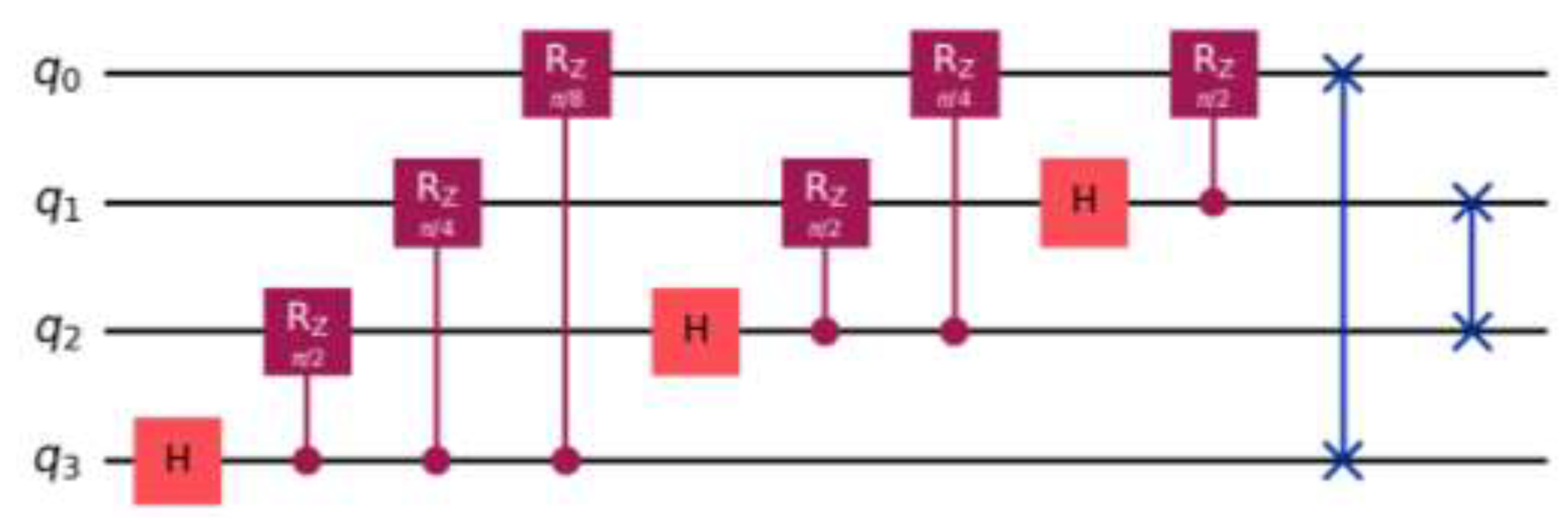
Figure 2.
Quantum circuit schematics for the inverse QFT.
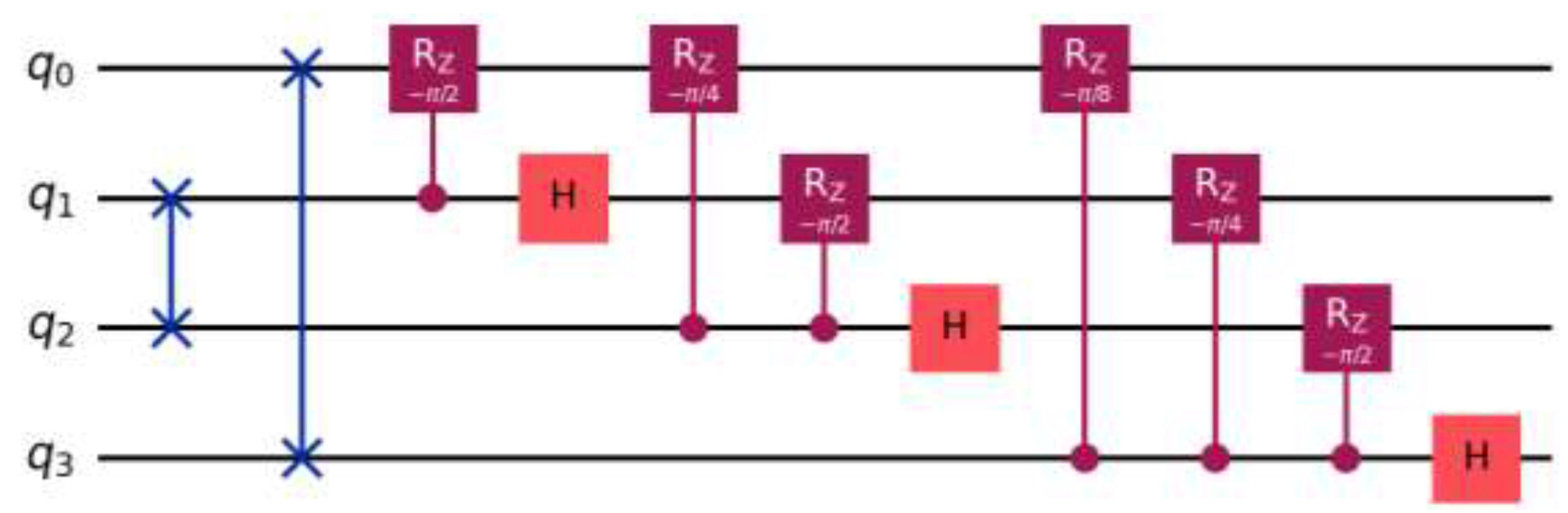
Figure 3.
A generic quantum circuit of the QNTT operation using quantum Gentleman-Sande [51].
Figure 3.
A generic quantum circuit of the QNTT operation using quantum Gentleman-Sande [51].
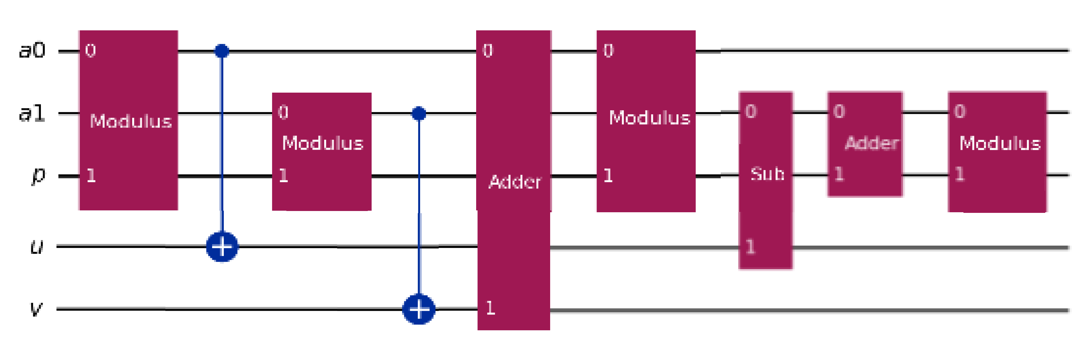
Figure 4.
The quantum circuit for order finding in Shor’s algorithm. Shor-baseline benchmark includes the controlled modular exponentiation block to reflect realistic order-finding depth and noise accumulation on NISQ devices.
Figure 4.
The quantum circuit for order finding in Shor’s algorithm. Shor-baseline benchmark includes the controlled modular exponentiation block to reflect realistic order-finding depth and noise accumulation on NISQ devices.
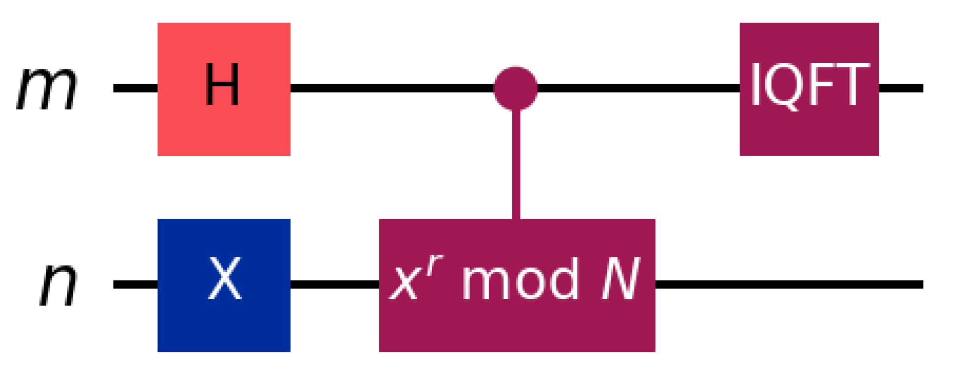
Figure 5.
The proposed new hybrid classical-quantum JVG algorithm for number factorization. The modular exponentiation is computed on a classical device. The information is later mapped into Hilbert space so it can be processed within a quantum framework for the JVG quantum circuit.
Figure 5.
The proposed new hybrid classical-quantum JVG algorithm for number factorization. The modular exponentiation is computed on a classical device. The information is later mapped into Hilbert space so it can be processed within a quantum framework for the JVG quantum circuit.
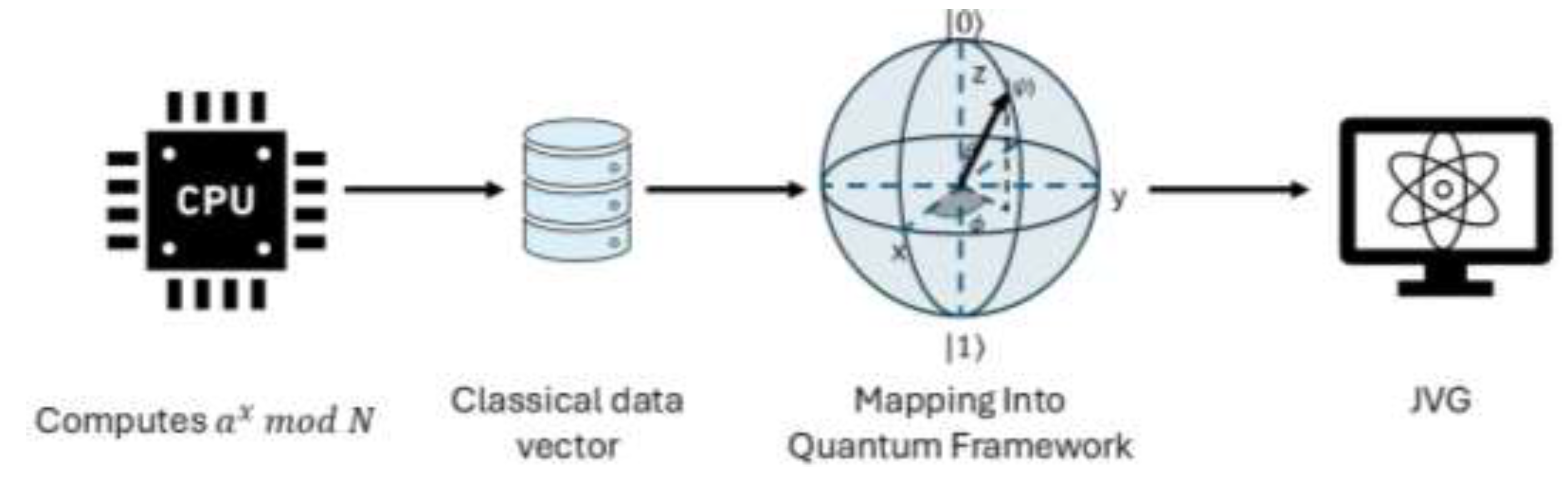
Figure 6.
The proposed new quantum circuit for number factorization using QNTT. Note that the qubits are encoded as amplitudes before being processed by the IQNTT circuit.
Figure 6.
The proposed new quantum circuit for number factorization using QNTT. Note that the qubits are encoded as amplitudes before being processed by the IQNTT circuit.
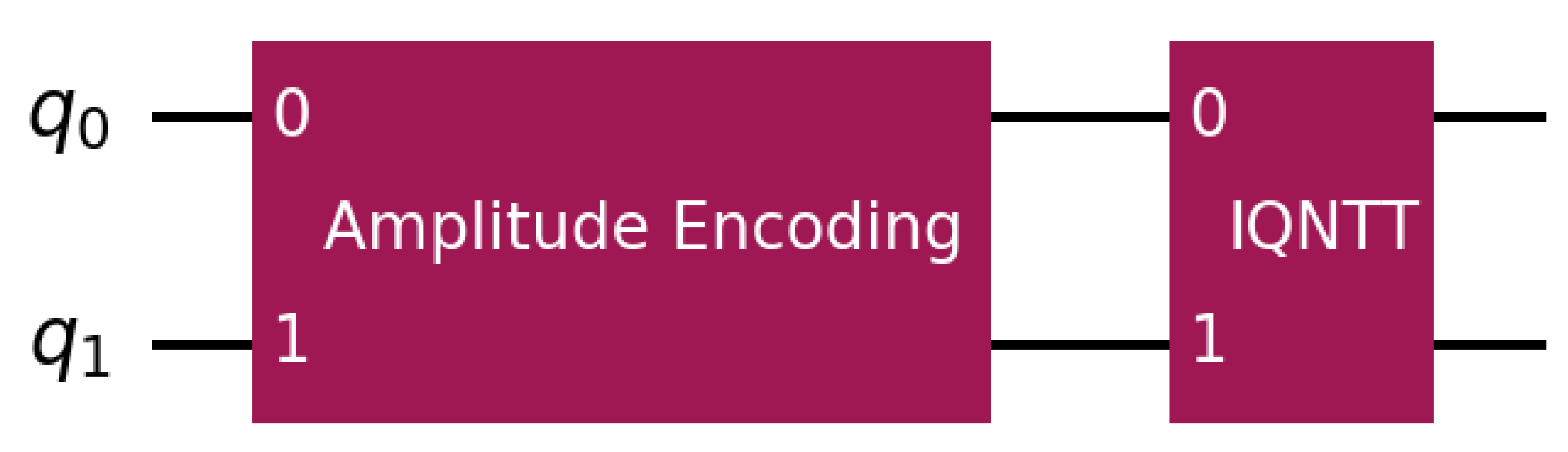
Figure 7.
Plot for the simulated growth-rates for running time on a Log10 scale.
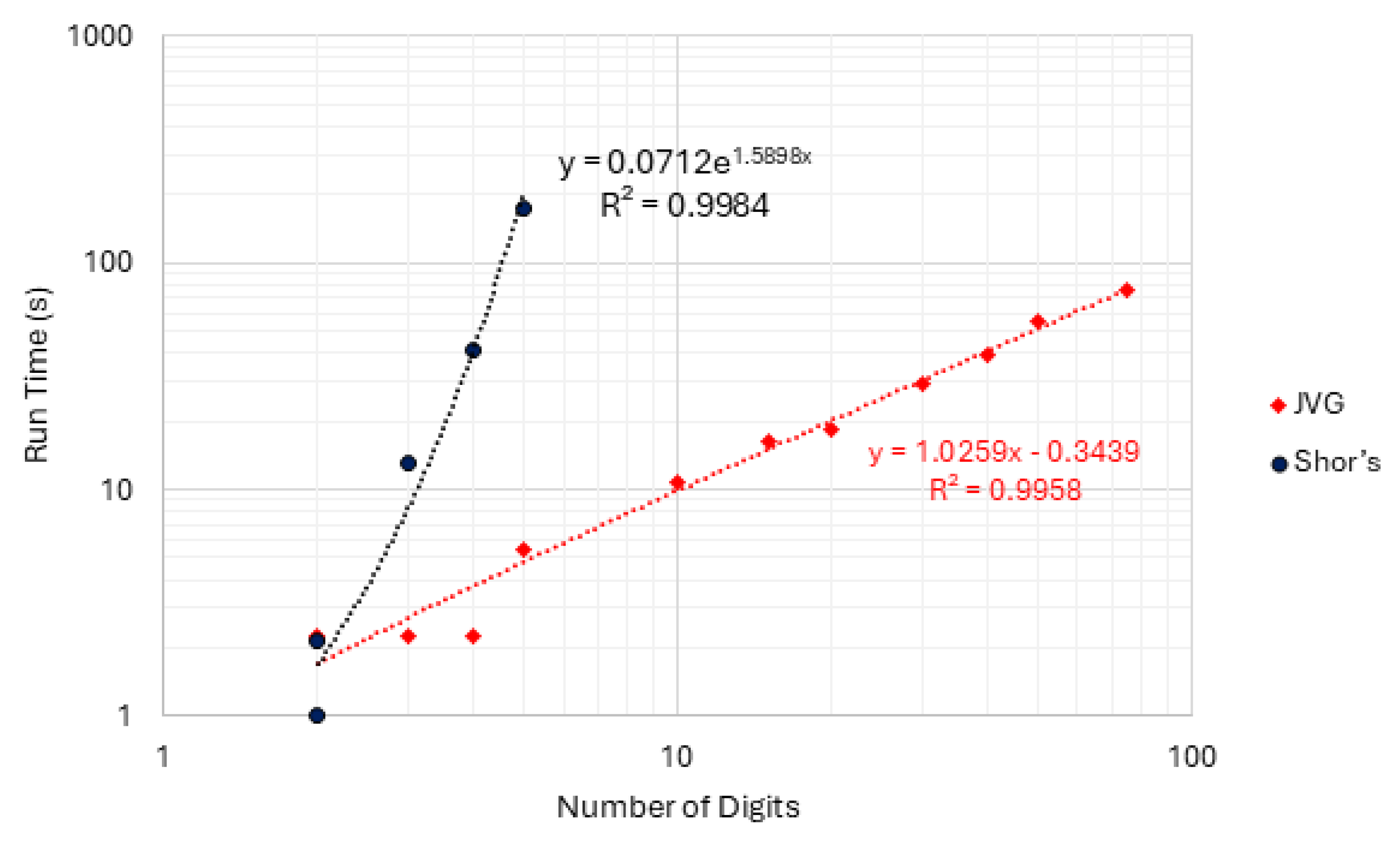
Figure 8.
Plot for the simulated growth-rates for RAM on a Log10 scale.
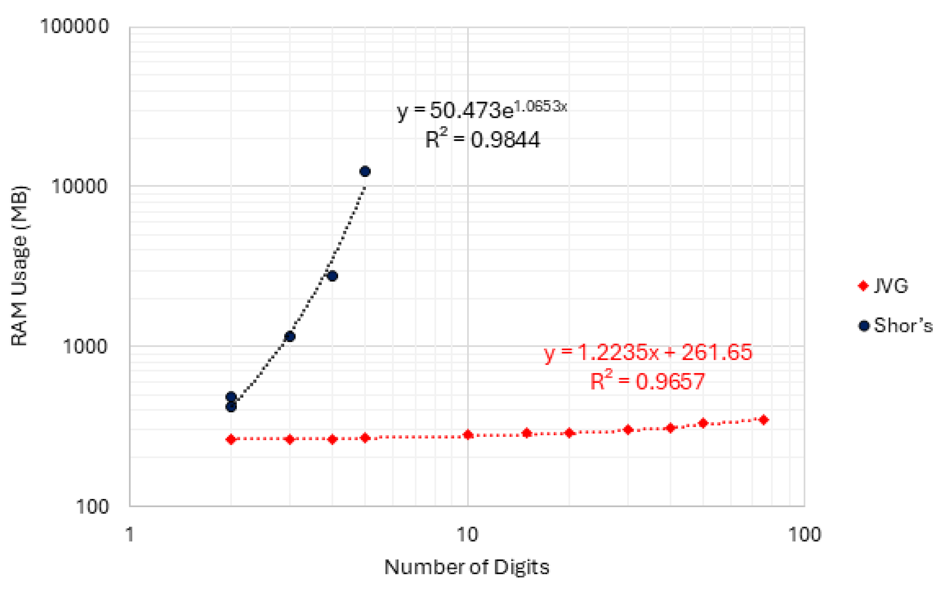
Figure 9.
Plot for the experimental growth-rates for Qiskit Runtime, on a Log10 scale.
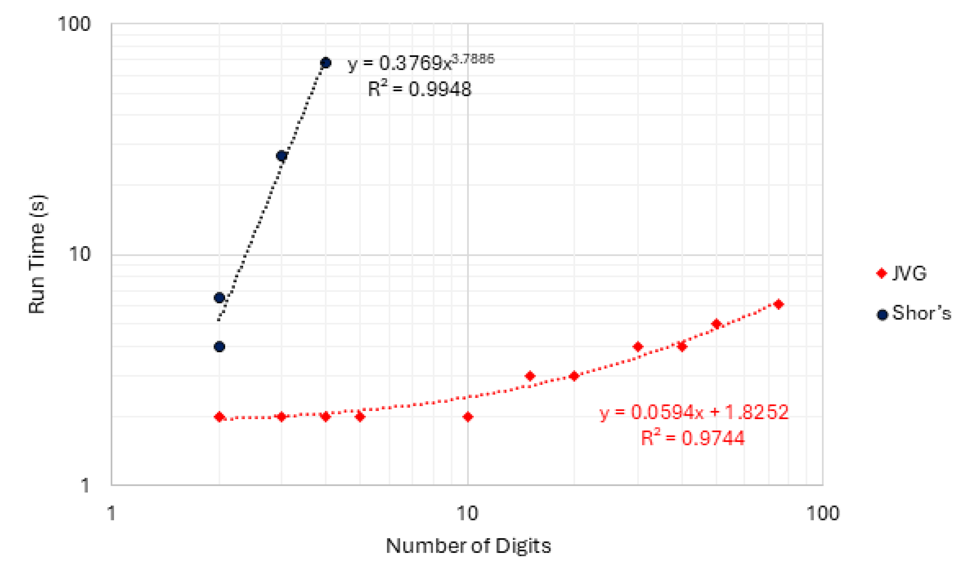

Table 1.
Hardware for the quantum simulations using a classical computer.
| RAM (GB) | CPU | GPU |
|---|---|---|
| 32 | 13th Generation i7 | RTX 4080 16 GB |
Table 2.
Composite numbers evaluated.
| Number of Digits |
Tested Using Shor’s Algorithm | Tested Using JVG’s Algorithm |
|---|---|---|
| 2 | Solved | Solved |
| 3 | Solved | Solved |
| 4 | Solved | Solved |
| 5 | Solved | Solved |
| 10 | Not Capable | Solved |
| 15 | Not Capable | Solved |
| 20 | Not Capable | Solved |
| 30 | Not Capable | Solved |
| 40 | Not Capable | Solved |
| 50 | Not Capable | Solved |
| 75 | Not Capable | Solved |
Table 3.
Results for the simulations of number factorization for both algorithms.
| Algorithm | Number of digits (qubits) | Run Time (s) |
RAM Usage (MB) |
CX | U | ||||
|---|---|---|---|---|---|---|---|---|---|
| Shor’s | 2 (18) | 1.01 ± 0.01 | 419 ± 1.22 | 10541 ± 7 | 13971 ± 10 | ||||
| JVG | 2 (6) | 2.20 ± 0.27 | 261 ± 2.46 | 552 ± 0 | 657 ± 0 | ||||
| Shor’s | 2 (22) | 2.15 ± 0.02 | 488 ± 7.61 | 21840 ± 6 | 29448 ± 18 | ||||
| JVG | 2 (6) | 2.26 ± 0.05 | 260 ± 0.38 | 552 ± 0 | 657 ± 0 | ||||
| Shor’s | 3 (34) | 13.16 ± 0.13 | 1159 ± 10.30 | 109994 ± 9 | 153827 ± 40 | ||||
| JVG | 3 (6) | 2.26 ± 0.05 | 261 ± 0.5 | 552 ± 0 | 657 ± 0 | ||||
| Shor’s | 4 (46) | 40.91 ± 0.63 | 2794 ± 26.30 | 344116 ± 12 | 490193 ± 42 | ||||
| JVG | 4 (6) | 2.24 ± 0.06 | 260 ± 0.66 | 552 ± 0 | 657 ± 0 | ||||
| Shor’s | 5 (70) | 174.11 ± 2.40 | 12505 ± 297.68 | 1713476 ± 16 | 2485724 ± 130 | ||||
| JVG | 5 (10) | 5.48 ± 0.14 | 267 ± 0.66 | 1720 ± 0 | 1975 ± 0 | ||||
| Shor’s | - | - | - | - | - | ||||
| JVG | 10 (16) | 10.70 ± 0.31 | 278 ± 0.72 | 3475 ± 0 | 3962 ± 2 | ||||
| Shor’s | - | - | - | - | - | ||||
| JVG | 15 (22) | 16.43 ± 0.56 | 289 ± 0.59 | 5238 ± 0 | 5958 ± 1 | ||||
| Shor’s | - | - | - | - | - | ||||
| JVG | 20 (24) | 18.57 ± 0.83 | 289 ± 2.03 | 5821 ± 0 | 6618 ± 0 | ||||
| Shor’s | - | - | - | - | - | ||||
| JVG | 30 (34) | 28.98 ± 0.90 | 303 ± 3.93 | 8736 ± 0 | 9918 ± 0 | ||||
| Shor’s | - | - | - | - | - | ||||
| JVG | 40 (42) | 39.19 ± 0.92 | 312 ± 1.01 | 11098 ± 0 | 12590 ± 0 | ||||
| Shor’s | - | - | - | - | - | ||||
| JVG | 50 (54) | 54.49 ± 0.98 | 328 ± 3.31 | 14596 ± 0 | 16550 ± 0 | ||||
| Shor’s | - | - | - | - | - | ||||
| JVG | 75 (70) | 75.69 ± 1.46 | 345 ± 1.49 | 19322 ± 0 | 21894 ± 0 | ||||
| Average Coefficient of Variation | Shor’s | 1.17% | 1.21% | 0.02% | 0.03% | ||||
| JVG | 5.53% | 0.50% | 0.00% | 0.00% | |||||
Table 4.
Results for the implementation of number factorization for both algorithms on a real quantum computer.
Table 4.
Results for the implementation of number factorization for both algorithms on a real quantum computer.
| Algorithm | Number of digits (qubits) | QR (s) |
SX | CZ | RZ | ||||
|---|---|---|---|---|---|---|---|---|---|
| Shor’s | 2 (18) | 4.0 ± 0 | 54390 ± 230 | 26444 ± 129 | 24761 ± 142 | ||||
| JVG | 2 (6) | 2.00 ± 0 | 2019 ± 10 | 1023 ± 7 | 1350 ± 4 | ||||
| Shor’s | 2 (22) | 6.5 ± 0.5 | 116626 ± 397 | 56942 ± 210 | 50738 ± 176 | ||||
| JVG | 2 (6) | 2 ± 0 | 2014 ± 3 | 1020 ± 3 | 1351 ± 3 | ||||
| Shor’s | 3 (34) | 26.8 ± 0.9 | 642895 ± 1098 | 314000 ± 536 | 254806 ± 456 | ||||
| JVG | 3 (6) | 2 ± 0 | 2031 ± 3 | 1018 ± 4 | 1333 ± 8 | ||||
| Shor’s | 4 (46) | 67.8 ± 2.5 | 2085030 ± 2554 | 1013958 ± 1468 | 805239 ± 1627 | ||||
| JVG | 4 (6) | 2 ± 0 | 2013 ± 4 | 1019 ± 3 | 1350 ± 4 | ||||
| Shor’s | 5 (70) | - | - | - | - | ||||
| JVG | 5 (10) | 2 ± 0 | 6762 ± 84 | 3387 ± 47 | 4184 ± 21 | ||||
| Shor’s | - | - | - | - | - | ||||
| JVG | 10 (16) | 2 ± 0 | 14423 ± 118 | 7203 ± 61 | 8532 ± 62 | ||||
| Shor’s | - | - | - | - | - | ||||
| JVG | 15 (22) | 3 ± 0 | 22541 ± 255 | 11283 ± 129 | 12952 ± 62 | ||||
| Shor’s | - | - | - | - | - | ||||
| JVG | 20 (24) | 3 ± 0 | 25282 ± 197 | 12652 ± 97 | 14338 ± 75 | ||||
| Shor’s | - | - | - | - | - | ||||
| JVG | 30 (34) | 4 ± 0 | 39313 ± 228 | 19688 ± 150 | 21598 ± 69 | ||||
| Shor’s | - | - | - | - | - | ||||
| JVG | 40 (42) | 4 ± 0 | 50762 ± 355 | 25416 ± 170 | 27469 ± 97 | ||||
| Shor’s | - | - | - | - | - | ||||
| JVG | 50 (54) | 5 ± 0 | 68143 ± 1138 | 34134 ± 587 | 36130 ± 61 | ||||
| Shor’s | - | - | - | - | - | ||||
| JVG | 75 (70) | 6.1 ± 0.32 | 91734 ± 771 | 45951 ± 397 | 47823 ± 111 | ||||
| Average Coefficient of Variation | Shor’s | 3.80% | 0.26% | 0.29% | 0.33% | ||||
| JVG | 0.43% | 0.73% | 0.82% | 0.39% | |||||
Note: QR (s) denotes Qiskit Runtime wall-clock time reported by the runtime service.
Disclaimer/Publisher’s Note: The statements, opinions and data contained in all publications are solely those of the individual author(s) and contributor(s) and not of MDPI and/or the editor(s). MDPI and/or the editor(s) disclaim responsibility for any injury to people or property resulting from any ideas, methods, instructions or products referred to in the content. |
© 2026 by the authors. Licensee MDPI, Basel, Switzerland. This article is an open access article distributed under the terms and conditions of the Creative Commons Attribution (CC BY) license (http://creativecommons.org/licenses/by/4.0/).
Copyright: This open access article is published under a Creative Commons CC BY 4.0 license, which permit the free download, distribution, and reuse, provided that the author and preprint are cited in any reuse.


