1. Introduction
The introduction should provide a brief overview of the study's context and highlight its significance. It should define the purpose of the work and its importance. The current state of the research field should be carefully reviewed, and key publications should be cited. Please highlight controversial and diverging hypotheses when necessary. Finally, briefly mention the main aim of the work and highlight the principal conclusions. To the extent possible, please keep the introduction comprehensible to scientists outside your specific field of research. References should be numbered in order of appearance and indicated by a numeral or numerals in square brackets—e.g., [
1] or [
2,
3], or [
4,
5,
6]. See the end of the document for further details on references.
1.1. Development of Predictive Models
The basic model for predicting the draught forces acting on tillage tools assumes that the tool cutting through the soil creates a soil wedge, leading to the displacement of the cut soil pile [
1]. Söhne's model is widely regarded as a pioneering approach, enabling scientists to predict forces using the basic principles of soil mechanics. The model assumes that the soil behaves rigidly and requires several simplistic assumptions, such as soil homogeneity and constant contact conditions between the soil and the tool. The model validates well for narrow tools, but is less effective for wide tools with complex geometries.
The theoretical foundations of draught force prediction developed by Söhne were created by integrating more detailed parameters related to tool geometry, such as the cutting edge angle of the tool and soil consistency [
2]. McKyes' model is commonly used to predict the forces acting on wide tools. McKyes' model is one of the most widely accepted in agricultural engineering due to its versatility for predicting horizontal forces acting on tools. However, the model's assumptions are adapted to narrow tools with straight edges, which limits its direct application to tools such as duckfoot.
Another improved model of soil-tool interaction considers both draught and vertical forces, providing a more comprehensive understanding of tool behaviour in different soil conditions [
3]. This model highlights the importance of soil parameters, including moisture content and bulk density, as well as the influence of soil adhesion and cohesion on tool resistance. However, like the Söhne and McKyes models, the Perumpral model has been limited due to its application to tools with simpler geometries and narrow cutting edges.
Until the end of the 90s of the twentieth century, most of the analysed models were two-dimensional, which explained the operation of wide tools [
1,
4,
5]. Based on the assumption that the cross-section of the plane parallel to the direction of motion of the surface separating the detached soil from the monolith is a logarithmic spiral [
6], a system of equations of force equilibrium acting on a deformed soil block was developed, the vertical cross-section of which is represented in the form of a connection between a logarithmic spiral and a straight line [
7]. Based on this theory, Reece [
8] developed a universal equation (Eq. 1), which describes the specific force of the tool's pressure on the soil, as detailed in the publication by Hettiaratchi, Witney, and Reece [
9].
where:
F1 – specific force of the tool pressure on the soil, converted to working width, N·m
–1;
γ – volumetric weight of the soil, N·m
–3;
d – depth of tool work, m;
c – cohesion, N·m
–2;
ca – adhesion of the soil to the surface of the tool, N·m
–2;
q – external pressure exerted on the soil surface, N·m
–2;
Nγ,
Nc,
Nca,
Nq – dimensionless coefficients determined experimentally, read from graphs for different tool rake angles and angles of internal friction of the soil and external soil-tool.
Four expressions in the model (Eq. 1) represent, in order, the gravitational, cohesive, adhesive, and additional (from the embankment) components of the soil reaction, without taking into account the forces of inertia, due to the relatively small deformations of the soil. Therefore, the influence of the speed of tool movement was omitted. From studies carried out in cohesive and frictional soils, it has been confirmed that the effects of inertia on the traction force for tine are not significant below the speed
and are limited to the speed
, where
g is the acceleration in m·s
–2,
w is the width of the tool in m, and
d is the depth of tool work in m [
10]. It was also found that the effects of the tool's speed of movement are less significant compared to its working depth [
11].
The cited model (Eq. 1) is a slight extension of the Terzaghi equation [
5], to which an expression with adhesion resistance has been added. Because soil-tool adhesion has little effect on specific force
F1, its authors combined the expressions of adhesion with cohesion, introducing the concept of conjugated adhesion [
9], thus returning to the Terzaghi equation [
5], Eq. 2.
where:
F1 – specific force of the tool pressure on the soil, converted to working width, N·m
–1;
γ – volumetric weight of the soil, N·m
–3;
d – depth of tool work, m;
c – cohesion, N·m
–2;
q – external pressure exerted on the soil surface, N·m
–2;
Nγ,
Nc,
Nq – dimensionless coefficients.
In McKyes' fundamental textbook [
2], the analysed model (Eq. 1) is represented by the tool's force on the soil (Eq. 3), which was obtained by multiplying Eq. 1 by the tool width
w, and the components of the force were determined: draught (horizontal) (Eq. 4) and vertical (Eq. 5).
where:
F – resultant force of the tool's pressure on the soil, N;
γ – volumetric weight of the soil, N·m
–3;
d – depth of tool work, m;
c – cohesion, N·m
–2;
ca – adhesion of the soil to the surface of the tool, N·m
–2;
q – external pressure exerted on the soil surface, N·m
–2;
w – width of the tool, m;
Nγ,
Nc,
Nca,
Nq – dimensionless coefficients;
Fx – draught force, component of horizontal force, N;
α – angle of the tool, °;
δ – angle of external friction soil-steel, °;
Fy – component of vertical force, N.
The universal equation of soil motion was used to analyse the work of the subsoiler's tine with the wings, and it was found that the results did not always correlate well with the experimental values for different rake angles of the wings [
12].
In developing the model under consideration (Eq. 1), the slip lines in the soil were determined [
9], and the mechanical determinants of agricultural soil deformation were presented [
13]. Thought experiments were conducted, confirmed by empirical research, and a model (Eq. 6) was developed to optimise the working conditions of tools in terms of energy [
14].
where:
E' – specific energy needed to deform the soil, J·m
–3;
d – depth of tool work, m;
w – working width of the tool, m;
γ – volumetric weight of the soil, N·m
–3;
v – speed of tool movement, m·s
–1;
ka,
k',
k – empirical coefficients.
In the discussed models, it was assumed that the tool moves in progressive motion in different directions relative to the level, without considering the momentary oscillations of forces and the cross-section of the loosened soil.
1.2. Wide Tools and Challenges in Duckfoot Modelling
Duckfoots, known for their wide, triangular blades, pose a unique challenge because their wing geometry significantly affects the distribution of forces. Current models, such as those by Söhne, McKyes, and Perumpral, do not consider such geometries or complex soil-tool interactions with work elements that have large side spans of cutting edges, particularly in relation to the working depth. These models assume a relatively simple geometry, with straight or slightly curved blades that cannot capture the complex interaction between the duckfoots wide wings and the soil. The lateral displacement caused by duckfoot wings requires modification of existing models to accommodate different shear and cracking patterns in the soil. These models do not account for changes in soil strength, moisture content, and cohesion, which can dynamically change during fieldwork. This gap is particularly pronounced in compacted soils, where these variables fluctuate significantly.
Empirical studies on duckfoots show that their interaction with the soil differs from that of narrow tools, due to their wide cutting edges and ability to work efficiently at shallow depths. The forces acting on these tools depend highly on soil properties such as moisture content, density, and the elastic properties of the tines to which the duckfoots are attached. Therefore, using models developed for narrow chisel tools is impossible without significant modifications.
Given the limitations of existing models for predicting forces acting on duckfoots, there is a clear need to modify and adapt the Söhne, McKyes, and Perumpral models to more accurately reflect the actual operating conditions of these wide tools. In particular, it is necessary to create modified models that account for the unique geometry of the duckfoot, which results in significant vertical and lateral displacement of the soil, while considering soil properties and operating conditions.
The study's primary goal is to modify the Söhne, McKyes, and Perumpral models to enable more accurate prediction of the draught force acting on the duckfoot. These modifications are designed to eliminate the limitations of current models, particularly in relation to wide tools and the impact of soil properties. The modified models will be validated with empirical data collected from laboratory experiments to confirm their effectiveness.
Based on these considerations, explanatory hypotheses were formulated: H1: Modification of the Söhne, McKyes, and Perumpral models to include the unique duckfoot geometry will significantly improve the accuracy of draught force prediction; H2: The modified models, experimentally verified, will allow for reliable and stable predictions of traction force under different operating conditions, taking into account variability in soil moisture content and compaction.
The novelty of this article lies in the modification of established models (Söhne, McKyes, and Perumpral) to predict the draught force for wide tools, such as duckfoots. While these models have been widely used for narrow tools with simple shapes, their use for wide tools has been limited. This paper presents innovative solutions in the first adaptation of these three models for duckfoot, which has a significantly different geometry than the tools for which these models were initially developed. These creative modifications of the models aim to fill a significant gap in the current knowledge of models that consider soil-tool interactions by adapting existing theoretical frameworks to duckfoots. This will allow for improved design and optimisation of tools in agricultural engineering.
2. Theoretical Model of Duckfoot Work in Soil
2.1. General Data and Assumptions
The analysis was carried out in a 2
D system, excluding lateral deformations relative to the cutting edge of the duckfoot. Since the throw from the top of the knife resembles two elements connected in a triangle, the calculations were made for one side perpendicular to the edge. The results were then doubled, and after rotating the X
oY
oZ
o system by the angle of the duckfoot wing, the components of the forces in the XYZ system were determined (
Figure 1). The structural model took into account the shape and dimensions of the deformed soil pile and soil–duckfoot forces, using the laws and theorems of mechanics.
The same assumptions were introduced when modifying mathematical models: 1. The soil is homogeneous and isotropic; 2. Deformation is considered in 2D (tool width > tool working depth); 3. Soil cracking meets the Coulomb-Mohr criterion; 4. Soil parameters: bulk density (volumetric weight), angle of internal friction (soil-soil), angle of external friction (soil-steel), cohesion, and adhesion depend only on soil moisture content; 5. The width of the soil pile is equal to the length of the blade edge; 6. The cutting resistance of the blade's sharp edge is omitted; 7. Duckfoot operates at a constant depth, and the angles of setting and clearance remain unchanged, despite the use of elastic tines. 8. The movement of the tool is uniform.
The mathematical models were modified to a 2D space and duckfoot geometry, and the existing designations were considered [
15] to ensure consistency in deliberations and analysis.
2.2. Model 1 Söhne
The soil cracking pattern for model 1 Söhne in 2
D space assumes stepped cracking of the soil as shown in
Figure 1. Model 1 for 2
D was presented by Söhne [
1,
1] and modified by Rowe and Barnes [
16]. The coupled forces in the soil-tool system include the weight of the soil pile (soil wedge)
G, the cohesion force at the surface of soil cracking due to soil pile shear
Fc, the standard component of the soil reaction on the fracture surface
Nf, the tangential component of the soil reaction at the fracture surface
Tf =
μfNf, adhesion force at the soil-duckfoot boundary
Fca, a normal component of soil surface reaction
Ns, the tangential component of the soil response to duckfoot
Ts =
μsNs, inertia force
Fa, vertical force
Fy and draught
Fx. Soil-steel friction coefficient
μs is equal to tan
δ, where
δ is the angle of external friction of soil-steel, while the coefficient of friction of soil-soil pile
μf is equal to tan
φ, where
φ is the angle of internal friction of the soil.
After adding the horizontal and vertical forces and comparing them to zero, and eliminating the reaction components
Nf and
Ns obtained by the horizontal component, which is the draught force for duckfoot [
17], Eq. 7, and the vertical component of duckfoot pressure on the soil, Eq. 8.
where Z is the auxiliary variable described by Eq. 9.
where:
Fx – draught force, N;
Fy – vertical component of the pressure force of the duckfoot on the soil, N;
G – weight of the soil pile, N;
Z – auxiliary variable;
c – cohesion, N·m
–2;
Af – shear area of the soil pile, m
2;
Fa – inertia force of the soil pile, N;
ca – adhesion of the soil to the surface of the tool, N·m
–2,
Aw – area of the surface of the soil pile on the duckfoot wing, m
2;
α – duckfoot wing angle, °;
β – soil shear angle, °;
δ – angle of external friction soil-steel, °;
φ – angle of internal friction of the soil, °;
θo – lateral angle of the duckfoot wing, °.
Other variables found in the Eqs. 7–9 were designated with the Eqs. 10–13.
where:
G – weight of the soil pile, N;
γ – volumetric weight of the soil, N·m
–3;
ls – duckfoot blade length, m;
ww – wing width of duckfoot, m;
α – duckfoot wing angle, °;
β – soil shear angle, °;
φ – angle of internal friction of the soil, °;
Fa – inertia force of the soil pile, N;
d – depth of work duckfoot, m;
v – speed of tool movement, m·s
–1;
g – acceleration of gravity, m·s
–2;
Aw – area of the soil pile on the duckfoot wing, m
2;
Af – shear area of the soil pile, m
2.
After the modification, the Söhne's model has been adapted to the specifics of duckfoot work, providing a better description of the actual direction of soil movement and its dynamic interaction with the tool. It takes into account the lateral angle of application of the wings, the weight of the soil wedge, cohesion, adhesion, internal and external friction, and components of the soil reaction.
2.3. Model 2 McKyes
The geometry of the soil pile in model 2 is in the shape of a soil wedge, which is attributed to McKyes [
2,
18]. For 2
D spaces and wide tools, it consists only of a central part, a flat wedge inclined at an angle α for the tool position and sliding on the soil surface at a shear angle
β. The interaction of the forces related to the action of the duckfoot on the soil involves the weight of the soil wedge G, soil reaction
Nf, cohesion
c, adhesion
ca, and specific cutting force
F1. Specific cutting force
F1 is the force per unit length of the blade and is given in the form of the universal equation of soil motion, Eq. 1 [
8].
As mentioned, the specific cutting force
F1 can be multiplied by the width of the duckfoot
w, considering the lateral angle of the duckfoot wing
θo. In this way, the resultant pressure force of the duckfoot on the soil is obtained, with a dynamic expression that considers the speed of soil movement on the wings of the duckfoot, but without external pressure on the soil surface
q, Eq. 14.
where:
F – resultant force of the tool's pressure on the soil, N;
γ – volumetric weight of the soil, N·m
–3;
d – depth of work duckfoot, m;
w – width of duckfoot, m;
c – cohesion, N·m
–2;
ca – adhesion of the soil to the surface of the tool, N·m
–2;
v – speed of tool movement, m·s
–1;
g – acceleration of the earth, m·s
–2;
Nγ,
Nc,
Nca,
Na – dimensionless coefficients;
θo – lateral angle of the duckfoot wing, °.
Dimensionless coefficients, related to the weight of the soil pile
Nγ, soil cohesion
Nc, soil-duckfoot adhesion
Nca, and the inertia of the soil pile
Na, were assigned with the Eqs. 15–18 [
17].
where:
Nγ,
Nc,
Nca,
Na – dimensionless coefficients;
d – depth of work duckfoot, m;
r – extent of the soil pile cracking, m;
α – duckfoot wing angle, °;
β – soil shear angle, °;
δ – angle of external friction soil-steel, °;
φ – angle of internal friction of the soil, °.
The breakage range of the soil pile was determined from Eq. 19.
where:
r – range of cracking of the soil pile, m;
d – depth of work duckfoot, m;
α – duckfoot wing angle, °;
β – soil shear angle, °.
The draught force and vertical component of the duckfoot pressure on the soil were obtained by combining the resultant contact force with the adhesion force, Eqs. 20 and 21, respectively.
where:
Fx – draught force, horizontal component of the pressure force of duckfoot on the soil, N;
Fy – vertical component of the pressure force of the duckfoot on the soil, N;
F – resultant pressure force of the duckfoot on the soil, N;
ca – adhesion of the soil to the surface of the tool, N·m
–2,
ww – width of the duckfoot wing, m;
ls – duckfoot blade length, m;
α – duckfoot wing angle, °;
δ – angle of external friction soil-steel, °;
θo – lateral angle of the duckfoot wing, °.
After modification, McKyes' model 2 was adapted to work with duckfoots by introducing a lateral angle of application θo and taking into account the dynamic influence of the speed of soil movement along the wings of the tool. The model describes the soil wedge as a flat wedge sliding on the soil surface at an angle of shear β. In the balance of forces, it takes into account the weight of the pile, cohesion, adhesion, friction, and the inertia force, incorporating the sin2θo factor. As a result, it allows for the determination of the resultant pressure force on the soil and its distribution into the draught force Fx and the vertical component Fy, better reflecting the real working conditions of wide duckfoot tools.
2.4. Model 3 Perumpral
Model 3, presented by Swick and Perumpral [
3], assumes the same soil fracture wedge and force system as model 2 by McKyes. Analysing the balance of forces acting on the middle soil wedge gave expressions for the resultant soil cutting force by duckfoot
F, Eq. 22.
where:
F – resultant force of the tool's pressure on the soil, N;
Fc – cohesion force on the soil shear surface, N;
Fca – adhesion force at the contact surface of the soil pile with the duckfoot wing, N;
G – weight of the soil pile, N;
Fa – inertia force of the soil pile, N;
α – duckfoot wing angle, °;
β – soil shear angle, °;
δ – angle of external friction soil-steel, °;
φ – angle of internal friction of the soil, °;
θo – lateral angle of the duckfoot wing, °.
The other variables were calculated from the Eqs. 23–27.
where:
Fc – cohesion force on the soil shear surface, N;
Fca – adhesion force at the contact surface of the soil pile with the duckfoot wing, N;
G – weight of the soil pile, N;
Fa – inertia force of the soil pile, N;
r – extent of the soil pile cracking, m;
ca – adhesion of the soil to the surface of the tool, N·m
–2,
c – cohesion, N·m
–2;
ls – duckfoot blade length, m;
ww – wing width of duckfoot, m;
d – depth of work duckfoot, m;
γ – volumetric weight of the soil, N·m
–3;
v – speed of tool movement, m·s
–1;
g – acceleration of gravity, m·s
–2;
α – duckfoot wing angle, °;
β – soil shear angle, °.
The draught force and vertical component of the duckfoot pressure on the soil were obtained, as given in model 2, by combining the resultant contact force with the adhesion force, Eqs. 28 and 29, respectively, which were rewritten to create the complete algorithm.
where:
Fx – draught force, horizontal component of the pressure force of duckfoot on the soil, N;
Fy – vertical component of the pressure force of the duckfoot on the soil, N;
F – resultant pressure force of the duckfoot on the soil, N;
ca – adhesion of the soil to the surface of the tool, N·m
–2,
ww – width of the duckfoot wing, m;
ls – duckfoot blade length, m;
α – duckfoot wing angle, °;
δ – angle of external friction soil-steel, °;
θo – lateral angle of the duckfoot wing, °.
In the modified model 3 of Perumpral, the wedge geometry and the system of forces, similar to the McKyes model, were retained. Still, the equilibrium equations were developed to determine the cutting force of the soil directly.
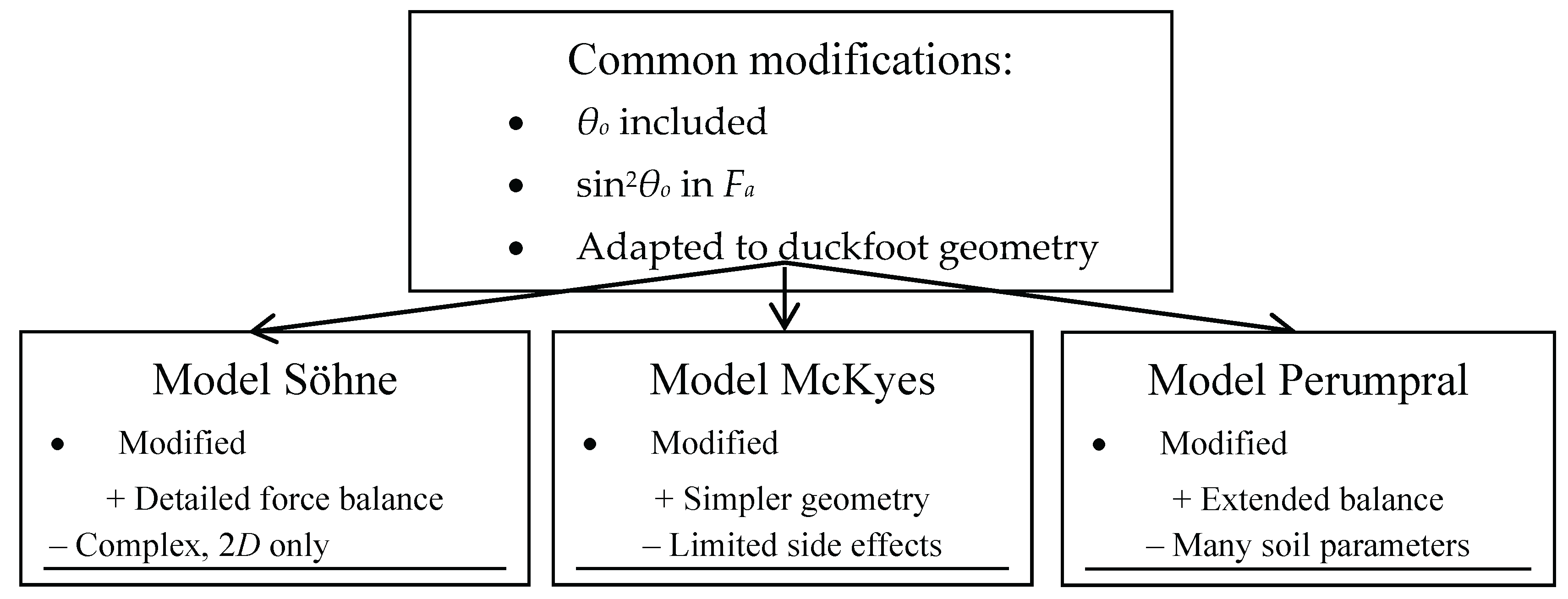
In the summary of the changes, a comparative diagram of the three modified analytical models for duckfoots (Söhne, McKyes, Perumpral) is provided,
Figure 2, which illustrates the common modifications and the advantages and limitations of each approach.
The mathematical models were validated for the draught force Fx using experimental data for the same technical parameters.
3. Materials and Methods
3.1. Soil Properties
Soil bin tests were conducted at the Department of Biosystems Engineering, Institute of Mechanical Engineering, Warsaw University of Life Sciences, to obtain data for verifying the analytical model. The soil bin was filled with light loamy sand, comprising clay, silt, and sand fractions of 2%, 36%, and 62%, respectively, as determined by the sieve separation method. The dry soil volume density was 1535 ± 11 kg·m⁻³, and the compaction of 486 ± 25 kPa was determined using a 30° cone penetrometer with a base diameter of 20.27 mm, in accordance with the ASAE S 313.2 standard [
19]. The drying-weighing method determined soil moisture contents of 10% and 14% (wet basis), in accordance with the ISO 11465 standard [
20].
For both moisture contents, the mechanical properties of the soil were investigated in the annular rotary Schulze shear apparatus at the Institute of Agrophysics of the Polish Academy of Sciences in Lublin [
21]. The soil was pre-consolidated at pressures of 10, 20, 30, 40, and 50 kPa [
22]. For moisture content levels of 10% and 14%, the values of the angle of internal friction were 37° and 32°, respectively. The values of the angle of friction for soil-steel were 24° and 22°, respectively. The cohesion was 17 kPa and 18 kPa, and adhesion was 10 kPa and 12 kPa, respectively. The index of flowability,
ffc, was 1.50 and 1.60, respectively. According to the classification [
23], this soil was classified as a cohesive material, because the value of
ffc was within the range of 1 <
ffc < 2.
3.2. Test Objects
Three duckfoots with widths of 105, 133, and 202 mm, labeled A105, B135, and C200, were used in the study. Duckfoot was attached to S-type and VCO-type tines, with stiffnesses of 5.3 kN·m⁻¹ and 8.3 kN·m⁻¹, respectively. Although the shape and characteristic angles of duckfoots were similar, when combined with the S and VCO tines, the landing angles were 8° and 2°, respectively [
24].
3.3. Soil Bin with Measuring Equipment
The tine with a duckfoot was attached to the frame of a tool trolley pulled by a rope system driven by a 22.0 kW WAR 1M4 TF electric motor, coupled to a FUA 85A 16 1M4 TF gearbox. The rotational speed was determined by a V2500-0220 TFW1 inverter (Watt Drive, Austria). The trolley's movement speed with working elements was monitored by an optical sensor (CS3D, ZEPWN, Marki, Poland). The depth of duckfoot work was determined and controlled using a laser distance meter (LDS 100-500P-S, Beta Sensorik) combined with a 3000 mm horizontal displacement indicator, with a sensitivity of 0.3163 mV V⁻¹ mm⁻¹ (WS12-3000-R1K-L10-M, ASM GmbH, Germany). The measurement data were recorded on a computer via a high-speed digital interface board from Hottinger Baldwin, specifically the DMCplus. The measurement and control system was controlled by the CATMAN 2.1 software, which provided simultaneous data acquisition and motion control, with a sampling rate of 50 Hz.
3.4. Measurement Procedure
The soil at a depth of 0.6 m was loosened with tines using a subsoiler to a depth of 0.22 ± 0.02 m, levelled with a scraper, and compacted with a roller weighing 360–520 kg, according to a verified procedure [
24]. The research was conducted at three duckfoot working depths: 30, 50, and 70 mm, and at three movement speeds: 0.84, 1.67, and 2.31 m·s⁻¹. These variables were combined into a factorial experiment with the following design: 3 × 2 × 3 × 3 × 2 (duckfoot width × tine × working depth × movement speed × soil moisture content, respectively), with three or four blocks (replications).
3.5. Statistical Analysis
Separately, for soil moisture contents of 10% and 14%, the optimal values of internal
φ and external
δ friction angles and soil shear
β were determined, using the method of minimising differences between empirical values of traction force (
Fxe) and values calculated from theoretical models (
Fxp), Eq. 30 and using the open-source Python software's v. 3.11.5 (
https://www.python.org).
where:
Fxei –
ith empirical value of the draught force, N;
Fxpi(
φ,
δ,
β) –
ith value of the force calculated from the model at given angles, N; N – number of observations
Based on the minimisation of this function (Eq. 30), a set of angle values (
φ,
δ,
β) was determined that reproduces the experimental data the best. The L-BFGS-B algorithm was used for optimisation, which allows the constraints for individual angles to be considered. The boundaries were adopted in accordance with the literature data:
φ ∈ [30°, 40°],
δ ∈ [20°, 30°],
β ∈ [27°, 45°] [
2,
25,
26].
The fit of analytical models to the empirical data was assessed based on the mean squared error
RMSE, Eq. 31, mean relative error Eq. 32 and global error Eq. 33.
where:
RMSE – mean squared error, N;
δr – relative match error, %;
δg – global model error, %;
Fxei –
ith experimental value of the draught force, N;
Fxpi –
ith value calculated from the predictive model, N;
N – number of observations in a given case (whole – values for all data; soil moisture contents of 10% and 14%; tine S and VCO; duckfoot A105, B135 and C200; duckfoot working depth 0.030 m, 0.050 m and 0.070 m; tool movement speed 0.84 m·s
–1, 1.67 m·s
–1 and 2.31 m·s
–1).
Selected error rates allow for a comprehensive evaluation of the model. Mean squared error RMSE measures the average magnitude of the deviation of the values calculated from the model from the experimental values, expressed in units of the analysed value, in this case, in Newtons. This error allows for direct physical interpretation, indicating how much the model differs from the measurement data on average. RMSE is sensitive to large deviations because Eq. 31 errors are squared, so it works exceptionally well when evaluating models for outliers and significant local differences.
The advantage of the mean relative error δr is that it takes both positive and negative values, which allows for the identification of the direction of deviation of the model. A positive value indicates an underestimation, while a negative value indicates an overestimation of the model relative to experimental data. Thanks to this, the relative error analysis provides information about the size of the error and its nature.
The global error δg is a normalised version of the mean squared error and is a measure of the total deviation of the model from the experimental values. This indicator enables the evaluation of the overall precision of the model fit, regardless of the units of measurement and the scale of the draught force value.
All three error rates were calculated for the entire dataset and separately for different test conditions (soil moisture content, tine type, duckfoot width, duckfoot working depth, tool movement speed) to compare error values and assess under which conditions the models perform the best. The analysis aimed to obtain the smallest possible error values of RMSE, δr (in absolute terms), and δg, which would indicate high accuracy of the model and its good compatibility with experimental data. The evaluated models should have the lowest values of these error rates.
4. Research Results and Discussion
Analysis of the results for the modified Söhne model indicates that the friction angle values obtained during the fitting process were slightly lower than those observed in the shear tests. For the entire data set, the model optimised φ to 30° and δ up to 20° at β = 35° (
Table 1). Meanwhile, in the shear apparatus tests for a moisture content of 10%, the values were φ = 37°, δ = 24°, and β = 31.4°, and for a moisture content of 14%,
φ = 32°,
δ = 22°,
β = 30.1°. This means that some of the physical effects not included in the model (i.e. simplification to 2
D space, omitting the blade resistance or assuming fixed working angles) were absorbed by reduced values of friction angles, which allowed for a better balance the system of forces shown in
Figure 1. Despite some differences, and taking into account the influence of compaction, moisture content and mineral fractions, the optimal values of friction and shear angles correlated well with the range of angles for mineral soils [
2,
25]. The optimal values of friction angles
φ and
δ were within the range of values measured in shear tests, but were smaller. The differences in
φ and
δ angle values were higher for soil with a moisture content of 10% compared to 14%, which may indicate a lower proportion of soil-to-soil resistance under dynamic conditions and complex contacts within the soil. They could result from the plasticization effect and flow processes in moist soil. The optimal angles of external friction
δ, which measure the interaction of soil with the tool surface, were at the lower end of the range reported by de Melo Ferreira et al. [
26], specifically 20 °- 30%.
A comparison of fit errors shows clear trends in the tool's working conditions. For 10% moisture content, the relative error was small (
δr about −4%), at
RMSE = 47 N, while for 14% moisture content,
δr increased to about −19%, and
RMSE reached 78 N, which indicates a systematic overestimation of the traction in wetter soils (
Table 2). When analysing the width of the tool, Söhne's model well mapped the force for narrower duckfoots (A105 and B135,
δr error of −5%), but at 200 mm wide, the overestimation was apparent (
δr ≈ −25%,
RMSE ≈ 80 N). A similar effect was visible depending on the working depth – for 0.03 m the model strongly overestimates (
δr ≈ −33%), for 0.05 m the result was much better (
δr about −6%), while at 0.07 m there was a change in the sign and an underestimation appeared (
δr ≈ +4%). This means that the proportion of geometric and dynamic forces in the Söhne model scaled inversely with increasing depth. Dynamic effects were more important at shallow depths, as low-mass soil moved easily and accelerated at low speeds. At a greater depth, a larger volume of soil was cut and shifted, and then geometric forces prevailed, with the influence of velocity (dynamic effect) being relatively small. When analysing the speed of the tool, it can be seen that at 0.84 m·s⁻¹ the error was significant and negative (
δr = −28%), at 1.67 m·s⁻¹ it was still negative, but more minor (
δr = −10%), and at 2.31 m·s⁻¹ it became positive (
δr = +3.7%). This behaviour suggests that the dynamic term of the inertial force was overestimated at low speeds and underestimated at the highest speeds.
From the perspective of modifying the Söhne model and introducing the projection of forces from the XoYoZo to the XYZ system, as well as the dynamic correction of sin2θo, it can be observed that scaling with width, depth, and velocity still yields underestimates and overestimations, depending on the tool's operating conditions. They are quite symmetrical with respect to the diagonal (line of perfect conformity), which is a proof that the determined values of the optimal angles were correct (
Figure 3). The values of the friction angles were reduced in the optimisation compared to the values from the shear tests, which is a typical sign that they compensate for the simplification of the model design and average the technical parameters. In practice, additional constraints for
φ and
δ close to the measured values can be considered, which would transfer more of the correction to geometric and dynamic parameters. It would also be helpful to adjust the ratio of the inertial term to different velocity ranges and verify the active surface's scaling for wide tools, thereby improving the accuracy of field conditions.
Lower optimal values of friction angles
φ and
δ, compared to laboratory measurements, may also be the result of adhesion phenomena that are difficult to separate unambiguously, friction with adhering soil, and local deformations of the tool and soil, which do not occur in the conditions of the shear apparatus where the soil tests were performed. In addition, in real situations, the steel-soil contact could be interrupted by a layer of soil adjacent to the duckfoots, which increases the adequate soil-soil friction. Unlike our own model [
15], in which the angles
φ and
δ were optimised with their greater compliance with measurements, in the Söhne model, better matching to the values of the
Fx obtained at lower values
of φ and
δ, which may be the result of other geometric assumptions of the model, including static force equilibria on the two sliding surfaces. This suggests that differences in optimal angles do not necessarily indicate inconsistencies, but rather result from the distinct structures of models and the distribution of forces in the soil. The fit to empirical data confirms the usefulness of the adopted values.
For shear angles
β, optimal values were 35.0° (global), 33.7° for
MC = 10% and 35.0° for
MC = 14%, also within the typical range observed in wedge models [
25]. The differences between measured and calculated values should be interpreted as a natural result of the adopted simplified description of the soil-tool space, in which the mathematical model averages many interdependent physical phenomena —deformations, friction, adhesions, and contact variables — over time.
In conclusion, for the Söhne model, the best experimental fit was achieved at the minimum limiting values of the internal friction angle
φ and external friction angle
δ, with shear angles at the same time
β (33.7°–35.0°) in the lower half of the range (27°, 45°) reported in the literature [
2,
25,
26]. The interpretation of these results suggests that Söhne's model simplifies real phenomena, describes them most accurately under conditions of limited friction, and assigns a greater role to the geometry and system of forces in the wedge.
For the McKyes model, the optimal values of the friction and shear angles were determined at the level of
φ 40°,
δ between 20,8° and 29,0°, and
β = 39.6–40° (
Table 1), which means that both the internal friction and the shear angle reached values close to the limit values assumed in optimisation. The values
φ and
β were consistent with the literature, where the reported range of internal friction for mineral soils is 30–40° 2, 25], and β is usually close to φ, as confirmed by the optimisation results. The external friction angle δ was within the typical range of 20–30° [
26], with a moisture content of 10% reaching a value close to the upper limit and a minimum of 14% of the permitted moisture content, which well reflects the decrease in adequate friction as the soil moisture content increases. In terms of fit to the empirical data, the McKyes model achieved significantly better results for
MC = 10% (
δg = 20.3%,
RMSE = 51 N), and weaker results for
MC = 14% (
δg = 28.4%,
RMSE = 76 N), which confirms the observations from the Söhne model that wedge models better describe the behaviour of dry soil with higher rigidity. At the same time, in conditions of increased moisture content, plastic and viscous phenomena appear, which reduce the accuracy of prediction. Analysis by factor groups showed that the McKyes model correctly reflected the average level of draught force. Still, it was characterised by apparent discrepancies for extreme conditions: at a shallow depth of 0.03 m, the model significantly overestimated the force (
δr = –29%,
δg = 35.5%), and for the wide C200 duckfoot and high speeds, the discrepancies have also intensified. The best fit was obtained for an intermediate depth of 0.05 m and a mean width (duckfoot B135), indicating that the model most accurately describes the mean conditions under which the soil wedge develops, in accordance with the assumptions of the wedge theory and the results of the optimisation method. Comparing the results of the Söhne and McKyes models, it can be concluded that the global errors of both models were similar; however, the relative error for the entire dataset was smaller for the McKyes model. Both models (Söhne, McKyes) confirm that the effective angles of external friction decreased with increased soil moisture content (
MC = 14%). The differences between the results of laboratory measurements and optimal values result from the nature of averaging in wedge models, which simultaneously integrate the interactions of friction, adhesion, and dynamic soil deformations. In summary, it can be stated that the McKyes model preferred the values of
φ and
β close to the upper limits (about 40°), which corresponds to the typical values of internal friction for mineral soils reported in the literature (30–40°) and close to the cover
β and
φ. According to the literature data, the external friction angle δ is assumed to be 20–30° for soil moisture content.
In the Perumpral model, a behaviour similar to the McKyes model was observed, with the shear angle of β kept at the highest allowable level (45°), indicating an increased role for geometry in this approach and a tendency to describe the soil as more compact. The angle of internal friction of φ was near the upper limit (especially globally and for MC = 14%). The external friction of δ was greater at MC = 10% and smaller at MC = 14%, which is consistent with the literature (φ ≈ 30–40°, δ ≈ 20–30°) and intuitive, given the decrease in adequate external friction at higher soil moisture content. The fit quality of the Perumpral model was the best for MC = 10% (δg ≈ 18%) and weaker for MC = 14% (δg ≈ 26%), as in the Söhne and McKyes models: moist soil introduces plastic-viscous effects that wedge models describe only approximately. Analysis by factor groups reveals the best fit of the Perumpral model for B135 and d = 0.05 m, with clearer discrepancies for the duckfoot C200 at extreme working depths and movement speeds.
From the point of view of the quality of the fit to the empirical data, all three models were characterised by a relatively good error rating at a moisture content of 10%, where the global errors δg were at the level of 18–20%, while significantly weaker results were recorded at a moisture content of 14%, where δg increased to 26–29%. This means that all three models correctly mapped soil behaviour with lower moisture content (10%), which is characterised by greater rigidity. At the same time, they have a limited ability to describe a higher moisture content (14%), plasticized soil, in which viscous and adhesive phenomena not included in classical wedge theories occur. When comparing the models, Söhne required the smallest values of φ and δ, which may be less intuitive from the perspective of the literature. In contrast, the McKyes and Perumpral models better reflected the empirical approach. In the analysis by factor groups, all models best reproduced the draught force for medium operating conditions (depth 0.05 m, duckfoot B135). In comparison, the most significant discrepancies appeared for the shallow depth of 0.03 m, the wide duckfoot C200, and the highest travel speed of 2.31 m·s–1. This means that the wedge assumptions used in all three models are more effective in moderate conditions than in extreme conditions, where the nature of real phenomena in the soil deviates from geometric idealizations.
The error values enable an upbeat assessment of the developed analytical models, particularly when compared to the literature, where the error values for the Söhne, McKyes, and Perumpral models are higher. For a 25.4 cm wide blade working at a depth of 10 cm, set at 45° angles [
17]. The calculated relative prediction errors for traction were 38%, 48%, and 62%, respectively. For a 200 mm wide tool, mounted on a rigid shank, working in light sand at depths of 35, 100, and 150 mm, the relative prediction errors of draught force for the McKyes model were 24.6%, 27.0% and 32.0%, respectively, with the model being overestimated [
27]. Based on the cited evaluations of mathematical models presented in the literature, it can be concluded that the modified models in this article enable more accurate predictions of draught force for duckfoots in different soil conditions, which supports the H1 hypothesis.
In conclusion, the carried-out analyses showed that all three models – Söhne, McKyes, and Perumpral – reproduced the traction force well in soil conditions at a moisture content of 10% and for average values of width, depth, and speed of movement. At the same time, their accuracy clearly decreased at higher soil moisture content (14%) and extreme values of technical parameters, which only partially justifies the H2 hypothesis. The results confirm the legitimacy of the wedge-shaped approach, while indicating the need for further modification of the models to capture the phenomena of adhesion and plastic-viscous deformations of the soil. The analysis of three theoretical models (Söhne, McKyes, Perumpral) describing the process of soil shear by duckfoot tools yielded results that allow for a comparison of both the quality of fit and the nature of the optimal angle values. These models are based on a similar concept of a soil wedge and the balance of forces, but differ in the details of their description and the way in which individual components are considered.
5. Conclusions
The conducted research confirmed the legitimacy of the modifications to the classic models of Söhne, McKyes, and Perumpral, specifically regarding the operation of duckfoot tools. The introduced geometric and dynamic adaptation, including a scaled inertial term sin²θo, allowed for a significantly improved reproduction of the distribution of forces in the soil.
The research methods, including experiments in a soil bin at different moisture content levels (10% and 14%), working depths (0.03–0.07 m), and movement speeds (0.84–2.31 m·s⁻¹), allowed for a wider range of model verifications. An essential element was the method of optimising the angles of internal friction (φ), external friction (δ), and shear angle (β) using the L-BFGS-B algorithm. However, the results showed that the optimal angle values differed from those measured by the shear apparatus, indicating that the models' simplifications (two-dimensionality, omitting blade resistance, and assuming fixed operating angles) are not fully compensated.
Comparing the three modifications, the Perumpral model was the most effective, with an average RMSE of 58 N for the total data and a global error of δg that remained within the 18–26% range, depending on the soil moisture content. The Söhne and McKyes models gave less favourable results (RMSE ≈ 64 N). They showed the most significant deviations under extreme operating conditions (RMSE up to 80–81 N) in a detailed balance of forces. These differences indicate that the structure of the balance of forces and how soil-tool interactions were captured significantly influenced the sensitivity of models to soil and geometric variables.
The falsification of the hypotheses showed that although H1 (modification of models increases accuracy) was confirmed, H2 in its original form was not fully verified – the models turned out to be sufficiently precise only under specific conditions, especially under medium conditions (duckfoot B135, working depth 0.05 m, movement speed 1.67 m·s–1) and for moderate soil moisture content of 10%. For a soil moisture content of 14% and under extreme tool operating conditions, systematic overestimation or underestimation of the draught force was observed, which proves that the current modifications do not eliminate all limitations.
From a scientific perspective, the introduced method for optimising soil parameters must enable the capture of hidden interactions between friction, cohesion, adhesion, and tool geometry. At the same time, the error analysis (RMSE, δr, δg) indicates the need for further development of the models. Future research directions should include: (1) moving from 2D analysis to a full 3D description that allows for lateral soil displacements; (2) integration of variability of physical properties of the soil over time (moisture content, compaction, plasticization); (3) the introduction of random terms in statistical models to capture uncontrollable field factors and improve prediction; (4) extension of the study to other soil types and tines structures to confirm the versatility of the proposed modifications.
Overall, the developed model modifications represent a crucial step towards the reliable prediction of duckfoot tool draught. Still, further theoretical and empirical improvements are needed to achieve stability and high reproduction precision across the full spectrum of field conditions.
Author Contributions
Conceptualization, A.S,. A.L. and D.L.; methodology, A.S., D.L. and T.N.; software, A.L.; validation, A.S., A.L., J.K., J.C., and M.S.; formal analysis, A.S., D.L. and A.L.; investigation, A.S., A.L., D.L., T.N., J.K., M.S., J.C., and M.D.; resources, A.S., D.L.; data curation, D.L.; writing—original draft preparation, A.S., A.L. and D.L.; writing—review and editing, A.L., J.K., and M.S.; visualization, A.L.; supervision, A.L. and T.N.; project administration, A.L. All authors have read and agreed to the published version of the manuscript.
Funding
This research received no external funding.
Institutional Review Board Statement
Not applicable.
Informed Consent Statement
Not applicable.
Data Availability Statement
The raw data supporting the conclusions of this article will be made available by the authors on request.
Conflicts of Interest
The authors declare that they have no conflicts of interest.
Abbreviations
Af, Aw – area of the soil pile, shear, and on the tool wing, respectively, m2
c – soil cohesion, kPa
ca – adhesion of the soil to the surface of the tool, kPa
d – depth of tool work, m
dn – the apparent height of the soil pile, after its accumulation on the wing of the tool, m
E' – specific energy needed to deform the soil, J·m–3
F – net force of the tool's pressure on the soil, N
F1 – specific force of the tool pressure on the soil overworking width, N·m–1
Fa – inertia force of the soil pile, N
Fc – cohesion force on the soil shear surface, N
Fca – adhesion force at the contact surface of the soil pile with the tool wing, N
ffc – soil flowability, flow index (dimensionless quantity),
Fpz – lateral component of the pressure force of the tool on the soil in the XYZ system directed, respectively, to the right in relation to the direction of movement of the tool, N
Fw, Fwpz, Fwx, Fwy – draught pressure forces of the tool wing on the soil in the XoYoZo system; total, lateral, horizontal, and vertical, respectively, N
Fx – draught force, horizontal component of the tool's pressure force on the soil in the XYZ system, N
Fxei, Fxpi – ith draught experimental and predictive value from the draught force model, respectively, N
Fy – vertical component of the tool's pressure force on the soil in the XYZ coordinate system, N
G – weight of the soil pile, N
g – acceleration of gravity, m·s–2
h – tool wing elevation, m
k, ka, k' – empirical coefficients
lf, ln – edge length of the soil pile of the leading and fall of the soil from the duckfoot wing, respectively, m
ls – tool blade length, m
N – number of observations
Nf – normal component of the soil reaction to the soil pile, N
Ns – normal component of soil-tool interaction, N
Nγ, Nc, Nca, Nq, Na – dimensionless coefficients, related to soil pile weight, soil cohesion, soil-tool adhesion, external pressure on the soil surface, and soil pile inertia, respectively
q – external pressure exerted on the soil surface, N·m–2, kPa
r – range of soil pile cracking, m
Tf – soil-soil pile frictional force, N
v – speed of tool movement, m·s–1
vw – speed of movement of the soil pile on the surface of the tool wing, m·s–1
w – tool width, m
ww – width of the tool wing, m
XoYoZo, XYZ – coordinates of the Cartesian system, in the direction perpendicular to the tool blade and in the direction of tool movement, respectively
Z – auxiliary variable
α – angle of position (inclination) of the tool wing, °
β – soil shear angle, °
γ – volumetric weight of the soil, N·m–3
δ – angle of external friction soil-steel, °
δg, δr – global and relative error, respectively, %
θo – lateral angle of application of the tool wing (2θo – angle of the nose), °
μf, μs – coefficient of friction, the internal soil, and the external soil-steel, respectively
φ – angle of internal friction of the soil, °
Tine’s markings
S – spring tine with a stiffness of 5.3 kN·m⁻¹
VCO – Vibro Crop spring tine with a stiffness of 8.3 kN·m⁻¹
References
- Söhne, W. Söhne, W. Einige Grundlagen für eine landtechnische Bodenmechanik (Fundamentals of agricultural soil mechanics). Grundl. Landtech. 1956, 7, 11–27, https://hohpublica.uni-hohenheim.de/handle/123456789/14183.
- McKyes, E. Soil cutting and tillage; Elsevier, Ed.; 1985;
- Swick, W.C.; Perumpral, J. V. A model for predicting soil-tool interaction. J. Terramechanics 1988, 25, 43–56. [Google Scholar] [CrossRef]
- Bernacki, H. Agricultural machines, theory and construction; Publisher State Agricultural and Forest: Warsaw, Poland, 1981. [Google Scholar]
- Terzaghi, K. Theoretical soil mechanics; John Wiley and Sons, Inc., New York, London, 1959.
- Sokołowski, W.W. Statics of loose media; PSP, Ed.; PSP: Warsaw (in Polish), 1958;
- Osman, M.S. The mechanics of soil cutting blades. Trans. ASAE 1964, 9, 318–328. [Google Scholar]
- Reece, A.R. The fundamental equation of mechanics. In Proceedings of the Proceedings of the institution of mechanical engineers, conference proceedings; Sage UK: London, E.S.P., Ed.; 1964; Vol. 179; pp. 16–22. [Google Scholar]
- Hettiaratchi, D.R.P.; Reece, A.R. The calculation of passive soil resistance. Géotechnique 1974, 24, 289–310. [Google Scholar] [CrossRef]
- Wheeler, P.N.; Godwin, R.J. Soil dynamics of single and multiple tines at speeds up to 20 km/h. J. Agric. Eng. Res. 1996, 63, 243–249. [Google Scholar] [CrossRef]
- Glancey, J.L.; Upadhyaya, S.K.; Chancellor, W.J.; Rumsey, J.W. Prediction of agricultural implement draft using an instrumented analog tillage tool. Soil Tillage Res. 1996, 37, 47–65. [Google Scholar] [CrossRef]
- Fielke, J.M.; Riley, T.W. The universal earthmoving equation applied to chisel plough wings. J. Terramechanics 1991, 28, 11–19. [Google Scholar] [CrossRef]
- Hettiaratchi, D.R.P.; O’Callaghan, J.R. Mechanical behaviour of agricultural soils. J. Agric. Eng. Res. 1980, 25, 239–259. [Google Scholar] [CrossRef]
- Singh, G.; Singh, D. Optimum energy model for tillage. Soil Tillage Res. 1986, 6, 235–245. [Google Scholar] [CrossRef]
- Lisowski, A.; Lauryn, D.; Nowakowski, T.; Klonowski, J.; Świętochowski, A.; Sypuła, M.; Chlebowski, J.; Kostyra, K.; Dąbrowska, M.; Mieszkalski, L. Analytical model of duckfoots draught force prediction based on soil parameters and technical tools, and its validation in laboratory conditions. J. Terramechanics 2025. [Google Scholar]
- Rowe, R.J.; Barnes, K.K. Influence of Speed on Elements of Draft of a Tillage Tool. Trans. ASAE 1961, 4, 0055–0057. [Google Scholar] [CrossRef]
- Onwualu, A.P.; Watts, K.C. Draught and vertical forces obtained from dynamic soil cutting by plane tillage tools. Soil Tillage Res. 1998, 48, 239–253. [Google Scholar] [CrossRef]
- McKyes, E.; Ali, O.S. The cutting of soil by narrow blades. J. Terramechanics 1977, 14, 43–58. [Google Scholar] [CrossRef]
- ASAE S313. 3 Soil Cone Penetrometer; American Society of Agricultural and Biological Engineers: Saint Joseph, MI, USA, 2006. [Google Scholar]
- ISO 11465 Soil quality – Determination of dry matter and water content on a mass basis – Gravimetric method; International Organization for Standardization, Geneva, 2004.
- Schulze, D. Flow properties of powders and bulk solids. In Powders and Bulk solids: Behavior, characterization, storage and flow; Springer International Publishing, 2021; pp. 57–100 ISBN 1600325910.
- Stasiak, M.; Opaliński, I.; Molenda, M. Bulk and microscopic properties of bulk plant and industrial materials. Part 1, Comparison of mechanical properties. Chem. Ind. 2008, 87(2), 199–202.
- EN 1991-1-1: Eurocode 1 Part 4: Basis of design and actions on structures. Actions in silos and tanks; European Committee for Standardization, Amsterdam. 2006.
- Lisowski, A.; Klonowski, J.; Green, O.; Świętochowski, A.; Sypuła, M.; Strużyk, A.; Nowakowski, T.; Chlebowski, J.; Kamiński, J.; Kostyra, K.; et al. Duckfoot tools connected with flexible and stiff tines: Three components of resistances and soil disturbance. Soil Tillage Res. 2016, 158, 76–90. [Google Scholar] [CrossRef]
- Godwin, R.J.; O’Dogherty, M.J.; Saunders, C.; Balafoutis, A.T. A force prediction model for mouldboard ploughs incorporating the effects of soil characteristic properties, plough geometric factors and ploughing speed. Biosyst. Eng. 2007, 97, 117–129. [Google Scholar] [CrossRef]
- de Melo Ferreira, S.R.; Fucale, S.; de Oliveira, J.T.R.; de Sá, W.B.; de Andrade Moura, S.F. Evaluation of the Friction Angle of Soil-Wall in Contact with Different Materials and Surface Roughness. Electron J Geotech Eng 2016, 21(12), 4655–72. [Google Scholar]
- Manuwa, S.I. Performance evaluation of tillage tines operating under different depths in a sandy clay loam soil. Soil Tillage Res. 2009, 103, 399–405. [Google Scholar] [CrossRef]
Figure 1.
Dimensions of the deformed soil pile and the interaction of soil-duckfoot forces: d – the depth of the duckfoot work, h – the duckfoot lift wings, w – the duckfoot width, dn – the apparent height of the soil pile, after its accumulation on the duckfoot wing, ww – the duckfoot wing width, ls – the length of the blade of the duckfoot wing, lf – the length of the leading edge of the soil pile, ln – the length of the soil falling edge from the duckfoot wing, α – the duckfoot wing angle, θo – the lateral angle of the duckfoot wing, β – the soil cutting angle, φ – the angle of internal friction of the soil, δ – the angle of external friction between soil and steel, Nf – the normal component of the soil's reaction to the soil pile, Ns – the normal component of the soil-duckfoot interaction, G – the weight of the soil pile, Fa – the inertia force of the soil pile, Fc – the cohesive force on the soil shear surface, Fca – the adhesion force on the contact surface of the soil pile with the duckfoot wing, Tf – the friction force soil-soil pile, Fw – the pressure of the duckfoot wing on the ground, total, Fwx – the horizontal component of the duckfoot wing pressure force on the soil in the X-direction of the XoYoZo coordinate system, Fwy – the vertical component of the duckfoot wing pressure force on the soil in the X-direction of the XoYoZo coordinate system, Fx – the draught force, the horizontal component of the duckfoot pressure force on the soil in the XYZ coordinate system, Fy – the vertical component of the duckfoot wing pressure force on the soil in the XYZ coordinate system, Fwpz – the lateral component of the duckfoot wing pressure force on the soil in the X-direction of the XoYoZo coordinate system, Fpz – the lateral component of the duckfoot pressure force on the soil in the XYZ coordinate system directed to the right in relation to the direction of movement of the tool, v – the velocity of tool movement, vw – the velocity of movement of the soil pile on the surface of the duckfoot wing, XoYoZo – coordinates of the Cartesian system in the direction perpendicular to the duckfoot blade ls, XYZ – coordinates of the Cartesian system in the direction of tool movement
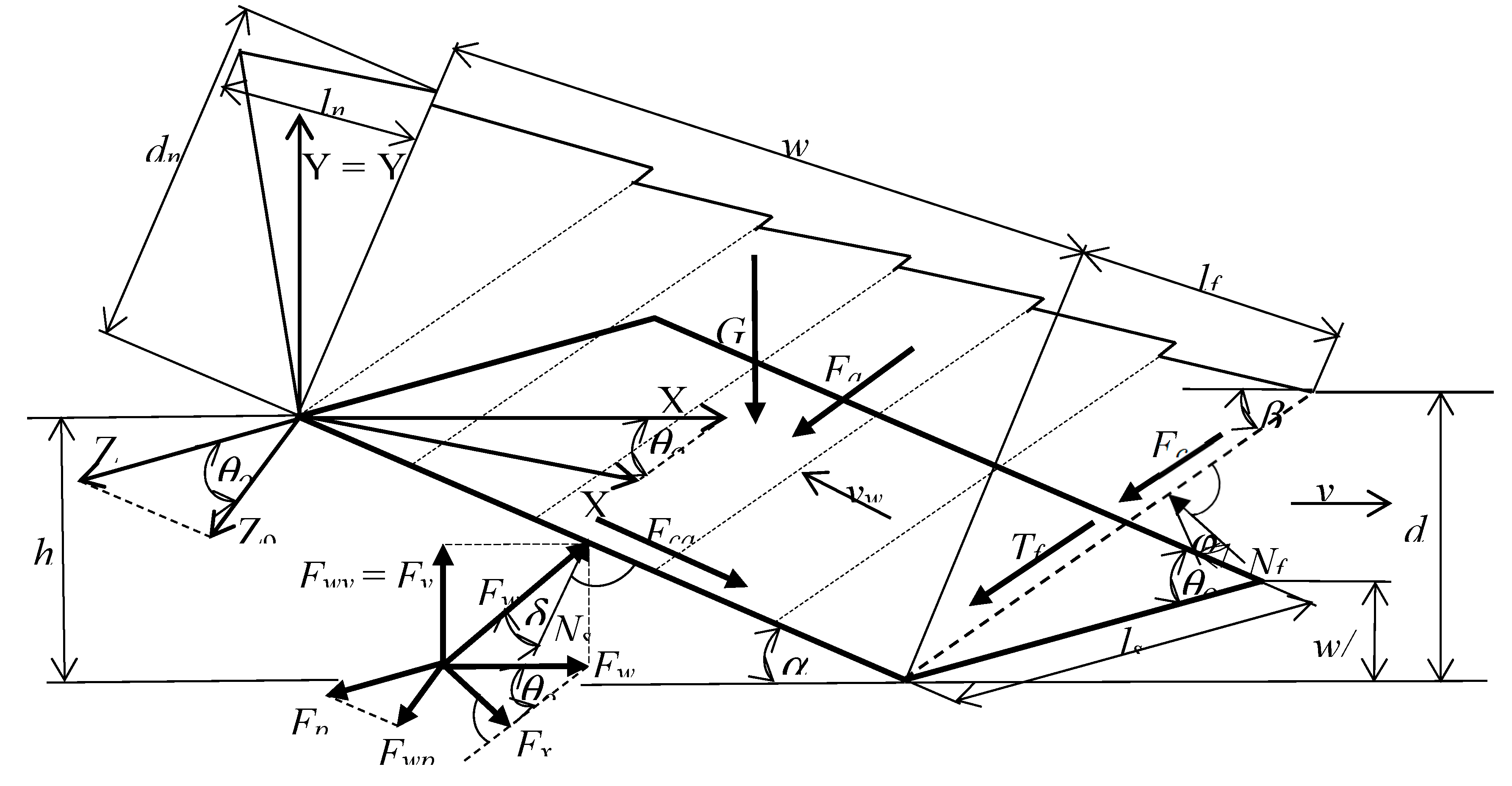
Figure 2.
A comparative diagram of three modified analytical models, Söhne, McKyes, and Perumpral, for duckfoots. Common modifications and advantages (+) and limitations (–) of individual approaches are highlighted
Figure 2.
A comparative diagram of three modified analytical models, Söhne, McKyes, and Perumpral, for duckfoots. Common modifications and advantages (+) and limitations (–) of individual approaches are highlighted
Figure 3.
Comparison of measured Fxe and predictive draught Fxp forces determined from modified Söhne, McKyes, and Perumpral models for the same test conditions.
Figure 3.
Comparison of measured Fxe and predictive draught Fxp forces determined from modified Söhne, McKyes, and Perumpral models for the same test conditions.
Table 1.
The optimal values of φ and external friction angles of δ and shear β for modified Söhne, McKyes, and Perumpral models. For comparison, the angles from the shear test; for soil moisture content MC = 10% were: φ = 37.0°, δ = 24.0°, and β = 31.4°, and for MC = 14% they were: φ = 32.0°, δ = 22.0°, and β = 30.1°.
| Feature |
Söhne |
McKyes |
Perumpral |
|
φ, ° |
d, ° |
b, ° |
φ, ° |
d, ° |
b, ° |
φ, ° |
d, ° |
b, ° |
| All data |
30.00 |
20.00 |
35.00 |
40.00 |
24.38 |
39.64 |
40.00 |
28.77 |
45.00 |
|
MC = 10% |
30.00 |
20.32 |
33.66 |
40.00 |
29.05 |
40.00 |
37.03 |
29.42 |
45.00 |
|
MC = 14% |
30.00 |
20.00 |
35.00 |
40.00 |
20.79 |
40.00 |
40.00 |
27.84 |
45.00 |
Table 2.
Mean values of draught force, experimental Fxe and predictive from the Fxp model, and mean values of mean square errors RMSE, relative δr, and global δg evaluating modified analytical models Söhne, McKyes, Perumpral.
Table 2.
Mean values of draught force, experimental Fxe and predictive from the Fxp model, and mean values of mean square errors RMSE, relative δr, and global δg evaluating modified analytical models Söhne, McKyes, Perumpral.
| Model |
Söhne |
| Feature |
Fxe, N |
Fxp, N |
RMSE, N |
δr, % |
δg, % |
| All data |
238.04 |
246.57 |
64.37 |
-11.58 |
24.95 |
|
MC = 10% |
231.78 |
227.48 |
46.76 |
-3.94 |
18.78 |
|
MC = 14% |
244.30 |
265.66 |
78.12 |
-19.22 |
29.29 |
| Duckfoot = A105 |
195.45 |
177.56 |
57.59 |
-4.54 |
26.81 |
| Duckfoot = B135 |
231.13 |
224.86 |
52.83 |
-4.77 |
21.30 |
| Duckfoot = C200 |
287.56 |
337.29 |
79.53 |
-25.44 |
26.21 |
|
d = 0.03 m |
145.50 |
178.55 |
56.92 |
-33.23 |
36.64 |
|
d = 0.05 m |
234.31 |
246.01 |
53.13 |
-6.01 |
22.06 |
|
d = 0.07 m |
334.33 |
315.15 |
79.80 |
4.49 |
23.28 |
|
v = 0.84 m·s–1
|
200.89 |
243.53 |
65.39 |
-27.94 |
30.45 |
|
v = 1.67 m·s–1
|
236.97 |
246.36 |
55.67 |
-10.46 |
21.85 |
|
v = 2.31 m·s–1
|
276.27 |
249.82 |
71.11 |
3.65 |
23.88 |
| Model |
McKyes |
| All data |
238.04 |
237.38 |
64.39 |
-7.68 |
24.96 |
|
MC = 10% |
231.78 |
210.52 |
50.61 |
3.31 |
20.32 |
|
MC = 14% |
244.30 |
264.24 |
75.70 |
-18.66 |
28.39 |
| Duckfoot = A105 |
195.45 |
174.78 |
58.53 |
-2.49 |
27.25 |
| Duckfoot = B135 |
231.13 |
216.0 |
57.4 |
-0.78 |
23.15 |
| Duckfoot = C200 |
287.56 |
321.35 |
75.62 |
-19.76 |
24.93 |
|
d = 0.03 m |
145.50 |
172.44 |
55.08 |
-29.09 |
35.45 |
|
d = 0.05 m |
234.31 |
236.77 |
52.96 |
-2.20 |
21.99 |
|
d = 0.07 m |
334.33 |
302.92 |
81.24 |
8.26 |
23.70 |
|
v = 0.84 m·s–1
|
200.89 |
234.35 |
59.99 |
-23.49 |
27.93 |
|
v = 1.67 m·s–1
|
236.97 |
237.17 |
54.98 |
-6.51 |
21.58 |
|
v = 2.31 m·s–1
|
276.27 |
240.61 |
76.27 |
6.97 |
25.61 |
| Model |
Perumpral |
| All data |
238.04 |
234.11 |
58.41 |
-3.38 |
22.64 |
|
MC = 10% |
231.78 |
227.29 |
45.13 |
-2.00 |
18.12 |
|
MC = 14% |
244.30 |
241.91 |
68.73 |
-5.70 |
25.77 |
| Duckfoot = A105 |
195.45 |
168.68 |
56.54 |
3.44 |
26.32 |
| Duckfoot = B135 |
231.13 |
213.46 |
49.28 |
2.93 |
19.87 |
| Duckfoot = C200 |
287.56 |
320.20 |
67.89 |
-16.52 |
22.38 |
|
d = 0.03 m |
145.50 |
152.57 |
42.43 |
-13.75 |
27.31 |
|
d = 0.05 m |
234.31 |
232.83 |
47.06 |
-0.28 |
19.54 |
|
d = 0.07 m |
334.33 |
316.94 |
78.86 |
3.89 |
23.00 |
|
v = 0.84 m·s–1
|
200.89 |
230.03 |
53.81 |
-18.00 |
25.06 |
|
v = 1.67 m·s–1
|
236.97 |
233.83 |
49.56 |
-2.38 |
19.46 |
|
v = 2.31 m·s–1
|
276.27 |
238.48 |
69.87 |
10.23 |
23.47 |
|
Disclaimer/Publisher’s Note: The statements, opinions and data contained in all publications are solely those of the individual author(s) and contributor(s) and not of MDPI and/or the editor(s). MDPI and/or the editor(s) disclaim responsibility for any injury to people or property resulting from any ideas, methods, instructions or products referred to in the content. |
© 2025 by the authors. Licensee MDPI, Basel, Switzerland. This article is an open access article distributed under the terms and conditions of the Creative Commons Attribution (CC BY) license (http://creativecommons.org/licenses/by/4.0/).