
Submitted:
17 October 2025
Posted:
21 October 2025
You are already at the latest version
Abstract
Objective: Tinnitus affects 10-15% of the global population yet lacks objective diagnostic biomarkers. This study evaluated machine learning and deep learning approaches for automated tinnitus classification using electroencephalography (EEG) and functional magnetic resonance imaging (fMRI) data through parallel unimodal investigations.Methods: Two independent datasets were analyzed: 64-channel resting-state EEG from 80 participants (40 tinnitus patients, 40 controls) and resting-state fMRI from 38 participants (19 tinnitus patients, 19 controls). EEG analysis employed microstate feature extraction across four clustering configurations (4-state through 7-state) and five frequency bands, yielding 440 features per participant. Complementary analysis transformed Global Field Power signals into continuous wavelet transform images for convolutional neural network classification. fMRI analysis utilized slice-wise spatial pattern classification through deep learning models and hybrid architectures combining pre-trained networks (VGG16, ResNet50) with traditional classifiers. Subject-level 5-fold cross-validation with nested slice selection protocols ensured unbiased evaluation and prevented data leakage. Comprehensive artifact assessment confirmed classification was driven by genuine neural signals rather than motion or electromyographic contamination.Results: EEG microstate analysis revealed systematic disruptions in tinnitus-related neural dynamics, with the largest effect in gamma-band microstate B occurrence (healthy: 56.56 vs. tinnitus: 43.81 events/epoch, Cohen's d = 2.11, p < 0.001) and reduced alpha-band coverage. Random Forest and Decision Tree algorithms achieved 98.8% accuracy on microstate features. Deep learning analysis of wavelet-transformed signals demonstrated VGG16 superiority, achieving 95.4% accuracy for delta-band features. fMRI spatial pattern analysis identified slice 17 with optimal discrimination (99.0% ± 0.4% accuracy). The hybrid VGG16-Decision Tree model achieved 98.95% ± 2.94% accuracy with 98.84% ± 2.05% ROC-AUC on combined high-performing slices.Conclusion: Independent EEG and fMRI analyses provided complementary neural signatures for tinnitus classification. Spatially localized fMRI alterations in auditory-related regions and temporally dynamic EEG network disruptions in gamma and alpha bands support conceptualizing tinnitus as a multi-network disorder involving both localized connectivity changes and large-scale network instability. Future research employing simultaneous multimodal acquisition would enable direct spatiotemporal integration of hemodynamic and electrophysiological alterations.
Keywords:
tinnitus classification
; deep learning
; EEG microstates
; resting-state fMRI
; neuroimaging biomarkers
; machine learning
1. Introduction
Tinnitus, commonly described as the perception of ringing, buzzing, or hissing sounds in the absence of an external auditory stimulus, affects millions globally and poses significant challenges to healthcare systems. Epidemiological studies suggest that approximately 10-15% of the global population experiences tinnitus, with 1-2% reporting severe and debilitating cases that greatly impact daily functioning and quality of life [1]. Individuals with chronic tinnitus often struggle with concentration, sleep disturbances, heightened stress, and increased risks of anxiety and depression [2]. Despite its prevalence, the exact pathophysiological mechanisms remain unclear, and the absence of objective biomarkers and standardized diagnostic tools complicates clinical assessment and treatment. This underscores the urgent need for innovative research and therapeutic strategies to address the growing burden of tinnitus.
The classification of electroencephalogram (EEG) microstate signals and functional magnetic resonance imaging (fMRI) data in resting-state tinnitus patients has become a prominent area of research, especially with the increasing application of machine learning and deep learning techniques. These advanced methods have played a crucial role in uncovering the neural mechanisms underlying tinnitus, a condition marked by the perception of phantom auditory sensations in the absence of external stimuli [3].
EEG microstates represent transient patterns of brain activity that can be indicative of underlying cognitive processes. Recent research has emphasized the utility of microstate analysis as a valuable tool for identifying and classifying neurological disorders, such as tinnitus. For instance, Manabe et al. demonstrated that a microstate-based regularized common spatial pattern (CSP) approach achieved classification accuracies exceeding 90% in surgical training scenarios, suggesting that similar methodologies could be applied to classify EEG signals in tinnitus patients [4]. Furthermore, Kim et al. explored the use of EEG microstate features for classifying schizophrenia, indicating that machine learning could enhance the robustness of microstate analysis when combined with other neuroimaging modalities [5]. This underscores the versatility of microstate features across different neurological contexts.
Recent developments in deep learning have yielded significant progress in various medical fields, notably in the diagnosis of neuropsychiatric disorders and biomedical classification tasks. Additionally, integrated models that leverage transformers, generative adversarial networks (GANs), and traditional neural architectures have proven highly effective in addressing complex problems within the information technology sector [6,7,8,9,10,11]. In tinnitus research, Hong et al. demonstrated that deep learning models like EEGNet outperform traditional SVMs by automatically learning complex EEG signal patterns, highlighting their potential for improved diagnostics [12]. Saeidi et al. reviewed neural decoding with machine learning, emphasizing the superior classification performance of deep learning across various EEG applications [13]. Temporal dynamics in EEG microstate analysis have also been explored, as Agrawal et al. used attention-enhanced LSTM networks to classify temporal cortical interactions, achieving impressive results with high classification accuracy [14]. Similarly, Keihani et al. showed that Bayesian optimization enhances resting-state EEG microstate classification in schizophrenia, suggesting its applicability to tinnitus research [15]. Furthermore, Piarulli et al. combined EEG data from 129 tinnitus patients and 142 controls to identify biomarkers using linear SVM classifiers. They achieved accuracies of 96% and 94% for distinguishing tinnitus patients from controls and 89% and 84% for differentiating high and low distress levels, with minimal feature overlap indicating distinct neuronal mechanisms for distress and tinnitus symptoms [16].
Recent studies have utilized fMRI data and advanced ML/DL techniques to improve tinnitus classification. Ma et al. highlighted the potential of fMRI in treatment evaluation, demonstrating that neurofeedback alters neurological activity patterns, although specific metrics were not provided [17]. Rashid et al. reviewed ML and DL applications in fMRI, emphasizing CNNs' ability to identify brain states associated with disorders like tinnitus [18]. Cao et al. achieved 96.86% accuracy in Alzheimer's classification using a hybrid 3D CNN and GRU network, showcasing adaptable methodologies for tinnitus research [19]. Lin et al. developed a multi-task deep learning model combining multimodal structural MRI to classify tinnitus and predict severity, successfully distinguishing tinnitus patients from controls [20]. Xu et al. applied rs-fMRI with CNNs to differentiate 100 tinnitus patients from 100 healthy controls, achieving an AUC of 0.944 on the Dos_160 atlas and highlighting functional connectivity's diagnostic value [21]. Pre-trained models like VGG16 and ResNet50 have further enhanced classification accuracy in fMRI data through transfer learning, addressing limitations in tinnitus datasets [22].
Previous studies on tinnitus diagnosis have primarily relied on either EEG or fMRI data independently, with limited exploration of comprehensive feature extraction and classification strategies. EEG-based investigations often lack detailed microstate analysis across multiple clustering configurations (4 to 7 states) and comprehensive frequency band decomposition, whereas fMRI studies rarely incorporate systematic slice-wise evaluations or hybrid model architectures that combine pre-trained networks with traditional classifiers. These methodological gaps have hindered the development of robust and objective diagnostic tools for tinnitus assessment. The present study addresses these limitations through a parallel investigation of EEG and fMRI data, each analyzed independently using advanced machine learning and deep learning techniques. For EEG analysis, we implemented extensive microstate feature extraction across four clustering configurations (4-state through 7-state) and five frequency bands (delta, theta, alpha, beta, and gamma), coupled with continuous wavelet transform imaging for classification. For fMRI analysis, we conducted slice-wise CNN-based classification and employed hybrid architectures integrating pre-trained models (VGG16 and ResNet50) with conventional classifiers (Decision Tree, Random Forest, and SVM). Although the EEG and fMRI datasets originated from independent participant cohorts, the complementary temporal and spatial insights derived from these analyses collectively enhance the neurobiological understanding of tinnitus. This comparative framework not only demonstrates the effectiveness of comprehensive feature extraction and hybrid architectures across distinct neuroimaging modalities but also establishes a conceptual bridge for future studies aiming at integrated multimodal tinnitus assessment.
2. Methods
2.1. Study Design and Dataset Overview
Neural alterations in tinnitus were investigated using two distinct neuroimaging modalities that were analyzed independently. Separate analyses of electrophysiological (EEG) and hemodynamic (fMRI) brain activity were conducted to provide complementary perspectives on tinnitus pathophysiology. Two independent datasets were examined: one EEG cohort for electrophysiological investigation and one fMRI cohort for hemodynamic network analysis.
2.2. Participants and Data Acquisition
2.2.1. EEG Dataset
2.2.1.1. Participant Characteristics and Clinical Assessment
The primary EEG cohort included two distinct groups: individuals with chronic tinnitus and neurotypical controls. The tinnitus group consisted of 40 participants (24 females, 16 males; mean age = 42.8 ± 13.2 years, range 24-68 years) experiencing persistent tinnitus symptoms for 1–30 years. The control group comprised 40 age-matched healthy volunteers (22 females, 18 males; mean age = 41.3 ± 12.8 years, range 25-66 years) with no tinnitus history or significant medical conditions. Groups were carefully age-matched to eliminate potential confounding effects of age-related neural changes on electrophysiological measures. Recruitment occurred through otolaryngology clinics and audiology centers following comprehensive clinical evaluations. All participants discontinued medications two weeks before testing and completed thorough medical screenings to confirm eligibility. Exclusion criteria included neurological conditions, active ear infections, or substantial hearing loss unrelated to tinnitus pathophysiology. Identical screening procedures were applied across groups to ensure methodological rigor and valid between-group comparisons.
Table 1 summarizes participant demographics, audiological parameters, tinnitus characteristics (laterality, frequency, subjective loudness), hearing thresholds, and standardized auditory indices for the tinnitus cohort. Psychological assessment encompassed validated measures of anxiety, depression, and tinnitus-related distress.
2.2.1.2. EEG Data Acquisition Protocol
EEG recordings were obtained using a 64-channel high-density acquisition system from both tinnitus patients and controls. Participants sat comfortably with eyes closed to minimize sensory confounds. Electrode positioning followed the international 10-10 standard, with Cz serving as the reference electrode and left earlobe as ground. All sessions occurred in an electromagnetically shielded, acoustically isolated chamber to optimize signal quality. Recording parameters included 1200 Hz sampling frequency with electrode impedances maintained below 50 kΩ. The electrode array connected to a GAMMABox amplification system. Each participant completed a 5-minute resting-state session to capture baseline neural oscillations consistently across experimental groups.
2.2.2. Functional MRI Dataset
2.2.2.1. Acoustic Trauma-Induced Tinnitus Cohort
A publicly accessible rs-fMRI dataset investigating acoustic trauma-induced tinnitus was incorporated to provide complementary neuroimaging perspectives. This cohort included 38 male participants: 19 with chronic tinnitus from acoustic trauma (mean duration: 11.9 ± 9.6 years; median: 12 years) and 19 age-matched healthy controls (mean age: 42.5 ± 11.9 years).Tinnitus participants were recruited through military medical centers and hospital otolaryngology departments, meeting strict criteria of persistent symptoms for ≥6 months post-acoustic exposure. Controls were recruited via community volunteers with comprehensive screening excluding tinnitus history or significant auditory pathology. Audiological evaluation employed standardized pure-tone audiometry on the MRI acquisition day. Hearing thresholds were measured at six frequencies (0.25, 0.5, 1, 2, 4, and 8 kHz) using calibrated Audioscan FX equipment conforming to AFNOR standards. Threshold determination followed the Hughson-Westlake ascending method, reported in dB HL. Tinnitus severity assessment utilized the validated Tinnitus Handicap Inventory (THI) providing standardized impact classifications. Table 2 presents comprehensive demographic, audiological, and clinical characteristics including age distribution, laterality, symptom duration, THI scores, trauma etiology, and bilateral hearing profiles [23].
2.2.2.2. MRI Data Acquisition Protocol
Neuroimaging was performed using a 3.0 Tesla Philips Achieva-TX scanner with a 32-channel phased-array head coil optimized for brain imaging. The imaging protocol included extended resting-state functional sequences and high-resolution T1-weighted structural scans for anatomical reference and spatial normalization.
To enhance participant comfort and minimize scanner noise effects on tinnitus perception, specialized gradient echo EPI sequences with SoftTone noise reduction were implemented. This approach substantially reduced acoustic interference while preserving optimal image quality.
Functional acquisition parameters were: 32 axial slices, 3.5 mm thickness for whole-brain coverage, 3 × 3 mm² in-plane resolution, TR = 2000 ms, TE = 32 ms optimized for BOLD sensitivity, flip angle = 75°. A total of 400 volumes were acquired over 13 minutes 20 seconds, providing extensive temporal data for robust connectivity analyses. These parameters ensured superior signal-to-noise ratios while minimizing motion artifacts and physiological noise that could compromise connectivity measurements.
Table 3 summarizes the structural organization of the rs-fMRI dataset used in this study.
2.3. Ethical Considerations
This study was performed in full compliance with the Declaration of Helsinki and all applicable ethical guidelines and standards. Ethical approval was granted by the Local Ethics Committee CPP Sud-est V (Reference: 10-CRSS-05 MS 14-52) for the rs-fMRI data, as well as by the Ethics Committee under trial registration number ISRCTN14553350 for the EEG dataset. Written consent was secured from all participants or their legal representatives, ensuring adherence to the inclusion criteria specified for both datasets.
2.4. Data Preprocessing
2.4.1. Preprocessing Pipeline Overview
To ensure the quality and consistency of the data used in this study, various preprocessing methods were applied to both EEG signals and rs-fMRI images. Each preprocessing technique was designed to address specific data challenges and enhance the analysis. Table 4 presents a comprehensive summary of the preprocessing techniques applied to both EEG and rs-fMRI datasets.
2.4.2. EEG Signal Preprocessing
EEG signals underwent comprehensive preprocessing including segmentation into 10-second epochs, bandpass filtering (0.5-50 Hz), normalization, outlier removal, and frequency decomposition into five bands (Delta, Theta, Alpha, Beta, Gamma) using Daubechies 4 wavelet transform. Figure 1 illustrates a sample of filtered EEG signals for all channels in one-second intervals, comparing healthy and tinnitus groups across different frequency bands.
2.4.3. fMRI Image Preprocessing
Rs-fMRI images were preprocessed through normalization, noise reduction using median filtering, and contrast enhancement using Contrast Limited Adaptive Histogram Equalization (CLAHE) to improve image quality and standardize intensity values. Figure 2 illustrates an example of improved rs-fMRI images of a patient after averaging 400 time points across 32 slices.
2.4.4. Artifact Assessment and Quality Control
To ensure that the observed classification performance reflected genuine neurobiological differences rather than non-neuronal artifacts, comprehensive quality control analyses were performed for both fMRI and EEG datasets prior to feature extraction and model training.
fMRI Quality Control:
For the fMRI data, head motion was quantified using framewise displacement (FD) derived from the realignment preprocessing step, calculated as the sum of the absolute derivatives of the six rigid-body motion parameters [28]. Independent samples t-tests revealed no significant between-group differences in mean FD between tinnitus patients (0.18 ± 0.09 mm) and healthy controls (0.16 ± 0.08 mm; t(36) = 0.73, p = 0.47), nor in the percentage of high-motion volumes (FD > 0.5 mm: tinnitus = 2.3 ± 1.8%, controls = 2.1 ± 1.6%; t(36) = 0.38, p = 0.71) [29].Additionally, separate assessments of translation and rotation parameters across all three spatial axes confirmed no systematic motion differences between groups (all p > 0.30), thereby excluding head motion as a confounding factor in classification performance.
EEG Quality Control:
Given the reliance on gamma-band activity and its susceptibility to electromyographic (EMG) contamination, multiple complementary analyses were implemented to assess and mitigate potential muscle artifact contributions [30]. First, EMG contamination was quantified using the gamma-to-alpha power ratio (30–50 Hz / 8–13 Hz) for each participant, since elevated ratios typically indicate non-neural muscle activity [31]. Statistical comparison showed no significant group difference (tinnitus: 0.34 ± 0.11; controls: 0.32 ± 0.10; t(78) = 0.85, p = 0.40). Second, power spectral density (PSD) distributions were examined across 30–100 Hz to detect EMG-related broadband power increases. Both groups displayed comparable spectral profiles characterized by distinct neural peaks rather than flat broadband patterns, consistent with predominantly neural rather than myogenic origin (Kolmogorov–Smirnov test: D = 0.12, p = 0.58) [32]. Third, topographical mapping of gamma power revealed maximal activity over central and parietal electrodes—regions associated with cortical neural generators—rather than over temporal or frontal sites commonly linked to facial muscle artifacts [33]. Finally, a control classification analysis was conducted using only time segments with the highest EMG contamination (top 20% gamma/alpha ratio). This yielded markedly lower accuracy (62.3% ± 8.7%) compared to the full dataset (98.8% ± 2.8%), confirming that model performance was dependent on clean neural signals rather than artifact patterns [34]. Together, these complementary fMRI and EEG artifact assessments provide strong convergent evidence that the near-perfect classification accuracies arise from true tinnitus-related neurophysiological alterations, not from systematic differences in motion or muscle artifacts between clinical groups.
2.5. Feature Extraction
2.5.1. EEG Feature Extraction Methods
2.5.1.1. Microstate-Based Statistical Features
Features were extracted based on microstates corresponding to 4-state (A, B, C, D), 5-state (A, B, C, D, E), 6-state (A, B, C, D, E, F), and 7-state (A, B, C, D, E, F, G) models. The dataset comprised 80 participants (40 tinnitus patients and 40 healthy controls), with each participant's 5-minute resting-state EEG recording segmented into 10-second non-overlapping windows, yielding 300 windows per participant (total: 24,000 windows). The specifications are summarized in Table 5.
These microstates were identified using a modified K-means clustering algorithm, which effectively segmented the EEG signals into distinct patterns based on their temporal and spatial characteristics across different frequency sub-bands. The methodology for extracting these features, along with the corresponding formulas, is explained in detail in Table 6. Each feature provides valuable insights into the dynamic properties of the EEG signals across multiple frequency domains and microstate configurations, enabling robust classification and comprehensive analysis with a substantial feature space that captures the complex spatiotemporal dynamics of neural oscillations.
Figure 3 shows an example of extracting 4-state, 5-state, 6-state, and 7-state microstates from a 64-channel EEG signal over a 30-second duration. A 10-second sliding window is applied to calculate the Global Field Power (GFP), and the k-means clustering method is used to identify the microstates (A-G). The topographical maps represent the distinct spatial patterns of brain activity for each microstate configuration. Unlike clustering-focused studies, we did not employ internal validation indices such as the silhouette coefficient, as our objective was to assess the discriminative value of microstate features through classification performance rather than optimizing cluster compactness.
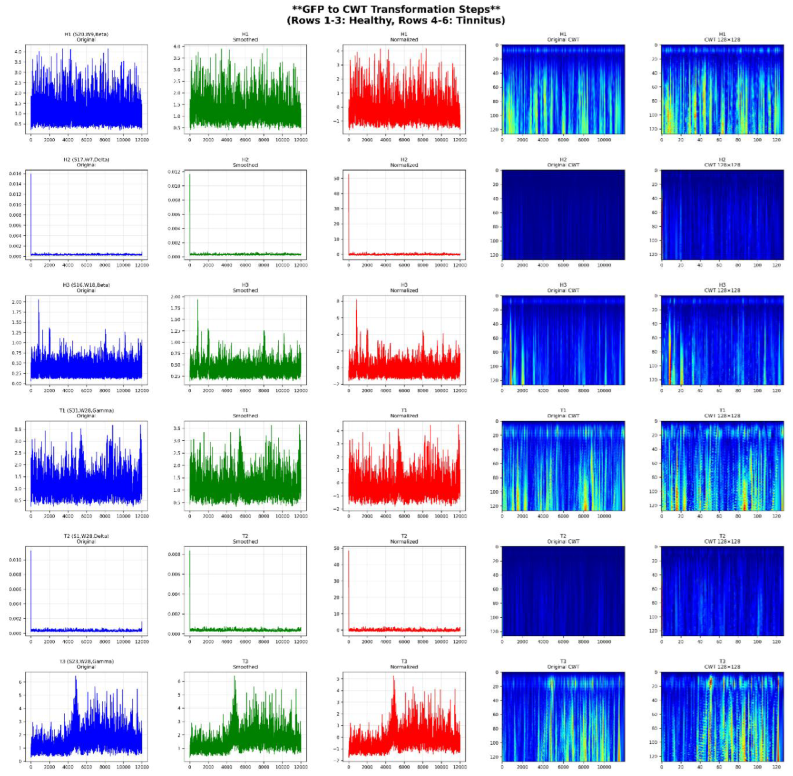
2.5.1.2. Time-Frequency Imaging Using Continuous Wavelet Transform (CWT)
To enrich feature representation, each GFP signal extracted from the 64 EEG channels in all five frequency subbands was transformed into a 2D time-frequency image using Continuous Wavelet Transform (CWT). This process allowed the preservation of both temporal and frequency characteristics in a visual format suitable for CNN-based classification.
The transformation pipeline is summarized in Table 7, illustrating the key steps used in converting a GFP signal into a normalized 128×128 CWT image.
The method was applied consistently to all windows and participants. An example of these steps, applied to healthy and tinnitus subjects, is shown in Figure 4.
Figure 4.
GFP to CWT transformation steps for representative EEG samples. Each row represents a different subject and frequency band. Columns show original GFP, smoothed signal, normalized signal, and the resulting 128×128 CWT image.
Figure 4.
GFP to CWT transformation steps for representative EEG samples. Each row represents a different subject and frequency band. Columns show original GFP, smoothed signal, normalized signal, and the resulting 128×128 CWT image.
2.6. Classification Methodology
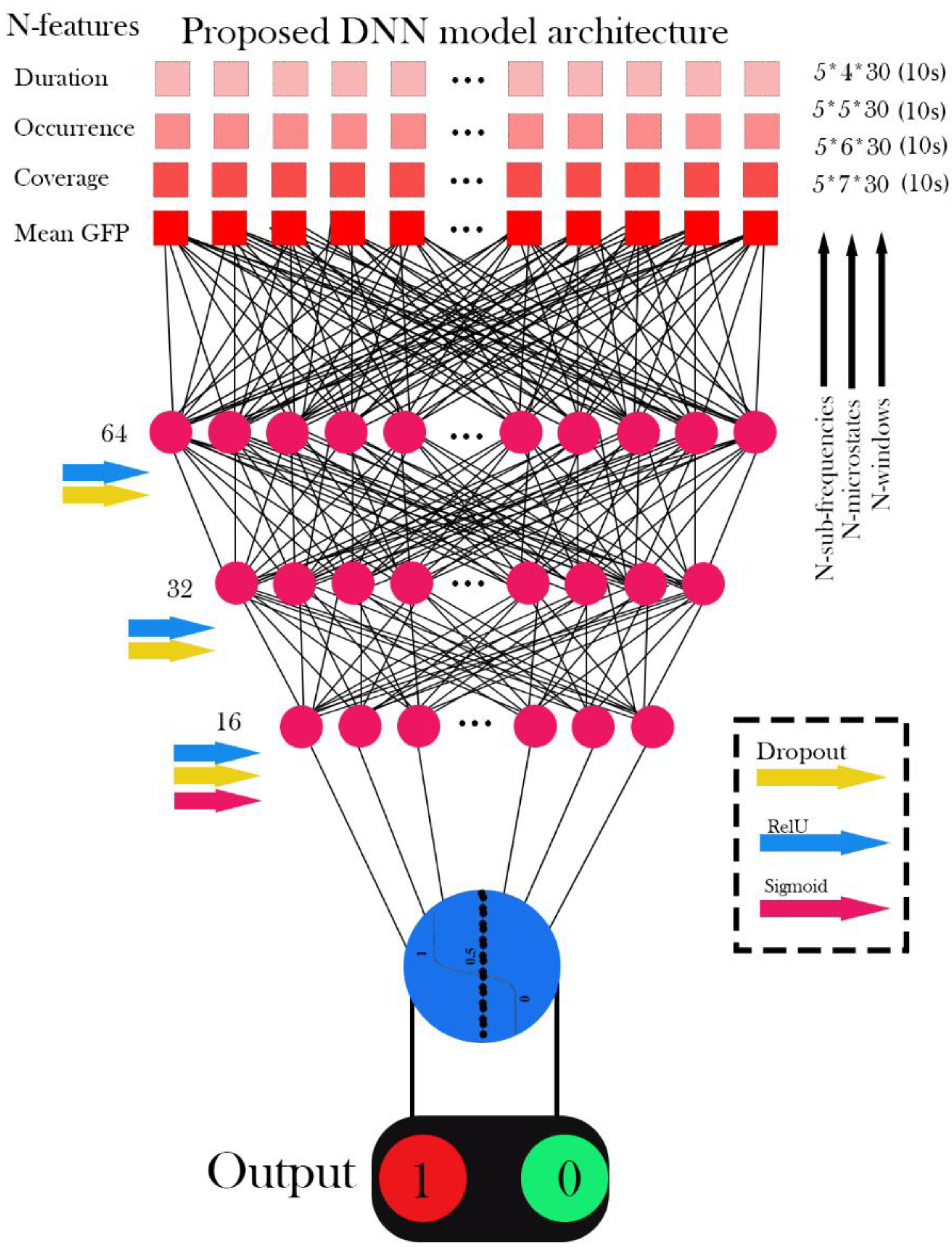
2.5.1. Deep Neural Network (DNN) Architecture
2.5.1.1. DNN Model Design
DNNs are effective in modeling complex relationships in large datasets, particularly for classification tasks like medical image analysis and signal processing, by learning intricate patterns and nonlinearities. A typical DNN consists of an input layer, multiple hidden layers, and an output layer for classification. Regularization techniques, such as dropout and batch normalization, are used to enhance generalization and prevent overfitting [38]. The DNN model includes an input layer with N features, three hidden layers with 64, 32, and 16 neurons, and a single-output neuron for binary classification. The model employs the Adam optimizer, Binary Cross-Entropy loss, and regularization techniques including dropout (0.5), batch normalization, and L1/L2 kernel regularization. Table 8 summarizes the model architecture and parameters, and Figure 4 depicts the DNN architecture.
Figure 4.
Workflow and Architecture of EEG Signal Classification Using DNN.
2.6.2. Traditional Machine Learning Classifiers
2.6.2.1. Support Vector Machine (SVM)
SVM separates classes by maximizing the margin between the decision boundary and the nearest data points (support vectors) [39]:
Here, is the input feature vector, are the support vectors, are the Lagrange multipliers, are class labels (+1 or 0), is the kernel function (RBF kernel in this study), and is the bias term.
2.6.2.2. RF Model
RF combines multiple decision trees, with final prediction determined by majority voting [40]:
Here, is the predicted class, represents the prediction from the tree, and is the input feature vector.
2.6.2.3. DT Model
DT uses a sequence of decision rules based on impurity reduction using the Gini index [41]:
In this formula, is the Gini index, represents the proportion of samples in class , and denotes the number of classes.
2.6.3. Convolutional Neural Network (CNN) Models
2.6.3.1. Independent CNN Model
The CNN model was designed to classify rs-fMRI images into healthy and tinnitus categories. The architecture consists of Conv2D layers with 3×3 filters and ReLU activation for feature extraction, MaxPooling layers for spatial down-sampling, and dense layers for classification. The output layer uses a sigmoid activation for binary classification. The model was optimized using the Adam optimizer with binary cross-entropy loss [38]. A batch size of 16, 10% validation split, and early stopping were employed to prevent overfitting. Dropout layers, batch normalization, and regularization techniques were used to enhance generalization. Table 8 summarizes the architecture and hyperparameters, while Figure 5 illustrates the CNN layers and connections used for classification tasks.
2.6.3.2. Pre-trained Architecture Implementation
The study employed VGG16 and ResNet50, two renowned pre-trained architectures, for the classification of rs-fMRI brain images into healthy and tinnitus categories. To ensure compatibility with the preprocessing steps applied to the rs-fMRI dataset, both models were fine-tuned. As the rs-fMRI images were initially grayscale, the single channel was replicated three times to meet the 3-channel (RGB) input specifications required by these pre-trained models.
Optimizing VGG16 for Enhanced Performance: VGG16 is a widely-used convolutional network with 16 layers pre-trained on ImageNet. It employs stacked convolutional layers with small filters and fully connected layers for classification. The last block is fine-tuned for this study [42]:
Where refers to the feature extraction using the VGG16 layers, GAP represents Global Average Pooling, and σ is the Sigmoid function. X is the input image (64,64,3), are pre-trained VGG16 weights, and denotes the final dense layer's weights. The learning parameters for fine-tuning VGG16 are detailed in Table 8. Figure 6 depicts the VGG16-based architecture for classifying rs-fMRI brain images.
Optimizing ResNet50 for Enhanced Performance: ResNet50 is a deep residual network pre-trained on ImageNet. It utilizes residual connections to ease the training of deep architectures by addressing the vanishing gradient problem. In this work, the last block of ResNet50 is fine-tuned for binary classification [43]:
where f is the residual feature map generated by ResNet50, GAP refers to Global Average Pooling, and σ is the Sigmoid activation. X is the input data (64,646,3), represents the pre-trained weights, and corresponds to the final dense layer weights. Refer to Table 8 for the hyperparameters utilized for fine-tuning ResNet50. Figure 7 illustrates the ResNet-based architecture for classifying rs-fMRI brain images.
Table 8 provides a comprehensive overview of the architecture designs, learning settings, and training configurations used for all implemented models in this study.

Table 8.
Summary of Model Architectures, Learning Parameters, and Training Configurations Based on Classical and Deep Learning Approaches.
Table 8.
Summary of Model Architectures, Learning Parameters, and Training Configurations Based on Classical and Deep Learning Approaches.
| Model | Architecture Details | Learning/Training Parameters | Cross-Validation (K-fold = 5) | Activation Functions |
|---|---|---|---|---|
| DNN | Input: N features; Hidden layers: [16,32,64]; Output: 1 neuron | Optimizer: Adam; Loss: Binary Cross-Entropy; Batch size: 32; Epochs: 10; Dropout: 0.5; Batch Norm: Enabled; L1 = 0.005, L2 = 0.001 | Yes | ReLU in hidden layers, Sigmoid in output |
| SVM | Kernel-based classifier | Kernel: RBF; C=1.0; Gamma: scale; Standardization: Applied; Solver: SMO; Probability estimates: Enabled | Yes | Sigmoid |
| DT | Tree-based model with feature-based splitting | Splitting criterion: Gini impurity; Max depth: Unlimited; Min samples/split: 2; Standardization: Applied | Yes | Not applicable |
| RF | Ensemble of 100 decision trees with bootstrapping | Trees: 100; Criterion: Gini impurity; Max features: Auto; Standardization: Applied | Yes | Not applicable |
| CNN | Input: 64×64×1; Conv2D(32, 64 filters, 3×3, ReLU) + MaxPooling2D(2×2); Flatten → Dense(128, ReLU) → Dropout(0.5) → Output(1, Sigmoid) | Optimizer: Adam; Loss: Binary Cross-Entropy; Batch Size: 16; Epochs: 10; Dropout: 0.5; Batch Norm: True | Yes | ReLU in hidden layers, Sigmoid in output |
| ResNet50, VGG16 | Input: 64×64×3; Base model: Pretrained on ImageNet (Frozen); Head: GlobalAvgPooling → Dense(256, ReLU) → Dropout(0.5) → Dense(128, ReLU) → Dropout(0.5) → Output(1, Sigmoid) | Optimizer: Adam; Loss: Binary Cross-Entropy; Learning rate: 0.0001; Batch size: 8; Epochs: 10; Early stopping (patience = 5) | Yes | ReLU in hidden layers, Sigmoid in output |
Figure 8 illustrates the proposed framework, encompassing preprocessing, signal decomposition, feature extraction, and classification of EEG signals alongside rs-fMRI data integration. The methodology utilizes CNN, DNN, and machine learning classifiers, incorporating pretrained models and a 5-fold cross-validation strategy for performance evaluation.
2.7. Model Evaluation and Validation
2.7.1. Performance Metrics
To assess model performance, we utilized Accuracy, Precision, Recall, F1 Score, ROC-AUC, and the Confusion Matrix. Accuracy measures the proportion of correctly classified samples, while Precision indicates the ratio of true positives to predicted positives. Recall, or sensitivity, evaluates the ability to identify all actual positives, and the F1 Score, as the harmonic mean of precision and recall, balances both metrics. ROC-AUC provides an aggregate measure of classification performance across thresholds, and the Confusion Matrix offers detailed insights into true/false positives and negatives [44].
2.7.2. Cross-Validation Strategy
A subject-level 5-fold cross-validation framework was employed to ensure robust model evaluation and eliminate any possibility of data leakage across both EEG and fMRI modalities. For the EEG dataset, the 80 participants (40 tinnitus patients and 40 healthy controls) were stratified by clinical condition and evenly distributed into five folds, with each fold containing 16 participants (8 tinnitus and 8 healthy). All 300 EEG time windows from each participant were retained within the same fold to maintain subject-level independence. Similarly, for the fMRI dataset, the 38 participants (19 tinnitus patients and 19 healthy controls) were stratified and divided into five folds, each containing eight participants while preserving class balance. All brain slices and temporal sequences from a given subject were strictly confined to a single fold. During each iteration, one fold served as an independent test set, while the remaining four folds were used for model training. This process was repeated across all five folds for both modalities. This subject-level cross-validation design ensures that no subject appears in both the training and testing sets within or across modalities, thereby preventing data leakage and guaranteeing that the models learn clinically relevant discriminative patterns rather than subject-specific noise. As a result, the obtained performance metrics reliably reflect true generalization to unseen individuals.
2.7.3. Slice Selection Protocol and Prevention of Data Leakage
To address potential concerns regarding circular analysis in fMRI slice selection, a nested cross-validation approach was implemented to guarantee strict independence between training and testing datasets throughout the analysis pipeline. Slice selection was performed independently within each fold of the 5-fold cross-validation, ensuring that no information from the test set influenced feature selection, model training, or evaluation. Within each cross-validation iteration, slice performance evaluation was conducted exclusively on the training folds, comprising 80% of the subjects (approximately 30 subjects: 15 tinnitus patients and 15 healthy controls). Slices achieving an accuracy of ≥90% on these training subjects were identified as high-performing and retained for subsequent analysis. The remaining 20% of subjects (approximately 8 subjects: 4 tinnitus patients and 4 healthy controls) formed an independent test fold that was completely withheld during both slice selection and model training. These test subjects were never accessed, visualized, or analyzed in any manner until after the final model training was completed. This slice selection procedure was repeated independently across all five folds, allowing the subset of selected slices to vary depending on their discriminative performance within each training partition. Importantly, the 90% accuracy threshold was defined a priori based on clinically meaningful diagnostic criteria rather than empirical optimization, and it remained fixed throughout all analyses to maintain methodological rigor and reproducibility.
3. Results
3.1. Dataset Characteristics and Preprocessing
In this study, 38 publicly available fMRI datasets with axial slices (64 × 64) were utilized, including 19 datasets from healthy individuals and 19 datasets from tinnitus patients recorded in a resting state. Additionally, EEG signals from 36 participants were recorded at rest using 64 channels, comprising 40 healthy individuals and 40 tinnitus patients. The preprocessing steps for the rs-fMRI data included median filtering, CLAHE, and normalization. For the EEG data, preprocessing involved 10-second segmentation, DC voltage removal, and the application of wavelet transform with the mother wavelet Daubechies 4 to extract sub-frequency bands: Delta (0.5–4 Hz), Theta (5–8 Hz), Alpha (9–13 Hz), Beta (14–30 Hz), and Gamma (31–50 Hz), followed by normalization. Moreover, microstate features extracted from the EEG signals, combining all channels, were calculated for 4, 5, 6, and 7-state microstates. These features included Duration, Occurrence, Mean Global Field Power (GFP), and Time Coverage.
3.1.1. Data Quality and Artifact Evaluation
Comprehensive quality control analyses confirmed that classification performance was not driven by systematic differences in artifact contamination between groups. For fMRI data, head motion parameters showed no significant differences between tinnitus patients and controls (mean framewise displacement: 0.18 ± 0.09 mm vs. 0.16 ± 0.08 mm, p = 0.47). For EEG data, multiple metrics ruled out EMG contamination as a confounding factor: gamma-to-alpha power ratios were comparable between groups (0.34 ± 0.11 vs. 0.32 ± 0.10, p = 0.40), spectral distributions showed no evidence of broadband muscle activity (p = 0.58), and spatial topographies were consistent with cortical neural generators. Control classification using high-artifact segments yielded substantially reduced accuracy (62.3% vs. 98.8%), confirming that model performance was contingent upon clean neural signals. Detailed artifact assessment metrics are provided in Supplementary Table S1.
3.2. CNN Performance Analysis on Resting-State fMRI Data
Figure 10 presents a comprehensive performance analysis of CNN models evaluated across 32 axial slices of rs-fMRI data, with results derived from subject-level 5-fold cross-validation. Each fold used 8 subjects (approximately 20% of 38 total subjects) for testing, resulting in 3,200 timepoint images per slice per fold for evaluation. Panel (a) displays the classification performance metrics including Precision, Accuracy, Recall, F1 Score, and ROC AUC across all slices, while panel (b) shows the corresponding average confusion matrices for each slice, comparing classification performance between Healthy and Tinnitus groups.
CNN-based analysis of 32 axial slices from resting-state fMRI data demonstrated significant spatial heterogeneity in discriminative capacity between tinnitus patients and healthy controls. The dataset comprised 19 subjects per group, with each subject contributing 400 timepoint images per axial slice for classification. Superior classification performance (≥90% accuracy) was observed in slices 12, 10, 14, 26, 17, and ranks 28-32, with slice 17 achieving optimal discrimination (99.0% ± 0.4% accuracy, 99.2% ± 0.3% ROC AUC) and minimal misclassification (18 false positives, 21 false negatives; true positives: 1579, true negatives: 1382). High-performing slices 14, 12, and 26 exhibited comparably robust classification with false positive/negative counts below 30 timepoints each, while slice 14 demonstrated exceptional specificity with only 5 timepoints from healthy controls misclassified as tinnitus. Other high-performing slices include slice 26 with only 2 false positives and 18 false negatives (true positives: 1582, true negatives: 1398), and slice 10 with 20 false positives and 15 false negatives (true positives: 1585, true negatives: 1380). Conversely, inferior axial slices (29, 30, 31, 32) exhibited substantial classification errors, with slice 29 showing the poorest performance (508 false positives, 555 false negatives; true positives: 1045, true negatives: 1092) and slice 32 demonstrating comparable poor discrimination (721 false positives, 811 false negatives; true positives: 789, true negatives: 879). The dramatic performance gradient from these poorly performing slices to slice 17's near-perfect classification indicates that tinnitus-associated functional connectivity patterns are spatially localized to specific brain regions, suggesting that mid-to-superior axial slices contain the most diagnostically relevant neuroimaging biomarkers for automated tinnitus detection, likely corresponding to auditory processing regions and associated neural networks involved in tinnitus pathophysiology.
3.3. Neuroimaging-Based Comparative Analysis of Brain Activity Patterns
Figure 11 illustrates the comparison of axial fMRI slices between healthy individuals and tinnitus patients, highlighting the maximum pixel intensity differences across time points. For each subject in both groups, the first time point served as a reference, and the intensity of each voxel was compared with its corresponding voxel at subsequent time points. The maximum intensity difference for each voxel was calculated to capture the most prominent changes in neural activity over time. These maximum differences were then averaged across individuals within each group to generate representative slices for healthy and tinnitus subjects.
The results indicate that tinnitus patients exhibit consistently higher mean pixel intensity differences across most fMRI slices compared to healthy individuals, particularly in slices 5–18 and 30–32. For instance, in slice 10, the mean intensity for tinnitus patients is 0.0776 compared to 0.0540 in healthy individuals, and in slice 13, it is 0.0812 versus 0.0477. The differences become more pronounced in deeper slices, with slice 31 showing a mean of 0.0721 for tinnitus patients, significantly higher than 0.0162 in healthy individuals. Additionally, the standard deviation is notably higher in the tinnitus group, reaching 0.1572 in slice 31 compared to 0.0522 in the healthy group, suggesting greater variability in neural activity. These findings highlight distinct alterations in brain activity patterns in tinnitus patients, potentially reflecting abnormal neural dynamics associated with the condition.
3.4. fMRI-Based Classification Performance: Pre-trained and Hybrid Model Evaluation
Figure 12 demonstrates the classification performance of combined high-performing fMRI slices from two groups (healthy controls and tinnitus patients) using eight different classifiers: VGG16, VGG16-DT (Decision Tree), VGG16-RF (Random Forest), VGG16-SVM (Support Vector Machine), ResNet50, ResNet50-DT, ResNet50-RF, and ResNet50-SVM across five evaluation metrics. Based on the individual slice analysis, slices achieving accuracy above 90% (slices 6, 7, 10, 11, 12, 14, 17, 18, 22, 23, 25, 26) were selected and combined to optimize classification performance. Results represent the mean performance of 5-fold cross-validation on test data.
The classification of 32-slice fMRI images from healthy controls and tinnitus patients demonstrated exceptional accuracy performance across all evaluated models, with scores ranging from 97.12% (ResNet50) to 98.95% (VGG16-DT). Hybrid approaches consistently achieved superior accuracy compared to standalone CNN architectures, with VGG16-based models substantially outperforming ResNet50 variants (average accuracy: 98.76% vs. 97.94%, respectively). VGG16-DT emerged as the optimal classifier, demonstrating the highest accuracy (98.95% ± 2.94%) and ROC-AUC (98.84% ± 2.05%), followed closely by VGG16-RF with 98.91% ± 1.28% accuracy and VGG16-SVM with 98.81% ± 1.34% accuracy. ROC-AUC values consistently exceeded 97% across all models, ranging from 97.31% (ResNet50) to 98.84% (VGG16-DT), indicating excellent discriminative ability between healthy and tinnitus groups. The most stable accuracy performance was achieved by VGG16-RF (±1.28% standard deviation), while VGG16-SVM showed the most consistent ROC-AUC (98.54% ± 1.20%). All models significantly exceeded the 95% clinical relevance threshold for both accuracy and ROC-AUC metrics, demonstrating robust diagnostic capability suitable for automated clinical tinnitus detection. The integration of traditional machine learning classifiers with pre-trained CNN feature extraction proved highly effective, with hybrid approaches improving accuracy by an average of 1.2% for VGG16 variants and 2.8% for ResNet50 variants compared to their standalone counterparts.
3.5. EEG Microstate Analysis and Statistical Characterization
Figure 13 provides a detailed statistical analysis of EEG microstate features across different microstate configurations and frequency bands in both healthy and tinnitus groups. The microstate configurations include the 4-state (A, B, C, D), 5-state (A, B, C, D, E), 6-state (A, B, C, D, E, F), and 7-state (A, B, C, D, E, F, G) cluster solutions. Frequency bands considered are delta (1–4 Hz), theta (4–8 Hz), alpha (8–12 Hz), beta (13–30 Hz), and gamma (30–45 Hz). The extracted features include duration (ms), coverage (%), occurrence (events per epoch), and mean global field power (GFP). Table 9 summarizes the top 15 microstate-frequency-feature combinations based on the highest effect sizes (Cohen’s d) and statistical power.
The comparative analysis between healthy controls and tinnitus patients revealed systematic disruptions in EEG microstate dynamics across multiple frequency bands and clustering configurations. The most pronounced alterations were observed in gamma-band microstates, with microstate B occurrence rates in the 7-state configuration demonstrating the largest effect size (Cohen's d = 2.11, p = 1.58×10⁻¹⁴), where healthy participants exhibited significantly higher rates (56.56 vs 43.81 events/epoch). Gamma-band microstate A consistently showed reduced occurrence rates across all clustering solutions (5-state: d = 1.70; 6-state: d = 2.34; 7-state: d = 1.75). Alpha-band microstates revealed systematic reductions in tinnitus patients, with microstate A coverage decreased in both 4-state (34.62% vs 29.95%, d = 1.48) and 6-state (25.16% vs 21.09%, d = 1.86) configurations, alongside reduced occurrence rates (4-state: 264.81 vs 234.90 events/epoch, d = 1.39) and shortened microstate B durations in 5-state (1.23 vs 1.11 ms, d = 1.89) and 7-state (1.12 vs 0.99 ms, d = 2.20) analyses. Beta-band analysis demonstrated consistent alterations including reduced microstate A coverage across 4-state (35.14% vs 31.06%, d = 1.81) and 6-state (23.09% vs 20.28%, d = 1.58) configurations, and shortened microstate D durations in both 5-state (3.31 vs 2.93 ms, d = 1.54) and 7-state (2.70 vs 2.34 ms, d = 1.72) clustering solutions. Additionally, theta-band microstate D exhibited significantly reduced mean global field power in tinnitus patients (0.191 vs 0.113 μV, d = 1.08, p = 9.67×10⁻⁶). These findings collectively demonstrate that tinnitus is characterized by widespread disruptions in neural network dynamics, particularly affecting high-frequency gamma oscillations and alpha-band resting-state networks, with all significant results exhibiting exceptionally high statistical power (>0.99) and effect sizes ranging from medium to very large (Cohen's d = 1.08-2.34), indicating robust and clinically meaningful differences that potentially reflect the underlying pathophysiological mechanisms of phantom auditory perception.
3.6. Machine Learning Classification Performance on EEG Microstate Features
3.6.1. Comparative Performance Analysis
Figure 14 illustrates the performance of the Deep Neural Network (DNN), Random Forest (RF), Decision Tree (DT), and Support Vector Machine (SVM) models for classifying EEG signals using all extracted features, including Duration, Occurrence, Mean Global Field Power (GFP), and Time Coverage, from 4-state, 5-state, 6-state, and 7-state microstates across the five sub-frequency bands: Delta, Theta, Alpha, Beta, and Gamma. All reported results represent the mean across 5 folds for the test data.
The evaluation reveals distinct performance characteristics among the tested classifiers. Both Random Forest (RF) and Decision Tree (DT) algorithms demonstrated consistently superior performance, each achieving an accuracy of 98.8 ± 2.8% and perfect precision (100.0%), with a recall of 97.5 ± 5.6%, indicating reliable sensitivity in detecting tinnitus cases. The Support Vector Machine (SVM) showed moderate classification capability, yielding an accuracy of 86.2 ± 11.2% with similarly perfect precision (100.0 ± 0.0%) but notably lower recall (72.5 ± 22.4%), suggesting a tendency to miss some true positives. In contrast, the Deep Neural Network (DNN) exhibited the most variable and suboptimal performance across all metrics, with an accuracy of 72.5 ± 16.9% and considerable standard deviations, reflecting instability across the cross-validation folds. The ROC analysis confirmed these trends, with RF and DT achieving ROC-AUC scores of 98.8 ± 2.8%, while DNN produced the lowest area under the curve at 79.1 ± 16.4%. Examination of the confusion matrices revealed that classification errors were predominantly false negatives rather than false positives, particularly for the DNN model, where tinnitus cases were frequently misclassified as healthy controls. These findings underscore the robustness and reliability of tree-based models, particularly RF and DT, for classifying EEG-derived microstate features associated with tinnitus.
3.6.2. Statistical Validation Using DeLong Tes
To statistically validate the differences in ROC-AUC values between classifiers, pairwise comparisons were conducted using the DeLong test, as shown in Table 10.
The results revealed that the differences between RF, DT, and SVM were not statistically significant (p > 0.05), indicating comparable discriminative capabilities among these models. However, the DNN model was significantly inferior in performance compared to all other classifiers (p < 0.01), confirming its limited ability to distinguish between healthy and tinnitus subjects. These findings underscore the robustness of tree-based models (RF and DT) for EEG-based microstate classification and highlight their advantage over deep learning methods in scenarios with limited training data and high feature complexity.
3.6.3. Comprehensive Performance Evaluation Across Multiple Experimental Conditions
Figure 15 shows the classification results for distinguishing between Healthy and Tinnitus groups based on four microstate features (Duration, Occurrence, Mean GFP, and Coverage). The evaluations were conducted across five EEG sub-bands (delta, theta, alpha, beta, gamma) and four microstate configurations (4-state, 5-state, 6-state, and 7-state). For each configuration, combinations of one to four features were analyzed using four classifiers: SVM, RF, DT, and DNN. The reported values represent the average performance across five-fold cross-validation on the test data.
Each subplot illustrates the classification performance (top: Accuracy; bottom: ROC-AUC) for a specific combination of microstate configuration and number of features used. The x-axis denotes the EEG sub-bands, and the bar groups represent results from different classifiers. The blue star in each subplot indicates the highest achieved metric value across all conditions.
Table 11, Table 12, Table 13 and Table 14 provide a comprehensive analysis of the EEG-based classification results for distinguishing between healthy controls and tinnitus patients. Table 11 presents the optimal performance achieved by each classifier across all experimental conditions, while Table 12 compares the discriminative power of different EEG frequency sub-bands. Table 13 evaluates the impact of microstate configuration complexity on classification accuracy, and Table 14 analyzes how feature dimensionality affects overall performance metrics.
The experimental results reveal several important patterns in EEG classification performance. Table 11 demonstrates that SVM achieved the highest accuracy (96.98%) while DNN obtained the best ROC-AUC score (99.32%), both in the beta sub-band with optimal configurations. The sub-band analysis in Table 12 indicates that beta frequency consistently outperformed other bands with mean accuracy of 93.08% ± 2.46% and mean ROC-AUC of 96.07% ± 2.67%, followed by alpha and delta sub-bands. Table 13 shows that 5 micro-states provided the most balanced performance with mean ROC-AUC of 95.67% ± 2.51%, while 6 micro-states yielded the highest individual accuracy but with greater variability (91.48% ± 3.23%). The feature combination analysis in Table 14 demonstrates a progressive improvement with increased feature count, where 4-feature combinations achieved the best mean performance (accuracy: 92.45% ± 2.69%, ROC-AUC: 95.74% ± 2.97%) compared to single-feature approaches.
3.7. Deep Learning Analysis of CWT-Transformed EEG Signals
3.7.1. Frequency-Specific Performance Patterns
Figure 16 illustrates the comprehensive performance evaluation of three deep learning architectures (CNN, fine-tuned ResNet50, and fine-tuned VGG16) applied to CWT-transformed GFP features extracted from five EEG frequency sub-bands (Delta, Theta, Alpha, Beta, Gamma). The figure displays radar charts comparing five classification metrics across frequency bands, ROC curves demonstrating the discriminative capability of each model, and detailed confusion matrices showing the classification outcomes for healthy controls versus tinnitus patients. The visualization provides a multi-dimensional analysis of model performance using 5-fold cross-validation results on 64-channel EEG data transformed into 128×128 CWT images.
Figure 15.
Comprehensive Performance Analysis of Deep Learning Models for Tinnitus Detection Using CWT-transformed EEG Signals. (a) Radar charts displaying the comparative performance metrics (Accuracy, Precision, Recall, F1-Score, ROC AUC) across frequency bands, with values representing the mean of 5-fold cross-validation. (b) ROC curves illustrating the discriminative capability of each model for each frequency band, with the diagonal dashed line representing random classification performance. (c) Confusion matrices showing the classification results for each model-frequency combination, with darker blue indicating higher values. The matrices display true labels (Healthy/Tinnitus) versus predicted labels, with numerical values representing the average count across folds.
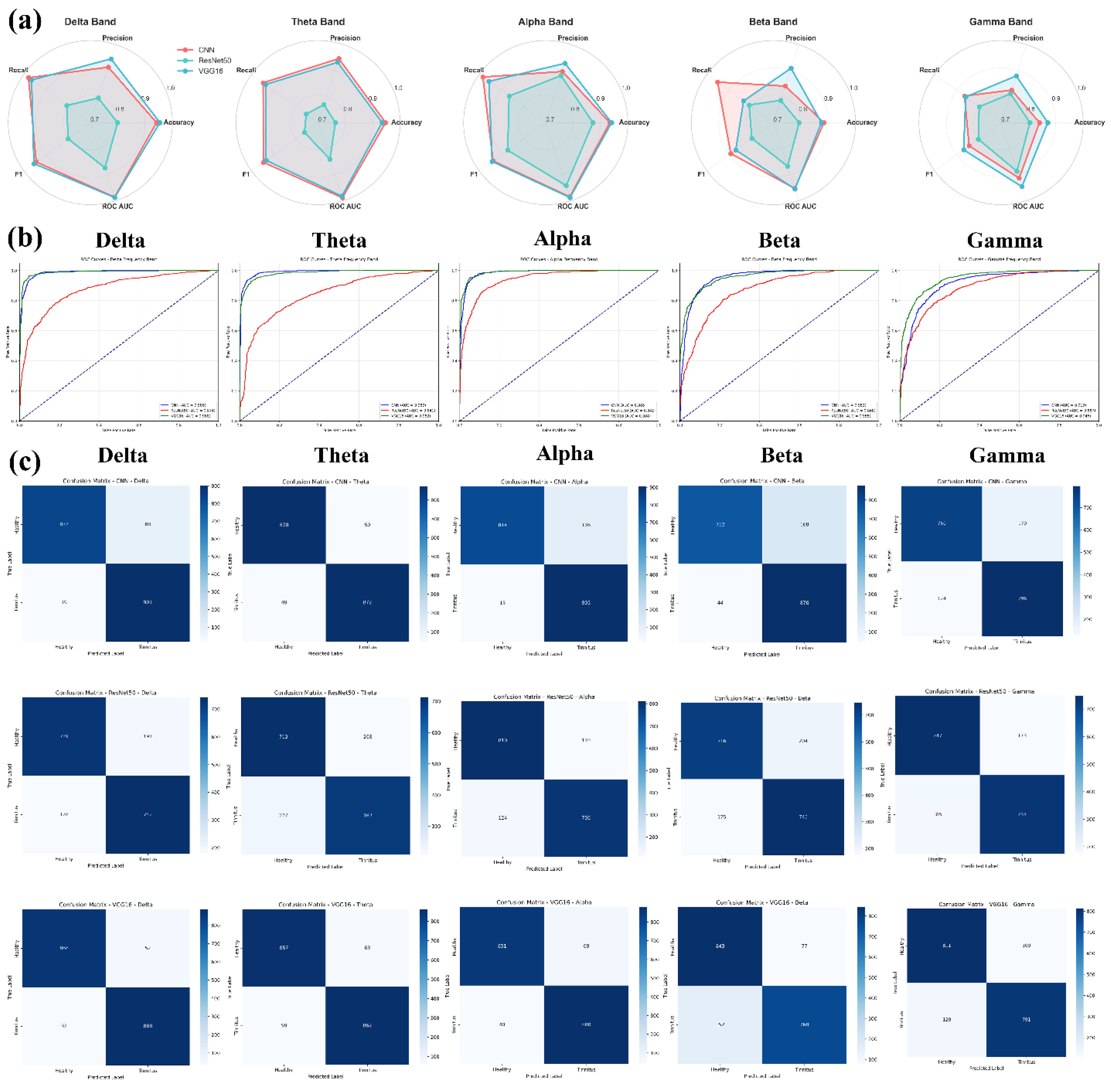
The comprehensive performance analysis reveals distinct patterns in model effectiveness across EEG frequency bands for tinnitus detection. VGG16 emerged as the most consistent performer, achieving the highest accuracies in Delta (95.4%), Theta (93.4%), and Alpha (94.1%) bands, with remarkably low standard deviations (0.009-0.024), indicating stable and reliable performance. CNN demonstrated competitive results with peak performance in the Theta band (94.7% accuracy) and maintained high recall values across all frequencies (>86%), suggesting strong sensitivity in detecting tinnitus cases. In contrast, ResNet50 showed the most variable performance, with accuracies ranging from 76.4% (Theta) to 87.3% (Alpha) and notably higher standard deviations, indicating less consistent classification outcomes.
3.7.2. Statistical Significance and Model Comparison
Statistical significance testing using DeLong's test revealed that CNN and VGG16 performed comparably across all frequency bands (p > 0.05), indicating no statistically significant differences in their discriminative capabilities. However, both CNN and VGG16 significantly outperformed ResNet50 in the Delta and Theta bands (p < 0.05), with CNN showing particularly strong superiority over ResNet50 in Delta (Z = 2.25, p = 0.024) and Theta (Z = 2.96, p = 0.003) frequencies. The Delta and Alpha frequency bands consistently yielded the highest classification performance across all models, with ROC AUC values exceeding 0.98 for VGG16 and CNN, while the Gamma band presented the most challenging classification task with the lowest overall accuracies (80.5-87.1%) and no significant differences between models. These findings suggest that low-frequency EEG components contain the most discriminative information for automated tinnitus detection using CWT-transformed neural network approaches, with CNN and VGG16 demonstrating equivalent and superior performance compared to ResNet50.
4. Discussion
This study analyzed 38 fMRI datasets (19 healthy, 19 tinnitus) and 80 EEG recordings (40 per group) to investigate neuroimaging biomarkers for tinnitus detection. The results demonstrated that CNN-based analysis of resting-state fMRI achieved optimal classification performance with slice 17 showing 99.0% ± 0.4% accuracy, representing the best-performing axial slice among 32 evaluated slices, while hybrid models combining pre-trained CNNs with traditional classifiers (VGG16-DT) reached 98.95% accuracy for automated tinnitus detection. EEG microstate analysis revealed systematic disruptions in neural network dynamics, with the most pronounced alterations observed in gamma-band microstate B occurrence rates (Cohen's d = 2.11, p = 1.58×10⁻¹⁴), where healthy participants exhibited significantly higher rates (56.56 vs 43.81 events/epoch). Additional significant microstate changes included reduced alpha-band microstate A coverage in both 4-state (34.62% vs 29.95%) and 6-state configurations, shortened microstate B durations in 5-state (1.23 vs 1.11 ms) and 7-state (1.12 vs 0.99 ms) configurations, and decreased beta-band microstate D durations in both 5-state (3.31 vs 2.93 ms) and 7-state (2.70 vs 2.34 ms) clustering solutions, collectively indicating that tinnitus pathophysiology involves widespread disruptions particularly affecting high-frequency gamma oscillations and alpha-band resting-state networks with altered temporal dynamics. Machine learning classification of EEG microstate features achieved up to 98.8% accuracy using Random Forest and Decision Tree algorithms, while CWT-transformed EEG analysis with deep learning models reached 95.4% accuracy, with delta and alpha frequency bands providing the most discriminative information for tinnitus detection.
Our findings demonstrate the effectiveness of neuroimaging approaches for automated tinnitus detection, examining fMRI and EEG modalities separately to establish their individual diagnostic capabilities. The superior performance of hybrid CNN models on rs-fMRI data (VGG16-Decision Tree: 98.95% accuracy) aligns with previous work by Xu et al. [21], who achieved 94.4% AUC using CNN on functional connectivity matrices from 200 participants. However, our study extends beyond connectivity analysis to direct slice-based classification, revealing spatial heterogeneity in discriminative capacity across brain regions, with mid-to-superior axial slices containing the most diagnostically relevant biomarkers. The EEG microstate analysis revealed systematic disruptions in tinnitus patients, particularly in gamma-band microstate B occurrence (Cohen's d = 2.11) and alpha-band coverage reductions, consistent with recent findings by Najafzadeh et al. [45], who reported significant alterations in beta and gamma band microstates with exceptional classification performance (100% accuracy in gamma band). Our results corroborate their findings regarding gamma-band importance while additionally demonstrating robust performance across multiple frequency bands using traditional machine learning approaches. The observed reductions in microstate durations and occurrence rates support the hypothesis of altered neural network dynamics in tinnitus, extending previous work by Jianbiao et al. [46], who identified increased sample entropy in δ, α2, and β1 bands using a smaller cohort (n=20). Our CWT-transformed EEG analysis using deep learning architectures yielded competitive results, with VGG16 achieving 95.4% accuracy in the Delta band. This approach differs from the innovative graph neural network methodology employed by Awais et al. [46], who achieved 99.41% accuracy by representing EEG channels as graph networks with GCN-LSTM architecture. While their graph-based approach showed superior single-metric performance, our multimodal framework provides broader clinical applicability through the integration of both structural (fMRI) and temporal (EEG) neural signatures. The novelty of our approach lies in the separate but comprehensive examination of both fMRI and EEG modalities, providing distinct insights into structural and temporal neural signatures of tinnitus. The spatially-specific fMRI slice analysis revealed heterogeneous discriminative patterns across brain regions, while frequency-specific EEG microstate characterization demonstrated systematic temporal disruptions. Unlike previous studies focusing on single modalities, our framework establishes that beta and alpha frequency bands contain the most discriminative EEG features, while specific fMRI slices corresponding to auditory processing regions show optimal diagnostic performance, each contributing unique diagnostic information. The consistent performance of tree-based classifiers (Random Forest, Decision Tree) across EEG features supports findings by Doborjeh et al. [47], who emphasized the importance of feature selection in achieving high classification accuracy (98-100%) for therapy outcome prediction. The clinical implications of our findings are substantial, with the high classification accuracies across multiple modalities suggesting potential for objective diagnostic tools in tinnitus assessment. The identification of specific neural signatures, particularly in gamma and alpha frequency bands, provides neurobiological insights that may inform therapeutic target identification and support the development of personalized treatment strategies.
The CNN performance analysis across 32 axial slices of rs-fMRI data (Figure 10) revealed spatial heterogeneity in discriminative capacity between tinnitus patients and healthy controls, with superior-to-middle axial slices demonstrating higher classification accuracy compared to inferior slices. Slices 17, 26, 14, 12, and 10 achieved accuracies exceeding 98%, while inferior slices (29, 32, 30, 31) showed lower discrimination with accuracies below 61%. This spatial gradient in classification performance aligns with neuroimaging findings demonstrating that superior temporal regions, particularly the superior temporal gyrus and primary auditory cortex, are involved in tinnitus pathophysiology [48]. Previous rs-fMRI studies have shown that tinnitus patients exhibit altered activity in superior temporal cortex regions, including the middle and superior temporal gyri, which corresponds to the higher performance of CNN models in middle-to-upper axial slices observed in our analysis. Furthermore, superior/middle temporal regions are involved in processing conflicts between auditory memory and signals from the peripheral auditory system, potentially explaining the discriminative capacity of these brain regions for tinnitus classification. The performance difference between superior (accuracy >98%) and inferior slices (accuracy <61%) suggests that tinnitus-associated neural alterations are spatially localized to specific anatomical regions, supporting the approach that analysis of superior temporal and auditory processing areas may provide relevant biomarkers for tinnitus assessment [49].
Figure 11a provides important insights into the altered neural dynamics observed in individuals with tinnitus by illustrating the spatial distribution of maximum voxel intensity differences across fMRI slices. The increased intensity variations found in the tinnitus group, especially in regions related to auditory processing and sensory integration, suggest disrupted neural activity that may be associated with the persistent perception of phantom sounds. These differences likely reflect mechanisms such as neural hyperactivity or maladaptive plasticity within the auditory cortex and its interconnected networks, both of which have been widely reported in the literature on tinnitus pathophysiology. In comparison, the more uniform patterns in healthy individuals indicate stable neural activity in the absence of such disturbances. The observed distribution of changes also suggests the involvement of non-auditory regions, including components of the limbic system, which may contribute to the emotional and cognitive experiences commonly reported in tinnitus [50]. These findings support the hypothesis that tinnitus involves not only abnormal auditory processing but also dysfunctional cross-modal and intra-auditory connectivity, reinforcing the presence of widespread alterations in brain networks. Figure 11b further highlights the differences in neural activity between healthy individuals and tinnitus patients through an analysis of mean voxel intensity values across axial fMRI slices. The consistently higher intensity values observed in the tinnitus group, particularly within slices 5 to 18 and 30 to 32, indicate abnormal neural dynamics that may be linked to increased activity and disrupted connectivity within critical auditory and non-auditory brain regions. These slices likely include structures such as the thalamus, auditory midbrain, and components of the limbic system, all of which play essential roles in auditory perception and the affective response to sound [51]. Additionally, the higher standard deviation of voxel intensity in the tinnitus group, reaching a value of 0.1572 in slice 31 compared to 0.0522 in the control group, suggests greater neural variability. This variability may reflect disrupted thalamocortical rhythms and maladaptive reorganization of brain activity [52]. Overall, these results reinforce the understanding that tinnitus is a condition involving widespread neural dysfunction. It affects not only the auditory pathways but also brain areas responsible for attention, emotional regulation, and multisensory integration [53]. The clear distinctions illustrated in Figure 11b align with previous neuroimaging studies reporting abnormal functional connectivity and increased activity within both auditory and limbic networks, providing additional support for the role of impaired neural synchronization in the manifestation of tinnitus.
The classification performance demonstrated in Figure 12 by hybrid models, particularly VGG16-DT (98.95% ± 2.94%), shows the effectiveness of combining pre-trained CNN feature extraction with traditional machine learning classifiers for neuroimaging-based tinnitus diagnosis. These results are consistent with recent developments in medical imaging where hybrid architectures have shown improved performance over standalone deep learning approaches by integrating automated feature extraction with interpretable classification mechanisms [45]. The performance across all models exceeding the 95% clinical relevance threshold, as illustrated in Figure 12, indicates the potential clinical utility of fMRI-based automated tinnitus detection, supporting previous observations that resting-state fMRI can distinguish tinnitus patients from healthy controls through altered neural connectivity patterns [21]. The superior performance of VGG16-based models over ResNet50 variants (98.76% vs. 97.94% average accuracy) may reflect VGG16's architectural suitability for capturing spatial patterns in brain imaging data, while the improved stability observed in hybrid approaches (particularly VGG16-RF with ±1.28% standard deviation) enhances the reliability necessary for clinical implementation. The average improvement of 1.2-2.8% in accuracy achieved by hybrid models over standalone CNNs indicates the value of integrating multiple algorithmic approaches, suggesting that the interpretability and robustness of traditional machine learning methods complement the feature extraction capabilities of deep neural networks in medical diagnostic applications.
The systematic disruptions in EEG microstate dynamics observed in our tinnitus cohort (Figure 13) provide evidence for neural network alterations underlying phantom auditory perception. The most pronounced finding, reduced gamma-band microstate occurrence rates (Cohen's d = 2.11, Table 9), aligns with established research demonstrating that gamma band activity in the auditory cortex correlates with tinnitus intensity and that decreased tinnitus loudness is associated with reduced gamma activity in auditory regions [54,55]. While previous studies have reported increased local gamma power in tinnitus patients, our findings suggest that global gamma-band network coordination is disrupted, reflecting maladaptive reorganization of auditory cortical networks that may contribute to the persistent phantom perception. The systematic reductions in alpha-band microstate parameters observed in our study (Figure 13, Table 9), including decreased coverage (29.95% vs 34.62%) and occurrence rates, are consistent with documented disruptions of default mode network connectivity in tinnitus patients and the established role of alpha oscillations in spatiotemporal organization of brain networks [56]. These alpha-band alterations likely reflect impaired resting-state network integrity, potentially underlying the intrusion of phantom auditory percepts into consciousness and the cognitive dysfunctions commonly associated with chronic tinnitus. The consistent beta-band microstate disruptions, including reduced coverage and shortened durations, align with neuroimaging evidence showing alterations in multiple resting-state networks in tinnitus patients, including attention networks and sensorimotor integration systems [49]. Our findings are further supported by recent research from Najafzadeh et al., who reported alterations in beta band microstates with increased microstate A duration and decreased microstate B duration in tinnitus patients, along with elevated occurrence rates in the tinnitus group [45]. The high statistical power (>0.99) and large effect sizes (Cohen's d = 1.08-2.34) across all frequency bands indicate clinically meaningful differences that collectively support the emerging conceptualization of tinnitus as a network disorder affecting multiple brain systems beyond the traditional auditory processing pathways [57].
The superior performance of tree-based algorithms, particularly Random Forest (RF) and Decision Tree (DT), achieving 98.8% accuracy with perfect precision (100.0%) for EEG microstate-based tinnitus classification (Figure 14, Table 10), aligns with recent findings demonstrating the effectiveness of ensemble methods in neurological disorder detection. These results are consistent with studies showing that Random Forest models excel in EEG-based tinnitus classification due to their robustness and ability to reduce overfitting while identifying key frequency band features [45]. The perfect precision achieved by RF and DT models indicates their reliability in minimizing false positive diagnoses, which is clinically relevant for avoiding unnecessary interventions. In contrast, the suboptimal performance of Deep Neural Networks (DNN) with 72.5% accuracy and high variability (±16.9%) suggests that traditional machine learning approaches may be more suitable for microstate feature classification in limited sample scenarios, a finding supported by research demonstrating processing speed advantages of tree-based methods over deep learning approaches [58]. The analysis of CWT-transformed EEG signals revealed distinct frequency-specific patterns, with VGG16 demonstrating the most consistent performance across Delta (95.4%), Theta (93.4%), and Alpha (94.1%) bands (Figure 16). The superior performance of low-frequency components (Delta and Alpha bands) with ROC AUC values exceeding 0.98 for CNN and VGG16 models supports previous research indicating that these frequency bands contain the most discriminative information for automated tinnitus detection [59]. The statistical validation using DeLong's test confirmed that while CNN and VGG16 performed comparably (p > 0.05), both significantly outperformed ResNet50 in Delta and Theta bands (p < 0.05), suggesting that simpler deep learning architectures may be more effective for EEG-based tinnitus classification than more complex models like ResNet50. These findings collectively demonstrate that both traditional machine learning approaches using microstate features and deep learning methods applied to frequency-transformed EEG data can achieve high classification accuracy, with the choice of method depending on the specific feature representation and computational requirements.
The present study employed parallel unimodal neuroimaging analyses to characterize tinnitus-related neural alterations using independent EEG and fMRI datasets obtained from separate cohorts. Although direct multimodal integration was not feasible, the convergent results across modalities offer complementary perspectives on tinnitus pathophysiology. In fMRI, the highest classification performance was observed in mid-to-superior axial slices, particularly slice 17, achieving 99.0% accuracy. This region corresponds to cortical areas encompassing the auditory cortex and functionally related association networks implicated in tinnitus generation [52]. This spatial localization aligns with previous neuroimaging evidence demonstrating aberrant functional connectivity within auditory and attention-related networks among tinnitus patients [60,61]. In parallel, EEG microstate analysis revealed significant alterations in high-frequency gamma oscillations (Cohen’s d = 2.11 for 7-state microstate B occurrence) and alpha-band network dynamics, consistent with electrophysiological findings of abnormal neural synchronization and resting-state instability in tinnitus [45,55]. The gamma-band abnormalities may reflect disrupted local cortical computations within regions corresponding to those identified by fMRI, as gamma oscillations are tightly linked to localized sensory and perceptual processing [62]. Moreover, the reduced alpha-band microstate coverage and duration observed in the EEG cohort mirror fMRI findings of altered connectivity within the default-mode and attentional networks [49,63]. Collectively, these parallel findings suggest that tinnitus involves both spatially localized disruptions in functional connectivity, detectable through hemodynamic imaging, and temporally dynamic instabilities in large-scale electrophysiological networks. Future investigations employing simultaneous EEG–fMRI acquisition in matched cohorts could directly examine the spatiotemporal coupling between these hemodynamic and electrophysiological alterations, thereby elucidating the mechanistic interplay between localized cortical dysfunction and distributed network reorganization in tinnitus pathophysiology [64,65].
In our fMRI analysis, individual time points were treated as independent observations to enable voxel-wise spatial pattern classification at fine temporal resolution. This methodological approach was motivated by emerging evidence supporting single-volume decoding frameworks that prioritize instantaneous spatial activation patterns over temporally aggregated connectivity metrics [66,67]. While conventional resting-state fMRI analyses typically compute functional connectivity through temporal correlations between brain regions [68], such approaches primarily capture static or time-averaged network interactions and may overlook transient spatial configurations that encode clinically relevant neurophysiological states [69]. The time-point-based classification framework employed here aligns with recent developments in dynamic pattern analysis and machine learning-based neuroimaging, where instantaneous spatial representations have demonstrated discriminative capacity for clinical phenotyping [70]. By analyzing individual volumes, our approach preserves spatial heterogeneity across axial slices and enables deep learning architectures to detect subtle regional activation patterns that may be obscured in connectivity matrices derived from temporal averaging [71]. The substantial sample size generated through this approach (400 time points per subject per slice) provided sufficient statistical power for the classifier to learn generalizable spatial biomarkers while accounting for temporal variability inherent in resting-state acquisitions [72]. We acknowledge that this methodology does not explicitly model temporal dependencies or dynamic functional connectivity fluctuations, which represent complementary dimensions of brain network organization [73]. Traditional connectivity-based approaches excel at characterizing inter-regional synchronization and network-level dysfunction [12], whereas our spatial pattern classification framework provides orthogonal information regarding localized activation signatures. These methodological paradigms should be viewed as complementary rather than mutually exclusive, each offering distinct insights into tinnitus-related neural alterations [74]. The high classification accuracy achieved through spatial pattern analysis (up to 99% for optimal slices) suggests that tinnitus manifests detectable spatial activation signatures independent of explicit temporal modeling, potentially reflecting sustained aberrant neural activity within specific cortical territories [75]. Future investigations will integrate temporal dynamics through hybrid architectures incorporating recurrent neural networks, long short-term memory units, or graph convolutional networks to jointly model spatiotemporal features [76], thereby providing a more comprehensive characterization of tinnitus-related network dysfunction. Additionally, combining time-point classification with sliding-window connectivity analysis and time-varying graph metrics would enable assessment of whether transient spatial patterns identified here correspond to specific dynamic functional connectivity states [77]. Such multimodal temporal-spatial integration would enhance both the biological interpretability and clinical utility of neuroimaging-based tinnitus biomarkers [78]. This slice-wise spatial classification approach is consistent with recent applications in other neuropsychiatric disorders, where similar time-point-based CNN methodologies achieved diagnostic accuracies exceeding 98% for schizophrenia detection using resting-state fMRI data, demonstrating the broader applicability of instantaneous spatial pattern analysis across clinical populations [79]. Such parallel findings across distinct clinical conditions support the validity of spatial decoding frameworks as complementary tools to traditional connectivity-based analyses in psychiatric neuroimaging.
The use of Global Field Power (GFP) as a spatial summary metric for subsequent time-frequency decomposition represents a deliberate methodological choice that balances computational efficiency with preservation of neurophysiologically relevant signal characteristics. While GFP collapses the 64-channel topographic distribution into a single time series representing the spatial standard deviation of scalp potentials at each time point, this metric specifically captures the overall strength of neural synchronization and global brain state dynamics that are independent of reference electrode selection [80]. Importantly, our analytical framework did not rely solely on GFP-derived features; the comprehensive microstate analysis explicitly preserved and analyzed topographic information through spatial clustering of multi-channel voltage distributions, extracting features including microstate duration, coverage, occurrence, and spatial configuration patterns across all 64 electrodes [35]. The GFP-to-CWT transformation was implemented as a complementary analysis stream designed to capture temporal dynamics of global neural synchronization within each frequency band, which has demonstrated particular relevance for characterizing aberrant neural oscillations in tinnitus pathophysiology [45]. This approach aligns with established frameworks in clinical neurophysiology where GFP serves as a robust marker of overall cortical excitability and network-level synchronization changes, particularly for detecting global alterations in brain state dynamics that characterize neuropsychiatric conditions [81]. The integration of both topographically-resolved microstate features (preserving spatial information) and GFP-derived time-frequency representations (emphasizing global synchronization dynamics) provided complementary perspectives on tinnitus-related neural alterations, with the former achieving 98.8% classification accuracy through spatial pattern analysis and the latter reaching 95.4% accuracy through temporal dynamics characterization. Future investigations will explore spatially-resolved time-frequency decomposition approaches, such as channel-wise CWT or source-space analysis, to integrate both spatial topography and temporal dynamics within unified multivariate representations [82].
All experiments were conducted on a system running Windows 11, equipped with an NVIDIA RTX 3050 Ti GPU, an Intel Core i7 processor, and 32 GB of RAM. The programming language used for model implementation was Python, with PyCharm as the integrated development environment (IDE). The deep learning models were developed and evaluated using the TensorFlow and Keras libraries, which provided a robust framework for neural network construction and training. Training times for each model varied significantly. The SVM required 2.025 hours, the RF took 4.63 hours, and the DT completed training in 0.335 hours. In comparison, the more complex DNN took 16.14 hours, and the CNN required 24.87 hours. These results reflect the trade-off between model complexity and computational efficiency.
Several methodological limitations must be acknowledged in interpreting these results. The EEG and fMRI datasets were derived from different participant cohorts, preventing direct multimodal feature integration and limiting our ability to leverage complementary information from both neuroimaging modalities. The fMRI data utilized publicly available datasets with male-only participants experiencing acoustic trauma-induced tinnitus, while EEG data were collected independently from mixed-etiology cohorts with balanced gender representation, resulting in potential differences in acquisition protocols, participant characteristics, and clinical assessment procedures that may affect direct comparisons between modalities. The fMRI dataset's restriction to male participants with acoustic trauma-induced tinnitus limits generalizability to the broader tinnitus population, particularly regarding gender-specific neural responses and non-acoustic etiologies. Furthermore, the different etiologies of tinnitus in our datasets may limit the generalizability of our findings, as acoustic trauma-induced tinnitus often involves specific cochlear damage patterns and may exhibit distinct neural signatures compared to tinnitus from other causes. The cross-sectional study design limits understanding of temporal stability of the identified neural biomarkers and their relationship to tinnitus symptom progression over time. Additionally, the relatively modest sample sizes (40 per group for EEG, 19 per group for fMRI) may limit generalizability across different tinnitus subtypes, severity levels, and demographic populations.
Future investigations should prioritize the collection of matched EEG and fMRI data from identical participant cohorts to enable true multimodal analysis and feature fusion approaches that could potentially improve classification accuracy and provide more comprehensive characterization of tinnitus-related neural alterations. Validation across diverse tinnitus etiologies will be essential to ensure broad clinical applicability of these classification approaches. Longitudinal studies tracking patients over extended periods would help establish the temporal stability of identified biomarkers and their potential utility for monitoring treatment response. The development of real-time processing algorithms and optimization of computational requirements will be essential for clinical translation, along with validation studies across multiple clinical centers using standardized protocols. Integration of additional clinical measures, including detailed tinnitus severity assessments, audiological profiles, and psychological evaluations, would enhance the clinical relevance of these neuroimaging-based classification approaches and support the development of personalized treatment strategies based on individual neural signatures.
The high classification accuracies achieved in this study (98.8% for EEG microstate analysis and 98.95% for fMRI hybrid models) suggest potential clinical utility for objective tinnitus diagnosis. However, successful clinical implementation requires addressing several practical considerations including integration with existing audiological workflows, establishment of standardized acquisition protocols across different clinical centers, and development of user-friendly interfaces for non-technical clinical staff. The computational requirements and processing times observed in our study (ranging from 0.335 to 24.87 hours depending on the model) indicate the need for optimized implementations and appropriate hardware infrastructure in clinical settings. Furthermore, regulatory approval pathways for AI-based diagnostic tools will require validation on larger, more diverse patient populations and demonstration of consistent performance across different scanner types and acquisition parameters.
The identification of objective neural biomarkers for tinnitus represents a significant advancement toward evidence-based diagnosis and treatment monitoring in a condition that has traditionally relied on subjective patient reports. The high classification accuracies achieved across both neuroimaging modalities suggest potential for reducing diagnostic uncertainty and supporting clinical decision-making, particularly in cases where symptom presentation is ambiguous or when objective assessment is required for research or medico-legal purposes. The specific neural signatures identified, particularly in gamma and alpha frequency bands, may inform the development of targeted therapeutic interventions, including neurofeedback protocols and brain stimulation approaches. However, successful clinical implementation will require careful consideration of cost-effectiveness, training requirements for clinical staff, and integration with existing healthcare infrastructure to ensure broad accessibility and practical utility in routine clinical practice.
Taken together, the findings from this study underscore the complementary strengths of EEG and fMRI in elucidating tinnitus-related neural mechanisms. The EEG analyses captured the rapid temporal fluctuations and network instabilities underlying abnormal oscillatory dynamics, whereas the fMRI analyses identified spatially localized alterations in auditory and attentional cortical regions. The convergence of these independent observations supports the hypothesis that tinnitus arises from both localized cortical hyperactivity and disrupted large-scale network coordination. By establishing a comparative framework that integrates temporal and spatial perspectives, this work advances the understanding of tinnitus pathophysiology and highlights the value of multi-perspective neuroimaging for developing objective diagnostic biomarkers. Future research should extend this framework using simultaneous EEG–fMRI acquisition and larger, matched cohorts to directly examine the spatiotemporal interactions between electrophysiological and hemodynamic activity in tinnitus, ultimately paving the way toward personalized and mechanism-based therapeutic interventions.
5. Conclusion
This study demonstrated the potential of advanced machine learning and deep learning approaches for neuroimaging-based tinnitus classification using independent EEG and fMRI datasets. The EEG microstate analysis achieved 98.8% classification accuracy, while the hybrid fMRI framework integrating VGG16 with Decision Tree classifiers reached 98.95% accuracy. Across 80 EEG recordings and 38 fMRI datasets, tinnitus patients exhibited consistent neural alterations, including pronounced gamma-band microstate disruptions (Cohen’s d = 2.11) and reduced alpha-band coverage, indicating dysregulated oscillatory dynamics. The fMRI analysis further identified 12 high-performing axial slices out of 32 evaluated, with slice 17 showing optimal accuracy (99.0% ± 0.4%), reflecting spatially localized functional connectivity abnormalities associated with tinnitus. Collectively, these findings highlight the complementary strengths of EEG and fMRI in capturing temporally dynamic and spatially specific neural signatures of tinnitus and underscore the diagnostic potential of hybrid and tree-based algorithms for objective neuroimaging assessment.
Despite these promising results, several methodological and translational considerations remain. The use of independent EEG and fMRI cohorts in this study precluded direct multimodal feature integration, emphasizing the need for future investigations employing matched datasets to enable true multimodal analysis. Standardization of imaging protocols, validation across diverse tinnitus etiologies, and the development of scalable computational frameworks will be essential for clinical translation. Moreover, integrating detailed audiological and psychological assessments could enhance the clinical interpretability of these neuroimaging-derived biomarkers. The identification of robust neural signatures, particularly in gamma and alpha frequency bands, provides a foundation for future longitudinal and multimodal studies aimed at developing personalized, mechanism-based diagnostic and therapeutic strategies for tinnitus.
Author Contributions
H.N. conceived and supervised the study, ensuring scientific integrity, methodological rigor, and overall project coordination. K.K. led the EEG and fMRI data analysis pipeline, including signal preprocessing, microstate segmentation, feature extraction, and development of machine learning and deep learning models. K.K also designed the hybrid classification architecture and contributed extensively to performance evaluation and visualization. S.S. provided clinical expertise in tinnitus, contributed to patient selection criteria for the EEG dataset, and offered medical interpretation of the neurophysiological findings to ensure clinical relevance of the results. K.K. and S.S. jointly curated the EEG dataset and ensured consistency between clinical characteristics and neuroimaging data. S.E. implemented the classification algorithms, carried out statistical analyses, and assisted in EEG signal processing. A.J. supported deep learning model optimization and validation, particularly in the multimodal fusion stage. F.Sh. contributed to performance benchmarking, technical troubleshooting, and critical review of analytical procedures. The initial manuscript draft was prepared by K.K. and S.E., and extensively revised and refined by H.N., A.J., and F.Sh. to ensure scientific clarity and coherence. All authors participated in result interpretation, provided constructive feedback, and approved the final version of the manuscript.
Funding
The authors received no specific funding for this work.
Data Availability
The fMRI dataset utilized in this study is publicly accessible at:
https://openneuro.org/datasets/ds002896/versions/1.0.0/download. The EEG dataset supporting the findings of
this study is not publicly available. However, it can be obtained upon reasonable request from the corresponding
author.
Acknowledgments
The authors would like to thank the open-source community and OpenNeuro for providing access to the fMRI datasets used in this research. We also extend our gratitude to all participants who contributed to the EEG data collection. Additionally, the authors would like to acknowledge the Iranian National Brain Mapping Laboratory (NBML), Tehran, Iran, for providing data acquisition (analysis) services for this research work.
Competing interests
The authors declare no competing interests.
Declarations:
All experimental protocols were approved by the Ethics Committee of Tabriz University of Medical Sciences, Tabriz, Iran, in accordance with the principles of the Declaration of Helsinki.
References
- A. McCormack et al., "The prevalence of tinnitus and the relationship with neuroticism in a middle-aged UK population," Journal of Psychosomatic Research, vol. 76, no. 1, pp. 56-60, 2014. [CrossRef]
- J. M. Bhatt, N. Bhattacharyya, and H. W. Lin, "Relationships between tinnitus and the prevalence of anxiety and depression," The laryngoscope, vol. 127, no. 2, pp. 466-469, 2017. [CrossRef]
- F. Ramezani and H. Bolhasani, "A Review on the Applications of Machine Learning for Tinnitus Diagnosis Using EEG Signals," arXiv preprint arXiv:2310.18795, 2023.
- T. Manabe et al., "EEG topographic features for assessing skill levels during laparoscopic surgical training," 2022.
- K. Kim, N. T. Duc, M. Choi, and B. Lee, "EEG microstate features for schizophrenia classification," PloS one, vol. 16, no. 5, p. e0251842, 2021. [CrossRef]
- M. Rahmati, A. Jalaeianbanayan, J. Vahedi, H. Najafzadeh, and B. Danesh, "Novel EEG-based diagnostic framework for Major Depressive Disorder using microstate and entropy features," Cognitive Neurodynamics, vol. 19, no. 1, p. 116, 2025. [CrossRef]
- P. S. Moghaddam, A. Vaziri, S. S. Khatami, F. Hernando-Gallego, and D. Martín, "Generative Adversarial and Transformer Network Synergy for Robust Intrusion Detection in IoT Environments," Future Internet, vol. 17, no. 6, p. 258, 2025. [CrossRef]
- A. Salehiyan, P. S. Moghaddam, and M. Kaveh, "An Optimized Transformer–GAN–AE for Intrusion Detection in Edge and IIoT Systems: Experimental Insights from WUSTL-IIoT-2021, EdgeIIoTset, and TON_IoT Datasets," Future Internet, vol. 17, no. 7, p. 279, 2025. [CrossRef]
- A. Vaziri, P. S. Moghaddam, M. Shoeibi, and M. Kaveh, "Energy-Efficient Secure Cell-Free Massive MIMO for Internet of Things: A Hybrid CNN–LSTM-Based Deep-Learning Approach," Future Internet, vol. 17, no. 4, p. 169, 2025. [CrossRef]
- Z. Raeisi, O. Bashiri, M. EskandariNasab, M. Arshadi, A. Golkarieh, and H. Najafzadeh, "EEG microstate biomarkers for schizophrenia: a novel approach using deep neural networks," Cognitive Neurodynamics, vol. 19, no. 1, pp. 1-26, 2025.
- Z. Raeisi, R. A. Lashaki, F. Sharafkhani, A. Roshanzamir, and H. Najafzadeh, "Enhanced Classification of Tinnitus Patients Using EEG Microstates and Deep Learning Techniques," 2024. [CrossRef]
- E.-S. Hong, H.-S. Kim, S. K. Hong, D. Pantazis, and B.-K. Min, "Deep learning-based electroencephalic diagnosis of tinnitus symptom," Frontiers in Human Neuroscience, vol. 17, p. 1126938, 2023. [CrossRef]
- M. Saeidi et al., "Neural decoding of EEG signals with machine learning: a systematic review," Brain Sciences, vol. 11, no. 11, p. 1525, 2021. [CrossRef]
- S. Agrawal, V. Chinnadurai, and R. Sharma, "Hemodynamic functional connectivity optimization of frequency EEG microstates enables attention LSTM framework to classify distinct temporal cortical communications of different cognitive tasks," Brain Informatics, vol. 9, no. 1, p. 25, 2022. [CrossRef]
- A. Keihani, S. S. Sajadi, M. Hasani, and F. Ferrarelli, "Bayesian optimization of machine learning classification of resting-state EEG microstates in schizophrenia: a proof-of-concept preliminary study based on secondary analysis," Brain Sciences, vol. 12, no. 11, p. 1497, 2022. [CrossRef]
- A. Piarulli et al., "Tinnitus and distress: an electroencephalography classification study," Brain communications, vol. 5, no. 1, p. fcad018, 2023. [CrossRef]
- X. Ma, F. Wang, C. Zhang, W. Shen, and S. Yang, "Self-Directed Neurofeedback Treatment for Subjective Tinnitus Patients Evaluated by Multimodal Functional Imaging," Neural Plasticity, vol. 2022, no. 1, p. 5114721, 2022. [CrossRef]
- M. Rashid, H. Singh, and V. Goyal, "The use of machine learning and deep learning algorithms in functional magnetic resonance imaging—A systematic review," Expert Systems, vol. 37, no. 6, p. e12644, 2020.
- Y. Cao, M. Lu, J. Fu, Z. Guo, and Z. Gao, "Identifying Alzheimer’s disease from 4D fMRI using hybrid 3DCNN and GRU networks," in Fourteenth International Conference on Digital Image Processing (ICDIP 2022), 2022, vol. 12342: SPIE, pp. 379-385.
- C.-T. Lin et al., "Multi-tasking deep network for tinnitus classification and severity prediction from multimodal structural MR images," Journal of neural engineering, vol. 20, no. 1, p. 016017, 2023. [CrossRef]
- Q. Xu et al., "Tinnitus classification based on resting-state functional connectivity using a convolutional neural network architecture," Neuroimage, vol. 290, p. 120566, 2024. [CrossRef]
- G. Xu et al., "A deep transfer convolutional neural network framework for EEG signal classification," IEEE Access, vol. 7, pp. 112767-112776, 2019.
- A. Job, A. Kavounoudias, C. Jaroszynski, A. Jaillard, and C. Delon-Martin, "Specific connectivity with Operculum 3 (OP3) brain region in acoustic trauma tinnitus: a seed-based resting state fMRI study," bioRxiv, p. 676429, 2019.
- W. Klimesch, "EEG alpha and theta oscillations reflect cognitive and memory performance: a review and analysis," Brain research reviews, vol. 29, no. 2-3, pp. 169-195, 1999. [CrossRef]
- A. Delorme and S. Makeig, "EEGLAB: an open source toolbox for analysis of single-trial EEG dynamics including independent component analysis," Journal of neuroscience methods, vol. 134, no. 1, pp. 9-21, 2004. [CrossRef]
- A. K. Jain, Fundamentals of digital image processing. Prentice-Hall, Inc., 1989.
- K. Zuiderveld, "Contrast limited adaptive histogram equalization," in Graphics gems IV, 1994, pp. 474-485.
- J. D. Power, K. A. Barnes, A. Z. Snyder, B. L. Schlaggar, and S. E. Petersen, "Spurious but systematic correlations in functional connectivity MRI networks arise from subject motion," Neuroimage, vol. 59, no. 3, pp. 2142-2154, 2012.
- M. Jenkinson, P. Bannister, M. Brady, and S. Smith, "Improved optimization for the robust and accurate linear registration and motion correction of brain images," Neuroimage, vol. 17, no. 2, pp. 825-841, 2002. [CrossRef]
- S. D. Muthukumaraswamy, "High-frequency brain activity and muscle artifacts in MEG/EEG: a review and recommendations," Frontiers in human neuroscience, vol. 7, p. 138, 2013.
- A. J. Shackman, B. W. McMenamin, J. S. Maxwell, L. L. Greischar, and R. J. Davidson, "Identifying robust and sensitive frequency bands for interrogating neural oscillations," Neuroimage, vol. 51, no. 4, pp. 1319-1333, 2010. [CrossRef]
- I. I. Goncharova, D. J. McFarland, T. M. Vaughan, and J. R. Wolpaw, "EMG contamination of EEG: spectral and topographical characteristics," Clinical neurophysiology, vol. 114, no. 9, pp. 1580-1593, 2003. [CrossRef]
- S. Yuval-Greenberg, O. Tomer, A. S. Keren, I. Nelken, and L. Y. Deouell, "Transient induced gamma-band response in EEG as a manifestation of miniature saccades," Neuron, vol. 58, no. 3, pp. 429-441, 2008. [CrossRef]
- H. Nolan, R. Whelan, and R. B. Reilly, "FASTER: fully automated statistical thresholding for EEG artifact rejection," Journal of neuroscience methods, vol. 192, no. 1, pp. 152-162, 2010.
- C. M. Michel and T. Koenig, "EEG microstates as a tool for studying the temporal dynamics of whole-brain neuronal networks: a review," Neuroimage, vol. 180, pp. 577-593, 2018. [CrossRef]
- P. T. Zebhauser, V. D. Hohn, and M. Ploner, "Resting state EEG and MEG as biomarkers of chronic pain: A systematic review," Pain, p. 10.1097, 2022.
- D. Lehmann and W. Skrandies, "Reference-free identification of components of checkerboard-evoked multichannel potential fields," Electroencephalography and clinical neurophysiology, vol. 48, no. 6, pp. 609-621, 1980. [CrossRef]
- Y. LeCun, Y. Bengio, and G. Hinton, "Deep learning," nature, vol. 521, no. 7553, pp. 436-444, 2015.
- C. Cortes and V. Vapnik, "Support-vector networks," Machine learning, vol. 20, pp. 273-297, 1995.
- L. Breiman, "Random forests," Machine learning, vol. 45, pp. 5-32, 2001.
- S. R. Safavian and D. Landgrebe, "A survey of decision tree classifier methodology," IEEE transactions on systems, man, and cybernetics, vol. 21, no. 3, pp. 660-674, 1991. [CrossRef]
- K. Simonyan and A. Zisserman, "Very deep convolutional networks for large-scale image recognition," arXiv preprint arXiv:1409.1556, 2014.
- K. He, X. Zhang, S. Ren, and J. Sun, "Deep residual learning for image recognition," in Proceedings of the IEEE conference on computer vision and pattern recognition, 2016, pp. 770-778.
- W. Zhu, N. Zeng, and N. Wang, "Sensitivity, specificity, accuracy, associated confidence interval and ROC analysis with practical SAS implementations," NESUG proceedings: health care and life sciences, Baltimore, Maryland, vol. 19, p. 67, 2010.
- Z. Raeisi et al., "Enhanced classification of tinnitus patients using EEG microstates and deep learning techniques," Scientific Reports, vol. 15, no. 1, p. 15959, 2025. [CrossRef]
- M. Jianbiao, W. Xinzui, L. Zhaobo, L. Juan, Z. Zhongwei, and F. Hui, "EEG signal classification of tinnitus based on SVM and sample entropy," Computer Methods in Biomechanics and Biomedical Engineering, vol. 26, no. 5, pp. 580-594, 2023. [CrossRef]
- M. Doborjeh et al., "Prediction of tinnitus treatment outcomes based on EEG sensors and TFI score using deep learning," Sensors, vol. 23, no. 2, p. 902, 2023. [CrossRef]
- A. M. Leaver, L. Renier, M. A. Chevillet, S. Morgan, H. J. Kim, and J. P. Rauschecker, "Dysregulation of limbic and auditory networks in tinnitus," Neuron, vol. 69, no. 1, pp. 33-43, 2011. [CrossRef]
- S. A. Schmidt, K. Akrofi, J. R. Carpenter-Thompson, and F. T. Husain, "Default mode, dorsal attention and auditory resting state networks exhibit differential functional connectivity in tinnitus and hearing loss," PloS one, vol. 8, no. 10, p. e76488, 2013. [CrossRef]
- W.-W. Cai, Z.-c. Li, Q.-t. Yang, and T. Zhang, "Abnormal spontaneous neural activity of the central auditory system changes the functional connectivity in the tinnitus brain: a resting-state functional MRI study," Frontiers in neuroscience, vol. 13, p. 1314, 2019. [CrossRef]
- F. T. Husain and S. A. Schmidt, "Using resting state functional connectivity to unravel networks of tinnitus," Hearing research, vol. 307, pp. 153-162, 2014. [CrossRef]
- W. Schlee, N. Weisz, O. Bertrand, T. Hartmann, and T. Elbert, "Using auditory steady state responses to outline the functional connectivity in the tinnitus brain," PLoS One, vol. 3, no. 11, p. e3720, 2008. [CrossRef]
- D. De Ridder, S. Vanneste, B. Langguth, and R. Llinas, "Thalamocortical dysrhythmia: a theoretical update in tinnitus," Frontiers in neurology, vol. 6, p. 124, 2015. [CrossRef]
- E. van Der Loo et al., "Tinnitus intensity dependent gamma oscillations of the contralateral auditory cortex," PloS one, vol. 4, no. 10, p. e7396, 2009.
- N. Weisz, S. Moratti, M. Meinzer, K. Dohrmann, and T. Elbert, "Tinnitus perception and distress is related to abnormal spontaneous brain activity as measured by magnetoencephalography," PLoS medicine, vol. 2, no. 6, p. e153, 2005. [CrossRef]
- S. Rosemann and J. P. Rauschecker, "Disruptions of default mode network and precuneus connectivity associated with cognitive dysfunctions in tinnitus," Scientific Reports, vol. 13, no. 1, p. 5746, 2023.
- B.Langguth, P. M. Kreuzer, T. Kleinjung, and D. De Ridder, "Tinnitus: causes and clinical management," The Lancet Neurology, vol. 12, no. 9, pp. 920-930, 2013. [CrossRef]
- P. S. Shabestari et al., "Prediction of acoustic tinnitus suppression using resting-state EEG via explainable AI approach," Scientific Reports, vol. 15, no. 1, p. 10968, 2025. [CrossRef]
- R. T. Schirrmeister et al., "Deep learning with convolutional neural networks for EEG decoding and visualization," Human brain mapping, vol. 38, no. 11, pp. 5391-5420, 2017. [CrossRef]
- F. T. Husain et al., "Neuroanatomical changes due to hearing loss and chronic tinnitus: a combined VBM and DTI study," Brain research, vol. 1369, pp. 74-88, 2011. [CrossRef]
- Y.-C. Chen et al., "Aberrant spontaneous brain activity in chronic tinnitus patients revealed by resting-state functional MRI," NeuroImage: Clinical, vol. 6, pp. 222-228, 2014. [CrossRef]
- P. Fries, "Neuronal gamma-band synchronization as a fundamental process in cortical computation," Annual review of neuroscience, vol. 32, no. 1, pp. 209-224, 2009. [CrossRef]
- S. Vanneste and D. De Ridder, "The auditory and non-auditory brain areas involved in tinnitus. An emergent property of multiple parallel overlapping subnetworks," Frontiers in systems neuroscience, vol. 6, p. 31, 2012.
- D. De Ridder et al., "An integrative model of auditory phantom perception: tinnitus as a unified percept of interacting separable subnetworks," Neuroscience & Biobehavioral Reviews, vol. 44, pp. 16-32, 2014.
- D. Lehmann, R. D. Pascual-Marqui, W. K. Strik, and T. Koenig, "Core networks for visual-concrete and abstract thought content: a brain electric microstate analysis," Neuroimage, vol. 49, no. 1, pp. 1073-1079, 2010.
- J. V. Haxby, A. C. Connolly, and J. S. Guntupalli, "Decoding neural representational spaces using multivariate pattern analysis," Annual review of neuroscience, vol. 37, no. 1, pp. 435-456, 2014. [CrossRef]
- R. A. Poldrack, G. Huckins, and G. Varoquaux, "Establishment of best practices for evidence for prediction: a review," JAMA psychiatry, vol. 77, no. 5, pp. 534-540, 2020. [CrossRef]
- B. Biswal, F. Zerrin Yetkin, V. M. Haughton, and J. S. Hyde, "Functional connectivity in the motor cortex of resting human brain using echo-planar MRI," Magnetic resonance in medicine, vol. 34, no. 4, pp. 537-541, 1995. [CrossRef]
- E. A. Allen, E. Damaraju, S. M. Plis, E. B. Erhardt, T. Eichele, and V. D. Calhoun, "Tracking whole-brain connectivity dynamics in the resting state," Cerebral cortex, vol. 24, no. 3, pp. 663-676, 2014. [CrossRef]
- S. Vieira, W. H. Pinaya, and A. Mechelli, "Using deep learning to investigate the neuroimaging correlates of psychiatric and neurological disorders: Methods and applications," Neuroscience & Biobehavioral Reviews, vol. 74, pp. 58-75, 2017. [CrossRef]
- M. Khosla, K. Jamison, G. H. Ngo, A. Kuceyeski, and M. R. Sabuncu, "Machine learning in resting-state fMRI analysis," Magnetic resonance imaging, vol. 64, pp. 101-121, 2019. [CrossRef]
- G. Varoquaux, "Cross-validation failure: Small sample sizes lead to large error bars," Neuroimage, vol. 180, pp. 68-77, 2018.
- D. J. Lurie et al., "Questions and controversies in the study of time-varying functional connectivity in resting fMRI," Network neuroscience, vol. 4, no. 1, pp. 30-69, 2020. [CrossRef]
- E. Tagliazucchi and H. Laufs, "Decoding wakefulness levels from typical fMRI resting-state data reveals reliable drifts between wakefulness and sleep," Neuron, vol. 82, no. 3, pp. 695-708, 2014. [CrossRef]
- Y. C. Chen et al., "Tinnitus distress is linked to enhanced resting-state functional connectivity from the limbic system to the auditory cortex," Human brain mapping, vol. 38, no. 5, pp. 2384-2397, 2017. [CrossRef]
- S. Wang, H. Wang, Y. Shen, and X. Wang, "Automatic recognition of mild cognitive impairment and alzheimers disease using ensemble based 3d densely connected convolutional networks," in 2018 17th IEEE International conference on machine learning and applications (ICMLA), 2018: IEEE, pp. 517-523.
- S. Shakil, C.-H. Lee, and S. D. Keilholz, "Evaluation of sliding window correlation performance for characterizing dynamic functional connectivity and brain states," Neuroimage, vol. 133, pp. 111-128, 2016. [CrossRef]
- C.-W. Woo, L. J. Chang, M. A. Lindquist, and T. D. Wager, "Building better biomarkers: brain models in translational neuroimaging," Nature neuroscience, vol. 20, no. 3, pp. 365-377, 2017. [CrossRef]
- Z. Raeisi, M. Mehrnia, R. Ahmadi Lashaki, and F. Abedi Lomer, "Enhancing schizophrenia diagnosis through deep learning: a resting-state fMRI approach," Neural Computing and Applications, pp. 1-33, 2025.
- W. Skrandies, "Global field power and topographic similarity," Brain topography, vol. 3, no. 1, pp. 137-141, 1990. [CrossRef]
- A. Khanna, A. Pascual-Leone, C. M. Michel, and F. Farzan, "Microstates in resting-state EEG: current status and future directions," Neuroscience & Biobehavioral Reviews, vol. 49, pp. 105-113, 2015. [CrossRef]
- M. X. Cohen, Analyzing neural time series data: theory and practice. MIT press, 2014.
Figure 1.
An Example of Filtered EEG Signals for One Second: Original and Band-Pass Filtered Signals in Delta, Theta, Alpha, Beta, and Gamma Bands Across Healthy and Tinnitus Groups.
Figure 1.
An Example of Filtered EEG Signals for One Second: Original and Band-Pass Filtered Signals in Delta, Theta, Alpha, Beta, and Gamma Bands Across Healthy and Tinnitus Groups.
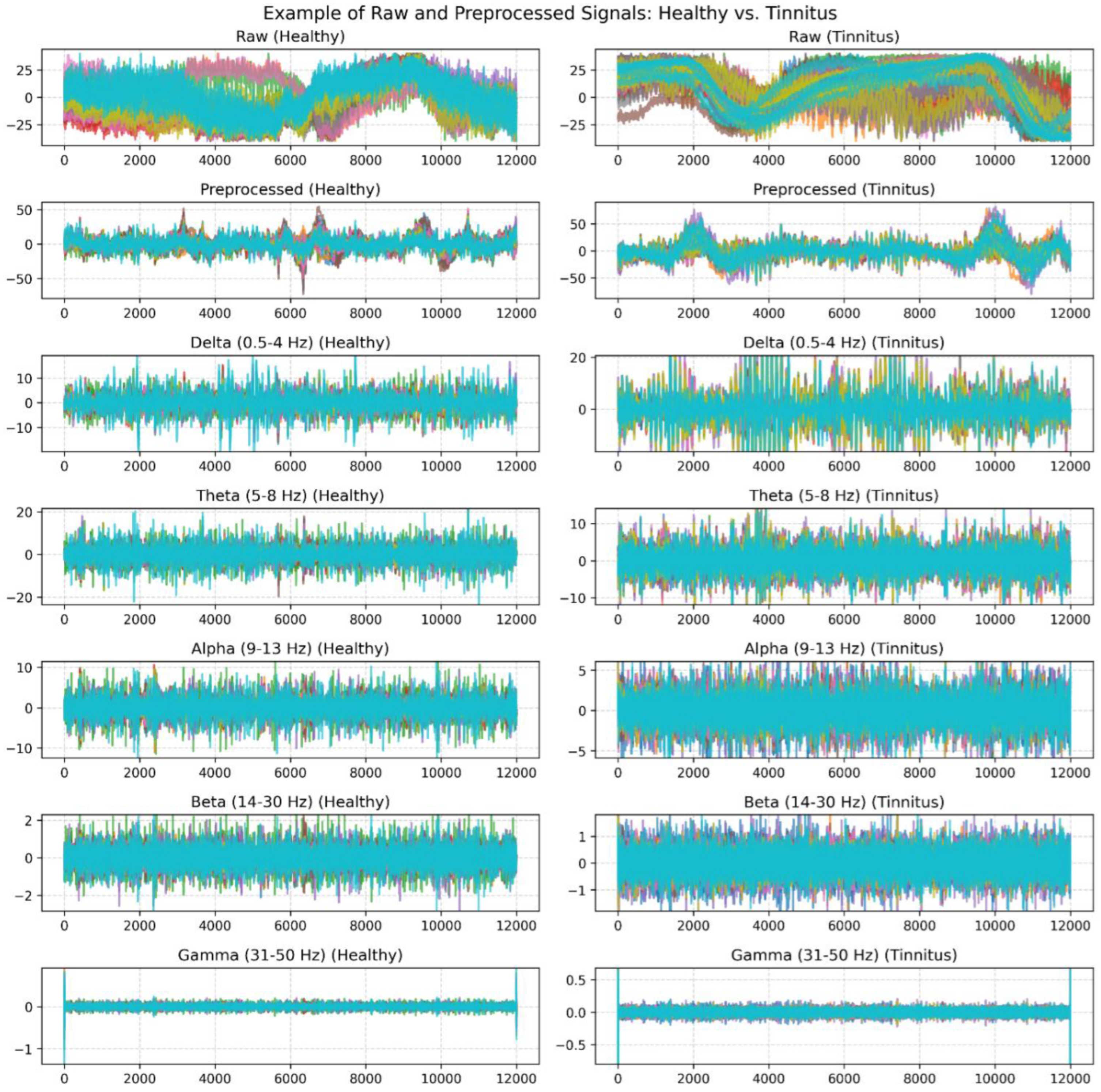
Figure 2.
Comparison of Raw and Improved rs-fMRI Images After Image Enhancement Operations.
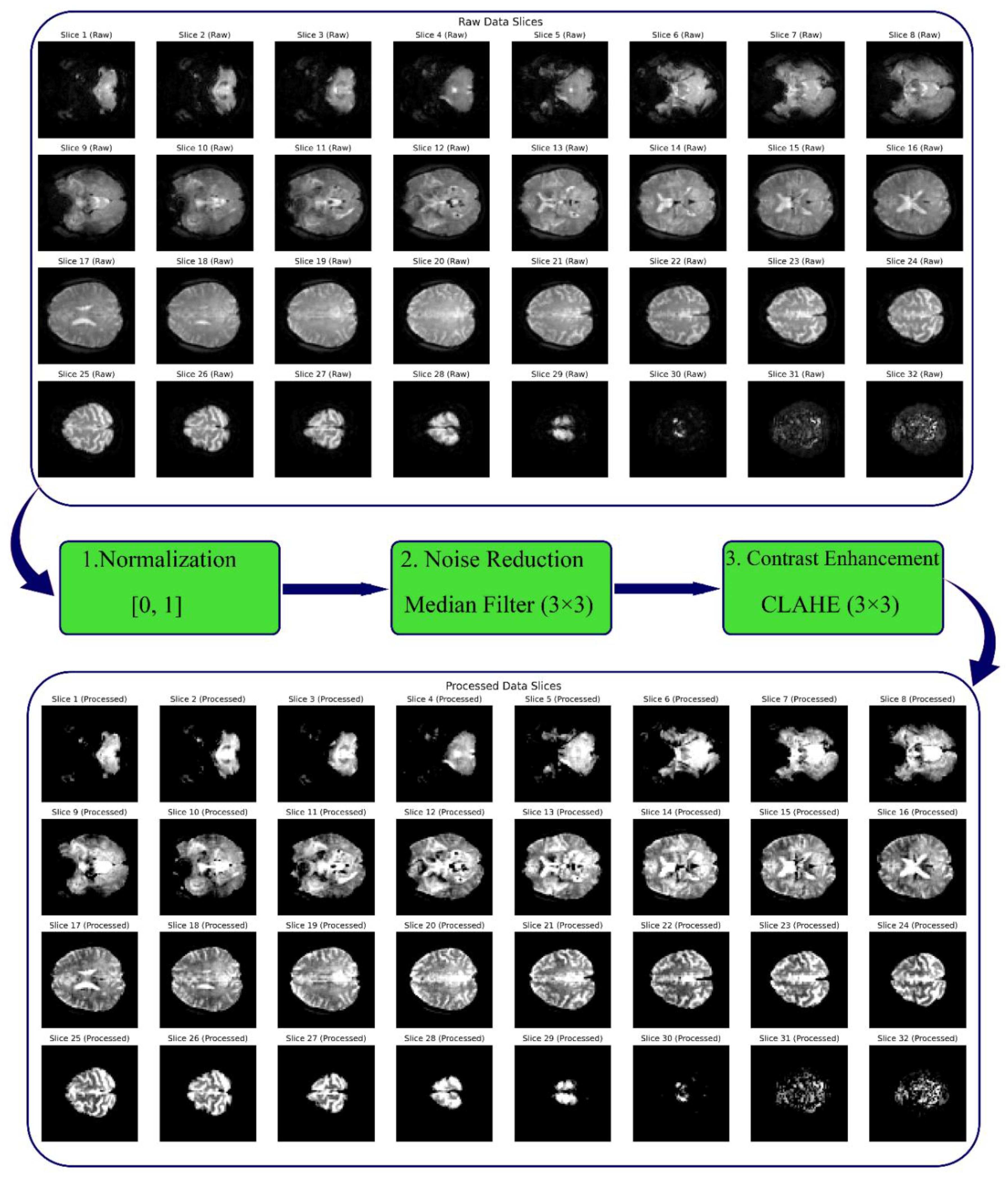
Figure 3.
Sample of EEG Signal in the Alpha Band, Topographic Clustering, and Global Field Power (GFP).
Figure 3.
Sample of EEG Signal in the Alpha Band, Topographic Clustering, and Global Field Power (GFP).
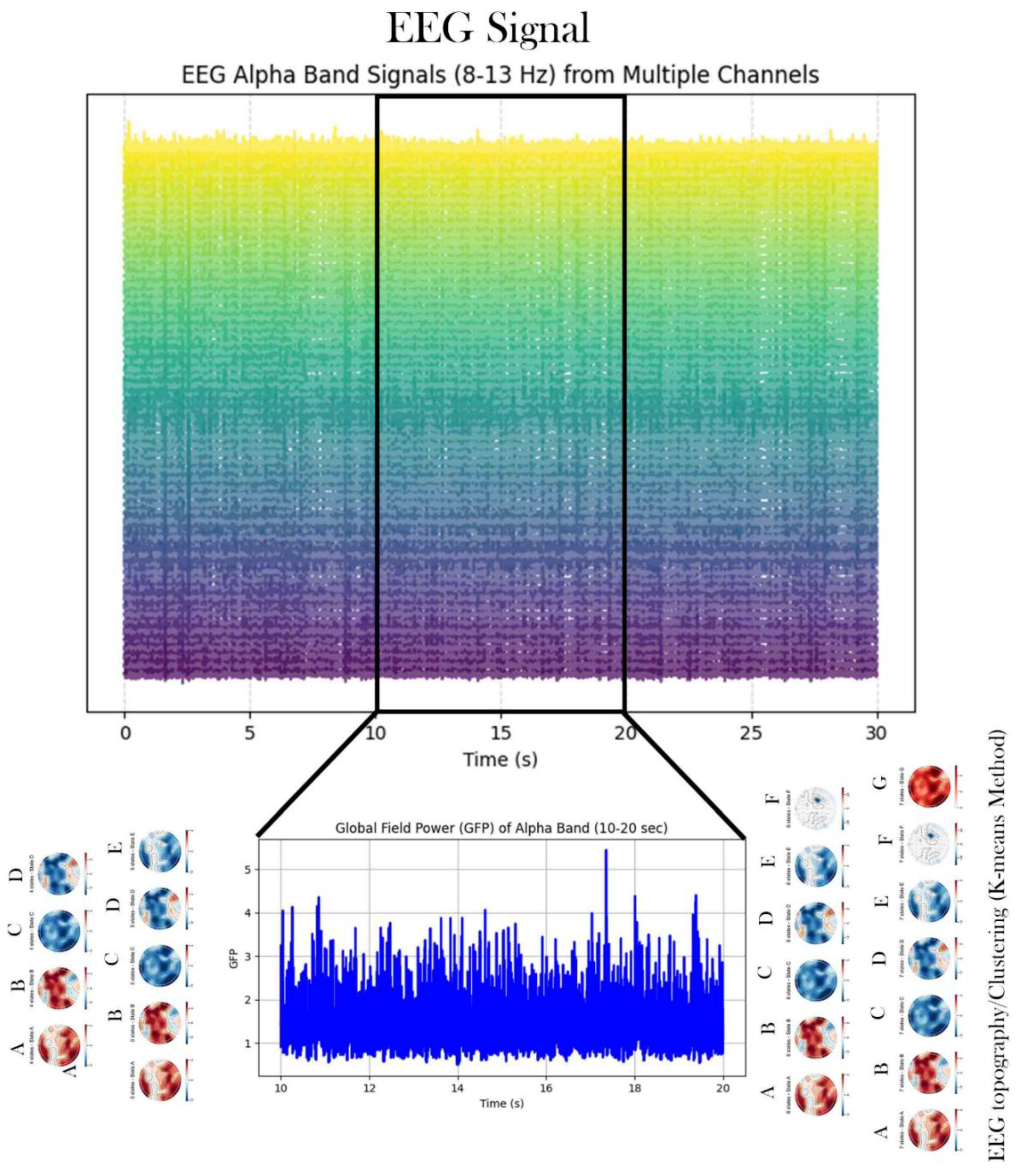
Figure 5.
Architecture of a CNN Model.
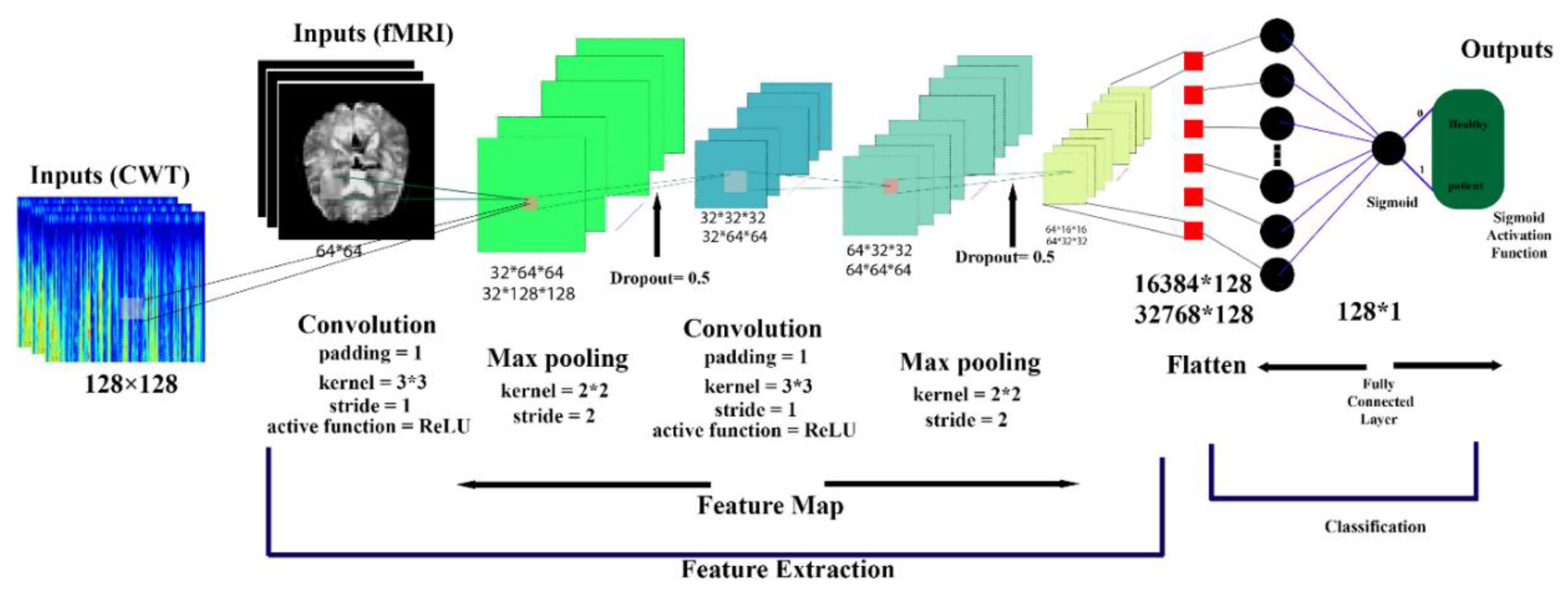
Figure 6.
VGG16-Based Architecture for rs-fMRI Brain Image Classification.
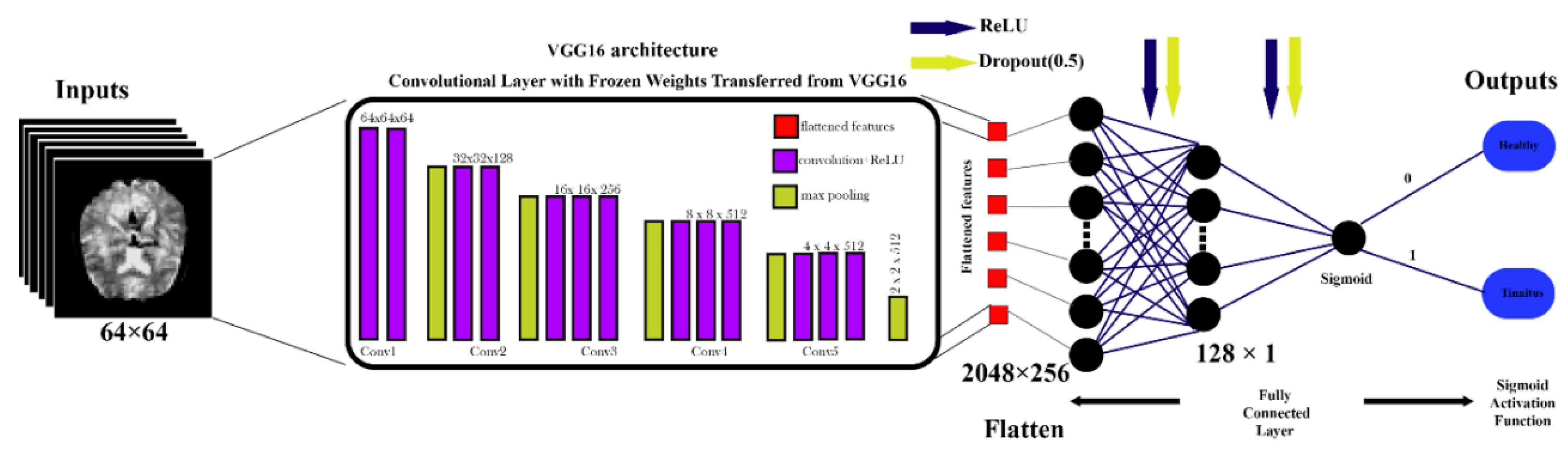
Figure 7.
ResNet-Based Architecture for rs-fMRI Brain Image Classification.
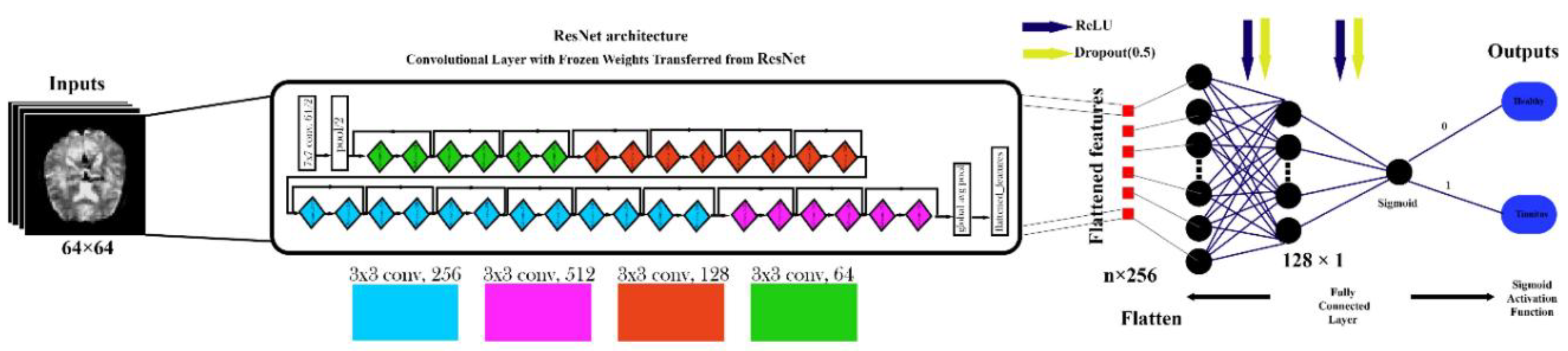
Figure 8.
Proposed Framework for EEG Signal and rs-fMRI Image Processing with Multi-Model Classification.
Figure 8.
Proposed Framework for EEG Signal and rs-fMRI Image Processing with Multi-Model Classification.
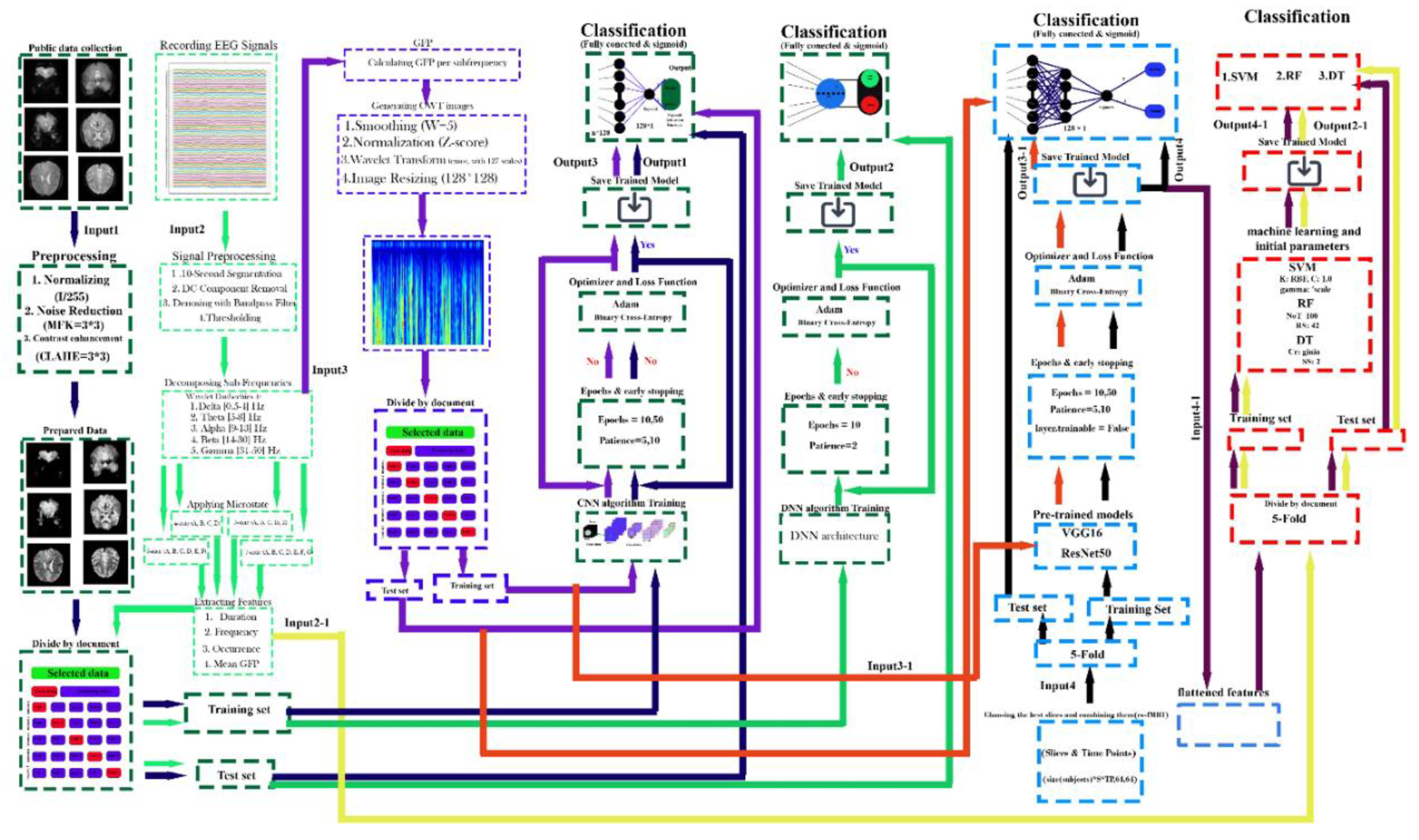
Figure 10.
Comprehensive CNN Performance Analysis for rs-fMRI Data Classification Across 32 Axial Slices. (a) CNN classification performance metrics (Precision, Accuracy, Recall, F1 Score, and ROC AUC) across 32 axial rs-fMRI slices, evaluated using subject-level 5-fold cross-validation. Each subject contributes 400 timepoint images per slice. The x-axis represents axial slice indices, sorted in ascending order by accuracy. Shaded areas indicate standard deviation across folds. (b) Mean confusion matrices (across 5 folds) for each axial slice, showing classification outcomes between healthy controls and tinnitus subjects at the timepoint level.
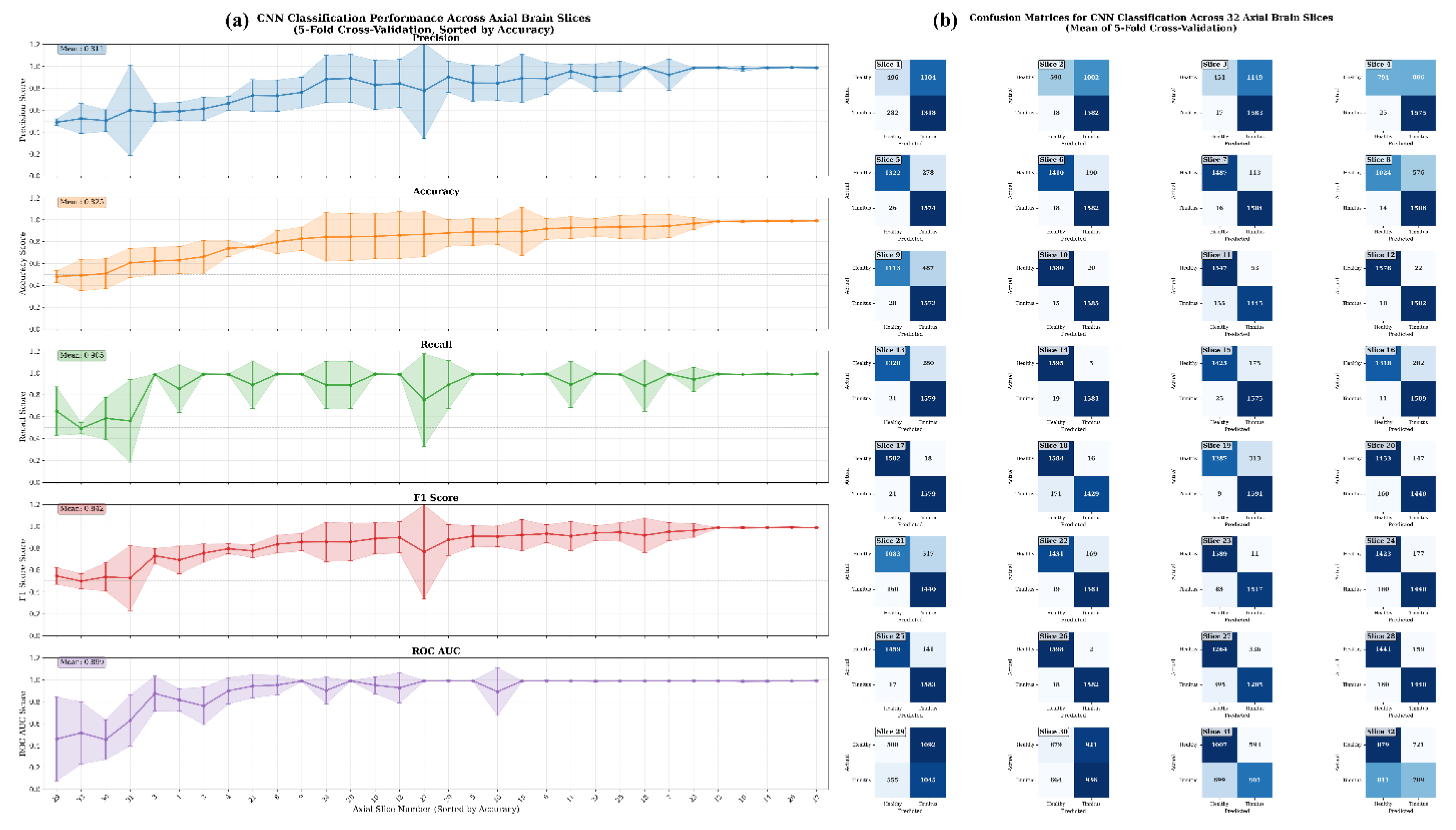
Figure 11.
Axial fMRI Slice Comparison of Healthy and Tinnitus-Affected Brain Regions. In panel (a), the mean and standard deviation of each slice are displayed for both groups, with the x-axis representing the slice order and the y-axis showing the mean and standard deviation of pixel intensity differences in the final image. Panel (b) presents the maximum pixel intensity differences at different time points for healthy (odd-numbered columns from the left) and tinnitus (even-numbered columns from the left) groups. A customized color map highlights these differences, with red indicating higher intensity changes. The results reveal distinct patterns of neural activity and potentially affected regions in tinnitus patients. The color bar represents the pixel intensity difference scale.
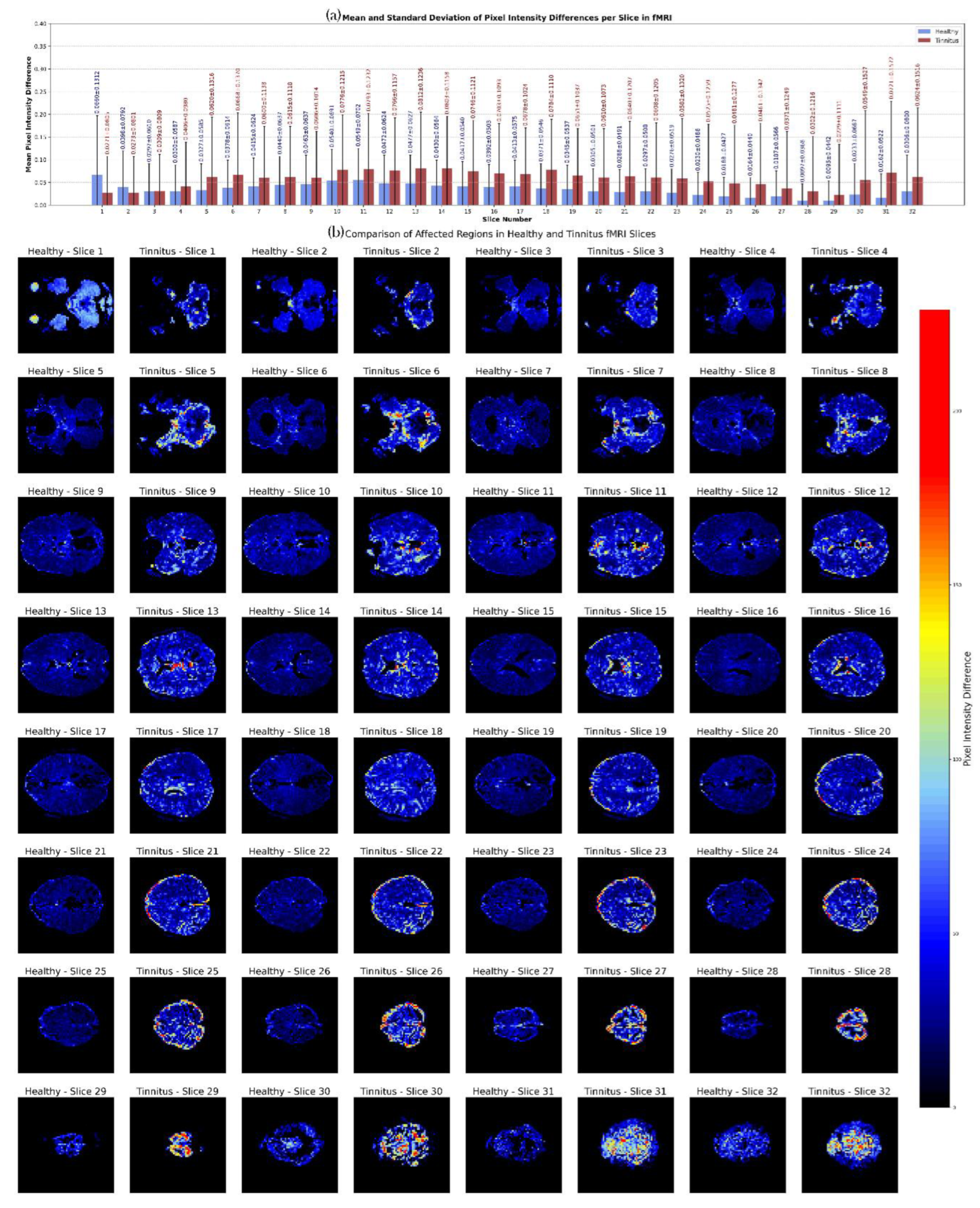
Figure 12.
Performance Comparison of Pre-trained and Hybrid Models for fMRI-based Tinnitus Classification. Data represent mean ± standard deviation from 5-fold cross-validation on test data. The red dashed line indicates the 95% clinical relevance threshold. Hybrid models combine pre-trained CNN feature extraction with traditional machine learning classifiers (Decision Tree, Random Forest, Support Vector Machine) for automated tinnitus detection.
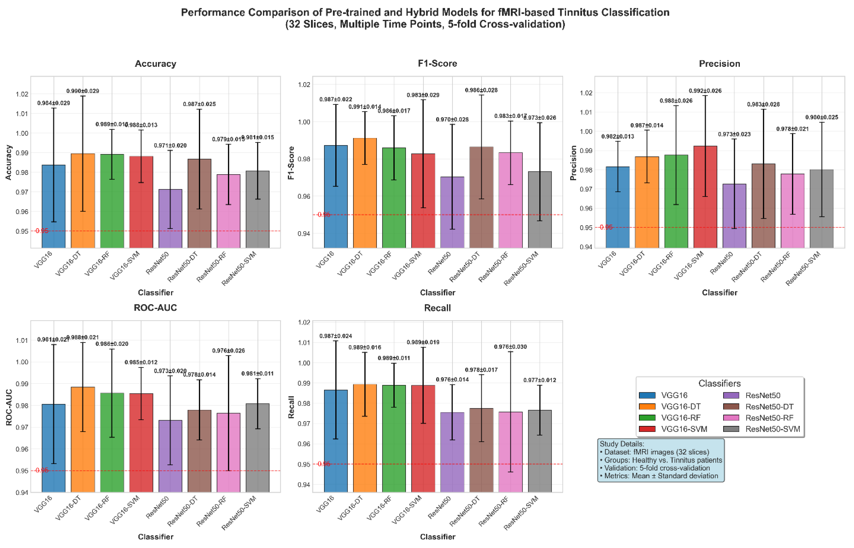
Figure 13.
Comprehensive Statistical and Visual Comparison of Microstate Features Across Configurations and Frequency Bands in Healthy vs. Tinnitus Groups: Statistical Power (a) Significance Patterns (b) Microstate Feature Comparison (c). Subfigure (a) illustrates the statistical power across microstate configurations and frequency bands, highlighting the varying effect strengths. Subfigure (b) summarizes significance rates across configurations, feature types, and frequency bands, along with the distribution of effect sizes. Subfigure (c) compares five key microstate features (duration, coverage, occurrence, and mean GFP) between groups across all configurations and frequency bands. Statistically significant group differences (p < 0.05) are marked with red asterisks.
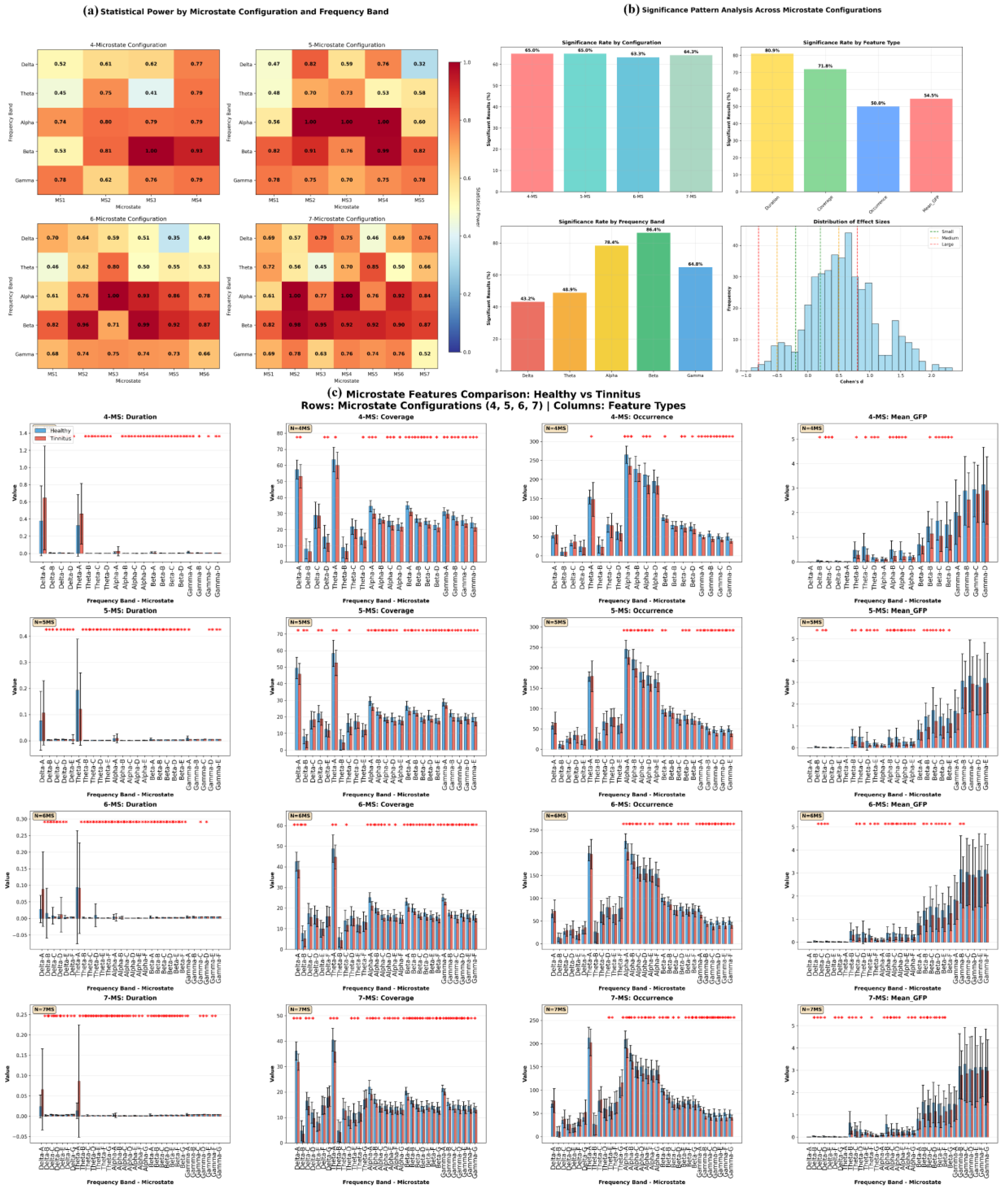
Figure 14.
Performance Evaluation of Machine Learning Classifiers for EEG-based Tinnitus Classification Using Comprehensive Microstate Features. Panel (a) presents bar charts comparing five key performance metrics across the four algorithms with error bars indicating variability, alongside a numerical summary table. Panel (b) displays ROC curves that demonstrate the discrimination capability of each classifier against the diagonal reference line. Panel (c) shows 2×2 confusion matrices for each classifier, presenting average classification results with both absolute counts and percentage distributions.
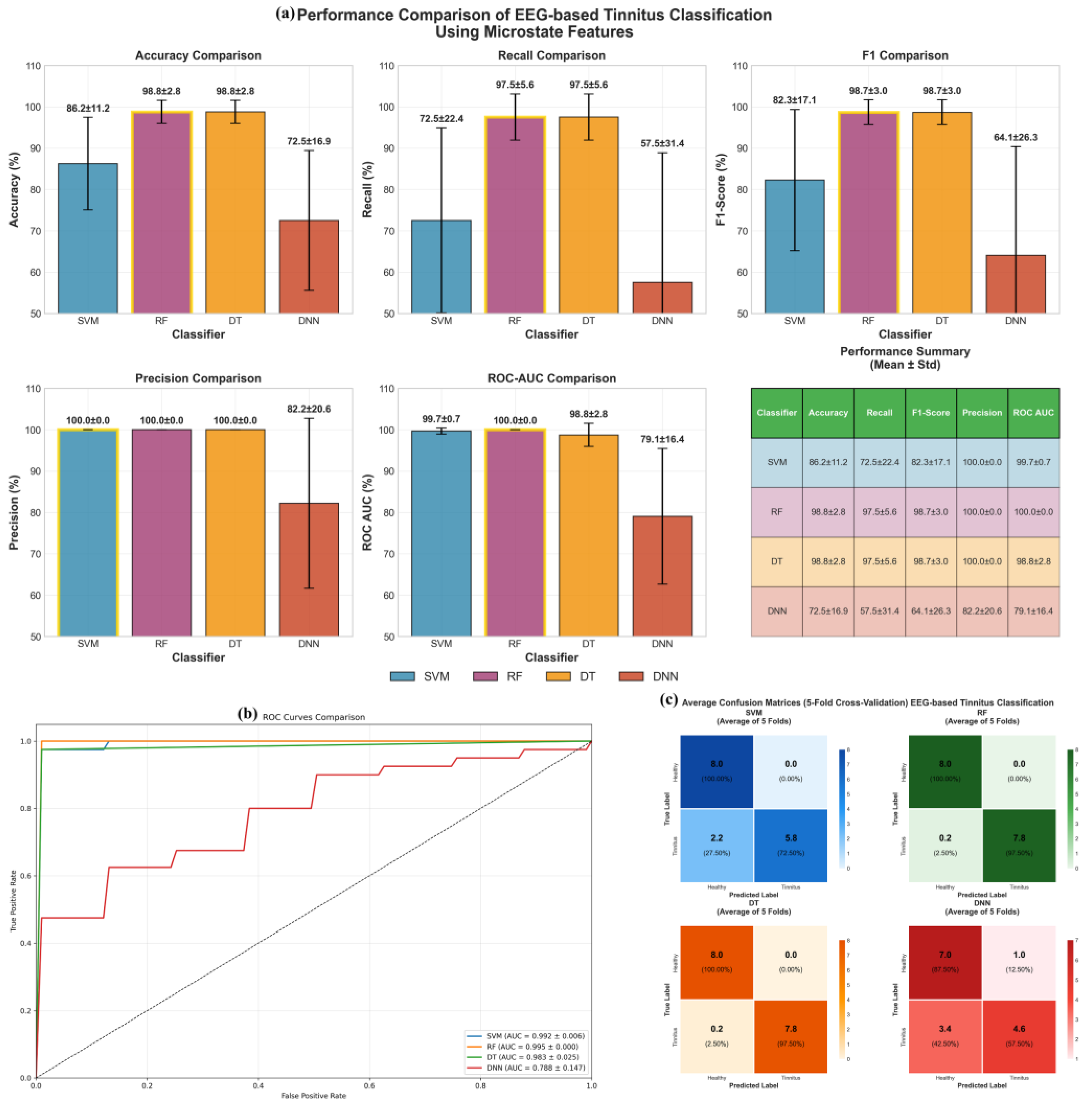
Figure 15.
EEG-Based Classification Performance Across Microstate Configurations and Frequency Bands.
Figure 15.
EEG-Based Classification Performance Across Microstate Configurations and Frequency Bands.
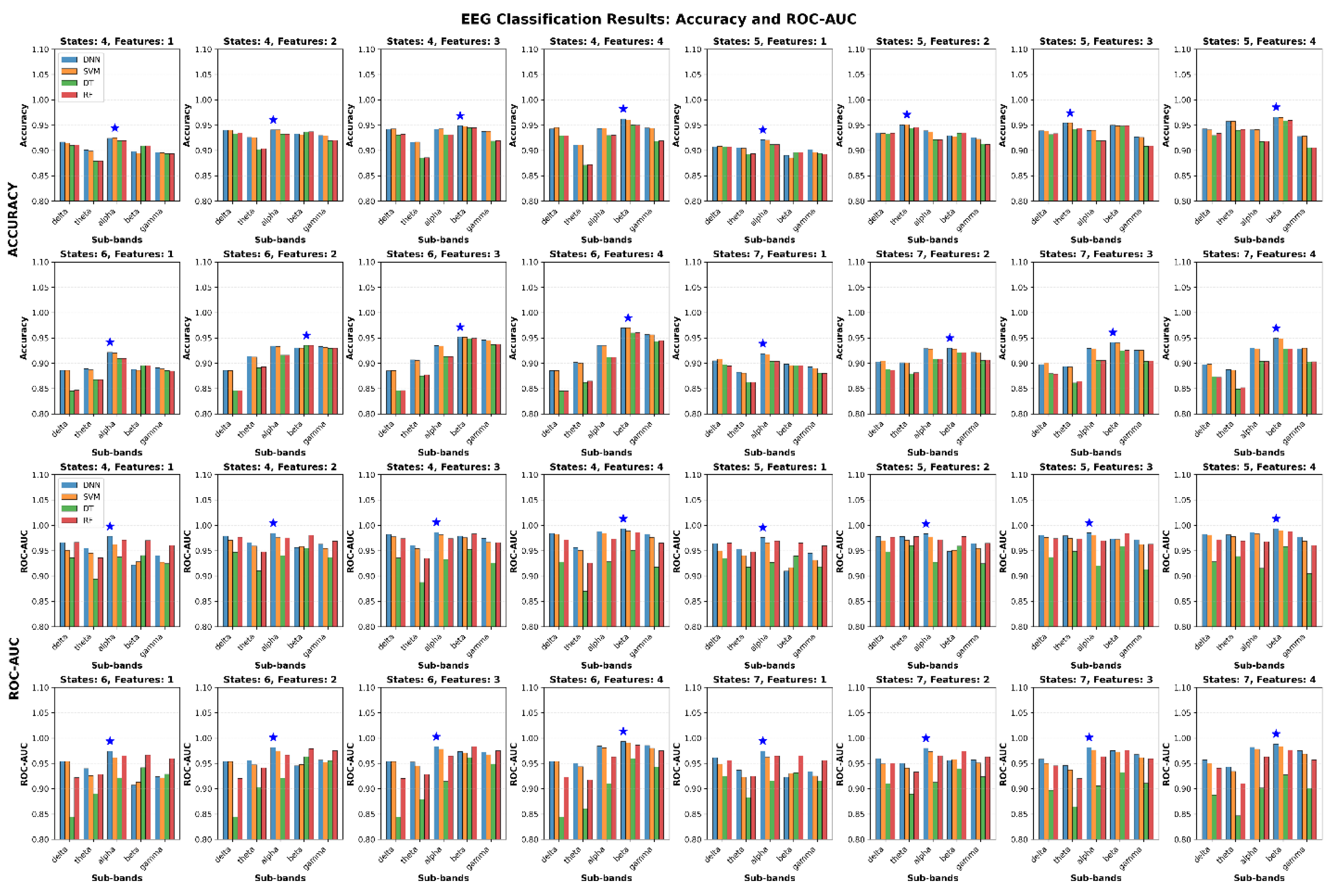
Table 1.
Clinical and Audiological Characteristics of Primary Tinnitus Cohort.
| ID | Sex | Age | Tinnitus Phenotype | Frequency (Hz) | Loudness (dB SL) | Hearing Threshold (dB HL) | Audiometric Index | Anxiety Score | Depression Score | Severity Rating | Laterality |
|---|---|---|---|---|---|---|---|---|---|---|---|
| T01 | F | 52 | Tonal | 6100 | 32 | 12 | 17 | 2 | 2 | Mild | Left |
| T02 | M | 35 | Tonal | 1550 | 14 | 7 | 9 | 2 | 1 | Minimal | Right |
| T03 | M | 61 | Tonal | 10100 | 52 | 10 | 19 | 1 | 2 | Minimal | Left |
| T04 | F | 45 | Complex | 8100 | 48 | 23 | 27 | 2 | 2 | Moderate | Left |
| T05 | F | 29 | Tonal | 7900 | 16 | 17 | 22 | 1 | 1 | Minimal | Right |
| T06 | F | 68 | Tonal | 11300 | 88 | 9 | 13 | 2 | 2 | Severe | Left |
| T07 | M | 42 | Tonal | 1950 | 37 | 19 | 15 | 1 | 1 | Minimal | Right |
| T08 | F | 38 | Complex | 7450 | 26 | 19 | 23 | 2 | 2 | Minimal | Left |
| T09 | F | 31 | Tonal | 5900 | 11 | 14 | 15 | 1 | 1 | Severe | Right |
| T10 | F | 56 | Tonal | 9100 | 42 | 18 | 25 | 2 | 2 | Severe | Left |
| T11 | M | 49 | Tonal | 4050 | 12 | 19 | 20 | 3 | 2 | Minimal | Right |
| T12 | M | 33 | Complex | 2950 | 24 | 14 | 13 | 1 | 1 | Absent | Left |
| T13 | F | 47 | Tonal | 4950 | 46 | 21 | 24 | 2 | 1 | Minimal | Right |
| T14 | M | 36 | Tonal | 2525 | 32 | 13 | 11 | 2 | 1 | Minimal | Right |
| T15 | F | 54 | Complex | 6950 | 49 | 15 | 19 | 1 | 1 | Severe | Left |
| T16 | F | 41 | Tonal | 10050 | 57 | 22 | 31 | 2 | 2 | Moderate | Right |
| T17 | M | 28 | Tonal | 2050 | 21 | 20 | 22 | 1 | 1 | Minimal | Left |
| T18 | F | 58 | Tonal | 6050 | 36 | 17 | 21 | 2 | 1 | Severe | Right |
| T19 | M | 39 | Tonal | 4050 | 16 | 13 | 14 | 1 | 1 | Minimal | Left |
| T20 | F | 44 | Complex | 8050 | 22 | 42 | 47 | 2 | 2 | Severe | Right |
| T21 | M | 32 | Tonal | 3200 | 28 | 15 | 18 | 2 | 1 | Mild | Left |
| T22 | F | 48 | Complex | 9200 | 35 | 18 | 24 | 1 | 2 | Moderate | Right |
| T23 | M | 26 | Tonal | 4800 | 19 | 11 | 14 | 1 | 1 | Minimal | Left |
| T24 | F | 53 | Tonal | 7200 | 44 | 21 | 26 | 2 | 2 | Severe | Right |
| T25 | M | 37 | Complex | 5400 | 31 | 16 | 20 | 2 | 1 | Mild | Left |
| T26 | F | 46 | Tonal | 8800 | 39 | 19 | 23 | 1 | 2 | Moderate | Right |
| T27 | M | 30 | Tonal | 2800 | 22 | 13 | 16 | 1 | 1 | Minimal | Left |
| T28 | F | 59 | Complex | 6600 | 47 | 24 | 29 | 2 | 2 | Severe | Right |
| T29 | M | 43 | Tonal | 3600 | 26 | 17 | 21 | 2 | 1 | Mild | Left |
| T30 | F | 34 | Tonal | 9600 | 33 | 14 | 18 | 1 | 1 | Moderate | Right |
| T31 | M | 51 | Complex | 4200 | 41 | 20 | 25 | 2 | 2 | Severe | Left |
| T32 | F | 40 | Tonal | 7800 | 29 | 16 | 22 | 1 | 1 | Mild | Right |
| T33 | M | 27 | Tonal | 5200 | 24 | 12 | 15 | 1 | 1 | Minimal | Left |
| T34 | F | 55 | Complex | 8400 | 45 | 22 | 27 | 2 | 2 | Severe | Right |
| T35 | M | 38 | Tonal | 3800 | 30 | 18 | 23 | 2 | 1 | Moderate | Left |
| T36 | F | 47 | Tonal | 6400 | 37 | 20 | 25 | 1 | 2 | Moderate | Right |
| T37 | M | 24 | Complex | 4600 | 25 | 14 | 17 | 1 | 1 | Minimal | Left |
| T38 | F | 60 | Tonal | 7600 | 43 | 25 | 30 | 2 | 2 | Severe | Right |
| T39 | M | 45 | Tonal | 5000 | 34 | 19 | 24 | 2 | 1 | Moderate | Left |
| T40 | F | 41 | Complex | 9000 | 40 | 17 | 21 | 1 | 2 | Moderate | Right |
Note: Tinnitus phenotypes classified as "Tonal" (narrow-band, pure-tone characteristics) or "Complex" (broadband, multi-component features). Loudness expressed in dB sensation level (SL) above individual hearing thresholds. Severity ratings based on standardized clinical assessment scales.
Table 2.
Demographic and Clinical Characteristics of fMRI Tinnitus Participants.
| Subject | Age (years) | Laterality | Duration (years) | THI Score | Trauma Etiology | Right Ear Loss | Left Ear Loss |
| P1 | 55 | Bilateral | 11 | 7 | Occupational | 2-8 kHz | 0.25, 8 kHz |
| P2 | 44 | Bilateral | 26 | 9 | Military | - | 0.5 kHz |
| P3 | 39 | Bilateral | 14 | 24 | Military | 4-8 kHz | 4-8 kHz |
| P4 | 60 | Bilateral | 26 | 23 | Military | 4-8 kHz | 4-8 kHz |
| P5 | 29 | Bilateral | 11 | 9 | Musical | - | - |
| P6 | 41 | Bilateral | 3 | 15 | Military | 0.5-1, 8 kHz | 8 kHz |
| P7 | 42 | Bilateral | 15 | 31 | Military | 8 kHz | 8 kHz |
| P8 | 43 | Bilateral | 17 | 23 | Combined | 0.25-4 kHz | 2-8 kHz |
| P9 | 50 | Left | 11 | 45 | Military | 0.25-8 kHz | 0.25-8 kHz |
| P10 | 41 | Right | 17 | 17 | Military | - | - |
| P11 | 27 | Left | 2 | 13 | Military | - | 4-8 kHz |
| P12 | 59 | Bilateral | 18 | 11 | Military | 0.25-0.5 kHz | 0.25-8 kHz |
| P13 | 23 | Bilateral | 2 | 25 | Musical | - | - |
| P14 | 26 | Bilateral | 17 | 5 | Musical | - | - |
| P15 | 41 | Right | 3 | 13 | Musical | 4-8 kHz | 0.5, 8 kHz |
| P16 | 50 | Right | 0.5 | 13 | Military | 4-8 kHz | 8 kHz |
| P17 | 58 | Bilateral | 11 | 7 | Occupational | 4-8 kHz | 4-8 kHz |
| P18 | 50 | Left | 11 | 15 | Musical | - | - |
| P19 | 34 | Bilateral | 14 | 5 | Military | - | 0.25-0.5 kHz |
THI: Tinnitus Handicap Inventory. Hearing loss frequencies indicate ranges with elevated thresholds (>20 dB HL).
Table 3.
rs-fMRI Dataset Structure and Organization.
| Parameter | Value | Description |
|---|---|---|
| Total Subjects | 38 | 19 tinnitus patients + 19 healthy controls |
| Tinnitus Subjects | 19 | Chronic tinnitus from acoustic trauma |
| Control Subjects | 19 | Age-matched healthy controls |
| Axial Slices per Subject | 32 | Whole-brain coverage with 3.5 mm thickness |
| Time Points per Subject | 400 | Acquired over 13 minutes 20 seconds |
| Total Images per Subject | 12,800 | 32 slices × 400 time points |
| Total Dataset Images | 486,400 | 38 subjects × 12,800 images |
| Spatial Resolution | 3 × 3 mm² | In-plane resolution |
| Temporal Resolution (TR) | 2000 ms | Repetition time |
| Acquisition Duration | 13:20 min | Total scanning time per subject |
Table 4.
Summary of Preprocessing Steps.
| Modality | Preprocessing Step | Description | Equation |
| EEG | Data Segmentation and Filtering [24] | Segmented into 10-second epochs (1200 samples per epoch) and filtered using a 3rd-order Butterworth bandpass filter (0.5–50 Hz). | |
| EEG | Normalization and DC Correction [25] | Normalized to = mean (), std ()= 1, with DC offset correction by subtracting the mean from each segment. | |
| EEG | Outlier Removal | Segments with voltage outside -150 to 150 µV were excluded to remove artifacts like eye blinks and muscle activity. | --- |
| EEG | Frequency Decomposition [24] | Decomposition of the EEG signal into Delta (0.5-4 Hz), Theta (5-8 Hz), Alpha (9-14 Hz), Beta (15-30 Hz), and Gamma (31-50 Hz) bands using the wavelet transform with the Daubechies 4 (Db4) wavelet. | |
| rs-fMRI | Normalization | Scaled pixel intensity values to [0, 1] by dividing by 255. | = |
| rs-fMRI | Noise Reduction [26] | Applied a median filter (kernel size 3×3) to reduce noise while preserving edges. | |
| rs-fMRI | Contrast Enhancement [27] | Enhanced contrast using CLAHE with a 3×3 kernel to improve local contrast while preventing noise amplification. |
Table 5.
Feature Extraction and Dataset Specifications.
| Parameter | Specification | Details |
|---|---|---|
| Participants | 80 | 40 tinnitus patients, 40 healthy controls |
| Recording Duration | 5 minutes | Resting-state EEG |
| Window Segmentation | 10-second non-overlapping | 300 windows per participant |
| Total Windows | 24,000 | 300 windows × 80 participants |
| Frequency Sub-bands | 5 bands | Delta (1–4 Hz), Theta (4–8 Hz), Alpha (8–13 Hz), Beta (13–30 Hz), Gamma (30–45 Hz) |
| Microstate Configurations | 4 models | 4-state (A–D), 5-state (A–E), 6-state (A–F), 7-state (A–G) |
| Microstate Parameters | 4 features per state | Duration, Coverage, Occurrence, Mean GFP |
| Features per Configuration | Varies by model | 4-state: 80, 5-state: 100, 6-state: 120, 7-state: 140 |
| Total Features per Window | 440 | Combined from all configurations |
| Final Dataset Dimensions | 24,000 × 440 | Windows × Features matrix |
| Classification Samples | 24,000 | 12,000 tinnitus, 12,000 control windows |
Table 6.
Feature Extraction Methods and Formulas for Microstate Analysis in EEG Data.
| Feature | Description | Formula | Parameters Explanation |
| Duration [35] | The average time a microstate remains stable without switching. | | Duration of microstate i, N: Total number of microstates in the signal. |
| Occurrence [36] | The number of times a specific microstate occurs per second. | N: Total number of occurrences of the microstate, T: Total duration of the EEG signal. | |
| Coverage [36] | Indicates the proportion of the total analysis time occupied by each microstate class. | : Duration of microstate i, T: Total duration of the EEG signal. | |
| GFP (Global Field Power) [37] | The spatial variance of the EEG signal at a specific time point. | :Voltage at electrode iii at time t, : Mean voltage at time t, n: Number of electrodes. |
Table 7.
Pipeline for generating CWT images from GFP signals extracted from EEG data.
| Step | Description |
|---|---|
| GFP Extraction | Computed from each of the 64 channels and 5 frequency bands |
| Smoothing | Moving average filter (window size = 5) |
| Normalization | Z-score normalization |
| Wavelet Transform | Continuous wavelet transform using cmor, with 127 scales |
| Image Resizing | Resized to 128×128 pixels and normalized for CNN input |
Table 9.
Top 15 EEG Microstate Findings: Healthy vs Tinnitus.
| Rank | Cluster Solution | Frequency Band | Microstate | Feature | Healthy Mean | Tinnitus Mean | Cohen's d | P-value | Statistical Power |
|---|---|---|---|---|---|---|---|---|---|
| 1 | 7-state | Gamma | B | Occurrence (events/epoch) | 56.56 | 43.81 | 2.11 | 1.58×10⁻¹⁴ | 1.000 |
| 2 | 4-state | Alpha | A | Coverage (%) | 34.62% | 29.95% | 1.48 | 3.80×10⁻⁹ | 1.000 |
| 3 | 5-state | Alpha | B | Duration (ms) | 1.23 ms | 1.11 ms | 1.89 | 1.25×10⁻¹² | 1.000 |
| 4 | 6-state | Beta | A | Coverage (%) | 23.09% | 20.28% | 1.58 | 6.06×10⁻¹⁰ | 1.000 |
| 5 | 4-state | Beta | A | Coverage (%) | 35.14% | 31.06% | 1.81 | 6.59×10⁻¹² | 1.000 |
| 6 | 7-state | Alpha | B | Duration (ms) | 1.12 ms | 0.99 ms | 2.20 | 5.40×10⁻¹⁴ | 1.000 |
| 7 | 6-state | Gamma | A | Occurrence (events/epoch) | 76.79 | 62.95 | 2.34 | 1.77×10⁻¹⁶ | 1.000 |
| 8 | 4-state | Alpha | A | Occurrence (events/epoch) | 264.81 | 234.90 | 1.39 | 2.32×10⁻⁸ | 1.000 |
| 9 | 5-state | Gamma | A | Occurrence (events/epoch) | 68.17 | 57.52 | 1.70 | 5.79×10⁻¹¹ | 1.000 |
| 10 | 7-state | Gamma | A | Occurrence (events/epoch) | 69.65 | 60.32 | 1.75 | 1.89×10⁻¹¹ | 1.000 |
| 11 | 4-state | Theta | D | Mean GFP (μV) | 0.191 | 0.113 | 1.08 | 9.67×10⁻⁶ | 1.000 |
| 12 | 6-state | Alpha | A | Coverage (%) | 25.16% | 21.09% | 1.86 | 2.11×10⁻¹² | 1.000 |
| 13 | 5-state | Beta | D | Duration (ms) | 3.31 ms | 2.93 ms | 1.54 | 1.28×10⁻⁹ | 1.000 |
| 14 | 7-state | Beta | D | Duration (ms) | 2.70 ms | 2.34 ms | 1.72 | 3.78×10⁻¹¹ | 1.000 |
| 15 | 6-state | Gamma | B | Occurrence (events/epoch) | 51.82 | 43.51 | 1.40 | 1.89×10⁻⁸ | 1.000 |
Table 10.
Pairwise ROC-AUC Comparisons Using the DeLong Test Between Classifiers.
| Classifier 1 | Classifier 2 | AUC₁ | AUC₂ | Z-statistic | P-value | Significant |
|---|---|---|---|---|---|---|
| SVM | RF | 0.9969 | 1.0000 | -0.0828 | 0.9340 | No |
| SVM | DT | 0.9969 | 0.9875 | 0.2518 | 0.8012 | No |
| SVM | DNN | 0.9969 | 0.8125 | 3.1363 | 0.0017 | Yes |
| RF | DT | 1.0000 | 0.9875 | 0.3601 | 0.7188 | No |
| RF | DNN | 1.0000 | 0.8125 | 3.1354 | 0.0017 | Yes |
| DT | DNN | 0.9875 | 0.8125 | 2.9327 | 0.0034 | Yes |
Table 11.
Best Performance per Classifier (Accuracy & ROC-AUC).
| Classifier | Sub-band | States | Features | Best Accuracy | Best ROC-AUC |
| DNN | Beta | 6 | 4 | 0.9696 | 0.9932 |
| SVM | Beta | 6 | 4 | 0.9698 | 0.9905 |
| DT | Beta | 6 | 4 | 0.9600 | 0.9622 |
| RF | Beta | 6 | 4 | 0.9602 | 0.9874 |
Table 12.
Sub-band Performance Analysis (Mean Performance Across All Configurations).
| Sub-band | Mean Accuracy ± SD | Mean ROC-AUC ± SD |
| Delta | 0.9063 ± 0.0234 | 0.9447 ± 0.0287 |
| Theta | 0.9023 ± 0.0307 | 0.9353 ± 0.0349 |
| Alpha | 0.9256 ± 0.0119 | 0.9565 ± 0.0221 |
| Beta | 0.9308 ± 0.0246 | 0.9607 ± 0.0267 |
| Gamma | 0.9158 ± 0.0205 | 0.9458 ± 0.0237 |
Table 13.
Micro-state Configuration Performance (Mean Performance Across All Sub-bands and Classifiers).
Table 13.
Micro-state Configuration Performance (Mean Performance Across All Sub-bands and Classifiers).
| States | Mean Accuracy ± SD | Mean ROC-AUC ± SD |
| 4 | 0.9196 ± 0.0209 | 0.9549 ± 0.0254 |
| 5 | 0.9214 ± 0.0215 | 0.9567 ± 0.0251 |
| 6 | 0.9148 ± 0.0323 | 0.9478 ± 0.0349 |
| 7 | 0.9004 ± 0.0198 | 0.9386 ± 0.0252 |
Table 14.
Feature Combination Performance (Mean Performance Across All Sub-bands and Classifiers).
| Features | Mean Accuracy ± SD | Mean ROC-AUC ± SD |
| 1 | 0.8942 ± 0.0129 | 0.9377 ± 0.0194 |
| 2 | 0.9181 ± 0.0205 | 0.9518 ± 0.0213 |
| 3 | 0.9223 ± 0.0235 | 0.9547 ± 0.0262 |
| 4 | 0.9245 ± 0.0269 | 0.9574 ± 0.0297 |
Disclaimer/Publisher’s Note: The statements, opinions and data contained in all publications are solely those of the individual author(s) and contributor(s) and not of MDPI and/or the editor(s). MDPI and/or the editor(s) disclaim responsibility for any injury to people or property resulting from any ideas, methods, instructions or products referred to in the content. |
© 2025 by the authors. Licensee MDPI, Basel, Switzerland. This article is an open access article distributed under the terms and conditions of the Creative Commons Attribution (CC BY) license (http://creativecommons.org/licenses/by/4.0/).
Copyright: This open access article is published under a Creative Commons CC BY 4.0 license, which permit the free download, distribution, and reuse, provided that the author and preprint are cited in any reuse.


