Submitted:
20 October 2025
Posted:
21 October 2025
You are already at the latest version
Abstract
Lipid vesicles and related nanocarriers often contain two compartments, such as the inner and outer leaflets of a bilayer membrane between which amphipathic molecules can migrate. We develop a stochastic model for describing the transfer kinetics of cargo between the two compartments in an ensemble of carriers, neglecting inter-carrier exchange to focus exclusively on intra-carrier redistribution. Starting from a set of rate equations, we examine the Gaussian regime in the limit of low cargo occupation where Gaussian and Poissonian statistics overlap. We derive a Fokker–Planck equation that we solve analytically for any initial cargo distribution among the carriers. Moments of the predicted distributions and examples, including a comparison between numerical solutions of the rate equations and the analytic solutions of the Fokker–Planck equation, are presented and discussed, thereby establishing a theoretical foundation to study coupled intra- and inter-carrier transport processes in mobile nanocarrier systems.
Keywords:
stochastic model
; two-compartment
; Fokker-Planck equation
; lipid vesicle
; liposome
1. Introduction
Mobile nanocarriers are used to deliver drug molecules [1], nucleic acids [2], imaging agents [3], proteins and peptides [4], vaccines [5], and even small metabolites or signaling molecules [6,7]. They come in the form of liposomes, polymeric nanoparticles, micelles, dendrimers, lipid nanoparticles, inorganic nanoparticles, and other engineered nanostructures designed for targeted and controlled delivery [1,8]. Release of cargo from nanocarriers can occur passively through diffusion or gradual degradation of the carrier matrix, or actively in response to specific triggers such as pH, redox gradients, temperature, electric and magnetic fields, or light [9].
The passive release of cargo from a nanocarrier can occur through diffusion out of the carrier into the ambient medium or through collisions with other carriers [10]. For example, a liposome loaded with drug molecules can lose its content over time by diffusion of cargo into the aqueous environment or by random transfer of cargo into a different liposome or another target object upon collision. The acquisition of new cargo through the same two transfer modes is equally possible. Detailed modeling of these mechanisms plays an important role in understanding drug release kinetics and optimizing carrier design as well as in formulating release systems that combine passive and stimulus-responsive release [11,12,13].
Liposomes have been studied extensively as carrier vehicles for drug molecules [14], with more than a dozen formulations being currently approved by the U.S. Food and Drug Administration and the European Medicines Agency for clinical use in cancer therapy, antifungal treatment, pain management, and vaccine delivery [15,16]. The association of a drug with a liposome depends on its hydrophobicity profile. Hydrophilic drugs such as doxorubicin [17] or gemcitabine [18] localize in the aqueous core, with the bilayer acting as a barrier, whereas poorly soluble hydrophobic or amphipathic drugs such as amphotericin B [19] or temoporfin [20] embed in the lipid membrane. Even highly hydrophobic drugs show partial polarity [21], leading to asymmetric leaflet interactions, similar to cholesterol with its hydrophobic backbone buried in the bilayer and hydroxyl group anchored at the headgroup region [22]. Thus, bilayer-associated drug molecules are expected to reside predominantly in two states, being associated either with the external or internal leaflet of the membrane.
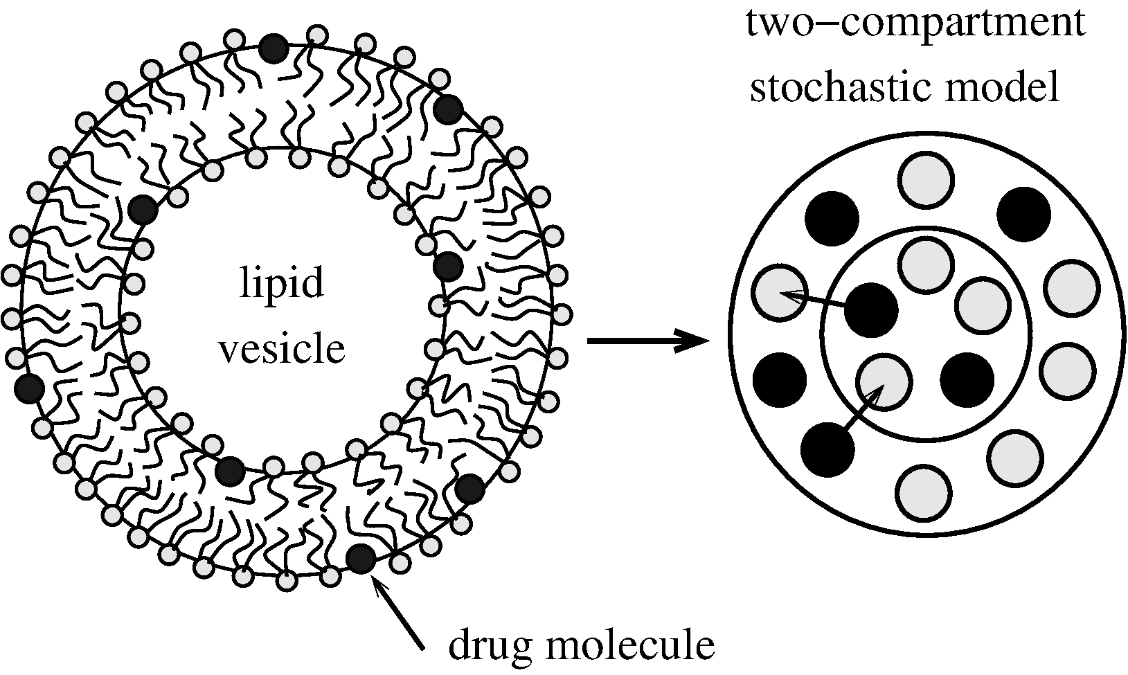
The present work aims at contributing to the development of a stochastic model for the transfer kinetics of cargo among mobile nanocarriers. The general scope is illustrated in Figure 1, which shows a schematic representation of carriers with two compartments, external and internal. Although not being displayed in Figure 1, different types of carriers may be present in a general system. Each compartment contains identical sites that are either empty or occupied by a single cargo item.
Upon the collision of two carriers, cargo residing in the external compartment of one carrier can migrate to the external compartment of another carrier. Cargo can also migrate between the two compartments of a given carrier. Hence, the migration from the internal compartment of a carrier to the internal compartment of another carrier must proceed via the two external compartments of the two carriers. Modeling the stochastic time-evolution of a suitable distribution function is a challenging task. In a preceding study [23], we have cast the problem into a set of rate equations and identified an analytic solution in the limit that each carrier contains only one single compartment, which is always filled with a sufficiently large number of cargo but is never even close to be filled completely. We have referred to that limit as the Gaussian regime at low occupation. In the present study, we consider the presence of an external and internal compartment in each carrier and allow for the transfer of cargo between the two. However, we shall not allow for the transfer of cargo between different carriers. This restriction to intra-carrier transport is a significant simplification that renders our stochastic model equivalent to first-order unimolecular reactions [24,25]. Yet, in contrast to having only one “reaction chamber”, our system consists of an ensemble of carriers and thus of one “reaction chamber” for each subpopulation of carriers with fixed total cargo content.
Studying only the internal transfer kinetics of cargo in carriers is a necessary step toward solving the composite problem of allowing for transfer both between and within carriers. Yet, even when ignoring transfer between carriers, the remaining two-compartment stochastic model is of interest because, as we show below, it allows us to express the rate equations as a Fokker-Planck equation in exactly the same limit—the Gaussian regime at low occupation—as in our preceding study [23]. We solve the Fokker-Planck equation and analyze its predictions for three specific examples, including a comparison with numerical solutions of the rate equations. Our work thus paves the way to address the full problem: a multicomponent ensemble of two-compartment carriers with both internal and collision-driven inter-carrier cargo exchange, which we plan to investigate in a future study.
2. Theoretical Model and Discussion
We describe the cargo distribution by the quantity , denoting the number of carriers that, at a given time t, contain i cargo items in their external compartment and n cargo items in their internal compartment. Each carrier possesses two compartments with identical binding sites, sites in the external and sites in the internal compartment. Every site can either be vacant or host one single cargo molecule. The total number of carriers
is conserved. Cargo can be exchanged between the external and internal compartments of each individual carrier. Hence, the first moments
of yield time-dependent total numbers of cargo in the external and internal compartment, respectively. The total number of cargo in the external and internal compartments of all carriers is conserved. As discussed in the Introduction, we do not consider transfer of cargo among different carriers, implying that does not depend on time for any fixed v with and the assumption that if or .
2.1. Rate Equations
To set up rate equations for the kinetics of intra-carrier transfer of cargo, we display in Figure 2 three carriers that illustrate the processes contributing to the rate of change of .
The population number increases for a transfer and for a transfer . Similarly, the population number decreases for a transfer and for a transfer . We associate each transfer process with a rate constant, for the transfer of cargo from the external to the internal compartment, and for the transfer of cargo from the internal to the external compartment. The rate constants and reflect passive transport properties across an energy barrier that separates the internal and external compartments. For lipid membranes, permeabilities and flip-flop rates have been studied extensively, both experimentally [26] and via computer simulations [27]. They are found to depend on a multitude of factors, including steric interactions, hydrogen bond formation, membrane composition and degree of asymmetry, the presence of cholesterol, and pH for ionizable drugs. Note that our use of a fixed, single set of rate constants, and , neglects cooperativity of transfer processes [28] and variations due to structural and chemical heterogeneities such as locally different compositions in a multi-component lipid vesicle [29,30]. In our present model, transfer events are independent from each other. The rate of change of takes the form of a chemical Master equation,
with for all and . Each term in the rate equations also includes a combinatorial factor [31],
that accounts for the random statistical occurrence of all possible cargo distributions in a transfer event from the external to the internal compartment (the left of the two equations) and from the internal to the external compartment (the right of the two equations), given the number of cargo in the external and internal compartments is i and n, respectively. Specifically, the factor accounts for the number of states for which a given cargo item can move from an occupied site in the external compartment to an empty site in the internal compartment divided by the total number of available states , multiplied by the number of available sites in the external compartment. For example, implies indicating that transfer into a completely filled internal compartment is not possible. Reasoning for the factor is analogous. Because of the presence of the factors and , Eq. 3 can also be referred to as combinatorial Master equation [32]. Based on the rate equations (Eq. 3), we can compute the first moments as defined in Eq. 2, resulting in
In the limit and or if the condition is fulfilled, the final term on the right-hand side of Eq. 5 vanishes, and the remaining differential equations for and yield the well-known exponential behavior of a first-order unimolecular reaction [33],
with the characteristic time and
Note that with and with denote the number of cargo per carrier in the external and internal compartments, respectively, at equilibrium. Hence, the total amount of cargo per carrier is . Eqs. 6 satisfy the initial conditions and with . Eqs. 6 and 7 are relevant for the present work because below in Sec. Section 2.2 we will adopt the Gaussian limit, where and .
Let us return to the rate equations (Eq. 3). In equilibrium, for , the function
takes on a binomial distribution in both i and n multiplied by a function that depends only on the sum of the two indices and ensures the normalization in Eq. 1 is satisfied. The exact form of depends on the initial distribution as will be discussed below. The probabilities p and q in Eq. 8 relate to the rate constants and , the number of sites and , and the overall number of cargo per carrier through the two equations
The equation on the left, which is a consequence of detailed balance [32], results from inserting into Eq. 3 with , and the equation on the right reflects the conservation of cargo because and . The two relationships in Eq. 9 result from taking the first moments of Eq. 8. The probabilities p and q can be calculated explicitly from Eqs. 9. The general result is somewhat cumbersome, but if both and grow large, it simply becomes
That is, Eqs. 10 become valid in the Gaussian limit, where and . Recalling Eqs. 7, we observe that and .
2.2. Continuum Representation in the Gaussian Limit at low Occupation
General analytic solutions for the rate equations in Eq. 3 are not known to us, not even in the limit of large and . To make progress, we shall consider two approximations. The first is to adopt the Gaussian limit, where both and become large, but such that p and q adopt values anywhere in the range and . It is then convenient to adopt a continuum description , where the continuous variables x and z denote the number of cargo in the external and internal compartments, respectively. That is, the discrete variables i and n in are replaced by the continuous variables x and z in .
The moments in Eqs. 1 and 2 then read , , and . The binomial distribution in Eq. 8, which is adopted in equilibrium, turns into a Gaussian,
Instead of the discrete variable in Eq. 8, we employ the corresponding continuous variable as argument of the function . It is convenient to re-express the function
in terms of a function . Eq. 12 can be viewed as the definition of the new function , given is known. The advantage of using is the simple normalization
that this function must fulfill in order to ensure Eq. 1 is satisfied.
In the Gaussian limit, Eq. 3 can be subjected to a series expansion of and in terms of and up to first order followed by setting , leading to
This equation is of first order, thus containing drift but no fluctuation terms. Solutions of Eq. 14 would describe how initial delta-peaks would move in time without widening due to fluctuations. Fluctuations would enter Eq. 14 as terms associated with second-order derivatives. Yet, these terms do not emerge correctly from extending the first-order expansion that leads from Eq. 3 to Eq. 14 to a second order expansion. To identify the fluctuation terms, we adopt a second approximation, the low occupation limit, where the number of occupied sites in the external and internal compartment is always much smaller than the number of available sites. The corresponding conditions and imply and . Note that and both remain finite. Mathematically, the small occupation limit uses the Gaussian distribution to approximate a Poisson distribution for large mean value [34]. The equilibrium distribution specified in Eqs. 11 and 12 then reads
with the function satisfying the normalization in Eq. 13. In the low occupation limit, the terms and in Eq. 14 are negligibly small, and it becomes straightforward to identify the missing second-order fluctuation term by comparing the stationary solutions of Eq. 14 with Eq. 15. The resulting equation
is a Fokker-Planck equation [32] for the distribution , with . We reiterate that the drift term, which is associated with the first derivatives, follows from Eq. 14 in the limit of large and and employs the definitions of and in Eq. 7. The fluctuation term, which accounts for the second order derivatives in Eq. 16, ensures the equilibrium distribution of Eq. 16 is given by Eq. 15.
2.3. Solution of the Fokker-Planck Equation
In order to solve Eq. 16 we introduce the new independent variables and . This is motivated by the conservation of the total number of cargo, v, in each carrier population as u varies. The function then satisfies the equation
Because we adopted the Gaussian limit, the new variables u and v vary from to ∞. Also, note that . Hence, solutions of Eq. 17 must conserve the number of carriers and the total number of cargo . Let us specify an initial distribution . Solutions of Eq. 17,
can be constructed using the Green’s function,
with
The Green’s function , defined through Eqs. 19 and 20, satisfies the Fokker-Planck equation (Eq. 17) and is normalized such that . It initially produces a delta-peak at position — that is, the Green’s function satisfies the initial condition , where denotes the Dirac delta function. Hence, Eq. 18 reproduces the initial distribution in the limit . In the opposite limit, at , the Green’s function
is independent of , and Eq. 18 thus yields
The normalization together with Eq. 13 implies is conserved. The integral in Eq. 22 is thus . Using this, together with Eq. 21 and the definitions and , renders Eq. 22 identical to Eq. 15, thus reproducing the correct equilibrium distribution.
It is also interesting to calculate moments of our solution in Eq. 18. The first moment with respect to v yields
demonstrating that our solution indeed conserves M. It can analogously be concluded that higher moments in v are all conserved, implying that distribution functions can change with time in the direction but not in the direction. The first moment with respect to u results in
thus reproducing and according to Eq. 6. To transition from the first to the second line of Eq 24, we have made use of (see Eq. 7), , , , and (see Eq. 20). Calculation of the second moment with respect to u gives rise to
where we have used , and where we have defined the initial value (at ) of the second moment,
with analogous definitions for and . Note is conserved, as discussed above. Eq. 25 demonstrates how the second moment with respect to u propagates in time from the initial to the final value,
which depends on . That is, if two initial distributions differ in their second moment , then their equilibrium distributions will also be different, given that . Based on in Eq. 25 and in Eq. 24, the calculation of the variance is straightforward. As pointed out, the corresponding variance in the v-direction, is independent of time.
2.4. Three Specific Examples
The following three examples illustrate simple cases for the calculation of from a given initial distribution , rate constants and , and overall cargo-to-carrier ratio .
2.4.1. First Example
Assume all N carriers contain exactly the same number of cargo, , in each carrier, and all of that is initially contained exclusively in the external compartment, and . Our assumptions amount to the initial distribution function . The general solution in Eq. 18 then reads . Because of the presence of the delta-peak , it is convenient and sufficient to focus on
with specified in Eq. 20. Eq. 28 describes how the distribution shifts from the initial delta-peak at and to a Gaussian at and . Expressed in terms of x and z, this shift occurs from the initial and to the final and . Calculation of relevant moments gives rise to , , , and . The latter reflects the time evolution of the Green’s function, consistent with our initial distribution consisting of a delta-peak.
2.4.2. Second Example
We assume an initially Gaussian distribution
where we recall from Eq. 6 the initial numbers of cargo per carrier, and in the two compartments, with being the combined number. Using , we can calculate the function
Inserting into Eq. 15 yields the equilibrium distribution
Calculating the full kinetic behavior from according to Eqs. 17-20 leads to somewhat cumbersome expressions but can, of course, be carried out numerically. Here, we focus on the specific case and , where the initial distribution of the cargo in the two compartments is opposite of the preferred one. This leads to the simple analytic result,
where the limiting values for and ,
agree with Eq. 29 and 31. The left diagram of Figure 3 shows a contour plot of according to Eq. 32 for at the five different times specified in the legend.
The dashed line displays the path
along which the maximum of the Gaussian distribution moves over time until reaching equilibrium. Eqs. 34 are identical to Eqs. 6, with the specific choices of our current example. Because of , this path is linear, with a slope of the dashed line in Figure 3. The probability distributions along all lines of slope correspond to a total number of cargo . That is, only but not changes along a line of slope . Note also in Eq. 34 occurs after a time . Hence, for the green curves in Figure 3 the cargo is distributed equally among external and internal compartment, . The sequence of the five selected times , , , , and ∞, in Figure 3 corresponds to , , , , and .
Moments for our specific example can be calculated using the general formalism in Eqs. 23-25 or, equivalently, directly from the solution in Eq. 32, yielding for the variances
As pointed out above, averaging over v yields time-independent results. The corresponding variance in the u-direction is for and , but adopts a minimum at . Hence, the variances for the distributions at (purple) and (red) in the left diagram of Figure 3 are the same in the -direction and in the -direction. At all intermediate times, the variance in the -direction is smaller than that in the -direction, with the largest difference for (shown in green).
The right diagram in Figure 3 shows cross-sections of along the direction of the dashed line in the left diagram, where is fixed. Curves are displayed for the same set of times as in the left diagram, with the same color code. The solid lines correspond to in Eq. 32. The open circles show numerical solutions of the corresponding discrete rate equations, Eq. 3, with and , , , and an initial distribution , where and . Optimal agreement is expected in the limit and . Our calculations were performed for , which also leads to excellent matching. The comparison in the right diagram of Figure 3 of corresponding numerical solutions for the discrete rate equations in Eq. 3 and analytic solutions of the Fokker-Planck equation in Eq. 16 reinforces the equivalence of the two approaches.
2.4.3. Third Example
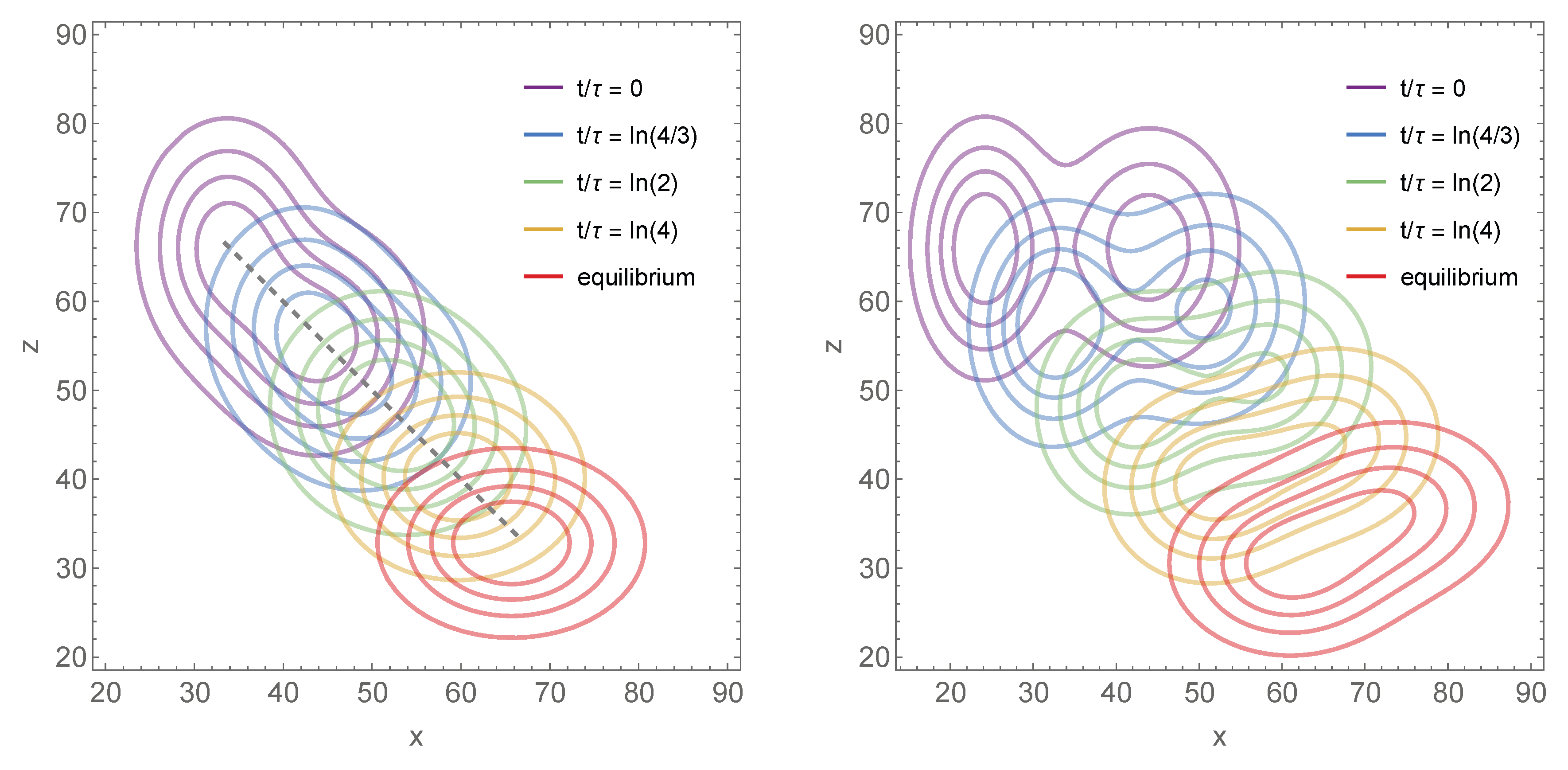
Our final example illustrates the addition of another Gaussian distribution to the initial distribution . That is, we replace the single Gaussian distribution in Eq. 29 by the sum of two Gaussians,
The two diagrams of Figure 4 show for two specific choices for the parameters , , , , and . The rate constants and as well as are the same as in Figure 3.
In the left diagram, the two Gaussians of Figure 3 for and are added, with giving each contribution the same weight. That is, , , , and were specified. Contour lines of the resulting initial distribution are displayed in purple. The cumulative probabilities as well as and are the same in Figure 3 and the left diagram of Figure 4. Hence, the equilibrium distributions (with contour lines shown in red) are the same.
In the right diagram, we separate the two Gaussians along the x-axis by choosing , , as well as . The purple contour lines represent . Here, the initial distribution evolves toward a different final distribution (with contour lines shown in red) because for the right diagram of Figure 4 is different from for Figure 3 and the left diagram of Figure 4.
3. Conclusions
This work presents a stochastic model for the kinetics of cargo transfer among two compartments that each contain identical sites but different affinities. We show that rate equations give rise to a Fokker-Planck equation in the continuum and low occupation limits, where the Gaussian and Poisson regimes of a binomial distribution overlap. That implies a large number of cargo must be present yet without ever approaching full occupation of either compartment. Analytic solutions of the Fokker-Planck equation are presented, based on identifying a Green’s function, and discussed in terms of moments and three specific examples. We emphasize that our model represents a step towards rationalizing the kinetics of collision-dominated cargo transfer among mobile two-compartment nanocarriers such as drug molecules associated with the inner or outer leaflets of lipid vesicles. While a preceding study has focused on the inter-carrier transfer of cargo [23], the present one addresses the intra-carrier transport. Future work will combine the two models into one comprehensive approach.
Author Contributions
Conceptualization, S.M.; methodology, G.V.B. and S.M.; software, G.V.B.; validation, F.H. and G.V.B.; investigation, F.H. and S.M.; writing—original draft preparation, F.H.; writing—review and editing, S.M. and G.V.B.
Funding
G. V. B. thanks Fondecyt (grant no. 11240064) for the financial support.
Conflicts of Interest
The authors declare no conflict of interest. The funders had no role in the design of the study; in the collection, analyses, or interpretation of data; in the writing of the manuscript, or in the decision to publish the results.
References
- Chamundeeswari, M.; Jeslin, J.; Verma, M.L. Nanocarriers for drug delivery applications. Environ. Chem. Lett. 2019, 17, 849–865. [Google Scholar] [CrossRef]
- Ramasamy, T.; Munusamy, S.; Ruttala, H.B.; Kim, J.O. Smart nanocarriers for the delivery of nucleic acid-based therapeutics: a comprehensive review. Biotechnol. J. 2021, 16, 1900408. [Google Scholar] [CrossRef]
- Silindir-Gunay, M.; Sarcan, E.T.; Ozer, A.Y. Near-infrared imaging of diseases: A nanocarrier approach. Drug Dev. Res. 2019, 80, 521–534. [Google Scholar] [CrossRef]
- Srivastava, S.; Sharma, V.; Bhushan, B.; Malviya, R.; Awasthi, R.; Kulkarni, G.T. Nanocarriers for protein and peptide delivery: Recent advances and progress. J. Res. Pharm. 2021, 25, 99–116. [Google Scholar] [CrossRef]
- Machhi, J.; Shahjin, F.; Das, S.; Patel, M.; Abdelmoaty, M.M.; Cohen, J.D.; Singh, P.A.; Baldi, A.; Bajwa, N.; Kumar, R.; et al. Nanocarrier vaccines for SARS-CoV-2. Adv. Drug Deliv. Rev. 2021, 171, 215–239. [Google Scholar] [CrossRef]
- Saraiva, J.; Marotta-Oliveira, S.S.; Cicillini, S.A.; Eloy, J.d.O.; Marchetti, J.M. Nanocarriers for nitric oxide delivery. J. Drug Deliv. 2011, 2011, 936438. [Google Scholar] [CrossRef]
- Díaz-Saldívar, P.; Huidobro-Toro, J.P. ATP-loaded biomimetic nanoparticles as controlled release system for extracellular drugs in cancer applications. Int. J. Nanomed. 2019, 14, 2433–2447. [Google Scholar] [CrossRef] [PubMed]
- Gressler, S.; Hipfinger, C.; Part, F.; Pavlicek, A.; Zafiu, C.; Giese, B. A systematic review of nanocarriers used in medicine and beyond—definition and categorization framework. J. Nanobiotechnol. 2025, 23, 90. [Google Scholar] [CrossRef]
- Ding, C.; Li, Z. A review of drug release mechanisms from nanocarrier systems. Mater. Sci. Eng., C 2017, 76, 1440–1453. [Google Scholar] [CrossRef] [PubMed]
- Steck, T.; Kezdy, F.; Lange, Y. An activation-collision mechanism for cholesterol transfer between membranes. J. Biol. Chem. 1988, 263, 13023–13031. [Google Scholar] [CrossRef]
- Siepmann, J.; Siepmann, F. Mathematical modeling of drug delivery. Int. J. Pharm. 2008, 364, 328–343. [Google Scholar] [CrossRef] [PubMed]
- Loew, S.; Fahr, A.; May, S. Modeling the release kinetics of poorly water-soluble drug molecules from liposomal nanocarriers. J. Drug Delivery 2011, 2011. [Google Scholar] [CrossRef]
- Jain, A.; Jain, S.K. In vitro release kinetics model fitting of liposomes: An insight. Chem. Phys. Lipids 2016, 201, 28–40. [Google Scholar] [CrossRef]
- Abbasi, H.; Kouchak, M.; Mirveis, Z.; Hajipour, F.; Khodarahmi, M.; Rahbar, N.; Handali, S. What we need to know about liposomes as drug nanocarriers: an updated review. Adv. Pharm. Bull. 2022, 13, 7. [Google Scholar] [CrossRef] [PubMed]
- Allen, T.M.; Cullis, P.R. Liposomal drug delivery systems: from concept to clinical applications. Adv. Drug Delivery Rev. 2013, 65, 36–48. [Google Scholar] [CrossRef]
- Liu, P.; Chen, G.; Zhang, J. A review of liposomes as a drug delivery system: current status of approved products, regulatory environments, and future perspectives. Molecules 2022, 27, 1372. [Google Scholar] [CrossRef]
- Gabizon, A.; Shmeeda, H.; Barenholz, Y. Pharmacokinetics of pegylated liposomal Doxorubicin: review of animal and human studies. Clin. Pharmacokinet. 2003, 42, 419–436. [Google Scholar] [CrossRef]
- Federico, C.; Morittu, V.M.; Britti, D.; Trapasso, E.; Cosco, D. Gemcitabine-loaded liposomes: rationale, potentialities and future perspectives. Int. J. Nanomed. 2012, 5423–5436. [Google Scholar] [CrossRef]
- Grudzinski, W.; Sagan, J.; Welc, R.; Luchowski, R.; Gruszecki, W.I. Molecular organization, localization and orientation of antifungal antibiotic amphotericin B in a single lipid bilayer. Sci. Rep. 2016, 6, 32780. [Google Scholar] [CrossRef]
- Kuntsche, J.; Freisleben, I.; Steiniger, F.; Fahr, A. Temoporfin-loaded liposomes: physicochemical characterization. Eur. J. Pharm. Sci. 2010, 40, 305–315. [Google Scholar] [CrossRef] [PubMed]
- Ditzinger, F.; Price, D.J.; Ilie, A.R.; Köhl, N.J.; Jankovic, S.; Tsakiridou, G.; Aleandri, S.; Kalantzi, L.; Holm, R.; Nair, A.; et al. Lipophilicity and hydrophobicity considerations in bio-enabling oral formulations approaches–a PEARRL review. J. Pharm. Pharmacol. 2019, 71, 464–482. [Google Scholar] [CrossRef]
- Wenk, M.R.; Fahr, A.; Reszka, R.; Seelig, J. Paclitaxel partitioning into lipid bilayers. J. Pharm. Sci. 1996, 85, 228–231. [Google Scholar] [CrossRef] [PubMed]
- Hossain, F.; Bossa, G.V.; May, S. Collision-mediated transfer kinetics of cargo among mobile nanocarriers. Phys. Rev. E 2025, 111, L042102. [Google Scholar] [CrossRef]
- Darvey, I.; Staff, P. Stochastic approach to first-order chemical reaction kinetics. J. Chem. Phys. 1966, 44, 990–997. [Google Scholar] [CrossRef]
- McQuarrie, D.A. Stochastic approach to chemical kinetics. J. Appl. Probab. 1967, 4, 413–478. [Google Scholar] [CrossRef]
- Sharifian Gh, M. Recent experimental developments in studying passive membrane transport of drug molecules. Mol. Pharm. 2021, 18, 2122–2141. [Google Scholar] [CrossRef]
- Venable, R.M.; Krämer, A.; Pastor, R.W. Molecular Dynamics Simulations of Membrane Permeability. Chem. Rev. 2019, 119, 5954–5997. [Google Scholar] [CrossRef]
- Carrer, M.; Eilsø Nielsen, J.; Cezar, H.M.; Lund, R.; Cascella, M.; Soares, T.A. Accelerating lipid flip-flop at low concentrations: A general mechanism for membrane binding peptides. J. Phys. Chem. Lett. 2023, 14, 7014–7019. [Google Scholar] [CrossRef]
- Gu, R.X.; Baoukina, S.; Tieleman, D.P. Cholesterol Flip-Flop in Heterogeneous Membranes. J. Chem. Theory Comput. 2019, 15, 2064–2070. [Google Scholar] [CrossRef] [PubMed]
- Schwindt, N.S.; Avidar, M.; Epsztein, R.; Straub, A.P.; Shirts, M.R. Interpreting effective energy barriers to membrane permeation in terms of a heterogeneous energy landscape. J. Membr. Sci. 2024, 712, 123233. [Google Scholar] [CrossRef]
- Alonso, M.; Satoh, M.; Miyanami, K. Kinetics of fines transfer among carriers in powder coating. Powder Technol. 1989, 59, 217–224. [Google Scholar] [CrossRef]
- Gardiner, C.W. Handbook of stochastic methods; springer: Berlin, 2004; Vol. 3. [Google Scholar]
- Vallance, C. An Introduction to chemical kinetics; Morgan & Claypool Publishers, 2017. [Google Scholar]
- Riley, K.F.; Hobson, M.P.; Bence, S.J. Mathematical methods for physics and engineering: a comprehensive guide; Cambridge university press, 2006. [Google Scholar]
Figure 1.
Ensemble of carriers that consist of two compartments, external and internal. Each compartment contains sites that can be empty (gray bullets) or are occupied by a cargo item (black bullets). Upon collisions between carriers, cargo can be transferred from the external compartment of one carrier to the external compartment of another carrier. Cargo can also migrate between the two compartments of a given carrier. In the present work, we study the internal, intra-carrier migration of cargo between the two compartments in the absence of inter-carrier transport. The right side of the figure shows a lipid vesicle as an example of a nanocarrier with amphipathic drug molecules being associated with either the internal or external membrane leaflet.
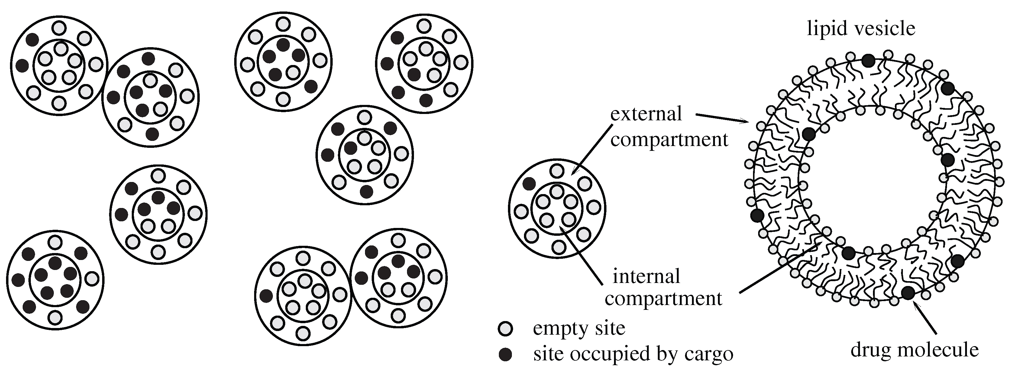
Figure 2.
Schematic representation of a carrier with , , , (middle). Inner and outer compartment are separated by the inner circle; empty sites are in gray and filled ones in black. Transfer of a cargo item from the external to the internal compartment results in , (left). Transfer of a cargo item from the internal to the external compartment results in , (right).
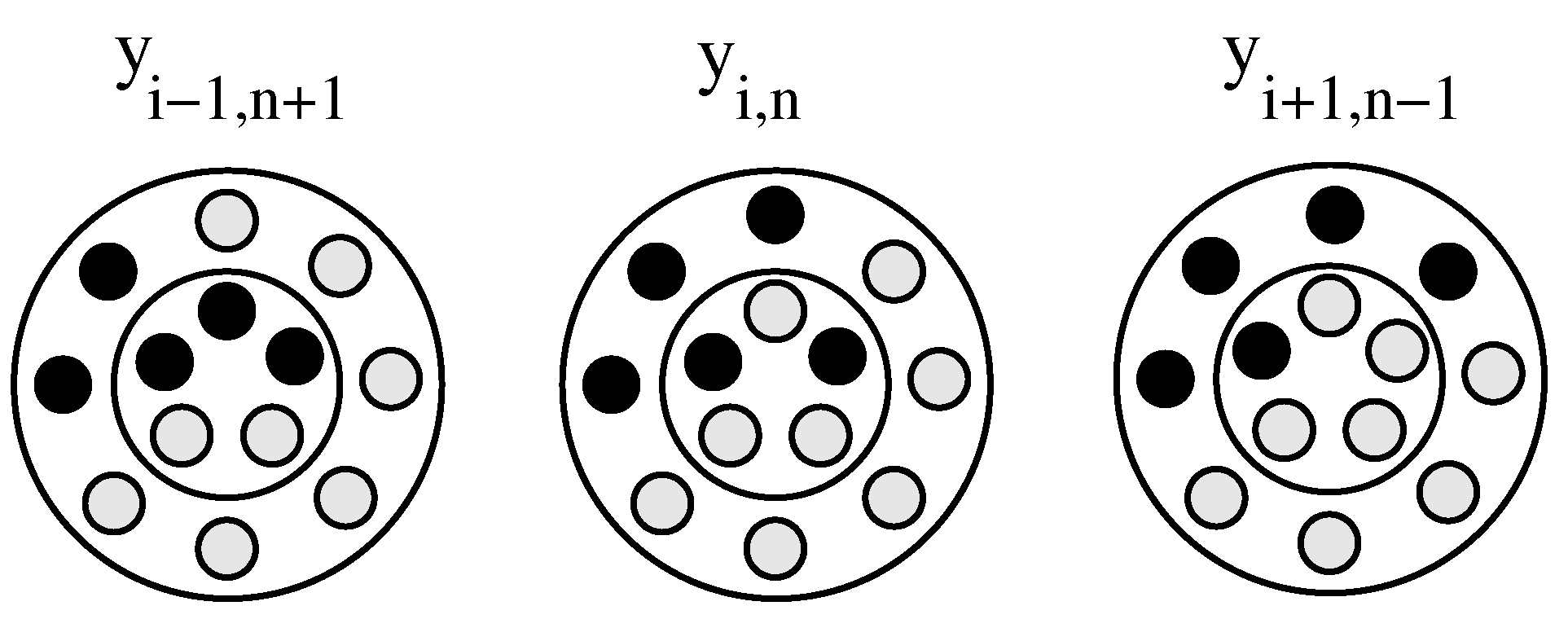
Figure 3.
Left diagram: The distribution according to Eq. 32 for as function of x and z for different times as indicated in the legend. Recall that Eq. 32 employs the specific choice and . For each time, is represented by four contour lines; is shown in purple (marked in the legend) and in red (marked “equilibrium” in the legend). The dashed line specifies the linear path along which the maximum of moves. Here, and according to Eq. 34. Right diagram: Cross sections of along the dashed line in left diagram, thus fixing . That is, is plotted for different times t, with the same color code as in the legend of the left diagram. The color-matching circles mark numerical solutions of the corresponding discrete rate equations specified in Eq. 3 with ; see the main text for all parameter specifications.
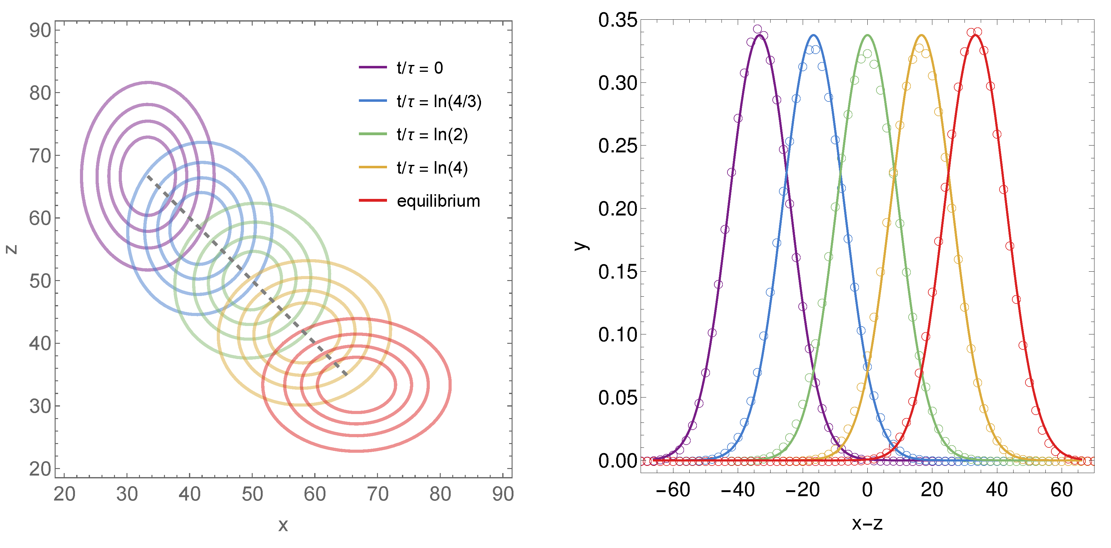
Figure 4.
The distribution for and with as function of x and z for different times as indicated in the legend. The initial distribution is the sum of two Gaussians according to Eq. 36 with . Our parameter choices for the left diagram, , , , and , represent a redistribution of the initial distribution in Figure 3 along lines of fixed , thus ensuring that the equilibrium distributions are the same. In contrast, the redistribution in the right diagram, enforced through our parameter choice , , , is along the x-axis, resulting in a different equilibrium distribution .
Disclaimer/Publisher’s Note: The statements, opinions and data contained in all publications are solely those of the individual author(s) and contributor(s) and not of MDPI and/or the editor(s). MDPI and/or the editor(s) disclaim responsibility for any injury to people or property resulting from any ideas, methods, instructions or products referred to in the content. |
© 2025 by the authors. Licensee MDPI, Basel, Switzerland. This article is an open access article distributed under the terms and conditions of the Creative Commons Attribution (CC BY) license (http://creativecommons.org/licenses/by/4.0/).
Copyright: This open access article is published under a Creative Commons CC BY 4.0 license, which permit the free download, distribution, and reuse, provided that the author and preprint are cited in any reuse.


